Spectra of Gauge Code Hamiltonians

Abstract

We study the spectral gap of frustrated spin (qubit) Hamiltonians constructed from quantum subsystem (gauge) codes. Such a Hamiltonian can be block diagonalized, with blocks labelled by eigenvalues of extensively many integrals of motion (stabilizers of the code.) Of particular interest is the 3D gauge color code, whose Hamiltonian has been conjectured to act as a quantum memory at finite temperature. Using Perron-Frobenius theory we constrain the location of first and second eigenvalues among the blocks of the Hamiltonian. This allows us to numerically find the gap of some large instances of the 3D gauge color code, which is compared to other frustrated spin Hamiltonians. Finally, we suggest a relation between bounded stabilizers and gapped spectra.

1 Introduction

In this paper we study the spectra of Hamiltonians built from spin one-half (qubit) Pauli operators. Sometimes these operators lead a double life, both as the energetic terms of a Hamiltonian model, and as the operators in a quantum error correcting code. In this case we have extensively many integrals of motion. These are the stabilizers of the code, and can be used to block diagonalize the Hamiltonion. This sets these models apart from other quantum condensed matter Hamiltonions, such as the Ising model, which has very few integrals of motion.

In Section 1.1 we show graphical depictions of some simple Hamiltonions and introduce the action of the Pauli $X$ and $Z$ operators. In Section 2 we study the group representation theory of subgroups of the (real) Pauli group on $n$ qubits. In Section 2.7 we find the irreducible representations of an arbitrary CSS gauge (subsystem) code.

In the computational basis, CSS gauge code Hamiltonians have positive off-diagonal entries and so can be viewed as the adjacency matrix of a weighted graph. This motivates the ideas in Section 3, where we use Perron-Frobenius theory to describe the low energy spectrum of such Hamiltonians. These are new results. Note that in this paper we use a “neg-Hamiltonian” convention, so that the groundspace corresponds to the highest eigenvalue.

In Section 4.4 we introduce the 3D gauge color code Hamiltonian[3, 4, 16]. We find that this model decomposes into six mutually commuting operators in Section 4.5. This gives an exponential reduction in the numerical difficulty of exactly diagonalizing this Hamiltonian, results of which we present in Section 5. These numerics show some evidence of a spectral gap, which is contrasted against models that are known to be gapless: the two and three dimensional compass model, the one dimensional $XY$-model and the one dimensional transverse field Ising model. The conjecture that the gauge color code model is gapped in turn lends weight to the possibility that this may be a self-correcting quantum memory [8]. Having a constant gap (bound from below) is also part of the story of topologically ordered phases [15, 8]. We also apply these techniques to a model we call the 2D $XY$-plaquette model, which has weight four gauge operators.

Finally in Section 6 we investigate the connection between the size of stabilizer generators and the gapped nature of the Hamiltonian. In particular, we suggest a relation between extensive stabilizer generators, and gapless excitations of the Hamiltonian. This is further application of the Perron-Frobenius theory in the context of Cheeger inequalities.

Acknowledgements.  The author would like to thank Andrew Doherty, Steven Flammia, Michael Kastoryano, Jiannis Pachos and Dan Browne.

1.1 Some motivating examples

Example 1.  We start our journey considering a two-dimensional state space. This space is blessed with two basis vectors $|{0}\rangle$ and $|{1}\rangle.$ The $Z$ and $X$ operators act on these states as:

From this picture we can see that $Z$ acts by stabilizing the state $|{0}\rangle$ and anti-stabilizing the $|{1}\rangle$ state. The $Z$ operator has been reduced to two operators each acting on a one dimensional subspace: $Z=+1\oplus-1.$ The $X$ operator serves to “bitflip” the state between these two subspaces.

But what happens if we get confused and end up swapping the $X$ and $Z$ operators? We would like to see the $X$ operator as stabilizing / anti-stabilizing two subspaces, together with the $Z$ operator as bitflipping between these. The trick is to consider the orbits of the operator we hope to act as a stabilizer. In this case there is only one orbit, $|{0}\rangle+|{1}\rangle$ and indeed, the $Z$ operator bitflips this to another state $|{0}\rangle-|{1}\rangle$ that is anti-stabilized by $X.$  

We are going to be considering Hamiltonians built from summing operators of this form. In this paper we use a “neg-Hamiltonian” convention, to save complicating expressions with negative signs. The ground space corresponds to the highest eigenvalue.

So building a Hamiltonian from a single $X$ or $Z$ term, we find the ground space as the stabilized space by summing over the orbit of that term. The other operator, which we call the adjacent operator, acts to bitflip between the eigenspaces.

Example 2.  To further elucidate this idea we turn to another example, which is a Hamiltonian built from three commuting and independent operators:

$$H=XXI+IXX+ZZZ.$$

Starting with $|{000}\rangle$ the terms of the Hamiltonian generate an orbit given by

$$\mathrm{Orbit}(|{000}\rangle)=\{|{000}\rangle,|{011}\rangle,|{110}\rangle,|{101}\rangle\}.$$

Notice that the $ZZZ$ term fixes all these states. Summing over this orbit we get the following ground state:

$$\mathrm{GS}=|{000}\rangle+|{011}\rangle+|{110}\rangle+|{101}\rangle.$$

We select three adjacent operators $ZII,IIZ,$ and $IXI,$ one for each of the stabilizer operators:

$$ZII:\mbox{GS} \mapsto|{000}\rangle+|{011}\rangle-|{110}\rangle-|{101}\rangle\ \mbox{anti-stabilized by}\ XXI,$$

$$IIZ:\mbox{GS} \mapsto|{000}\rangle-|{011}\rangle+|{110}\rangle-|{101}\rangle\ \mbox{anti-stabilized by}\ IXX,$$

$$IXI:\mbox{GS} \mapsto|{010}\rangle+|{001}\rangle+|{100}\rangle+|{111}\rangle\ \mbox{anti-stabilized by}\ ZZZ.$$

These adjacent operators form an abelian group of order $2^{3}=8$ and by applying each element of this group to the ground state we get a basis of our state space, which we call a symmetry invariant basis.

The adjacent operators are not unique in general. For this example we could have also chosen $IZZ,ZZI,XXX.$  

Example 3.  Now we consider a four qubit example:

$$H=XXII+IIXX+ZIZI+IZIZ.$$

This time the terms of the Hamiltonian do not generate an abelian group. We will call this group, as generated by the terms in the Hamiltonian, the gauge group, $G$. The stabilizer subgroup of $G$ will be the elements of $G$ that commute with every other element in $G.$ By inspection we see this group is generated by $S_{0}=\{XXXX,ZZZZ\}.$ We can extend these generators to a complete independent generating set for $G$ using the operators $R_{0}=\{XXII,ZIZI\}.$ These $R_{0}$ operators generate the reduced gauge group $R.$ The operators adjacent to $S_{0}$ we call the error operators $T_{0}$. We choose $T_{0}=\{ZZZI,IIIX\}.$ (Once again, these are not unique.) The logical operators are the $n$-qubit Pauli operators outside of the group $G$ that commute with $G.$ In this case they are generated by $L_{0}=\{XIXI,ZZII\}.$ All of this can be summarized in a table of adjacent pairs:

where the number of rows equals $n,$ each operator commutes with operators on other rows, and anticommutes with the operator on the same row. There is no need to include any phases ($\pm I$) in these tables because phases commute with everything. If we take all the entries in the left column we get the operators $\{ZZII,XXXX,ZZZZ,ZIZI\}.$ These generate an abelian group that stabilizes the state $|{\psi}\rangle=|{0000}\rangle+|{1111}\rangle.$ Let $r$ be the gauge operator $XXII$ adjacent to the stabilizer $ZIZI$, The state $|{\psi}\rangle$ then lies in the $G-$orbit

$$\{|{\psi}\rangle,r|{\psi}\rangle\}=\{|{0000}\rangle+|{1111}\rangle,|{1100}\rangle+|{0011}\rangle\}.$$

We use the $T_{0}$ operators $t_{1}=ZZZI$ and $t_{2}=IIIX$ to list three other $G-$orbits:

$$\{t_{1}|{\psi}\rangle,t_{1}r|{\psi}\rangle\},\{t_{2}|{\psi}\rangle,t_{2}r|{\psi}\rangle\},\{t_{1}t_{2}|{\psi}\rangle,t_{1}t_{2}r|{\psi}\rangle\}.$$

So now we have sixteen vectors, forming an orthogonal basis for the state space. This is the symmetry invariant basis for this Hamiltonian.

We can now arrange these basis vectors on the vertices of a four dimensional hypercube, such that each dimension corresponds to one of the adjacent $\tilde{X}_{i}$ bitflip operators. Such an arrangement has a cartesian product structure which induces a tensor product decomposition of the original state space that corresponds to the $\tilde{X}_{i}:$

The Hamiltonian acts on states by left multiplication. Because this action is a sum of gauge group elements, it will decompose into blocks, one for each $G-$orbit. We depict this action as a weighted graph, where we omit edges with zero weight:

Equivalently we use this basis to write the matrix for the Hamiltonian in block diagonal form:

$$H=\left(\begin{array}[]{cccc}2(X+Z)&0&0&0\\ 0&2X&0&0\\ 0&0&2Z&0\\ 0&0&0&0\\ \end{array}\right)\otimes I$$

This block diagonal form will be worked out for a general gauge group below and summarized in Section 2.5.  

So far we have been analysing the Hamiltonian in the symmetry invariant basis. The complete story of how this works is in Section 2 below. But we can also just fix the computational basis and examine the Hamiltonian in this basis. This leads to the Perron-Frobenius theory in Section 3.

2 Gauge code Hamiltonians

2.1 The Pauli group

The Pauli group $\mathcal{P}_{1}$ is normally defined as a set of matrices closed under matrix multiplication, but we can define it abstractly as the group generated by the (abstract) elements $\{\omega,X,Z\}$ with relations as follows:

$$\omega^{2}=I,\ X^{2}=I,\ Z^{2}=I,\ \omega X\omega X=I,\ \omega Z\omega Z=I,\ \mbox{and}\ \omega ZXZX=I,$$

where $I$ is the group identity. Actually, $\omega$ is generated by $X$ and $Z$, so it is not necessary to include $\omega$ in the generating set, but here it simplifies the relations. This group has eight elements, and is isomorphic to the dihedral group $D_{4}$, the symmetry group of a square.

To define the $n$-qubit Pauli group $\mathcal{P}_{n}$, we use the $2n+1$ element generating set

$$\{\omega,X_{1},..,X_{n},Z_{1},..,Z_{n}\}$$

with relation $\omega^{2}=I$ as before, and

$$\begin{array}[]{c}X_{i}^{2}=I,\ Z_{i}^{2}=I,\ \omega X_{i}\omega X_{i}=I,\ \omega Z_{i}\omega Z_{i}=I,\ \omega Z_{i}X_{i}Z_{i}X_{i}=I,\mbox{\ for\ }i=1,...n,\\ X_{i}X_{j}X_{i}X_{j}=I,\ Z_{i}Z_{j}Z_{i}Z_{j}=I,\ Z_{i}X_{j}Z_{i}X_{j}=I,\mbox{\ for\ }i,j=1,..,n,\ i\neq j.\end{array}$$ (1)

This abstract approach to the definition of a group is known as a group presentation. In general, this is a set of generators together with a set of relations satisfied by these generators.

Note that each of the generators squares to the identity, and of these, only $\omega$ commutes with every element of $\mathcal{P}_{n}.$ Therefore we will write $\omega$ as $-I,$ similarly $\pm I$ will denote the set $\{\omega,I\},$ and $-X$ is $\omega X$, etc.

We write the group commutator as $[[g,h]]:=ghg^{-1}h^{-1}$ and note the important commutation relation:

$$[[Z_{i},X_{j}]]=\left\{\begin{array}[]{ll}-I&\mbox{if}\ i=j,\\ I&\mbox{if}\ i\neq j.\end{array}\right.$$

If we take an arbitrary $g\in\mathcal{P}_{n}$ written as a product of the generators, it follows that we can rewrite this product uniquely as $g=\pm g_{1}...g_{n}$ where each $g_{i}$ is one of $I,Z_{i},X_{i}$ or $X_{i}Z_{i}$ for $i=1,..,n.$ Therefore, the size of the Pauli group is

$$|\mathcal{P}_{n}|=2^{2n+1}.$$

The subgroup of $\mathcal{P}_{n}$ generated by the elements $\{X_{1},...,X_{n}\}$ is denoted $\mathcal{P}_{n}^{X}.$ These are the $X$-type elements. Similarly, $\{Z_{1},...,Z_{n}\}$ generates the subgroup of $Z$-type elements $\mathcal{P}_{n}^{Z}$.

We now define the Pauli representation of the Pauli group as a group homomorphism:

$$\rho_{\mathrm{pauli}}:\mathcal{P}_{n}\to\mathrm{GL}(\mathbb{C}[2^{n}])$$

where $\mathbb{C}[2^{n}]$ is the $2^{n}$-dimensional state space of $n$ qubits. On the independent generators $\{X_{1},..,X_{n},Z_{1},..,Z_{n}\},\ \rho_{\mathrm{pauli}}$ is defined as the following tensor product of $2\times 2$ matrices:

$$\rho_{\mathrm{pauli}}(X_{i}):= \bigotimes_{j=1}^{n}\left\{\begin{array}[]{ll}\left(\begin{array}[]{ll}0&1\\ 1&0\end{array}\right)&\mbox{for $j=i$}\\ \\ \left(\begin{array}[]{ll}1&0\\ 0&1\end{array}\right)&\mbox{for $j\neq i$}\end{array}\right.$$

$$\rho_{\mathrm{pauli}}(Z_{i}):= \bigotimes_{j=1}^{n}\left\{\begin{array}[]{ll}\left(\begin{array}[]{ll}1&0\\ 0&-1\end{array}\right)&\mbox{for $j=i$}\\ \\ \left(\begin{array}[]{rr}1&0\\ 0&1\end{array}\right)&\mbox{for $j\neq i$}\end{array}\right.$$

2.2 Subgroups of the Pauli group

We now define an $n-$qubit gauge group to be any non-abelian subgroup $G$ of $\mathcal{P}_{n},$ defined by a set of generators $G_{0}\subset\mathcal{P}_{n},$

$$G:=\langle G_{0}\rangle.$$

Because $G$ is not abelian, it follows that $-I\in G.$ We also restrict $G_{0}$ to only contain Hermitian operators, which is equivalent to requiring that $g^{2}=I$ for all $g\in G_{0}.$

Now let $S$ be the largest subgroup of $G$ not containing $-I.$ $S$ is then an abelian subgroup, also known as the stabilizer subgroup. $G$ decomposes as a direct product:

$$G=S\times R,$$

where $R\cong\mathcal{P}_{r}$ for some $1\leq r\leq n,$ and $S\cong\mathbb{Z}_{2}^{m}$ for $0\leq m<n.$ Therefore,

$$|G|=|S||R|=2^{m+2r+1}.$$

We call $R$ the reduced gauge group. We consider both $S$ and $R$ to be subgroups of $G.$ Let $\phi:R\to\mathcal{P}_{r}$ be a group isomorphism, then $R_{0}:=\{\phi^{-1}(X_{i}),\phi^{-1}(Z_{i})\}_{i=1,..,r}$ is a set of independent generators of $R.$ We also let $S_{0}$ be a set of $m$ independent generators of $S.$

To find the cosets of $G$ in $\mathcal{P}_{n}$ we take the group closure of $\mathcal{P}_{n}-G$; when this is non-empty we only need to add $I$ and $-I.$ This is another gauge group, whose reduced gauge group is known as the logical operators $L$, and whose stabilizer subgroup is known as the error operators $T.$ Now any coset of $G$ can be written as $ltG$ with $l\in L$ and $t\in T.$ The size of $T$ equals the size of $S$: $|T|=|S|=2^{m}.$ If we let $L_{0}$ be an independent generating set for $L$ then we have the important formula:

$$n =\frac{1}{2}|L_{0}|+|S_{0}|+\frac{1}{2}|R_{0}|$$

$$=k+m+r$$

We summarize the information in this section in a table of Pauli group elements arranged in two columns and $n$ rows:

Here we show the $2n$ generators of $\mathcal{P}_{n}$ arranged so that each row contains a pair of generators, where each such generator anti-commutes with the operator on the same row and commutes with all the other operators in the table. Note that this is exactly the definition of the Pauli group via a presentation given in the previous section. Furthermore, the table shows $2k$ generators of $L$, $m$ generators each for $S$ and $T,$ and $2r$ generators of $R.$ The gauge group $G$ encloses $R$ and $S$, and one can immediately see how $L$ and $T$ also form a gauge group.

2.3 Representations of the Pauli group

We now define the Pauli representation of the Pauli group as a group homomorphism:

$$\rho_{\mathrm{pauli}}:\mathcal{P}_{n}\to\mathrm{GL}(\mathbb{C}[2^{n}])$$

where $\mathbb{C}[2^{n}]$ is the $2^{n}$-dimensional state space of $n$ qubits. On the independent generators $\{X_{1},..,X_{n},Z_{1},..,Z_{n}\},\ \rho_{\mathrm{pauli}}$ is defined as the following tensor product of $2\times 2$ matrices:

$$\rho_{\mathrm{pauli}}(X_{i}):= \bigotimes_{j=1}^{n}\left\{\begin{array}[]{ll}\left(\begin{array}[]{ll}0&1\\ 1&0\end{array}\right)&\mbox{for $j=i$}\\ \\ \left(\begin{array}[]{ll}1&0\\ 0&1\end{array}\right)&\mbox{for $j\neq i$}\end{array}\right.$$

$$\rho_{\mathrm{pauli}}(Z_{i}):= \bigotimes_{j=1}^{n}\left\{\begin{array}[]{ll}\left(\begin{array}[]{ll}1&0\\ 0&-1\end{array}\right)&\mbox{for $j=i$}\\ \\ \left(\begin{array}[]{rr}1&0\\ 0&1\end{array}\right)&\mbox{for $j\neq i$}\end{array}\right.$$

Normally the image of $\rho_{\mathrm{pauli}}$ is thought of as the Pauli group itself, and we are indeed free to think that way because $\rho_{\mathrm{pauli}}$ is a group isomorphism (onto its image).

Given a group representation $\rho:G\to GL(V)$ the character of $\rho$ is a function $\chi_{\rho}:G\to\mathbb{C}$ given by

$$\chi_{\rho}(g)=\mbox{Tr}\ \rho(g).$$

Given two functions $u,v:G\to\mathbb{C}$ we define the following inner product:

$$\langle u,v\rangle:=\frac{1}{|G|}\sum_{g\in G}u(g)\overline{v(g)}.$$

The character of the Pauli representation, $\chi_{{pauli}}:\mathcal{P}_{n}\to\mathbb{C}$ is given by:

$$\chi_{{pauli}}(g)=\sum_{v\in basis}\langle v|\rho_{{pauli}}(g)|v\rangle=\left\{\begin{array}[]{ll}\pm 2^{n}&\mbox{if}\ g=\pm I\\ 0&\mbox{otherwise}\end{array}\right.$$

Since $|\mathcal{P}_{n}|=2^{2n+1}$ it follows that $\langle\chi_{pauli},\chi_{pauli}\rangle=1$ and so $\rho_{pauli}$ is an irreducible representation of $\mathcal{P}_{n}.$

The only other irreps of $\mathcal{P}_{n}$ are the $1$-dimensional irreps $\rho:\mathcal{P}_{n}\to\mathbb{C}$ defined on the independent generators as:

$$\rho(X_{i})=\pm 1,\quad\rho(Z_{i})=\pm 1.$$

So we have $2^{2n}$ many $1$-dimensional irreps, and a single $2^{n}$-dimensional irrep. Summing the squares of the dimensions shows that we have a complete set of irreps of $\mathcal{P}_{n}.$

2.4 Representations of gauge groups

Although $\rho_{\mathrm{pauli}}$ restricted to a gauge group $G\subset\mathcal{P}_{n}$ serves as a representation of $G$ it is no longer irreducible. Our aim will be to decompose $\rho_{\mathrm{pauli}}$ into irreps of $G.$

The $1$-dimensional irreps $\rho:G\to\mathbb{C},$ are now defined by specifying the action of $\rho$ on the independent generators:

$$\rho(h)=\pm 1\ \mbox{for}\ h\in S_{0},\quad\rho(\phi^{-1}(X_{i}))=\pm 1,\quad\rho(\phi^{-1}(Z_{i}))=\pm 1.$$

This gives all $2^{m+2r}$ of the $1$-dimensional irreps.

The $2^{r}$-dimensional irreps are given by:

$$\rho(h)=\pm I^{\otimes r}\ \mbox{for}\ h\in S_{0},\quad\rho(\phi^{-1}(X_{i}))=X_{i},\quad\rho(\phi^{-1}(Z_{i}))=Z_{i}.$$

We are free to choose the signs of the $\rho(h)$ for each $h\in S_{0}.$ Hence there are $2^{m}$ many of these irreps. Each such choice corresponds to the choice of a syndrome vector $s(h)=\pm 1$, for $h\in S_{0},$ or alternatively, choice of an element $t\in T:$

$$\rho^{1}_{t}(h)=\left\{\begin{array}[]{ll}I^{\otimes r}&\mbox{if $th=ht$}\\ -I^{\otimes r}&\mbox{if $th=-ht$}\end{array}\right.$$

Because $G$ decomposes into a direct product $G=S\times\mathcal{P}_{r}$ we have the following representations:

$$\rho_{t}(g)=\rho^{1}_{t}(h)\rho^{r}_{pauli}(g^{\prime}),$$

where $g=hg^{\prime}$, $h\in S$, $g^{\prime}\in\mathcal{P}_{r}$ and $\rho^{r}_{pauli}$ is the $r$-qubit Pauli representation. The character for this representation is:

$$\chi_{t}(hg^{\prime})=\rho_{t}^{1}(h)\sum_{v\in basis}\langle v|\rho^{r}_{{pauli}}(g^{\prime})|v\rangle=\left\{\begin{array}[]{ll}\pm 2^{r}\rho_{t}^{1}(h)&\mbox{if}\ g^{\prime}=\pm I\\ 0&\mbox{otherwise}\end{array}\right.$$

We have that $|G|=2^{2r+m+1}$ and so $\langle\chi_{t},\chi_{t}\rangle=1$ and $\rho_{t}$ is an irreducible representation of $G.$ We now count the occurrences of this representation in $\rho^{r}_{pauli}$:

$$\langle\chi^{r}_{pauli},\chi_{t}\rangle =\frac{1}{|G|}\sum_{g\in G}\chi^{r}_{pauli}(g)\overline{\chi_{t}(g)}$$

$$=\frac{1}{2^{2r+m+1}}\sum_{g=\pm I}2^{n}2^{r}=\frac{2^{n+1+r}}{2^{2r+m+1}}=2^{k}$$

where $k$ is the number of logical qubits so that $n=r+m+k.$

In summary, the Pauli representation decomposes into $2^{m}$ many irreps $\rho_{t},$ each with dimension $2^{r},$ and appearing with multiplicity $2^{k}:$

$$\rho_{\mathrm{pauli}}=\bigoplus_{t\in T}\ \rho_{t}\otimes I^{\otimes k}$$

2.5 Block diagonalizing the Hamiltonian

The Hamiltonian of interest is an operator $H:\mathbb{C}[2^{n}]\to\mathbb{C}[2^{n}]$:

$$H:=\sum_{g\in G_{0}}\rho_{\mathrm{pauli}}(g).$$

Using the above decomposition we find:

$$H =\sum_{g\in G_{0}}\ \bigoplus_{l\in L,t\in T}\ \rho_{t}(g)$$

$$=\bigoplus_{l\in L,t\in T}\sum_{g\in G_{0}}\ \rho_{t}(g).$$

We will notate each block as $H_{t}:=\sum_{g\in G_{0}}\rho_{t}(g)$ for each irrep $\rho_{t}$ appearing in $H.$

The Hamiltonian is block diagonalized, with blocks indexed by operators $t$ in the abelian group $T$ and multiplicity $2^{k}:$

$$H=\bigoplus_{t\in T}\ H_{t}\otimes I^{\otimes k}.$$

More generally, we can assign real valued weights $J_{g}\in\mathbb{R}$ to each operator $g\in G_{0},$

$$H=\sum_{g\in G_{0}}J_{g}\rho_{\mathrm{pauli}}(g)=\bigoplus_{l\in L,t\in T}\sum_{g\in G_{0}}\ J_{g}\rho_{t}(g).$$

In other words, using weights does not change the block structure of $H.$

In the following sections we will forget the distinction between $g$ and $\rho_{\mathrm{pauli}}(g)$, so terms such as $Z$ and $X$ can be understood as the corresponding Pauli linear operators.

2.6 Symplectic decomposition of CSS gauge codes

In this section, and the remainder of this paper, we restrict our attention to gauge groups formed from terms in $\mathcal{P}_{n}^{X}\cup\mathcal{P}_{n}^{Z}.$ We call these CSS gauge codes. We next turn to a discussion of the symplectic structure of these operators.

Let $\mathcal{F}$ denote the finite field with two elements $0$ and $1$. Both $\mathcal{P}^{X}_{n}$ and $\mathcal{P}^{Z}_{n}$ are abelian groups, and can be identified with the additive group structure of the $n$ dimensional vector space over $\mathcal{F}:$

$$\mathcal{P}^{X}_{n}\cong\mathcal{F}^{n},\ \ \mathcal{P}^{Z}_{n}\cong\mathcal{F}^{n}.$$

We do this in the obvious way by sending $X_{i}$ to the basis vector with $1$ in the $i-$th entry, and similarly for each $Z_{i}$. We also identify the computational basis of our statespace $\mathbb{C}[2^{n}]$ with $\mathcal{F}^{n}$ in the obvious way:

$$\mathbb{C}[2^{n}]\cong\mathbb{C}[\mathcal{F}^{n}].$$

This has the potential to be very confusing, and so where appropriate we use $X$ and $Z$ subscripts.

$X$-type operators act on the $\mathbb{C}[\mathcal{F}^{n}]$ basis vectors using $\mathcal{F}$ addition:

$$g_{X}\in\mathcal{P}^{X}_{n}\cong\mathcal{F}^{n},\ \ g_{X}:v\longmapsto g_{X}+v$$

$Z$-type operators act on the $\mathbb{C}[\mathcal{F}^{n}]$ basis vectors using $\mathcal{F}$ inner product:

$$g_{Z}\in\mathcal{P}^{Z}_{n}\cong\mathcal{F}^{n},\ \ g_{Z}:v^{\top}\longmapsto g_{Z}v^{\top}$$

This is an $\mathcal{F}$ scalar, just zero or one. We think of this as a “syndrome”. This suggests that actually these $Z$-type operators live in the dual vector space $\mathcal{F}_{n}.$ Because of the underlying symmetry (and notational confusion) between the $X$ and $Z$-type operators, we make the convention that by default all our $\mathcal{F}$-vectors come as row vectors (ie. dual vectors). This means we use the transpose operator ^⊤ to indicate a primal (column) vector.

It doesn’t make sense to add an $X$-type operator and a $Z$-type operator:

$$g_{Z}+g_{X}\ \ \ \mbox{\emph{don't do this!!!}}$$

but it does make sense to take the inner product:

$$g_{Z}g_{X}^{\top}=g_{X}g_{Z}^{\top}.$$

This is an $\mathcal{F}$ scalar which gives the commutator of the two operators.

An $\mathcal{F}$-linear operator such as $A:\mathcal{F}^{n}\to\mathcal{F}^{m}$ acts on the left as $u^{\top}\mapsto Au^{\top}.$ It also acts on dual vectors as $A:\mathcal{F}_{m}\to\mathcal{F}_{n}$ which corresponds to acting on the right: $v\mapsto vA.$ We call the rowspace of $A$ the span and denote it as

$$\langle A\rangle=\{vA|v\in\mathcal{F}_{m}\}$$

The kernel of $A$ is defined as

$$\mathrm{ker}(A)=\{u^{\top}|u^{\top}\in\mathcal{F}^{n},\ \ Au^{\top}=0\}.$$

We wish to use this language to decompose a CSS gauge group $G.$ First we write the gauge group generators in terms of $X$-type and $Z$-type operators:

$$G_{0}=G_{X}\cup G_{Z}.$$

Following the theory from the previous section, we are going to rewrite the gauge group generators as a union of stabilizer generators $S_{0}=S_{X}\cup S_{Z}$ and reduced gauge generators $R_{0}=R_{X}\cup R_{Z}.$ Similarly, the error operators will be split into $X$-type and $Z$-type operators $T_{X}$ and $T_{Z}$ and finally the logical operators $L_{X}$ and $L_{Z}.$ We summarize all of these sets in the following table:

The solid rectangles indicate operators that span the $X$ and $Z$ parts of the gauge group, and the dashed rectangles indicate operators that do not live inside the gauge group.

We consider each of these blocks $L_{X},L_{Z},S_{X},T_{Z},T_{X},S_{Z},R_{X},R_{Z},$ as well as $G_{X},G_{Z},$ as either a set of $\mathcal{F}_{n}$ vectors (the rows) or as an $\mathcal{F}$-linear operator. For example, we write $u\in R_{X}$ to mean $u$ is a row of the matrix $R_{X}$.

Theorem (Decomposition).  Let $G$ be an $n$-qubit CSS gauge group with generators $G_{X}\cup~{}G_{Z}.$ We can construct a solution to the following $\mathcal{F}$-linear block matrix equation:

$$\left(\begin{array}[]{l}L_{X}\\ S_{X}\\ T_{X}\\ R_{X}\end{array}\right)\left(\begin{array}[]{l}L_{Z}\\ T_{Z}\\ S_{Z}\\ R_{Z}\end{array}\right)^{\top}=I,$$ (2)

such that $\langle S_{X}\rangle+\langle R_{X}\rangle=\langle G_{X}\rangle$ and $\langle S_{Z}\rangle+\langle R_{Z}\rangle=\langle G_{Z}\rangle,$ with $I$ the $n\times n$ identity matrix.

Proof: We first find the stabilizers $S_{Z}$. These are built out of $\mathcal{F}_{n}$ vectors from the span of $G_{Z}$ that commute with the rows of $G_{X}:$

$$\langle S_{Z}\rangle =\{\ vG_{Z}\ |\ vG_{Z}G_{X}^{\top}=0,\ \ v\in F_{|G_{Z}|}\ \}$$

$$=\{\ vG_{Z}\ |\ v^{\top}\in\mathrm{ker}(G_{X}G_{Z}^{\top})\ \}.$$

The generators (rows of $S_{Z}$) are then extracted from this span by row reduction. We swap the role of $X$ and $Z$ to find $S_{X}.$

We solve the block matrix equation (2), subject to the restriction that the rows of $R_{X}$ lie in the span of $G_{X}$, the rows of $L_{X}$ do not, and similarly for $R_{Z}$ and $L_{Z}.$ This set of 16 equations is quadratic in the unknown variables and so it is not obvious how to proceed, but it turns out a systematic way can be found.

We begin by finding $L_{Z}.$ These operators satisfy the following homology condition:

$$l_{Z}\in L_{Z}\ \ \mbox{is given by}\ \ l_{Z}^{\top}\in\mathrm{ker}(G_{X})\ \ \mbox{mod}\ \ \langle S_{Z}\rangle.$$

In other words, $L_{Z}$ is formed from a basis for the kernel of $G_{X}$ row-reduced using $S_{Z}.$ To be more specific we take any direct sum decomposition

$$\mathcal{F}_{n}=\langle S_{Z}\rangle\oplus V$$

then the operation of mod $\langle S_{Z}\rangle$ is the projection onto $V.$ We can explicitly write such a projector as the $n\times n$ matrix given by

$$P_{Z}=I+A^{\top}S_{Z}$$

where the matrix $A$ is the $m_{Z}\times n$ matrix consisting of the leading 1’s in any row-reduction of $S_{Z}.$ We define $P_{X}$ similarly for the operation of mod $\langle S_{X}\rangle.$

To find $L_{X}$ we solve the following $\mathcal{F}$-linear system:

$$\left(\begin{array}[]{l}L_{Z}\\ G_{Z}\\ \end{array}\right)L_{X}^{\top}=\left(\begin{array}[]{l}I\\ 0\end{array}\right)$$

The reduced gauge group matrix $R_{X}$ is found as a row-reduction of $G_{X}P_{X}.$ We cannot merely set $R_{Z}$ to be $G_{Z}P_{Z}$ because we also require $R_{X}R_{Z}^{\top}=I.$ Instead we define the auxiliary matrix $\widetilde{R}_{Z}$ to be a row-reduction of $G_{Z}P_{Z}.$

The error operators $T_{X}$ are then found as the solution to the $\mathcal{F}$-linear system:

$$\left(\begin{array}[]{l}L_{Z}\\ S_{Z}\\ \widetilde{R}_{Z}\end{array}\right)T_{X}^{\top}=\left(\begin{array}[]{l}0\\ I\\ 0\end{array}\right)$$

And then the operators $T_{Z}$ solve the $\mathcal{F}$-linear system:

$$\left(\begin{array}[]{l}L_{X}\\ S_{X}\\ T_{X}\\ R_{X}\end{array}\right)T_{Z}^{\top}=\left(\begin{array}[]{l}0\\ I\\ 0\\ 0\end{array}\right)$$

Finally at this point $R_{Z}$ is given as the solution to

$$\left(\begin{array}[]{l}L_{X}\\ S_{X}\\ T_{X}\\ R_{X}\end{array}\right)R_{Z}^{\top}=\left(\begin{array}[]{l}0\\ 0\\ 0\\ I\end{array}\right)$$

Note that $R_{Z}$ and $\widetilde{R}_{Z}$ have identical span and so we have $R_{Z}T_{X}^{\top}=0.$  

We call this array of eight $\mathcal{F}$-linear matrices an $(L,S,T,R)$-decomposition of the gauge group. In general this will not be unique for any given gauge group. Note that equation (2) is equivalent to the Pauli presentation (1).

2.7 CSS gauge code Hamiltonians

The complex Hilbert state space of our Hamiltonian has $2^{n}$ dimensions and we write this space as $\mathbb{C}[2^{n}]$. This notation is meant to suggest that we are forming a $\mathbb{C}$ vector space using $2^{n}$ “points” as basis vectors. Working in the computational basis, we do indeed have $2^{n}$ such points; these are the elements of $\mathcal{F}_{n}.$ And so we make the identification

$$\mathbb{C}[2^{n}]\cong\mathbb{C}[\mathcal{F}_{n}].$$

In other words, we are labeling our basis vectors with elements of $\mathcal{F}_{n}$ and therefore such notation as

$$\langle{u}|H|{v}\rangle$$

with $u,v\in\mathcal{F}_{n}$ makes sense. We will make further use of this below, by writing $\mathcal{F}$-vector space computations inside the Dirac brackets.

Returning to the code $(L,S,T,R)$-decomposition above, given the Pauli operator $t\in T$ such that $t=t_{X}t_{Z}$ (in $\mathcal{P}_{n}$) we get a basis for the irrep $\rho_{t}$:

$$\{|{vR_{X}+t_{X}}\rangle\ \mbox{such that}\ v\in\mathcal{F}_{r}\}.$$

In other words, the basis of the irrep $\rho_{t}$ is an affine subspace of $\mathcal{F}_{n}.$ Each such affine subspace is indexed by an element of $\mathcal{F}_{r}$ and all of these are translates of each other, so we make the following identification:

$$\mathbb{C}[\{vR_{X}+t_{X}\}_{v\in\mathcal{F}_{r}}]\cong\mathbb{C}[\mathcal{F}_{r}].$$

This will allow us to write the matrix entries of each block $H_{t}$ of the Hamiltonian as $\langle{u}|H_{t}|{v}\rangle$ for $u,v\in\mathcal{F}_{r}.$ We make this identification of affine subspaces not out of laziness but because it will help us to compare each of the Hamiltonian blocks $H_{t}$ below.

The computational basis identifies basis vectors of $\mathbb{C}[2^{n}]$ with elements of a finite vector space $\mathcal{F}_{n}$:

$$\mathbb{C}[2^{n}]\cong\mathbb{C}[\mathcal{F}_{n}].$$

The $(L,S,T,R)$-decomposition naturally decomposes $\mathcal{F}_{n}$ into $2^{m_{Z}+k}$ affine subspaces:

$$\{vR_{X}+t_{X}+l_{X}\}_{v\in\mathcal{F}_{r}}$$

for each $t_{X}\in\langle T_{X}\rangle,l_{X}\in\langle L_{X}\rangle.$ Each such affine subspace forms a symmetry invariant basis for the irreducible blocks $H_{t_{X},t_{Z}}$ of $H$, and can be naturally identified with $\mathcal{F}_{r}:$

$$H_{t_{X},t_{Z}}:\mathbb{C}[\mathcal{F}_{r}]\to\mathbb{C}[\mathcal{F}_{r}].$$

We now wish to understand the action of the gauge group on each of its irreps. Starting with the $t_{X},t_{Z}=0,0$ irrep, each stabilizer has a trivial action. In $\mathcal{F}^{n}$ this corresponds to the additive action of the zero vector.

States $u\in\langle R_{X}\rangle$ can be built from a vector matrix product

$$u=vR_{X}$$

with $v\in\mathcal{F}_{r}.$ Since $R_{X}R_{Z}^{\top}=I$ we can write $v=uR_{Z}^{\top}.$ Each $g_{X}\in G_{X}$ acts on $u$ to give

$$u_{1} =(u+g_{X})\ \mbox{mod}\ \langle S_{X}\rangle$$

$$=(u+g_{X})P_{X}$$

$$=(vR_{X}+g_{X})P_{X}.$$

writing $u_{1}=v_{1}R_{X}$ we then have

$$v_{1} =(vR_{X}+g_{X})P_{X}R_{Z}^{\top}$$

$$=v+g_{X}R_{Z}^{\top}.$$

So we have that working in the computational basis, the action of the $X$ part of the gauge group in the $t_{X},t_{Z}=0,0$ irrep is to send $v\in\mathcal{F}_{r}$ to $v+g_{X}R_{Z}^{\top}.$ In summary, we have the following contributions from the $G_{X}$ terms of the Hamiltonian:

$$\bigl{\langle}\,{v}\,\bigr{|}H_{0,0}\bigl{|}\,{v+g_{X}R_{Z}^{\top}}\,\bigr{\rangle}\mathrel{+}=1,\ \ \mbox{for}\ g_{X}\in G_{X},v\in\mathcal{F}_{r}$$

where we use the $\mathrel{+}=$ notation because there may be other contributions to the same entry. These terms will always be off the diagonal unless $g_{X}$ is a stabilizer.

The action of the $G_{Z}$ gauge group contributes to the diagonal of $H.$ These diagonal terms apply a kind of “potential energy” penalty to the basis states that depends on the syndrome vector:

$$\mbox{syndrome}(u)=G_{Z}u^{\top}$$

for $u^{\top}\in\mathcal{F}^{n}.$ This is an $\mathcal{F}$-vector that has one entry for each row of $G_{Z}.$ Writing $|G_{Z}|$ for the number of these rows, and using a weight function $w$ that just counts the number of non-zero entries in any $\mathcal{F}$-vector we have the following contributions to the Hamiltonian:

$$\bigl{\langle}\,{v}\,\bigr{|}H_{0,0}\bigl{|}\,{v}\,\bigr{\rangle}\mathrel{+}=|G_{Z}|-2w(G_{Z}R_{X}^{\top}v^{\top}),$$

for $v\in\mathcal{F}_{r}.$

Adding up all of the above we have in summary,

$$H_{0,0}=\sum_{\begin{subarray}{c}v\in\mathcal{F}_{r}\\ g_{X}\in G_{X}\end{subarray}}\bigl{|}\,{v+g_{X}R_{Z}^{\top}}\,\bigr{\rangle}\bigl{\langle}\,{v}\,\bigr{|}+\sum_{v\in\mathcal{F}_{r}}\bigl{(}|G_{Z}|-2w(G_{Z}R_{X}^{\top}v^{\top})\bigr{)}\ \bigl{|}\,{v}\,\bigr{\rangle}\bigl{\langle}\,{v}\,\bigr{|}.$$ (3)

For any $t_{X}\in\langle T_{X}\rangle$ the Hamiltonian block $H_{t_{X},0}$ has entries indexed by basis vectors:

$$u=vR_{X}+t_{X}$$

this means that the $G_{X}$ gauge terms have the same effect on $H_{t_{X},0}$ as $H_{0,0}$ and only the diagonal has changed:

$$H_{t_{X},0}=\sum_{\begin{subarray}{c}v\in\mathcal{F}_{r}\\ g_{X}\in G_{X}\end{subarray}}\bigl{|}\,{v+g_{X}R_{Z}^{\top}}\,\bigr{\rangle}\bigl{\langle}\,{v}\,\bigr{|}+\sum_{v\in\mathcal{F}_{r}}\bigl{(}|G_{Z}|-2w(G_{Z}R_{X}^{\top}v^{\top}+G_{Z}t_{X}^{\top})\bigr{)}\ \bigl{|}\,{v}\,\bigr{\rangle}\bigl{\langle}\,{v}\,\bigr{|}$$ (4)

The general form of each Hamiltonian block is:

$$H_{t_{X},t_{Z}}=\sum_{\begin{subarray}{c}v\in\mathcal{F}_{r}\\ g_{X}\in G_{X}\end{subarray}}\eta(t_{Z}g_{X}^{\top})\ \bigl{|}\,{v+g_{X}R_{Z}^{\top}}\,\bigr{\rangle}\bigl{\langle}\,{v}\,\bigr{|}+\sum_{v\in\mathcal{F}_{r}}\bigl{(}|G_{Z}|-2w(G_{Z}R_{X}^{\top}v^{\top}+G_{Z}t_{X}^{\top})\bigr{)}\ \bigl{|}\,{v}\,\bigr{\rangle}\bigl{\langle}\,{v}\,\bigr{|}$$ (5)

Here we use $\eta$ to send $t_{Z}g_{X}^{\top}$ which is an $\mathcal{F}$ value to the multiplicative subgroup $\{\pm 1\}$ of $\mathbb{C}:$

$$\eta(0)=1,\ \eta(1)=-1.$$

The $\eta(t_{Z}g_{X}^{\top})$ term is a kind of parity check that picks up one phase flip for (some of) the $X$-type stabilizers found in $g_{X}.$ This works because $T_{Z}$ is a left inverse of $S_{X}^{\top}.$ The $t_{Z}\in\langle T_{Z}\rangle$ selects which $X$-type stabilizers act as $-1$ in this irrep.

In summary, we have the complete representation theory for $CSS$ gauge code Hamiltonians.

3 Perron-Frobenius theory

In this section we present applications of Perron-Frobenius theory to finding bounds on the spectrum of CSS gauge code Hamiltonians. These are new results.

A non-negative matrix is a real matrix $\Gamma$ with entries $\Gamma_{ij}\geq 0.$ A positive vector $|{v}\rangle$ is a real vector with all-positive entries. Similarly, a non-negative vector has all entries real and non-negative.

Given a non-negative matrix $\Gamma:\mathbb{C}[V]\to\mathbb{C}[V]$ we will also view this as a weighted graph on a set of vertices $V.$ This associates a directed edge $i\mapsto j$ for every positive entry $\Gamma_{ij}>0.$

A non-negative matrix $\Gamma:\mathbb{C}[V]\to\mathbb{C}[V]$ is called irreducible if the following holds: for any pair $u,v\in V$ with $u\neq v$ there is a sequence $\{u_{i}\}_{i=1,...,n}$ such that $u_{1}=u$ and $u_{n}=v$ and

$$\langle{u_{i+1}}|\Gamma|{u_{i}}\rangle>0\ \ \ \mbox{for}\ \ i=1,...,n-1.$$

This says that viewed as a weighted graph, $\Gamma$ is “connected”. That is, we can find a directed path in $\Gamma$ from any vertex $u$ to any other vertex $v$. In general, this is a coarser notion than the (vector space) reducibility used in the representation theory above. The reason why is that when reducing a matrix we work with a fixed basis.

The following theorem originally appeared in the work of Frobenius [13], who was building on previous results of Perron [18]. See also the recent book [2].

Theorem (Perron-Frobenius).  Let $\Gamma$ be a non-negative irreducible matrix. Then $\Gamma$ has a positive real eigenvalue $\lambda$ equal to its spectral radius, this eigenvalue is non-degenerate and can be associated with a positive eigenvector $|{v}\rangle$. Furthermore, any other non-negative eigenvector of $\Gamma$ is a scalar multiple of $|{v}\rangle.$  

Therefore, when $\Gamma$ is a symmetric non-negative irreducible matrix, we see that this theorem implies that the top eigenvalue of $\Gamma$ is non-degenerate and associated with a positive eigenvalue.

Given a matrix $\Gamma$ with $\Gamma_{ij}\geq 0,i\neq j$ we can find a spectral shift operator which is a constant multiple of the identity $+cI$, such that $\Gamma+cI$ is a non-negative matrix. We refer to such a matrix $\Gamma$ as stoquastic [7, 6]. When $\Gamma$ is also irreducible we can therefore apply the Perron-Frobenius theorem with the proviso that the eigenvalues are shifted by some constant.

For a linear operator $A$ we will use notation $\lambda_{1}(A)$, $\lambda_{2}(A),$ etc., to denote the (real) eigenvalues of $A$, ordered as:

$$\lambda_{1}(A)\geq\lambda_{2}(A)\geq...$$

Similarly, the notation $v_{1}(A),v_{2}(A),$ etc., refers to the associated eigenvectors.

Given a CSS gauge code Hamiltonian $H,$ let the matrix for $H$ in the computational basis be $\Gamma.$ We see that the diagonal entries of $\Gamma$ come from the $Z$-type operators and the off-diagonal entries come from $X$-type operators. Therefore, the off-diagonal entries of $\Gamma$ are non-negative and so this matrix is stoquastic. In the language of graph theory, $\Gamma$ has vertices the $2^{n}$ computational basis elements, and edges:

$$|{v}\rangle\mapsto g_{X}|{v}\rangle,\ \ \mbox{for all}\ \ v\in\mathcal{F}_{n},g_{X}\in G_{X}.$$

These are undirected edges because $g_{X}^{2}=I.$ We also add weighted loops corresponding to the $Z$-type gauge operators:

$$|{v}\rangle\mapsto\sum_{g_{Z}\in G_{Z}}g_{Z}|{v}\rangle,\ \ \mbox{for all}\ \ v\in\mathcal{F}_{n}.$$

We can think of the $Z$-type operators as potential energy, and the $X$-type operators as kinetic energy. This is consistent with the classical use of the (real) symplectic group, where dynamical variables come in position and momentum pairs.

Lemma 4.  Given a CSS gauge code Hamiltonian $H$, writing the matrix for $H$ in the computational basis as $\Gamma,$ this matrix decomposes into irreducible stoquastic matrices $\Gamma_{t_{X}}$ indexed by $t_{X}\in\langle T_{X}\rangle$ with multiplicity $2^{k}$:

$$\Gamma=\bigoplus_{\begin{subarray}{c}t_{X}\in\langle T_{X}\rangle\\ l_{X}\in\langle L_{X}\rangle\end{subarray}}\Gamma_{t_{X}}.$$

Proof: Once again, we identify the computational basis with the elements of $\mathcal{F}_{n}.$ As a graph, $\Gamma$ has vertices $|{v}\rangle$ for $v\in\mathcal{F}_{n}$, and edges $|{v}\rangle\mapsto g|{v}\rangle$ for $v\in\mathcal{F}_{n},g\in G_{X}.$ This means that paths starting from $|{v}\rangle$ are given by words $g_{i}...g_{1}$ built from the elements of the group $G_{X}:$

$$|{v}\rangle\mapsto g_{1}|{v}\rangle\mapsto...\mapsto g_{i}...g_{1}|{v}\rangle.$$

Switching to the additive $\mathcal{F}_{n}$ notation, we therefore have that vertices $|{v}\rangle$ and $|{u}\rangle$ are in the same component of $\Gamma$ iff $|{u}\rangle=|{v+g_{X}}\rangle$ for some $g_{X}\in\langle G_{X}\rangle.$ The vertices

$$\Bigl{\{}\bigl{|}\,{t_{X}+l_{X}}\,\bigr{\rangle}\Bigr{\}}_{t_{X}\in\langle T_{X}\rangle,\ l_{X}\in\langle L_{X}\rangle}$$

each live in one component of $\Gamma$, and each component of $\Gamma$ contains one of these vertices. This shows that these components are in bijective correspondence with pairs $(t_{X},l_{X})$ where $t_{X}\in\langle T_{X}\rangle,\ l_{X}\in\langle L_{X}\rangle$. We write each such component as $\Gamma_{t_{X},l_{X}}$. The vertices contained in the $\Gamma_{t_{X},l_{X}}$ component are given by a coset of $G_{X}$ in $\mathcal{F}_{n}:$

$$\Bigl{\{}\bigl{|}\,{vS_{X}+uR_{X}+t_{X}+l_{X}}\,\bigr{\rangle}\Bigr{\}}_{v\in\mathcal{F}_{m_{X}},u\in\mathcal{F}_{r}}.$$

When comparing these different components of $\Gamma$, we will identify these cosets, and so consider $\Gamma_{t_{X},l_{X}}$ as an operator:

$$\Gamma_{t_{X},l_{X}}:\mathbb{C}[\mathcal{F}_{m_{X}}\oplus\mathcal{F}_{r}]\to\mathbb{C}[\mathcal{F}_{m_{X}}\oplus\mathcal{F}_{r}].$$

Because each of these components is independant of $l_{X}$ we write it as $\Gamma_{t_{X}}.$  

Lemma 5.  Given a CSS gauge code Hamiltonian $H$, and matrix $\Gamma$ in the computational basis with irreducible components $\Gamma_{t_{X}}$, with $t_{X}\in\langle T_{X}\rangle$, the first eigenvalue of each $\Gamma_{t_{X}}$ is non-degenerate and is associated with an eigenvector with positive entries.

Proof: We already established that $\Gamma$ and therefore $\Gamma_{t_{X}}$ is stoquastic. By the previous lemma $\Gamma_{t_{X}}$ is irreducible. We apply the Perron-Frobenius theorem and the result follows.  

Any stabilizer that acts as $-1$ in a given block of the Hamiltonian we will call a frustrated stabilizer (with respect to the given block.) Similarly, a satisfied stabilizer acts as $+1$ in a given block of the Hamiltonian. We will call a vector stabilized if it is a $+1$ eigenvector of every stabilizer in the given gauge group.

Lemma 6.  Given a CSS gauge code Hamiltonian $H$, every groundstate of $H$ is stabilized.

Proof: The set of top eigenvectors

$$\bigl{\{}v_{1}(\Gamma_{t_{X}})\bigr{\}}_{t_{X}\in\langle T_{X}\rangle}$$

must contain a basis for the groundspace of $H.$ Let such a basis vector be $|{v}\rangle=v_{1}(\Gamma_{t_{X}})$ for some $t_{X}.$ This vector is positive by Lemma 3. Any stabilizer commutes with every element of the gauge group and so must have $|{v}\rangle$ as an eigenvector. Because any $X$-type operator acts by permuting the computational basis elements and $|{v}\rangle$ is positive it must be stabilized by the $X$-type stabilizers. Therefore, we can find a basis for the groundspace of $H$ consisting of vectors that are fixed by $X$-type stabilizers.

We repeat this argument for $H$ switching to the $|{\pm}\rangle$ basis. This will give a basis for the groundspace consisting of vectors that are fixed by the $Z$-type stabilizers. Therefore the entire groundspace must be stabilized.  

Proposition 7.  For any CSS gauge code Hamiltonian $H$ we have:

$$\lambda_{1}(H)=\lambda_{1}(H_{0,0})$$

and for $t_{X}\in\langle T_{X}\rangle,t_{Z}\in\langle T_{Z}\rangle$ with $t_{X}\neq 0$ or $t_{Z}\neq 0$,

$$\lambda_{1}(H)>\lambda_{1}(H_{t_{X},t_{Z}}).$$

Proof: The vectors in the space that $H_{t_{X},t_{Z}}$ operates on are stabilized iff $t_{X}=0$ and $t_{Z}=0$, and so the result follows as a consequence of the previous lemma.  

The following lemma is used in section 2.8 below.

Lemma 8.  Given a CSS gauge code Hamiltonian $H$ and $t_{X}\in\langle T_{X}\rangle,$ the matrices for $H_{t_{X},0}$ in the symmetry invariant basis are irreducible stoquastic.

Proof: From equation (4) we see that the nonzero, nondiagonal entries of the matrices $H_{t_{X},0}$ are $+1,$ and so this matrix is stoquastic. This matrix is irreducible because as an operator it is irreducible.  

So far, the Perron-Frobenius theory has been fruitful, telling us that the first eigenvalue of $H$ resides in the spectrum of the block $H_{0,0}$. The next goal is to search for the second eigenvalue of $H$.

Lemma 9.  Let $H$ be a CSS gauge code Hamiltonian, with matrix $\Gamma$ in the computational basis and irreducible components $\Gamma_{t_{X}}$. We have

$$\Gamma_{t_{X}}=\bigoplus_{t_{Z}\in\langle T_{Z}\rangle}H_{t_{X},t_{Z}}.$$

Proof: Irreducibility of matrices is a coarser property than irreducibility of representations. The result follows by considering eigenspaces of stabilizers.  

Proposition 10.  For a gauge code Hamiltonian $H$,

$$\lambda_{1}(H_{t_{X},0}) >\lambda_{1}(H_{t_{X},t_{Z}})\ \ \ \mbox{and}\ \$$

$$\lambda_{1}(H_{0,t_{Z}}) >\lambda_{1}(H_{t_{X},t_{Z}}),$$

where $t_{X}\neq 0$ and $t_{Z}\neq 0.$

Proof: Let $H$ be a CSS gauge code Hamiltonian. Let $\Gamma$ be the matrix for $H$ in the computational basis, with $\Gamma_{t_{X}}$ the irreducible matrix components. From Lemma 3,

$$\Gamma_{t_{X}}=\bigoplus_{t_{Z}\in\langle T_{Z}\rangle}H_{t_{X},t_{Z}}.$$

And, by Lemma 3 the first eigenvector of $\Gamma_{t_{X}}$ is non-degerate and positive. This will be an eigenvector of each stabilizer, and in particular must be fixed by the $X$-type stabilizers. Therefore, this eigenvalue is in the spectrum of $H_{t_{X},0}$ and no other $H_{t_{X},t_{Z}}$ with $t_{Z}\neq 0.$ This shows $\lambda_{1}(H_{t_{X},0})>\lambda_{1}(H_{t_{X},t_{Z}}).$ We switch to the $|{\pm}\rangle$ basis and repeat this argument to obtain the second inequality.  

To find the spectral gap of a weakly self-dual gauge code Hamiltonian $H$, we need only examine the top two eigenvalues of $H_{0,0}$ and the top eigenvalue of $H_{t_{X},0}$ for each $t_{X}\in T_{X}.$ We summarize this in the theorem:

Theorem 11.  For a weakly self-dual gauge code Hamiltonian $H$, the spectral gap is given by:

$$\min\bigl{\{}\lambda_{1}(H_{0,0})-\lambda_{2}(H_{0,0}),\min_{t_{X}\in\langle T_{X}\rangle}\{\lambda_{1}(H_{0,0})-\lambda_{2}(H_{t_{X},0})\}\bigr{\}}$$

Proof: Combine Proposition 3 with Proposition 3. By weak self-duality, the spectrum of $H_{t_{X},t_{Z}}$ equals the spectrum of $H_{t^{\prime}_{X},t^{\prime}_{Z}}$ for some $t^{\prime}_{X}\in\langle T_{X}\rangle,t^{\prime}_{Z}\in\langle T_{Z}\rangle.$  

4 Models

A CSS gauge code is self-dual when the $X$-type and $Z$-type gauge generators are equal:

$$G_{X}=G_{Z}.$$

A CSS gauge code is weakly self-dual when there is a permutation $P$ on the set of $n$ qubits that induces equality of the gauge generators:

$$G_{X}P=G_{Z},$$

where we write $P$ as an $n\times n$ permutation matrix.

4.1 Transverse field Ising model

For the one dimensional transverse field Ising model, we have

$$G_{0}=\{X_{i},Z_{i}Z_{i+1}\ \ \mbox{for}\ \ i=1,...,n\},$$

with periodic boundary conditions. This model has one extensive $X$-type stabilizer and no logical operators. This model is also exactly solvable, with gap going to zero as the system size grows [19].

4.2 $XY$-model

The $XY$-model [19] lives on a one dimensional chain of $n$ qubits. We write the gauge group generators as

$$G_{0}=\{X_{i}X_{i+1},Z_{i}Z_{i+1}\ \ \mbox{for}\ \ i=1,...,n\}$$

with periodic boundary conditions. This is a self-dual CSS gauge code. We focus on the $n$ even $XY$-model, which is exactly solvable, with gap going to zero as the system size grows [17]. This model has no logical operators, one $X$-type stabilizer and one $Z$-type stabilizer, both extensive. Normally the gauge operators are written as $\{X_{i}X_{i+1},Y_{i}Y_{i+1}\ \mbox{for}\ i=1,...,n\}$ but note that there is an automorphism of the Pauli group that sends $G_{0}$ to these operators.

We also consider a two dimensional version of this model, which we call the 2D $XY$-plaquette model. Qubits live on a 2D periodic lattice of $l\times l$ sites. This is also a self-dual CSS gauge code, with gauge group generators

$$G_{0}=\{X_{ij}X_{i+1,j}X_{i,j+1}X_{i+1,j+1},\ Z_{ij}Z_{i+1,j}Z_{i,j+1}Z_{i+1,j+1}\ \ \mbox{for}\ \ i,j=1,...,l\}.$$

For $l$ even, we have $2l-3$ extensive stabilizer generators of $X$ type:

$$\prod_{i=1}^{l}X_{ij}X_{i,j+1}\ \ \mbox{for}\ \ j=1,...,l-1,\ \ \prod_{j=1}^{l}X_{ij}X_{i+1,j}\ \ \mbox{for}\ \ j=1,...,l-2,$$

and similarly for the $Z$-type stabilizer generators. This model has two logical qubits with logical operators generated by

$$L_{0}=\Big{\{}\prod_{i=1}^{l}X_{i1},\ \prod_{i=1}^{l}Z_{i1},\ \prod_{j=1}^{l}X_{1j},\ \prod_{j=1}^{l}Z_{1j}\Big{\}}.$$

4.3 Compass model

Here we consider the compass model [1]. For the 2D model, qubits live on a periodic square lattice of $l\times l$ sites. The generators of the gauge group are

$$G_{0}=\big{\{}X_{ij}X_{i,j+1},\ Z_{ij}Z_{i+1,j}\ \ \mbox{for}\ \ i,j=1,...,l\big{\}}.$$

The generators for the stabilizers are extensive and given by

$$S_{0}=\Big{\{}\prod_{i=1}^{l}X_{ij}X_{i,j+1},\ \prod_{i=1}^{l}Z_{ji}Z_{j+1,i}\ \ \mbox{for}\ \ j=1,...,l-1\Big{\}}.$$

The logical operators are generated by $L_{0}=\big{\{}\prod_{i}X_{i1},\prod_{j}Z_{1j}\big{\}}.$ This model is weakly self-dual when we transpose the square lattice of $l\times l$ qubits.

The 3D compass model has qubits on a periodic lattice of $l\times l\times l$ sites. The generators of the gauge group and stabilizer group are

$$G_{0} =\big{\{}X_{ijk}X_{i+1,j,k},\ X_{ijk}X_{i,j+1,k},\ Z_{ijk}Z_{i,j+1,k},\ Z_{ijk}Z_{i,j,k+1}\ \ \mbox{for}\ \ i,j,k=1,...,l\big{\}}$$

$$S_{0} =\Big{\{}\prod_{j,k=1}^{l}X_{ijk}X_{i+1,j,k},\ \prod_{j,k=1}^{l}Z_{jki}Z_{j,k,i+1}\ \ \mbox{for}\ \ i=1,...,l-1\Big{\}}.$$

The 3D compass model is also weakly self-dual, and has extensive stabilizer generators.

4.4 Gauge color code model

The three dimensional gauge color code [3, 4, 16] is a self-dual CSS gauge code. It is based on the following geometric construction known as a colex [5]. We begin with a tetrahedron and subdivide it into finitely many convex 3-dimensional polytopes, or bodies. Each body has a boundary consisting of 0-dimensional cells which we call vertices, 1-dimensional cells called edges and 2-dimensional cells called faces. By a cell we mean any of these 0,1,2 or 3-dimensional convex polytopes. Any two bodies in this tetrahedral subdivision will have either empty intersection or otherwise intersect on a common vertex, edge or face. When the intersection is on a face these two bodies are called adjacent. Two vertices in the same edge will also be called adjacent. Each body is colored by one of four colors, either taken to be red, green, blue, yellow or otherwise an element of the set $\{1,2,3,4\}.$ The four exterior triangular faces of the bounding tetrahedron are called regions, and the intersection of three regions is called a corner. A cell not contained within any region is called an interior cell.

This colored cellulation is required to have the following further properties:

1. Adjacent bodies have different colors.

2. Each region has a unique color such that no bodies intersecting that region has that color.

3. All vertices are adjacent to four other vertices, except for the corner vertices which are adjacent to three other vertices.

Here we show some instances of this construction, along with the colors of the unobscured bodies. Each instance is labeled by the number of vertices $n$.

We note the following consequences of the above conditions. Every face supports an even number of vertices. Thinking of each region as corresponding to a missing body, each edge is then contained in the boundary of three bodies. This means we can associate a unique color to each edge, which is also the color of two bodies intersecting a vertex of the edge. That is, each edge joins two bodies of the same color. Each face bounds two bodies, and so we color each face with the two colors of these bodies.

Using this cellulation we now construct the gauge code. Qubits are associated with the $n$ vertices. We associate operators to other cells, or union of cells, by using the contained vertices as support. Because this is a self-dual code, the same definitions apply for both the $X$-type and $Z$-type operators. The $X/Z-$type gauge group is generated by $X/Z-$type operators supported on each face. The $X/Z-$type stabilizer group is generated by $X/Z-$type operators supported on each body. Therefore, the stabilizer generators are non-extensive (have bounded size). There is one $X/Z-$type logical operator generator and these are given by $X/Z-$type operators supported on any region.

4.5 Commuting ideals of gauge codes

When the gauge group generators $G_{0}$ can be partitioned into mutually commuting parts, the corresponding Hamiltonian can be written as a sum of mutually commuting operators. For example, for $n$ even, the $XY$-model gauge generators can be partitioned into two mutually commuting parts:

$$G_{0}= \{X_{i}X_{i+1},Z_{i}Z_{i+1}\ \ \ \mbox{for}\ \ i=1,...,n.\}$$

$$= \{X_{i}X_{i+1},Z_{i+1}Z_{i+2}\ \ \ \mbox{for}\ \ i=1,3,..,n-1.\}$$

$$\cup\{X_{i}X_{i+1},Z_{i+1}Z_{i+2}\ \ \ \mbox{for}\ \ i=2,4,..,n.\}.$$

In general we call these parts commuting ideals. Let $a\in A$ index these parts. For a partition of the gauge group into mutually commuting parts $G_{0}^{a}$, we write the Hamiltonian $H$ as a sum of mutually commuting operators $H^{a}=\sum_{g\in G_{0}^{a}}g:$

$$G_{0}=\bigcup_{a\in A}G_{0}^{a},\ \ H^{a}=\sum_{g\in G_{0}^{a}}g,\ \ H=\sum_{a\in A}H^{a}.$$

Applying the Decomposition Theorem to each of the $H^{a}$ we obtain the matrices $L^{a},S^{a},T^{a},R^{a}$ with $X,Z$ subscripts. It follows that each Hamiltonian block $H_{t_{X},t_{Z}}$ can be written as a sum of mutually commuting operators:

$$H_{t_{X},t_{Z}}=\sum_{a}H^{a}_{t_{X}S_{Z}^{a\top}T_{X}^{a},t_{Z}S_{X}^{a\top}T_{Z}^{a}}.$$

We next examine the commuting ideal structure of the 3D gauge color code. Two face operators, of $X$-type and $Z$-type, will anti-commute precisely when they intersect on a single vertex. And this only happens when such faces have disjoint coloring. Here we show an example of this in the $n=39$ model:

There are three of these arrangements, each corresponding to the three ways of partitioning the set of colors into two sets of two. It follows that $G_{0}$ can be partitioned into six commuting ideals.

In a similar vein, for the 2D $XY$-plaquette model (with $l$ even) we find that the gauge group partitions into four commuting ideals. Each ideal corresponds to a choice of a checkerboard coloring of the $l\times l$ square lattice, and an assignment of either $X$-type or $Z$-type gauge group operators to the black squares. The white squares then support the other type of operator.

The results in this section are crucial for obtaining the exact diagonalization numerical results below. By partitioning the gauge group in this way, we obtain a partition on the reduced gauge group. This gives an exponential reduction in the numerical workload.

5 Numerical results

Here we show tables for the first and second eigenvalues of the 2D and 3D compass models, as well as the 2D $XY$-plaquette model and gauge color code model. These results are obtained using exact diagonalization methods. For each instance we indicate the groundspace eigenvalue $\lambda_{1}$ which is obtained from $H_{0,0}.$ Then we list the second eigenvalue of $H_{0,0}$ as well as the first eigenvalue of $H_{t_{X},0}$ for $t_{X}\neq 0.$ The weight of the corresponding frustrated stabilizer is $w(s_{Z}).$ The eigenvalue closest to $\lambda_{1}(H_{0,0})$ is marked with a tick, along with the value of the gap, $\lambda_{1}-\lambda_{2}.$ We only show the results for a single frustrated stabilizer generator, as it was confirmed numerically that adding further frustrated stabilizers never produces a better candidate for $\lambda_{2}.$ This involved performing exact diagonalization on the top eigenvalues of every $H_{t_{X},0}$ block in the Hamiltonian. Also, we only show non-isomorphic stabilizer generators, under the lattice symmetry of the model. We use the iterative solvers in the software library SLEPc [14] to find these eigenvalues.

2D compass model

$n$	$t_{X}$	$w(s_{Z})$	$\lambda_{1}$	$\ \ \ \ \lambda_{2}$ ?	gap
16	0		19.012903	16.335705
		8		18.369300 ✓	0.643603
25	0		29.076200	27.597280
		10		28.624004 ✓	0.452196
36	0		41.410454	40.585673
		12		41.094532 ✓	0.315922

Such numerics for the 2D compass model have been previously found using similar methods [9]. The following numerical results are new:

3D compass model

$n$	$t_{X}$	$w(s_{Z})$	$\lambda_{1}$	$\ \ \ \ \lambda_{2}$ ?	gap
27	0		60.295471	58.382445
		18		59.757677 ✓	0.53779

2D $XY$-plaquette model

$n$	$t_{X}$	$w(s_{Z})$	$\lambda_{1}$	$\ \ \ \ \lambda_{2}$ ?	gap
16	0		22.627417	11.313708
		8		19.313708 ✓	3.31371
36	0		44.8444102	39.633308
		12		42.914196 ✓	1.93021
64	0		76.051613	73.374415
		16		74.764406 ✓	1.28720
100	0		116.304800	114.825880
		20		115.400408 ✓	0.90439
144	0		165.641816	164.817035
		24		165.009972 ✓	0.63184

3D gauge color code

$n$	$t_{X}$	$w(s_{Z})$	$\lambda_{1}$	$\ \ \ \ \lambda_{2}$ ?	gap
15	0		25.455844	16.970563
		8		22.214755 ✓	3.241089
65	0		104.076026	99.014097
		8		100.429340
		12		100.585413
		12		101.602340
		18		102.382483 ✓	1.693543
175	0		267.197576	264.250644
		8		263.171190
		8		263.324858
		8		263.340832
		12		264.269635
		12		264.617135
		12		264.745548
		18		264.843629
		18		265.413935
		18		265.754772
		24		266.148188 ✓	1.04939

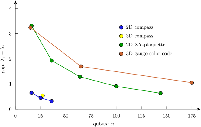
Figure 1: The spectral gap of four different gauge code Hamiltonians, versus the number of qubits $n$. The gap is defined as the difference between the ground eigenvalue and the first excited eigenvalue. These results are obtained by exact diagonalization.

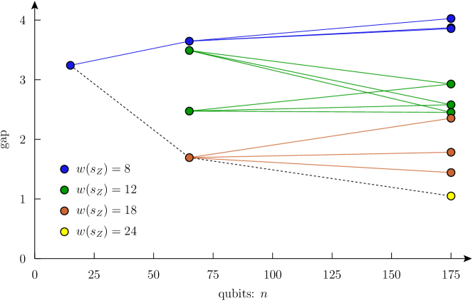
Figure 2: For the 3D gauge color code model we show the spectral gap of each Hamiltonian block $H_{t_{X},0}$ with $n=15,65,175.$ This gap is defined as $\lambda_{1}(H)-\lambda_{1}(H_{t_{X},0}).$ Each point is colored according to the weight of the frustrated stabilizer generator.

These numerics are shown in Figures 1 and 2. The gap of the 3D gauge color code is more robust than the other models, see Figure 1. It does decrease with $n$, but note also that the stabilizers in the code are also growing, up to weight 24. To emphasize this point we show in Figure 2 the ground eigenvalues of all of the blocks $H_{t_{X},0}.$ For larger codes in this family the stabilizers do not get bigger than weight 24. It is not clear to what extent these results are representative of larger code sizes, but we can already see from Figure 2 evidence that the weight of the frustrated stabilizer generator plays a more important role than the size of the code itself. In these examples, the gap always corresponds to frustrating a stabilizer ($t_{X}\neq 0$) and in particular the stabilizer generator with largest weight. This is a crucial connection to make because the stabilizers of the compass model (as well as the $XY$ and Ising models) grow with the linear size of the model while those of the gauge color code do not grow beyond a constant bound. This would suggest that if this is the mechanism for gapless behaviour that the gauge color code model may be gapped.

These numerical results reach the limit of presently available computational resources. To find eigenvalues for each Hamiltonian block $H_{t_{X},0}$ we need to operate on wavefunctions with $2^{r}$ real coefficients. The iterative solvers in SLEPc need to store at least two, but ideally more, of these wavefunctions. For $r=32$ this is about 32 Gigabytes for one wavefunction (using double precision coefficients) and so this value for $r$ is roughly the upper limit on these numerical techniques. Without decomposing the gauge color code into six disjoint ideals it would be impossible to obtain the results for the $n=175$ code, as this code has $r=94$.

6 Cheeger cuts

In this final section of this paper we give some heuristic arguments for why the size of the stabilizers is related to the gap of the Hamiltonian.

The Perron-Frobenius structure theory places strong constraints on the first and second eigenvectors of $\Gamma_{t_{X}}:$ the first eigenvector has all positive entries, and therefore all vectors orthogonal to the first eigenvector will have both positive and negative entries. In general, the set of edges of $\Gamma_{t_{X}}$ where such a vector changes sign we call a Cheeger cut [10, 11]. (We ignore the possibility that this vector may have zero entries.) The Cheeger cut associated to the second eigenvector is particularly important, and we next show an example of how this cut relates to the gap.

6.1 The double well model is gapless

We consider a linear graph Hamiltonian with a “double-well” potential. This does not correspond to any gauge code Hamiltonian. The state space will be $d$ dimensional with basis vectors numbered $|{1}\rangle,...,|{d}\rangle.$ We take $H=A+U$ with

$$A_{ij}=\left\{\begin{array}[]{ll}1&\mbox{if}\ |i-j|=1,\\ 0&\mbox{otherwise}\end{array}\right.\ \ \mbox{and}\ \ U_{ij}=\left\{\begin{array}[]{ll}2&\mbox{if}\ i=j=1\ \ \mbox{or}\ \ i=j=n,\\ 0&\mbox{otherwise.}\end{array}\right.$$

$A$ here is a kind of transition matrix, and $U$ is a diagonal potential energy term.

For $d\gg 1$, the largest eigenvalue is $\lambda_{1}\cong\frac{5}{2}$. The corresponding eigenvector $|{v_{1}}\rangle$ has all positive entries that decay exponentially away from the well sites at $|{1}\rangle$ and $|{d}\rangle:$

$$\langle{i}|{v_{1}}\rangle\cong 2^{i-1}\langle{1}|{v_{1}}\rangle\ \ \mbox{for}\ \ i\ll\frac{d}{2}.$$

For the second eigenvalue, $\lambda_{2}$ we also have $\lambda_{2}\cong\frac{5}{2}$ and indeed, as $d$ grows the gap $\lambda_{1}-\lambda_{2}\rightarrow 0$ and so this model is gapless.

Here we depict the wavefunctions for the first two eigenvectors for a system with $d=12:$

The simplest way to show this model is gapless is using a variational argument. Any another vector $|{u}\rangle$ that is orthogonal to the groundspace vector will have $\langle{u}|H|{u}\rangle\leq\lambda_{2}.$ To construct a candidate for $|{u}\rangle$ partition the basis vectors into two parts:

$$\Gamma=\Gamma_{A}\cup\Gamma_{B}$$

and write $|{v_{1}}\rangle=|{v_{A}}\rangle\oplus|{v_{B}}\rangle$ as well as Hamiltonian with this decomposition as

$$H=\left(\begin{array}[]{ll}H_{AA}&H_{AB}\\ H_{BA}&H_{BB}\end{array}\right).$$

Now let

$$|{u}\rangle=|{v_{A}}\rangle\oplus-|{v_{B}}\rangle$$

And then

$$\lambda_{2}\geq\langle{u}|H|{u}\rangle =\langle{v_{A}}|H_{AA}|{v_{A}}\rangle+\langle{v_{B}}|H_{BB}|{v_{B}}\rangle-\langle{v_{B}}|H_{BA}|{v_{A}}\rangle-\langle{v_{A}}|H_{AB}|{v_{B}}\rangle$$

$$=\lambda_{1}-4\langle{v_{B}}|H_{BA}|{v_{A}}\rangle.$$

So if we can show that $\langle{v_{B}}|H_{BA}|{v_{A}}\rangle$ tends to zero we are done. This term involves the dynamical coupling between the groundstate wavefunction along the cut between $A$ and $B$. To succeed we must find such a cut where the wavefunction is small. In general this appears to be quite difficult, even though in the models we are considering numerics show that not only is the wavefunction small away from potential wells but it is exponentially small.

6.2 The cut and symmetry

We now study the cut associated to the second eigenvector of a weakly self-dual gauge Hamiltonian $H,$ and relate this to the stabilizers of the code. The key realization is that $\Gamma_{t_{X}}$ is like the double well potential above, but now we have $2^{m_{X}}$ such wells, that is, one for every $s_{X}\in\langle S_{X}\rangle.$ This is clear from examining the basis vectors for $\Gamma_{t_{X}}.$ These are

$$|{vS_{X}+uR_{X}+t_{X}}\rangle,\ \ \mbox{where}\ \ v\in\mathcal{F}_{m_{X}},u\in\mathcal{F}_{r}$$

and those that satisfy the most $G_{Z}$ terms are precisely those with $u=0.$

We already know this is either the second eigenvector of $H_{0,0}$ or otherwise the first eigenvector of $H_{t_{X},0}$ for some $t_{X}\neq 0.$ To relate this to the Perron-Frobenius theory we note the decomposition from Lemma 3:

$$\Gamma_{t_{X}}=\bigoplus_{t_{Z}\in\langle T_{Z}\rangle}H_{t_{X},t_{Z}}.$$

This gives the spectral decomposition of each graph $\Gamma_{t_{X}}$ in terms of “momenta” $t_{Z}.$

We focus on $\Gamma_{0}.$ This must contain the second eigenvector of $H$ by weak self-duality of the code. $X$-type stabilizers $s_{X}\in S_{X}$ act on the $0,t_{Z}$ irreps in $\Gamma_{0}$ by $\pm 1$ according to the commutator $[[s_{X},t_{Z}]].$ Suppose the second eigenvector of $H$ lives in $H_{0,t_{Z}}$ for $t_{Z}\neq 0$. Let $s_{X}\in S_{X}$ with $[[s_{X},t_{Z}]]=-1.$ Then we must have an odd number of Cheeger cuts on every $\Gamma_{0}$ path between $|{v}\rangle$ and $s_{X}|{v}\rangle$ for all basis vectors $|{v}\rangle,$ that is, $v\in\langle S_{X}\rangle\oplus\langle R_{X}\rangle.$

In a similar vein, if the second eigenvector of $H$ lives in $H_{0,0}$ then we must have an even number of Cheeger cuts on every $\Gamma_{0}$ path between $|{v}\rangle$ and $s_{X}|{v}\rangle$ for all stabilizers $s_{X}\in S_{X}$ and basis vectors $|{v}\rangle.$

In summary, the idea is that large stabilizers lead to widely separated well potentials and hence gapless behaviour, while stabilizers of bounded weight force the cuts to appear close to the wells and hence maintain a gap. Even though numerics show the wavefunction becoming exponentially small away from well potentials, it is also exponentially wide. So making these arguments rigorous appears to be difficult.

The following fact would appear to be true under certain conditions, but is not at all true for example when $T$ is trivial:

Proto-fact: For a sufficiently “well-behaved” weakly self-dual gauge code Hamiltonian $H$

$$\lambda_{2}(H) =\min_{t_{X}\neq 0}\lambda_{1}(H_{t_{X},0})$$

$$=\min_{t_{Z}\neq 0}\lambda_{1}(H_{0,t_{Z}}).$$

Indeed, contrary to this proto-fact we suspect that $H_{0,0}$ will not be gapped in the generic case. Numerics suggest that there is no lower bound on the gap of randomly constructed stabilizer-less gauge code Hamiltonians. Perhaps double well behaviour can still be imitated even without stabilizers: merely having a large region of almost-stabilizer behaviour (large shallow well) could be enough to send the gap to zero.

6.3 Cheeger inequalities

We saw above how the Cheeger cut gives a variational ansatz for building a second eigenvector to the Hamiltonian and hence an upper bound on the gap. In this section we show how the Cheeger cut also yields a lower bound on the gap.

In [12], they derive the following Cheeger inequality by considering bi-partitions of the graph. We will do the same, but using matrix block notation.

Let $v_{2}$ be a second eigenvector, $Hv_{2}=\lambda_{2}v_{2}$ and $||v_{2}||=1$. We bi-partition the space so that $v_{2}$ has (vector) blocks:

$$v_{2}=\left(\begin{array}[]{l}x\\ y\end{array}\right)\quad$$

with $x\geq 0$ and $y\leq 0,$ entry-wise. Let the blocks of $H$ under the same partition be:

$$H=\left(\begin{array}[]{ll}A&C\\ C^{\top}&B\end{array}\right).\quad$$

If we denote $\lambda_{1}(A)$ as the top eigenvalue of $A$ and $\lambda_{1}(B)$ as the top eigenvalue of $B$, then

$$\lambda_{2}=v_{2}^{\top}Hv_{2} =x^{\top}Ax+2x^{\top}Cy+y^{\top}By$$

$$\leq x^{\top}Ax+y^{\top}By\ \leq\ ||x||^{2}\lambda_{1}(A)+||y||^{2}\lambda_{1}(B)$$

$$\leq\mbox{min}(\lambda_{1}(A),\lambda_{1}(B))\ \leq\ \lambda_{1}.$$

Defining the following constant as a maximization over all bi-partitions of $H:$

$$\nu(H):=\max_{A,B}\ \mbox{min}(\lambda_{1}(A),\lambda_{1}(B))$$

the above calculation shows that

$$\lambda_{2}\leq\nu(H)\leq\lambda_{1}.$$

7 Discussion

The goal of this paper is to understand the spectra of certain frustrated qubit Hamiltonians. Of particular interest is to understand how the gap between the first two eigenvalues behaves as we increase the number of qubits. For a system to maintain a topologically ordered groundstate we would expect this gap to be bounded away from zero, or gapped.

The numerical results obtained show some evidence for this gapped behaviour for the 3D gauge color code Hamiltonian. To get these numerics we rely on several key results. The first is to decompose the Hamiltonian into a direct sum of operators labelled by stabilizer eigenvalues. This is essentially group representation theory as applied to gauge codes. The second result was obtained using Perron-Frobenius theory, as the Hamiltonians of interest are stoquastic. This theory shows where the first and second eigenvalue is to be found in the block decomposition of the Hamiltonian, which leads to a polynomial reduction in the numeric workload. The third key result is the decomposition of each Hamiltonian block into mutually commuting ideals. In the case of the 3D gauge color code Hamiltonian, this decomposition yields an exponential reduction in the numeric workload, by dividing the number of qubits by six.

Finally, the connection between stabilizer size and the gap is further investigated via the idea of the Cheeger cut. This builds on the Perron-Frobenius theory results. If the groundstate wavefunction is sufficiently concentrated into potential wells, then we can construct an excited state that has eigenvalue close to the ground eigenvalue. And the distance between potential wells is controlled by the size of stabilizers. The conjecture we would like to make would state how this spectral gap is controlled by the size of the frustrated stabilizers: large stabilizers lead to gappless behaviour while small stabilizers maintain a gap. However, it is not clear how to formulate this conjecture, and even less clear how to prove it. More numerics need to be performed, with the specific goal of understanding the shape of the groundspace wavefunction, and how this relates to the geometry of the underlying code.

References

- [1] D. Bacon. Operator quantum error-correcting subsystems for self-correcting quantum memories. Phys. Rev. A, 73:012340, Jan 2006.
- [2] J. C. Baez and J. Biamonte. Quantum techniques for stochastic mechanics. arXiv preprint arXiv:1209.3632, 2012.
- [3] H. Bombín. Gauge color codes: optimal transversal gates and gauge fixing in topological stabilizer codes. New Journal of Physics, 17(8):083002, 2015.
- [4] H. Bombín. Single-shot fault-tolerant quantum error correction. Physical Review X, 5(3):031043, 2015.
- [5] H. Bombin and M. Martin-Delgado. Exact topological quantum order in d= 3 and beyond: Branyons and brane-net condensates. Physical Review B, 75(7):075103, 2007.
- [6] S. Bravyi. Monte carlo simulation of stoquastic hamiltonians. Quantum Information & Computation, 15(13–14):1122–1140, 2015.
- [7] S. Bravyi, D. P. Divincenzo, R. Oliveira, and B. M. Terhal. The complexity of stoquastic local hamiltonian problems. Quantum Information & Computation, 8(5):361–385, 2008.
- [8] B. J. Brown, D. Loss, J. K. Pachos, C. N. Self, and J. R. Wootton. Quantum memories at finite temperature. Rev. Mod. Phys., 88:045005, Nov 2016.
- [9] W. Brzezicki and A. M. Oleś. Symmetry properties and spectra of the two-dimensional quantum compass model. Phys. Rev. B, 87:214421, Jun 2013.
- [10] J. Cheeger. A lower bound for the smallest eigenvalue of the laplacian. Problems in analysis, pages 195–199, 1970.
- [11] F. R. Chung. Spectral graph theory. Number 92. American Mathematical Soc., 1997.
- [12] S. Friedland and R. Nabben. On cheeger-type inequalities for weighted graphs. Journal of Graph Theory, 41(1):1–17, 2002.
- [13] F. G. Frobenius. Über matrizen aus nicht negativen elementen. 1912.
- [14] V. Hernandez, J. E. Roman, and V. Vidal. SLEPc: A scalable and flexible toolkit for the solution of eigenvalue problems. ACM Trans. Math. Software, 31(3):351–362, 2005.
- [15] A. Y. Kitaev. Fault-tolerant quantum computation by anyons. Ann. Phys., 303(1):2–30, 2003.
- [16] A. Kubica, B. Yoshida, and F. Pastawski. Unfolding the color code. New Journal of Physics, 17(8):083026, 2015.
- [17] E. Lieb, T. Schultz, and D. Mattis. Two soluble models of an antiferromagnetic chain. Annals of Physics, 16(3):407–466, 1961.
- [18] O. Perron. Zur theorie der matrices. Mathematische Annalen, 64(2):248–263, 1907.
- [19] P. Pfeuty. The one-dimensional ising model with a transverse field. ANNALS of Physics, 57(1):79–90, 1970.