Generalized Linear Models with Linear Constraints for Microbiome Compositional Data

Abstract

Motivated by regression analysis for microbiome compositional data, this paper considers generalized linear regression analysis with compositional covariates, where a group of linear constraints on regression coefficients are imposed to account for the compositional nature of the data and to achieve subcompositional coherence. A penalized likelihood estimation procedure using a generalized accelerated proximal gradient method is developed to efficiently estimate the regression coefficients. A de-biased procedure is developed to obtain asymptotically unbiased and normally distributed estimates, which leads to valid confidence intervals of the regression coefficients. Simulations results show the correctness of the coverage probability of the confidence intervals and smaller variances of the estimates when the appropriate linear constraints are imposed. The methods are illustrated by a microbiome study in order to identify bacterial species that are associated with inflammatory bowel disease (IBD) and to predict IBD using fecal microbiome.

1 Introduction

Human micorbiome consists of all living microorganisms that are in and on human body. These micro-organisms have been shown to be associated with complex diseases and to influence our health. Advanced sequencing technologies such as 16S sequencing and shotgun metagenomic sequencing, provide powerful methods to quantify the relative abundance of bacterial taxa in large samples. Since only the relative abundances are available, the resulting data are compositional with a unit sum constraint. The compositional nature of the data requires additional care in statistical analysis, including linear regression analysis (Lin et al., 2014; Shi et al., 2016; Aitchison and Bacon-shone, 1984).

The main challenges of analyzing compositional data are to account for the unit sum structure and to achieve subcompositional coherence (Aitchison, 1982), which requires that the same results are obtained regardless of the way the data is normalized based on the whole compositions or only a subcomposition. To explore the association between outcome and the compositional data, Aitchison and Bacon-shone (1984) proposed a linear log-contrast model to link the outcome and the log of the compositional data. Lin et al. (2014) further developed this model and considered variable selection by a $\ell_{1}$-penalized estimation procedure. To achieve subcompositional coherence, Shi et al. (2016) extended the linear regression model by imposing a set of linear constraints. The log-contrast model and its extensions are suitable when the outcome variable is continuous and normal distributed.

In this paper, the generalized linear regression models (GLMs) with linear constraints in the regression coefficients are proposed for microbiome compositional data, where a group of linear constraints are imposed to achieve subcompositional coherence. In order to identify the bacterial taxa that are associated with the outcome, a penalized estimation procedure for the regression coefficients via a $\ell_{1}$ penalty is introduced. To solve the computational problem, a generalized accelerated proximal gradient method is developed, which extends the standard accelerated proximal gradient method (Nesterov, 2013) to account for linear constraints. The proposed method can efficiently solve the optimization problem of minimizing the penalized negative log-likelihood subjects to a group of linear constraints.

Previous works on the inference of Lasso for the generalized linear models include Bühlmann and Van De Geer (2011), who provided properties of the penalized estimates such as bound for $\ell_{1}$ loss and oracle inequality. However, the methods cannot be applied directly to the setting with linear constraints. Furthermore, it is known that the $\ell_{1}$ penalized estimates are biased and do not have a tractable asymptotic distribution. In order to correct such biases, works have been done for the Lasso estimate, including Zhang and Zhang (2014), who proposed a low-dimensional projection estimator to correct the bias and Javanmard and Montanari (2014), who used a quadratic programming method to carry out the task. Van de Geer et al. (2014) considers an extension to generalized linear models. However, these methods still cannot be directly applied to our problem due to the linear constraints.

In order to make statistical inference on the regression coefficients, we propose a bias correction procedure for GLMs with linear constraints by extending the method of Javanmard and Montanari (2014). Such a debiased procedure provides asymptotically unbiased and normal distributed estimates of the regression coefficients, which can be used to construct confidence intervals. Our simulations results show the correctness of the coverage probability of the confidence intervals and smaller variances of the estimates when the appropriate linear constraints are imposed.

Section 2 develops the GLMs for compositional data and provides an efficient algorithm to solve the optimization problem. Section 3 provides a de-biased procedure to correct the biases of the penalized estimates and derives the asymptotic distribution of the de-biased estimates. Section 4 presents the result of identifying gut bacterial species that are associated with inflammatory bowel disease. Section 5 provides the simulation results that illustrate the correctness of the proposed method. Some discussion and suggestion for future work are provided in Section 6. Proofs of the theorems are included in the Appendix.

2 GLMs with Linear Constraints for Microbiome Compositional Data

2.1 GLMs with linear constraints

Consider a microbiome study with outcome $y_{i}$ and a $p$ dimensional compositional covariates $\mathbf{X}_{i}=(x_{i1},\cdots,x_{ip})$ with the unit sum constraint $\sum_{j}x_{ij}=1$ for $i=1,\cdots,n$, where $x_{ij}$ represents the relative abundance of the $j$th taxon for the $i$th samples. To account for compositional nature of the covariates, Lin et al. (2014) proposed the linear model with constraint:

$$y_{i}=\mathbf{Z}_{i}^{\top}{\boldsymbol{\beta}}+\epsilon_{i},\mbox{ subject to }C^{\top}{\boldsymbol{\beta}}=0$$ (1)

where $\mathbf{Z}_{i}=\{\log(x_{ij})\}\in{\mathbb{R}}^{n\times p}$ and $C=(1,1,\ldots,1)^{\top}$. Shi et al. (2016) further developed this method to allow multiple linear constraints by specifying the $p\times r$ constraint matrix $C$. Such constraints ensure that the regression coefficients are independent of an arbitrary scaling of the basis from which a composition is obtained, and remain unaffected by correctly excluding some or all of the zero components. This subcompositional coherence property is one of the principals of compositional data analysis (Aitchison, 1982).

For general outcome, we extend the linear model (1) to the generalized linear model with its density function specidied as

$$\begin{split}f(y_{i}|{\boldsymbol{\beta}},\mathbf{Z}_{i})=h(y_{i})\exp\left\{\eta_{i}y_{i}-A(\eta_{i})\right\},\quad\eta_{i}=\mathbf{Z}_{i}^{\top}{\boldsymbol{\beta}}\\ {\mathbb{E}}y_{i}=\triangledown_{\eta_{i}}A(\eta_{i})\equiv\mu({\boldsymbol{\beta}},\mathbf{Z}_{i}),\quad{\rm Var}y_{i}=\triangledown_{\eta_{i}}^{2}A(\eta_{i})\equiv v({\boldsymbol{\beta}},\mathbf{Z}_{i})\\ \end{split}$$ (2)

where ${\boldsymbol{\beta}}=(\beta_{1},\beta_{2},\ldots\beta_{p})^{\top}\in{\mathbb{R}}^{p}$ and satisfies

$$C^{\top}{\boldsymbol{\beta}}=0,$$

and $\mathbf{Z}_{i}^{\top}=(Z_{i1},Z_{i2},\ldots,Z_{ip})$. For simplicity, we assume the intercept being zero, though our formal justification will allow for an intercept. For binary outcome and logistic regression, we have

$$A(\eta)=\log(1+e^{\eta}),\mu({\boldsymbol{\beta}},\mathbf{Z}_{i})=\dfrac{e^{\mathbf{Z}_{i}^{\top}{\boldsymbol{\beta}}}}{1+e^{\mathbf{Z}_{i}^{\top}{\boldsymbol{\beta}}}},v({\boldsymbol{\beta}},\mathbf{Z}_{i})=\dfrac{e^{\mathbf{Z}_{i}^{\top}{\boldsymbol{\beta}}}}{(1+e^{\mathbf{Z}_{i}^{\top}{\boldsymbol{\beta}}})^{2}}.$$

2.2 $\ell_{1}$ penalized estimation with constraints

The log-likelihood function based on model (2) is given by

$$\ell({\boldsymbol{\beta}}|{\mathbf{Y}},\mathbf{Z}) =\sum_{i=1}^{n}\log h(y_{i})+{\mathbf{Y}}^{\top}\mathbf{Z}{\boldsymbol{\beta}}-\sum_{i=1}^{n}A(\mathbf{Z}_{i}^{\top}{\boldsymbol{\beta}}),$$ (3)

with score function and information matrix:

$$\triangledown_{{\boldsymbol{\beta}}}\ell({\boldsymbol{\beta}}|{\mathbf{Y}},\mathbf{Z})=({\mathbf{Y}}-\boldsymbol{\mu}({\boldsymbol{\beta}},\mathbf{Z}))^{\top}\mathbf{Z},\mbox{ }\triangledown_{{\boldsymbol{\beta}}}^{2}\ell({\boldsymbol{\beta}}|{\mathbf{Y}},\mathbf{Z})=-\mathbf{Z}^{\top}\mathbf{V}({\boldsymbol{\beta}},\mathbf{Z})\mathbf{Z},$$

where $\mathbf{V}({\boldsymbol{\beta}},\mathbf{Z})={\rm diag}\{v({\boldsymbol{\beta}},Z_{1}),\dots,v({\boldsymbol{\beta}},Z_{n})\}$. The constraints on ${\boldsymbol{\beta}}$ are given by $C^{\top}{\boldsymbol{\beta}}=0$, where $C$ is a $p\times r$ matrix. Without lose of generality, the columns of $C$ are assumed to be orthonormal. Define $P_{C}=CC^{\top}$, $\widetilde{\mathbf{Z}}=\mathbf{Z}(\mathbf{I}_{p}-P_{C})$ and $\widetilde{Z}_{i}=(\mathbf{I}_{p}-P_{C})\mathbf{Z}_{i}$, then under the constraints of $C^{\top}{\boldsymbol{\beta}}=0$, all the $\mathbf{Z}$ and $Z_{i}$ can be replaced by $\widetilde{\mathbf{Z}}$ and $\widetilde{Z}_{i}$ because $\mathbf{Z}{\boldsymbol{\beta}}=\widetilde{\mathbf{Z}}{\boldsymbol{\beta}}$.

In high-dimensional settings, ${\boldsymbol{\beta}}$ is assumed to be $s$-sparse, where $s=\#\{i:{\boldsymbol{\beta}}_{i}\neq 0\}$ and $s=o(\sqrt{n}/\log p)$. The $\ell_{1}$ penalized estmates of ${\boldsymbol{\beta}}$ is given as the solution to the following problem:

$$\hat{{\boldsymbol{\beta}}}^{n}=\operatorname*{argmin}_{{\boldsymbol{\beta}}}\left\{-\dfrac{1}{n}[{\mathbf{Y}}^{\top}\widetilde{\mathbf{Z}}{\boldsymbol{\beta}}-\sum_{i=1}^{n}A(\widetilde{\mathbf{Z}}_{i}^{\top}{\boldsymbol{\beta}})]+\lambda||{\boldsymbol{\beta}}||_{1}\right\}\mbox{ subject to }C^{\top}{\boldsymbol{\beta}}=0,$$ (4)

where $\lambda$ is a tuning parameter.

2.3 Generalized accelerated proximal gradient method

Due to the linear constraints in the optimization problem (4), the standard coordinate descent algorithm cannot be applied directly. We develop a generalized accelerated proximal gradient algorithm. Specifically, define $g,h$ as following

$$g({\boldsymbol{\beta}})=-\dfrac{1}{n}[Y^{\top}\widetilde{\mathbf{Z}}{\boldsymbol{\beta}}-\sum_{i=1}^{n}A(\widetilde{Z}_{i}^{\top}{\boldsymbol{\beta}})],\quad h({\boldsymbol{\beta}})=\lambda||{\boldsymbol{\beta}}||_{1}$$

so the optimization problem (4) becomes

$$\hat{{\boldsymbol{\beta}}}^{n}=\operatorname*{argmin}_{{\boldsymbol{\beta}}}\left\{g({\boldsymbol{\beta}})+h({\boldsymbol{\beta}})\right\}\mbox{ subject to }C^{\top}{\boldsymbol{\beta}}=0.$$

Since $g$ is convex and differentiable and $h$ is convex, the standard accelerated proximal gradient method (Nesterov, 2013) is given by the following iterations:

$${\boldsymbol{\beta}}^{(k)}=\textbf{prox}_{t_{k}h}\left(y^{(k-1)}-t_{k}\nabla g(y^{(k-1)})\right),$$

$$y^{(k)}={\boldsymbol{\beta}}^{(k)}+\frac{k-1}{k+r-1}({\boldsymbol{\beta}}^{(k)}-{\boldsymbol{\beta}}^{(k-1)}),$$

where $t_{k}$ is the step size in the $k$-th iteration and $r$ is a friction parameter. The proximal mapping of a convex function $h$, which is the key ingredient of this algorithm, is defined as:

$$\textbf{prox}_{h}(x)=\operatorname*{argmin}_{u}\left\{h(u)+\frac{1}{2}||x-u||^{2}_{2}\right\}.$$

We generalize this method to handle the linear constraints. Denote $S_{C}=\{{\boldsymbol{\beta}}\in{\mathbb{R}}^{p}\ |\ C^{\top}{\boldsymbol{\beta}}=0\}$, a linear subspace of ${\mathbb{R}}^{p}$. The generalized accelerated proximal gradient method becomes

$${\boldsymbol{\beta}}^{(k)}=\operatorname*{argmin}_{{\boldsymbol{\beta}}\in S_{C}}\left\{\lambda t_{k}\|{\boldsymbol{\beta}}\|_{1}+\frac{1}{2}||y^{(k-1)}-t_{k}\nabla g(y^{(k-1)})-{\boldsymbol{\beta}}||^{2}_{2}\right\},$$ (5)

$$y^{(k)}={\boldsymbol{\beta}}^{(k)}+\frac{k-1}{k+r-1}({\boldsymbol{\beta}}^{(k)}-{\boldsymbol{\beta}}^{(k-1)}).$$ (6)

The minimization of (5) can be solved by soft thresholding and projection:

$${\boldsymbol{\beta}}^{(k)}=\Pi_{S_{C}}\left(S_{t_{k}\lambda}\left(y^{(k-1)}-t_{k}\nabla g(y^{(k-1)})\right)\right),$$

where linear operator $\Pi_{S_{C}}(u)$ projects $u$ onto space $S_{C}$. Since $C^{\top}$ is a matrix and can be regarded as a linear mapping from $R^{p}\mapsto R^{r}$, we have $S_{C}=\ker(C^{\top})$. Denote $u_{p}=\Pi_{S_{C}}(u)$, we have:

$$C^{\top}(u-u_{p})=C^{\top}u$$

So $u-u_{p}$ is given by least square estimates: $u-u_{p}=(CC^{\top})^{\dagger}CC^{\top}u$, where $A^{\dagger}$ is the Moore-Penrose pseudo inverse of a matrix $A$. Hence,

$$\Pi_{S_{C}}(u)=u-(CC^{\top})^{\dagger}CC^{\top}u.$$

The step size $t_{k}$ can be fixed or chosen by line search. The procedure of line search consists of the following iterations: we start with a initial $t=t_{k-1}$ and repeat $t=0.5t$ until the following inequality holds:

$$g(y-tG_{t}(y))\leq g(y)-t\nabla g(y)^{\top}G_{t}(y)+\frac{t}{2}\|G_{t}(y)\|_{2}^{2}$$

where $y=y^{(k-1)}$. For the friction parameter $r$, Su et al. (2014) suggested that $r>4.5$ will lead to fast convergence rate and is set to 10.

3 De-biased Estimator and its Asymptotic Distribution

We collect here the notations used in the rest of the paper. For a vector ${\boldsymbol{x}}$, $\|{\boldsymbol{x}}\|_{p}$ is the standard $\ell_{p}$-norm. For a matrix ${\mathbf{A}}_{m\times n}$, $\|{\mathbf{A}}\|_{p}$ is the $\ell_{p}$ operator norm defined as $\|{\mathbf{A}}\|_{p}=\sup_{\|x\|_{p}=1}\|{\mathbf{A}}{\boldsymbol{x}}\|_{p}$. In particular, $\|{\mathbf{A}}\|_{\infty}=\max_{1\leq i\leq m}\sum_{j=1}^{n}|a_{ij}|$ and $|{\mathbf{A}}|_{\infty}$ is defined as $|{\mathbf{A}}|_{\infty}=\max_{i,j}|a_{ij}|$. For square matrix ${\mathbf{A}}$, denote $\sigma_{\textrm{max}}({\mathbf{A}})(\sigma_{\textrm{min}}(A))$ is the largest (smallest) non-zero eigenvalue of ${\mathbf{A}}$.

3.1 A de-biased Estimator

Since $\widehat{{\boldsymbol{\beta}}}^{n}$ in equation (4) is a biased estimator for ${\boldsymbol{\beta}}$ due to $\ell_{1}$ penalization, we propose the following de-biased procedure, detailed as Algorithm 1, to obtain asymptotically unbiased estimates of ${\boldsymbol{\beta}}$.

Algorithm 1 Constructing a de-biased estimator

Input: ${\mathbf{Y}}$, $\mathbf{Z}$, $\widehat{{\boldsymbol{\beta}}}^{n}$, and $\gamma$. Output: $\widehat{{\boldsymbol{\beta}}}^{u}$

1:Let $\widehat{{\boldsymbol{\beta}}}^{n}$ be the regularized estimator from optimization problem (4).

2:Set $\widetilde{\mathbf{Z}}=\mathbf{Z}(\mathbf{I}_{p}-P_{C})$, $\widehat{{\boldsymbol{\Sigma}}}=(\widetilde{\mathbf{Z}}^{\top}\mathbf{V}(\hat{{\boldsymbol{\beta}}}^{n},\widetilde{\mathbf{Z}})\widetilde{\mathbf{Z}})/n$.

3:for $i=1,2,\dots,p$ do

4:Let $m_{i}$ be a solution of the convex program:

$$\begin{split}\mbox{minimize }&m^{\top}\widehat{{\boldsymbol{\Sigma}}}m\\ \mbox{subject to }&||\widehat{{\boldsymbol{\Sigma}}}m-(\mathbf{I}_{p}-P_{C})e_{i}||_{\infty}\leq\gamma.\\ \end{split}$$ (7)

where $e_{i}\in{\mathbb{R}}^{p}$ is the vector with one at the $i$-th position and zero everywhere else.

5:Set $M=(m_{1},\dots,m_{p})^{\top}$, set

$$\widetilde{M}=(\mathbf{I}_{p}-P_{C})M.$$ (8)

6:Define the estimator $\widehat{{\boldsymbol{\beta}}}^{u}$ as follows:

$$\widehat{{\boldsymbol{\beta}}}^{u}=\widehat{{\boldsymbol{\beta}}}^{n}+\dfrac{1}{n}\widetilde{M}\widetilde{\mathbf{Z}}^{\top}({\mathbf{Y}}-\boldsymbol{\mu}(\widehat{{\boldsymbol{\beta}}}^{n},\widetilde{\mathbf{Z}})).$$ (9)

From the construction of $\hat{{\boldsymbol{\beta}}}^{u}$, it is easy to check that $\hat{{\boldsymbol{\beta}}}^{u}$ still satisfies $C^{\top}\hat{{\boldsymbol{\beta}}}^{u}=0$. To provide insights into this algorithm, using the mean value theorem, there exists ${\boldsymbol{\beta}}_{i}^{0}$ such that

$$\mu(\hat{{\boldsymbol{\beta}}}^{n},\mathbf{Z}_{i})-\mu({\boldsymbol{\beta}},\mathbf{Z}_{i})=v({\boldsymbol{\beta}}_{i}^{0},\mathbf{Z}_{i})\mathbf{Z}_{i}^{\top}(\hat{{\boldsymbol{\beta}}}^{n}-{\boldsymbol{\beta}}),\ i=1,2,\ldots,n.$$

Define $\widehat{{\boldsymbol{\Sigma}}}^{0}=(\widetilde{\mathbf{Z}}^{\top}\mathbf{V}({\boldsymbol{\beta}}^{0},\widetilde{\mathbf{Z}})\widetilde{\mathbf{Z}})/n$, where $\mathbf{V}({\boldsymbol{\beta}}^{0},\widetilde{\mathbf{Z}})={\rm diag}\{v({\boldsymbol{\beta}}_{1}^{0},Z_{1}),\dots,v({\boldsymbol{\beta}}_{n}^{0},Z_{n})\}$, we have

$$\sqrt{n}\left(\hat{{\boldsymbol{\beta}}}^{u}-{\boldsymbol{\beta}}\right) =\sqrt{n}[(\mathbf{I}_{p}-P_{C})-\widetilde{M}\widehat{{\boldsymbol{\Sigma}}}^{0}](\hat{{\boldsymbol{\beta}}}^{n}-{\boldsymbol{\beta}})+\dfrac{1}{\sqrt{n}}\widetilde{M}\widetilde{\mathbf{Z}}^{\top}(Y-\boldsymbol{\mu}({\boldsymbol{\beta}},\widetilde{\mathbf{Z}})) *$$ ()

$$\equiv\Delta+R.$$

Define ${\boldsymbol{\Sigma}}=(\widetilde{\mathbf{Z}}^{\top}\mathbf{V}({\boldsymbol{\beta}},\widetilde{\mathbf{Z}})\widetilde{\mathbf{Z}})/n$ and ${\boldsymbol{\Sigma}}_{{\boldsymbol{\beta}}}={\mathbb{E}}{\boldsymbol{\Sigma}}={\mathbb{E}}(v({\boldsymbol{\beta}},\widetilde{Z}_{1})\widetilde{Z}_{1}\widetilde{Z}_{1}^{\top})$, and suppose ${\boldsymbol{\Sigma}}_{{\boldsymbol{\beta}}}=V_{{\boldsymbol{\beta}}}\Lambda_{{\boldsymbol{\beta}}}V_{{\boldsymbol{\beta}}}^{\top}$ is the eigenvalue decomposition of ${\boldsymbol{\Sigma}}_{{\boldsymbol{\beta}}}$. Since $(V_{{\boldsymbol{\beta}}},C)$ is full rank and orthonormal, we have

$${\boldsymbol{\Sigma}}_{{\boldsymbol{\beta}}}=(V_{{\boldsymbol{\beta}}},C)\left(\begin{array}[]{cc}\Lambda&0\\ 0&0\end{array}\right)(V_{{\boldsymbol{\beta}}},C)^{\top},\mbox{ }\Omega_{{\boldsymbol{\beta}}}=(V_{{\boldsymbol{\beta}}},C)\left(\begin{array}[]{cc}\Lambda_{{\boldsymbol{\beta}}}^{-1}&0\\ 0&0\end{array}\right)(V_{{\boldsymbol{\beta}}},C)^{\top},$$

which implies

$${\boldsymbol{\Sigma}}_{{\boldsymbol{\beta}}}\Omega_{{\boldsymbol{\beta}}}=(V_{{\boldsymbol{\beta}}},C)\left(\begin{array}[]{cc}\mathbf{I}_{p-r}&0\\ 0&0\end{array}\right)(V_{{\boldsymbol{\beta}}},C)^{\top}=V_{{\boldsymbol{\beta}}}V_{{\boldsymbol{\beta}}}^{\top}=\mathbf{I}_{p}-P_{C}.$$

So Step 4 of Algorithm 1 approximates $\Omega_{{\boldsymbol{\beta}}}$ by rows.

3.2 Asymptotic distribution

In order to derive the asymptotic distribution of the de-biased estimator $\hat{{\boldsymbol{\beta}}}^{u}$, several regularity conditions are required.

1. $\|\mathbf{I}_{p}-P_{C}\|_{\infty}\leq k_{0}$ for a constant $k_{0}$ that is free of $p$.

2. The diagonal elements of $\mathbf{I}_{p}-P_{C}$ are greater than zero.

Conditions C1 and C2 have been used in Shi et al. (2016) and naturally hold in our setting as well. In addition, define $\widetilde{\mathbf{Z}}^{*}=D\widetilde{\mathbf{Z}}$, where $D\in\widetilde{D}_{ab}$ is defined as:

$$\widetilde{D}_{ab}=\{D\in{\mathbb{R}}^{n\times n}:{\rm diag}(d_{1},d_{2},\ldots,d_{n}),a\leq d_{i}\leq b,\,0<a<b\}.$$

For any matrix $A\in{\mathbb{R}}^{n\times m}$, the upper and lower restricted isometry property (RIP) constant of order $k$, $\delta_{k}^{+}(A)$ and $\delta_{k}^{-}(A)$, are defined as:

$$\delta_{k}^{+}(A)=\sup\left(\dfrac{\|A\alpha\|_{2}^{2}}{\|\alpha\|_{2}^{2}}:\ \alpha\in{\mathbb{R}}^{m}\ \textrm{is $k$-sparse vector}\right),$$

$$\delta_{k}^{-}(A)=\inf\left(\dfrac{\|A\alpha\|_{2}^{2}}{\|\alpha\|_{2}^{2}}:\ \alpha\in{\mathbb{R}}^{m}\ \textrm{is $k$-sparse vector}\right).$$

We assume the following RIP condition:

1. [3.]

2. $\inf_{\widetilde{D}_{01}}\left((3\tau-1)\delta_{2s}^{-}(\widetilde{\mathbf{Z}}^{*}/\sqrt{n})-(\tau+1)\delta_{2s}^{+}(\widetilde{\mathbf{Z}}^{*}/\sqrt{n})\right)\geq 4\tau\phi_{0}$ for some constant $\phi_{0}$.

Condition C3 is slightly stronger than the one used for linear regression, which here we require the inequality holds uniformly over a set of matrices. The following theorem quantifies the difference between $\hat{{\boldsymbol{\beta}}}^{n}$ and ${\boldsymbol{\beta}}$ in $\ell_{1}$ norm.

Theorem 3.1

Let $\hat{{\boldsymbol{\beta}}}^{n}$ be the solution for (4), where ${\boldsymbol{\beta}}$ is $s$-sparse. If Conditions C1-C3 hold, and the tuning parameter $\lambda=\tau\tilde{c}\sqrt{(\log p)/n}$, then

$${\mathbb{P}}\left(\|\hat{{\boldsymbol{\beta}}}^{n}-{\boldsymbol{\beta}}\|_{1}\geq\dfrac{s\lambda(k_{0}+1/\tau)}{\phi_{0}}\right)\leq 2p^{-c^{\prime}}$$

where $c^{\prime}=\dfrac{\tilde{c}^{2}}{2K^{2}}-1$ and $K=\max_{i}\sqrt{(\widetilde{\mathbf{Z}}^{\top}\widetilde{\mathbf{Z}}/n)_{i,i}}$.

In order to establish the asymptotic distribution of the de-biased estimates, additional conditions are required:

1. There exist uniform constants $C_{\text{min}}$ and $C_{\text{max}}$ such that $0<C_{\text{min}}\leq\sigma_{\textrm{min}}({\boldsymbol{\Sigma}}_{{\boldsymbol{\beta}}})\leq\sigma_{\textrm{max}}({\boldsymbol{\Sigma}}_{{\boldsymbol{\beta}}})\leq C_{\text{max}}<\infty$.

2. $|\Omega_{{\boldsymbol{\beta}}}\Theta|_{\infty}<\infty$.

3. The variance function $v({\boldsymbol{\beta}},\mathbf{Z}_{i})$ satisfies Lipschitz condition with constant $C$;

4. There exists a uniform constant $\kappa>0$ such that $\|\Omega^{1/2}\widetilde{Z}_{k}\|_{\psi_{2}}\leq\kappa$ for all $k=1,\ldots,n$.

In Condition C7, the sub-Gaussian norm of a random vector $Z\in{\mathbb{R}}^{n}$ is defined as

$$\|Z\|_{\psi_{2}}=\sup\left(\|Z^{\top}x\|_{\psi_{2}}:\ x\in{\mathbb{R}}^{n}\,\text{and}\,\|x\|_{2}=1\right),$$

and the sub-Gaussian norm for a random variable $X$, is defined as

$$\|X\|_{\psi_{2}}=\sup_{q\geq 1}q^{-1/2}({\mathbb{E}}|X|^{q})^{1/q}.$$

Conditions C4 and C7 are bounded eigenvalue assumption and bounded sub-Gaussian norm that are widely used in the literature of inference with respect to Lasso type estimator (Shi et al., 2016; Javanmard and Montanari, 2014). Condition C5 eliminates extreme situations on $|\Omega_{{\boldsymbol{\beta}}}\Theta|_{\infty}$, which actually can be relaxed to hold in probability. For logistic regression, similar conditions are used in Ning et al. (2017). Condition C6 is a Lipschitz condition on the variance function, which holds for many of the GLMs including logistic regression.

The following Lemma shows that if the tuning parameter $\gamma$ in the optimization problem (7) is chosen to be $c\sqrt{(\log p)/n}$, then $\Omega_{{\boldsymbol{\beta}}}$ is in the feasible set with a large probability.

Lemma 3.2

Denote $\Theta={\mathbb{E}}\widetilde{Z}_{1}\widetilde{Z}_{1}^{\top}$. Suppose Conditions C1-C7 hold, then for any constant $c>0$, the following inequality holds:

$${\mathbb{P}}\left(|\bm{\Omega}_{{\boldsymbol{\beta}}}\widehat{{\boldsymbol{\Sigma}}}-(\mathbf{I}_{p}-P_{C})|_{\infty}\geq c\sqrt{(\log p)/n}\right)\leq 2p^{-c_{1}^{{}^{\prime\prime}}}+2p^{-c_{2}^{{}^{\prime\prime}}}$$

where $c_{1}^{{}^{\prime\prime}}=c^{2}C_{\text{min}}/(24e^{2}C_{\text{max}}\kappa^{4})-2$ and $c_{2}^{{}^{\prime\prime}}=\hat{c}^{2}/2K^{2}-1$, with $\hat{c}=c\phi_{0}/C|\bm{\Omega}_{{\boldsymbol{\beta}}}\Theta|_{\infty}s(k_{0}\tau+1)$ and $K=\max_{i}\sqrt{(\widetilde{\mathbf{Z}}^{\top}\widetilde{\mathbf{Z}}/n)_{i,i}}$.

The following Theorem provides the bound on $\|\Delta\|_{\infty}$ and also the asymptotic distribution of the de-biased estimates.

Theorem 3.3

For $\Delta=\sqrt{n}[(\mathbf{I}_{p}-P_{C})-\widetilde{M}\widehat{{\boldsymbol{\Sigma}}}^{0}](\hat{{\boldsymbol{\beta}}}^{n}-{\boldsymbol{\beta}})$, if conditions C1-C7 hold, then for $n$ large enough,

$$\sqrt{n}(\hat{{\boldsymbol{\beta}}}^{u}-{\boldsymbol{\beta}})=R+\Delta,$$

where $R|\mathbf{Z}\rightarrow N(0,\widetilde{M}\widehat{{\boldsymbol{\Sigma}}}\widetilde{M}^{\top})$ in distribution and $\|\Delta\|_{\infty}$ converge to $0$ as $n,p\rightarrow\infty$, i.e.,

$${\mathbb{P}}\left(\|\Delta\|_{\infty}>\dfrac{c\tilde{c}k_{0}(k_{0}\tau+1)}{\phi_{0}}\cdot\dfrac{s\log p}{\sqrt{n}}\right)\leq 2p^{-c^{\prime}}+2p^{-c_{1}^{{}^{\prime\prime}}}+6p^{-c_{2}^{{}^{\prime\prime}}}$$

for some constants $c^{\prime}$, $c_{1}^{\prime\prime}$ and $c_{1}^{\prime\prime}$ defined in Theorem 3.1 and Lemma 3.2.

This theorem allows us to obtain the confidence intervals for the regression coefficients, which can be used to further select the variables based on their statistical significance.

3.3 Selections of tuning parameters

The tuning parameter $\lambda$ in (4) can be selected using extended Bayesian information criterion (EBIC) (Chen and Chen, 2008), which is an extension of the standard BIC in high dimensional cases. Specifically, denote $\hat{{\boldsymbol{\beta}}}^{n}_{\lambda}$ the solution of (4) using $\lambda$ as the tuning parameter, the EBIC is defined as

$$\text{EBIC}(\hat{{\boldsymbol{\beta}}}^{n}_{\lambda})=-2\ell(\hat{{\boldsymbol{\beta}}}^{n}_{\lambda}|y,\mathbf{Z})+\nu(\hat{{\boldsymbol{\beta}}}^{n}_{\lambda})\log n+2\nu(\hat{{\boldsymbol{\beta}}}^{n}_{\lambda})\xi\log p,$$

where $\nu(s)$ is the number of none zero components of $s$. The choice of $\xi$ is to solve for $p=n^{\delta}$ and set $\xi=1-1/(2\delta)$ as suggested by Chen and Chen (2008). The optimal $\lambda_{\text{opt}}$ is to minimize the EBIC

$$\lambda_{\text{opt}}=\operatorname*{argmin}_{\lambda}\text{EBIC}(\hat{{\boldsymbol{\beta}}}^{n}_{\lambda}).$$ (10)

over $\lambda_{1},\lambda_{2},\ldots$, with $\nu(\hat{{\boldsymbol{\beta}}}^{n}_{\lambda_{i}})=i$. Tunning parameter $\gamma$ in (7) is chosen as $0.01\lambda_{\text{opt}}$.

4 Applications to Gut Microbiome Studies

The proposed method was applied to a study aiming at exploring the association between the pediatric inflammatory bowel disease and gut microbiome conducted at the University of Pennsylvania (Lewis et al., 2015). This study collected the fecal samples of 85 IBD cases and 26 normal controls and conducted a metagenomic sequencing for each sample, resulting a total of 97 bacterial species identified. Among these bacterial species, 77 have non-zero values in at least 20 percent of the samples were used in our analysis. The zero values in the relative abundance matrix were replaced with 0.5 times the minimum abundance observed, which is commonly used in microbiome data analyses (Kurtz et al., 2015; Cao et al., 2017). Since the relative abundances of major species are relatively large, replacing those zeros with a small value would not influence our results. The composition of species is then computed after replacing the zeros and used to fit the regression model.

4.1 Identifying bacterial species associated with IBD

The proposed method was first applied to the logistic regression analysis between IBD and log-transformed compositions of the 77 species as covariates. To be specific, let $y$ be the binary indicator of IBD and $\log(X_{k})$ is the logarithm of the relative abundance of the $k$-th species. We consider the following model

$$\text{logit}(Pr(y=1))={\boldsymbol{\beta}}_{0}+\sum_{k=1}^{77}{\boldsymbol{\beta}}_{k}\log(X_{k}),\quad\text{where}\ \sum_{k=1}^{77}{\boldsymbol{\beta}}_{k}=0.$$

Our goal is to identify the bacteria species that are associated with IBD and to evaluate how well one can predict IBD based on the gut microbiome composition.

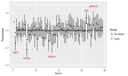
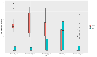
(a)	(b)
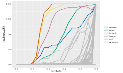
(c)	(d)

Figure 1: Analysis of the IBD microbiome data. (a) Lasso estimates, de-biased estimates and $95\%$ confidence intervals of the regression coefficients. Species selected based on the CIs are annotated. (b) Boxplots of log-relative abundances of the five identified species. The red and blue boxplots correspond to controls and cases samples respectively. (c) Fitted probability plot. (d) Selection stability plot.

Figure 1 (a) shows the Lasso estimates, de-biased estimates and $95\%$ confidence intervals of the regression coefficients in the model. Five bacteria were selected using our methods with the 95% CI not including zero, including Prevotella_copri, Ruminococcus_bromii, Clostridium_leptum, Escherichia_coli and Ruminococcus_gnavus. The estimated coefficients and the corresponding 95% CIs are summarized in Table 1. Among them, Prevotella_copri, Ruminococcus_bromii, Clostridium_leptum are negatively associated with the risk of IBD, indicating possible beneficial effects on IBD. On the other hand, Escherichia_coli and Ruminococcus_gnavus are positively associated with IBD. Figure 1 (b) plots the log-relative abundances of the five identified species in IBD children and in controls, indicating the the identified bacterial species indeed showed differential abundances between IBD cases and controls.

Our results confirm the results from other studies. Kaakoush et al. (2012) showed healthy people have high level of Prevotella_copri within their fecal microbial compared to Crohn’s disease patients. Ruminococcus_bromii and Clostridium_leptum (Mondot et al., 2011; Sokol et al., 2009; Kabeerdoss et al., 2013) were also shown to be negatively associated with the risk of IBD. Furthermore, Rhodes (2007) pointed out the association of an increase of Escherichia_coli and IBD. Matsuoka and Kanai (2015) also indicated the abundance of Ruminococcus_gnavus is higher in IBD patients.

Table 1: Selected bacteria and their corresponding phylum, estimated coefficients(standard errors in the parenthesis) and $95\%$ confidence intervals.

Bacteria name	Phylum	${\boldsymbol{\beta}}$(se)		CI
Prevotella_copri	Bacteroidetes	$-0$.	$15(0.042)$	$(-0.23,-0.064)$
Ruminococcus_bromii	Firmicutes	$-0$.	$22(0.043)$	$(-0.31,-0.18)$
Clostridium_leptum	Firmicutes	$-0$.	$15(0.052)$	$(-0.25,-0.048)$
Escherichia_coli	Proteobacteria	$0$.	$14(0.035)$	$(0.074,0.21)$
Ruminococcus_gnavus	Firmicutes	$0$.	$13(0.045)$	$(0.043,0.22)$

4.2 Stability, model fit and prediction evaluation

To assess how stable the results are, we performed stability selection analysis (Meinshausen and Bühlmann, 2010) by sample splitting. Among the 50 replications, each time we randomly sampled two third of the data including 56 cases and 16 controls and fit the model under different tuning parameters. Figure 1 (d) shows the selection probability for each of the bacteria versus values of the tuning parameter. We see that the selected species in the previous section have the highest stability selection probabilities, indicating the 5 species selected are very stable. Figure 1 (c) shows the fitted probability curve that is constructed based on the five identified species, indicating that our model fits the data well.

We then evaluate the performance of prediction based on the IBD data. The data was randomly separated into a training set of 56 cases and 16 controls that is used to estimate the parameters and a testing set of 28 cases and 8 controls that is used to evaluate the prediction performance. We used the estimated parameters to predict the IBD status in the testing set and evaluated the performance based on area under the ROC curve (AUCs). The procedure was repeated 50 times. The average AUC (se) are 0.92(0.049) , 0.93(0.043) and 0.93 (0.051) based on Lasso, debiased Lasso and de-biased Lasso using only the selected bacterial species, indicating that the model can predict IBD very well.

5 Simulation Studies

We evaluate the performance of of the proposed methods through a set of simulation studies. In order to simulate covariate $Z$ and outcome $Y$, we simulate the true bacterial abundances $W$, where each row of $W$ is generated from a log-normal distribution $\ln N(\mu,{\boldsymbol{\Sigma}})$, where ${\boldsymbol{\Sigma}}_{ij}=\zeta^{|i-j|}$ with $\zeta=0.2$ is the covariance matrix to reflect the correlation between different taxa. Mean parameters are set as $\mu_{j}=\frac{p}{2}$ for $j=1,\ldots,5$ and $\mu_{j}=1$ for $j=6,\ldots p$. The log-compositional covariate matrix $\mathbf{Z}$ is obtained by normalizing the true abundances

$$\mathbf{Z}_{ij}=\log\left(\frac{W_{ij}}{\sum_{k=1}^{p}W_{ik}}\right),$$

for $i=1,2,\ldots,n$ and $j=1,2,\ldots,p$. The true parameter ${\boldsymbol{\beta}}$ is

$${\boldsymbol{\beta}}=(0.45,-0.4,0.45,0,-0.5,0,0,0,0,0,-0.6,0,0.3,0,0,0.3,0,\ldots 0)$$

and ${\boldsymbol{\beta}}_{0}=-1$. Based on these covariates, we simulate the binary outcome $Y$ based on the logistic probability $p_{i}=\text{expit}(\mathbf{Z}_{i}^{\top}{\boldsymbol{\beta}}+{\boldsymbol{\beta}}_{0})$ and obtained the number of cases and controls at a 2:3 ratio. Different dimensions and sample sizes are considered and simulations are repeated 100 times for each setting. The true regression coefficients ${\boldsymbol{\beta}}$ are assumed to satisfy the following linear constraints:

$$\sum_{i=1}^{10}{\boldsymbol{\beta}}_{i}=0,\sum_{i=11}^{16}{\boldsymbol{\beta}}_{i}=0,\sum_{i=17}^{20}{\boldsymbol{\beta}}_{i}=0,\sum_{i=21}^{23}{\boldsymbol{\beta}}_{i}=0,$$

$$\sum_{i=24}^{30}{\boldsymbol{\beta}}_{i}=0,\sum_{i=31}^{32}{\boldsymbol{\beta}}_{i}=0,\sum_{i=33}^{40}{\boldsymbol{\beta}}_{i}=0,\sum_{i=41}^{p}{\boldsymbol{\beta}}_{i}=0.$$

5.1 Simulation results

We evaluate the performance of the simulation by comparing the coverage probability, length of the confidence interval and the true positive and false positive of selecting variables based on the confidence interval. We compare the results of fitting the models with no constraint, one constraint, true constraint and misspecified constraints specified below,

$$\sum_{i=1}^{4}{\boldsymbol{\beta}}_{i}=0,\sum_{i=5}^{12}{\boldsymbol{\beta}}_{i}=0,\sum_{i=13}^{23}{\boldsymbol{\beta}}_{i}=0,\sum_{i=24}^{30}{\boldsymbol{\beta}}_{i}=0,\sum_{i=31}^{p}{\boldsymbol{\beta}}_{i}=0.$$

Figure 2 shows that the coverage probabilities are closer to $95\%$ and the length of CIs decrease as sample size becomes larger. In addition, the coverage probabilities under true constraints are closer to the correct coverage probability ($95\%$) especially when $n$ is relatively larger($n=200,500$). As for length of CIs, the CIs using the true constraints have the shortest CIs while the length of the CIs for single constraint and no constraints are relatively wider. We did not compare the length of CI for using misspecified constraints because the coverage probability in this case is really poor. The figure also shows that the coverage probabilities are sensitive to the constraints when sample size becomes larger and the length is sensitive to the constraints for small sample size. This is expected as when the sample size is small, we are more likely to obtain wider CI, and using the correct constraints, which provide more information, would provide shorter CI. While for the coverage probability, since our algorithm provides an asymptotic CI, the sample size has bigger effects than the constraints. The coverage probability becomes really poor when the constraints are misspecified when $n=500$.

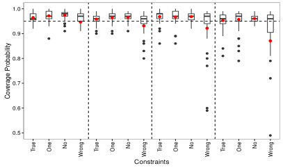
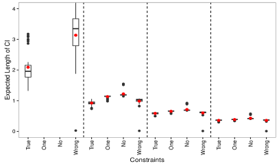
(a)	(b)
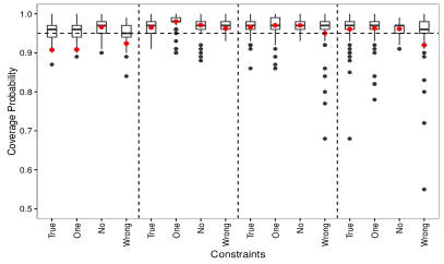
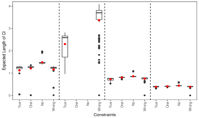
(c)	(d)

Figure 2: Coverage probabilities and length of confidence intervals based on 100 simulations for $p=50$ ((a) and (b)) and $p=100$ ((c) and (d)) and $n=50,100,200,500$ (separated by vertical dashed lines).

Table 2 shows the true positive and false positive rates of selecting the significant variables using the $95\%$ confidence interval under multiple, one, no and misspecified constraints for various dimensions $p$ and sample sizes $n$. The false positive rates are correctly controlled under $5\%$ for all models, even when the constraints are misspecified. However, models with correctly specified linear constraints have higher true positive rates. When the sample size is 500, true positive rate is greater than $90\%$, which is the highest among all models considered.

Table 2: True /False positive rates of the significant variables selected by the $95\%$ confidence interval using multiple, one, no and misspecified constraints. $p=50,100$ and $n=50,100,200,500$ are considered.

$n$		TP	FP		TP	FP		TP	FP		TP	FP
		Multi			One			No			Wrong
$p=50$
50		0.069	0.034		0.026	0.025		0.029	0.026		0.054	0.036
100		0.260	0.038		0.206	0.031		0.141	0.034		0.299	0.038
200		0.569	0.026		0.549	0.025		0.411	0.030		0.546	0.037
500		0.914	0.038		0.897	0.030		0.840	0.038		0.814	0.058
$p=100$
50		0.220	0.045		0.071	0.044		0.109	0.034		0.134	0.046
100		0.103	0.035		0.023	0.016		0.107	0.026		0.154	0.027
200		0.431	0.030		0.389	0.025		0.283	0.029		0.481	0.032
500		0.907	0.032		0.873	0.029		0.801	0.037		0.804	0.042

6 Discussion

We have considered estimation and inference for the generalized linear models with high dimensional compositional covariates. In order to accounting for the nature of compositional data, a group of linear constraints are imposed on the regression coefficients to ensure subcompositional coherence. With these constraints, the standard GLM Lasso algorithm based on Taylor expansion and coordinate descent algorithm does not work due to the non-separable nature of the penalty function. Instead, a generalized accelerated proximal gradient algorithm was developed to estimate the regression coefficients. To make statistical inference, a de-biased procedure is proposed to construct valid confidence intervals of the regression coefficients, which could be used for hypothesis testing as well as identifying species that are associated with the outcome. Application of the method to an analysis of IBD microbiome data has identified five bacterial species that are associated with pediatric IBD with a high stability. The identified model has also shown a great prediction performance based on cross-validation.

The approach we took in deriving the confidence intervals follows that of Javanmard and Montanari (2014) by first obtaining an debiased estimates of the regression coefficients. Alternatively, one can consider the approach based on post-selection inference for $\ell_{1}$-penalized likelihood models (Taylor and Tibshirani, 2017). However, one needs to modify the methods for Taylor and Tibshirani (2017) to take into account the linear constraints of the regression coefficients. It would be interesting to compare the performance of this alternative approach.

Appendix

We provide proofs for the main theorems in the paper.

Lemma 6.1

If Conditions C1 and C2 hold, then for any matrix $A$,

$$|(\mathbf{I}_{p}-P_{C})A|_{\infty}\leq k_{0}|A|_{\infty}.$$

The proof for this lemma is in the appendix of Shi et al. (2016).

Proof of Theorem 3.1

Proof 6.2

By the definition of $\hat{{\boldsymbol{\beta}}}^{n}$ and (4), we have:

$$-\dfrac{1}{n}[Y^{\top}\widetilde{\mathbf{Z}}\hat{{\boldsymbol{\beta}}}^{n}-\sum_{i=1}^{n}A(\widetilde{Z}_{i}^{\top}\hat{{\boldsymbol{\beta}}}^{n})]+\lambda||\hat{{\boldsymbol{\beta}}}^{n}||_{1}\leq-\dfrac{1}{n}[Y^{\top}\widetilde{\mathbf{Z}}{\boldsymbol{\beta}}-\sum_{i=1}^{n}A(\widetilde{Z}_{i}^{\top}{\boldsymbol{\beta}})]+\lambda||{\boldsymbol{\beta}}||_{1}.$$ (11)

Denote $h=\hat{{\boldsymbol{\beta}}}^{n}-{\boldsymbol{\beta}}$, and $S_{h}$ be the set of index of the $s$ largest absolute values of $h$. Then rearrange (11), we get:

$$\lambda(\|{\boldsymbol{\beta}}\|_{1}-\|\hat{{\boldsymbol{\beta}}}^{n}\|_{1})\geq-\dfrac{1}{n}[Y^{\top}\widetilde{\mathbf{Z}}h-\sum_{i=1}^{n}(A(\widetilde{Z}_{i}^{\top}\hat{{\boldsymbol{\beta}}}^{n})-A(\widetilde{Z}_{i}^{\top}{\boldsymbol{\beta}}))].$$ (12)

Notice that,

$$\|{\boldsymbol{\beta}}\|_{1}-\|\hat{{\boldsymbol{\beta}}}^{n}\|_{1}= \|{\boldsymbol{\beta}}_{supp({\boldsymbol{\beta}})}\|_{1}-\|\hat{{\boldsymbol{\beta}}}_{supp({\boldsymbol{\beta}})}^{n}\|_{1}-\|\hat{{\boldsymbol{\beta}}}_{supp({\boldsymbol{\beta}})^{c}}^{n}\|_{1},$$

$$\leq \|{\boldsymbol{\beta}}_{supp({\boldsymbol{\beta}})}-\hat{{\boldsymbol{\beta}}}_{supp({\boldsymbol{\beta}})}^{n}\|_{1}-\|h_{supp({\boldsymbol{\beta}})^{c}}\|_{1},$$

$$\leq \|h_{S_{h}}\|_{1}-\|h_{S^{c}_{h}}\|_{1}.$$ (13)

Furthermore, for each $i$ applied the mean value theorem to $A$ defined in 2, there exists $\widetilde{\beta_{i}}^{0}$ such that $A(\widetilde{Z}_{i}^{\top}\hat{\beta}^{n})-A(\widetilde{Z}_{i}^{\top}\beta)=\mu(\widetilde{\beta},\widetilde{Z}_{i})\widetilde{Z}_{i}^{\top}h+\dfrac{1}{2}v(\widetilde{\beta_{i}}^{0},\widetilde{Z}_{i})\left(\widetilde{Z}_{i}^{\top}h\right)^{2}$. Then we have:

$$-\dfrac{1}{n}[Y^{\top}\widetilde{\mathbf{Z}}h-\sum_{i=1}^{n}(A(\widetilde{Z}_{i}^{\top}\hat{\beta}^{n})-A(\widetilde{Z}_{i}^{\top}\beta))]$$ (14)

$$\geq-\dfrac{1}{n}[Y^{\top}\widetilde{\mathbf{Z}}h-\mu(\beta,\widetilde{\mathbf{Z}})^{\top}\widetilde{\mathbf{Z}}h)],$$

$$\geq-\dfrac{1}{n}(Y-\mu(\beta,\widetilde{\mathbf{Z}}))^{\top}\widetilde{\mathbf{Z}}h,$$

$$\geq-\dfrac{1}{n}\|Y-\mu(\beta,\widetilde{\mathbf{Z}})^{\top}\widetilde{\mathbf{Z}}\|_{\infty}\cdot\|h\|_{1}=-\dfrac{1}{n}\|(Y-\mu(\beta,\widetilde{\mathbf{Z}}))^{\top}\widetilde{\mathbf{Z}}\|_{\infty}\cdot(\|h_{S_{h}}\|_{1}+\|h_{S^{c}_{h}}\|_{1}).$$

When the event $\|(Y-\mu(\beta,\widetilde{\mathbf{Z}}))^{\top}\widetilde{\mathbf{Z}}\|_{\infty}\leq\dfrac{n\lambda}{\tau}$ holds, we have:

$$\lambda(\|{\boldsymbol{\beta}}\|_{1}-\|\hat{{\boldsymbol{\beta}}}^{n}\|_{1})\geq-\dfrac{1}{n}\cdot\frac{n\lambda}{\tau}\cdot(\|h_{S_{h}}\|_{1}+\|h_{S^{c}_{h}}\|_{1}).$$ (15)

So by (12), (6.2) and (15) we have:

$$\lambda(\|h_{S_{h}}\|_{1}-\|h_{S^{c}_{h}}\|_{1})\geq\lambda(\|{\boldsymbol{\beta}}\|_{1}-\|\hat{{\boldsymbol{\beta}}}^{n}\|_{1})\geq-\frac{\lambda}{\tau}\cdot(\|h_{S_{h}}\|_{1}+\|h_{S^{c}_{h}}\|_{1}).$$

That is,

$$\|h_{S^{c}_{h}}\|_{1}\leq\dfrac{\tau+1}{\tau-1}\|h_{S_{h}}\|_{1}.$$ (16)

Then by the KKT condition of optimization problem (4), we have:

$$\|\widetilde{\mathbf{Z}}^{\top}(Y-\mu(\hat{{\boldsymbol{\beta}}}^{n},\widetilde{\mathbf{Z}}))+C\bm{\eta}\|_{\infty}\leq n\lambda,$$ (17)

for some $\bm{\eta}\in{\mathbb{R}}^{r}$. Then by Lemma 1,

$$\|(\mathbf{I}_{p}-P_{C})\left(\widetilde{\mathbf{Z}}^{\top}(Y-\mu(\hat{{\boldsymbol{\beta}}}^{n},\widetilde{\mathbf{Z}}))+C\bm{\mu}\right)\|_{\infty} \leq k_{0}\|\widetilde{\mathbf{Z}}^{\top}(Y-\mu(\hat{{\boldsymbol{\beta}}}^{n},\widetilde{\mathbf{Z}}))+C\bm{\mu}\|_{\infty}\leq k_{0}n\lambda.$$ (18)

Then as

$$(\mathbf{I}_{p}-P_{C})(\widetilde{\mathbf{Z}}^{\top}(Y-\mu(\hat{{\boldsymbol{\beta}}}^{n},\widetilde{\mathbf{Z}}))+C\bm{\mu}) =(\mathbf{I}_{p}-P_{C})\widetilde{\mathbf{Z}}^{\top}(Y-\mu(\hat{{\boldsymbol{\beta}}}^{n},\widetilde{\mathbf{Z}}))+(\mathbf{I}_{p}-P_{C})C\bm{\mu},$$

$$=\widetilde{\mathbf{Z}}^{\top}(Y-\mu(\hat{{\boldsymbol{\beta}}}^{n},\widetilde{\mathbf{Z}})).$$

with the the assumption that $\|(Y-\mu({\boldsymbol{\beta}},\widetilde{\mathbf{Z}}))^{\top}\widetilde{\mathbf{Z}}\|_{\infty}\leq\dfrac{n\lambda}{\tau}$, we have:

$$\|\widetilde{\mathbf{Z}}^{\top}(\mu(\hat{{\boldsymbol{\beta}}}^{n},\widetilde{\mathbf{Z}})-\mu({\boldsymbol{\beta}},\widetilde{\mathbf{Z}}))\| \leq\|\widetilde{\mathbf{Z}}^{\top}(Y-\mu(\hat{{\boldsymbol{\beta}}}^{n},\widetilde{\mathbf{Z}}))\|_{\infty}+\|\widetilde{\mathbf{Z}}^{\top}(Y-\mu({\boldsymbol{\beta}},\widetilde{\mathbf{Z}}))\|_{\infty}\leq k_{0}n\lambda+\dfrac{n\lambda}{\tau}.$$

As $\|\widetilde{\mathbf{Z}}^{\top}(\mu(\hat{{\boldsymbol{\beta}}}^{n},\widetilde{\mathbf{Z}})-\mu({\boldsymbol{\beta}},\widetilde{\mathbf{Z}}))\|=\|\widetilde{\mathbf{Z}}^{\top}\mathbf{V}({\boldsymbol{\beta}}^{0},\widetilde{\mathbf{Z}})\widetilde{\mathbf{Z}}h\|_{\infty}$, we get

$$\|\widetilde{\mathbf{Z}}^{\top}\mathbf{V}({\boldsymbol{\beta}}^{0},\widetilde{\mathbf{Z}})\widetilde{\mathbf{Z}}h\|_{\infty}\leq k_{0}n\lambda+\dfrac{n\lambda}{\tau}.$$

Since $\mathbf{V}({\boldsymbol{\beta}}^{0},\widetilde{\mathbf{Z}})$ is a diagonal matrix with all its nonzero elements greater than zero, define $\widetilde{\mathbf{Z}}_{v}=\mathbf{V}^{\frac{1}{2}}({\boldsymbol{\beta}}^{0},\widetilde{\mathbf{Z}})\widetilde{\mathbf{Z}}$, where $\mathbf{V}^{\frac{1}{2}}({\boldsymbol{\beta}}^{0},\widetilde{\mathbf{Z}})={\rm diag}\{(v({\boldsymbol{\beta}}^{0},Z_{1}))^{\frac{1}{2}},\dots,(v({\boldsymbol{\beta}}^{0},Z_{n}))^{\frac{1}{2}}\}$. So $\widetilde{\mathbf{Z}}_{v}^{\top}\widetilde{\mathbf{Z}}_{v}=\widetilde{\mathbf{Z}}^{\top}\mathbf{V}({\boldsymbol{\beta}}^{0},\widetilde{\mathbf{Z}})\widetilde{\mathbf{Z}}$. Using Lemma 5.1 in Cai and Zhang (2013), we have:

$$|\langle\widetilde{\mathbf{Z}}_{v}h_{S_{h}},\widetilde{\mathbf{Z}}_{v}h_{S^{c}_{h}}\rangle| \leq\theta_{s,s}(\widetilde{\mathbf{Z}}_{v})\|h_{S_{h}}\|_{2}\cdot\max(\|h_{S^{c}_{h}}\|_{\infty},\|h_{S^{c}_{h}}\|_{1}/s)\sqrt{s},$$

$$\leq\sqrt{s}\theta_{s,s}(\widetilde{\mathbf{Z}}_{v})\|h_{S_{h}}\|_{2}\cdot\frac{\tau+1}{\tau-1}\|h_{S_{h}}\|_{1}/s,$$

$$\leq\dfrac{\tau+1}{\tau-1}\theta_{s,s}(\widetilde{\mathbf{Z}}_{v})\|h_{S_{h}}\|^{2}_{2}.$$

Then,

$$(k_{0}n\lambda+\dfrac{n\lambda}{\tau})\|h_{S_{h}}\|_{1} \geq\|\widetilde{\mathbf{Z}}^{\top}\mathbf{V}({\boldsymbol{\beta}}^{0},\widetilde{\mathbf{Z}})\widetilde{\mathbf{Z}}h\|_{\infty}\|h_{S_{h}}\|_{1}\geq\langle\widetilde{\mathbf{Z}}_{v}^{\top}\widetilde{\mathbf{Z}}_{v}h,h_{S_{h}}\rangle,$$

$$=\langle\widetilde{\mathbf{Z}}_{v}h_{S_{h}},\widetilde{\mathbf{Z}}_{v}h_{S_{h}}\rangle+\langle\widetilde{\mathbf{Z}}_{v}h_{S_{h}},\widetilde{\mathbf{Z}}_{v}h_{S^{c}_{h}}\rangle,$$

$$\geq\|\widetilde{\mathbf{Z}}_{v}h_{S_{h}}\|_{2}^{2}-\dfrac{\tau+1}{\tau-1}\theta_{s,s}(\widetilde{\mathbf{Z}}_{v})\|h_{S_{h}}\|^{2}_{2},$$

$$\geq\left(\delta_{2s}^{-}(\widetilde{\mathbf{Z}}_{v})-\dfrac{\tau+1}{\tau-1}\theta_{s,s}(\widetilde{\mathbf{Z}}_{v})\right)\|h_{S_{h}}\|^{2}_{2},$$

$$\geq\left(\dfrac{3\tau-1}{2(\tau-1)}\delta_{2s}^{-}(\widetilde{\mathbf{Z}}_{v})-\dfrac{\tau+1}{2(\tau-1)}\delta_{2s}^{+}(\widetilde{\mathbf{Z}}_{v})\right)\|h_{S_{h}}\|^{2}_{1}/s.$$ (19)

So from (6.2) we have:

$$\|h_{S_{h}}\|_{1} \leq\dfrac{s\left(k_{0}n\lambda+\dfrac{n\lambda}{\tau}\right)}{\left(\dfrac{3\tau-1}{2(\tau-1)}\delta_{2s}^{-}(\widetilde{\mathbf{Z}}_{v})-\dfrac{\tau+1}{2(\tau-1)}\delta_{2s}^{+}(\widetilde{\mathbf{Z}}_{v})\right)},$$

$$\leq s\dfrac{k_{0}n\lambda+\dfrac{n\lambda}{\tau}}{2n\tau\phi_{0}/(\tau-1)}.$$ (20)

So combine (16) and (6.2), we have:

$$\|\hat{{\boldsymbol{\beta}}}^{n}-{\boldsymbol{\beta}}\|_{1}=\|h_{S_{h}}\|_{1}+\|h_{S^{c}_{h}}\|_{1}\leq\dfrac{2\tau}{\tau-1}\|h_{S_{h}}\|_{1}\leq\dfrac{s\lambda(k_{0}+1/\tau)}{\phi_{0}}.$$

Take $\lambda=\tau\tilde{c}\sqrt{(\log p)/n}$, so we have:

$${\mathbb{P}}\left(\|\hat{\beta}^{n}-\beta\|_{1}\leq\dfrac{s\lambda(k_{0}+1/\tau)}{\phi_{0}}\right) \geq 1-{\mathbb{P}}\left(\|(Y-\mu(\beta,\widetilde{\mathbf{Z}}))^{\top}\widetilde{\mathbf{Z}}\|_{\infty}>\dfrac{n\lambda}{\tau}\right)$$

$$\geq 1-\sum_{i=1}^{p}{\mathbb{P}}\left(|((Y-\mu(\beta,\widetilde{\mathbf{Z}}))^{\top}\widetilde{\mathbf{Z}})_{i}|>\dfrac{n\lambda}{\tau}\right)$$

$$\geq 1-2\sum_{i=1}^{p}\exp\left(-\dfrac{(\sqrt{n}\lambda/\tau}{2K^{2}}\right)\geq 1-2p^{1-\tilde{c}^{2}/(2K^{2})}$$

Proof of Lemma 3.2

Proof 6.3

We first provide a bound for ${\boldsymbol{\Sigma}}$. Notice that:

$$\bm{\Omega}_{{\boldsymbol{\beta}}}{\boldsymbol{\Sigma}}-(\mathbf{I}_{p}-P_{C}) =\dfrac{1}{n}\sum_{k=1}^{n}\left(\bm{\Omega}_{{\boldsymbol{\beta}}}v({\boldsymbol{\beta}},\widetilde{Z}_{k})\widetilde{Z}_{k}\widetilde{Z}_{k}^{\top}-(\mathbf{I}_{p}-P_{C})\right),$$

$$=\dfrac{1}{n}\sum_{k=1}^{n}\left(\bm{\Omega}_{{\boldsymbol{\beta}}}^{1/2}\bm{\Omega}_{{\boldsymbol{\beta}}}^{1/2}v({\boldsymbol{\beta}},\widetilde{Z}_{k})\widetilde{Z}_{k}\widetilde{Z}_{k}^{\top}\bm{\Omega}^{1/2}_{{\boldsymbol{\beta}}}{\boldsymbol{\Sigma}}_{{\boldsymbol{\beta}}}^{1/2}-(\mathbf{I}_{p}-P_{C})\right).$$

The last equality is true as ${\boldsymbol{\Sigma}}_{{\boldsymbol{\beta}}}^{1/2}\bm{\Omega}^{1/2}_{{\boldsymbol{\beta}}}\widetilde{Z}_{k}=(\mathbf{I}_{p}-P_{C})\widetilde{Z}_{k}=\widetilde{Z}_{k}$ for $k=1,2\ldots,n$. Then notice that ${\mathbb{E}}\bm{\Omega}_{{\boldsymbol{\beta}}}v({\boldsymbol{\beta}},\widetilde{Z}_{k})\widetilde{Z}_{k}\widetilde{Z}_{k}^{\top}={\mathbb{E}}\bm{\Omega}_{{\boldsymbol{\beta}}}{\boldsymbol{\Sigma}}_{{\boldsymbol{\beta}}}=\mathbf{I}_{p}-P_{C}$, so define:

$$v_{k}^{(ij)}=\bm{\Omega}_{i,\cdot}^{1/2}\bm{\Omega}_{{\boldsymbol{\beta}}}^{1/2}v({\boldsymbol{\beta}},\widetilde{Z}_{k})\widetilde{Z}_{k}\widetilde{Z}_{k}^{\top}\bm{\Omega}^{1/2}_{{\boldsymbol{\beta}}}({\boldsymbol{\Sigma}}_{{\boldsymbol{\beta}}})_{\cdot,j}^{1/2}-(\mathbf{I}_{p}-P_{C})_{i,j},$$

we know that ${\mathbb{E}}v_{k}^{(ij)}=0$ for $k=1,2\ldots,n$ and any $i,j$. Then by the proof of Lemma 6.2 in Javanmard and Montanari (2014), we have:

$$\|v_{k}^{(ij)}\|_{\psi_{1}} \leq 2\|\bm{\Omega}_{i,\cdot}^{1/2}\bm{\Omega}_{{\boldsymbol{\beta}}}^{1/2}v({\boldsymbol{\beta}},\widetilde{Z}_{k})\widetilde{Z}_{k}\widetilde{Z}_{k}^{\top}\bm{\Omega}^{1/2}_{{\boldsymbol{\beta}}}({\boldsymbol{\Sigma}}_{{\boldsymbol{\beta}}})_{\cdot,j}^{1/2}\|_{\psi_{1}},$$

$$\leq 2v({\boldsymbol{\beta}},\widetilde{Z}_{k})\|\bm{\Omega}_{i,\cdot}^{1/2}\bm{\Omega}_{{\boldsymbol{\beta}}}^{1/2}\widetilde{Z}_{k}\|_{\psi_{2}}\|({\boldsymbol{\Sigma}}_{{\boldsymbol{\beta}}})_{\cdot,j}\bm{\Omega}^{1/2}_{{\boldsymbol{\beta}}}\widetilde{Z}_{k}\|_{\psi_{2}},$$

$$\leq 2\|({\boldsymbol{\Sigma}}_{{\boldsymbol{\beta}}})_{\cdot,j}\|_{2}\|\bm{\Omega}_{i,\cdot}^{1/2}\|_{2}\cdot\|\bm{\Omega}_{{\boldsymbol{\beta}}}^{1/2}\widetilde{Z}_{k}\|_{\psi_{2}}\|\bm{\Omega}^{1/2}_{{\boldsymbol{\beta}}}\widetilde{Z}_{k}\|_{\psi_{2}},$$

$$\leq 2\sqrt{C_{\text{max}}/C_{\text{min}}}\kappa^{2}\equiv\kappa_{1}^{\prime}.$$

Then by inequality for centered sub-exponential random variables from Bühlmann and Van De Geer (2011), we have:

$${\mathbb{P}}\left(\dfrac{1}{n}|\sum_{k=1}^{n}v_{k}^{(ij)}|\geq\gamma\right)\leq\exp\left(-\dfrac{n}{6}\min\left\{\left(\dfrac{\gamma}{e\kappa^{{}^{\prime}}}\right)^{2},\left(\dfrac{\gamma}{e\kappa^{{}^{\prime}}}\right)\right\}\right).$$

Pick $\gamma=c\sqrt{(\log p)/n}$ with $c\leq e\kappa_{1}^{\prime}\sqrt{n/(\log p)}$, we have:

$${\mathbb{P}}\left(\dfrac{1}{n}|\sum_{k=1}^{n}v_{k}^{(ij)}|\geq c\sqrt{\dfrac{\log p}{n}}\right)\leq 2p^{-c^{2}/(6e^{2}\kappa_{1}^{\prime 2})}=2p^{-c^{2}C_{\text{min}}/(24e^{2}C_{\text{max}}\kappa^{4})}.$$ (21)

Since (21) is true for all $i,j$, we have:

$${\mathbb{P}}\left(|\bm{\Omega}_{{\boldsymbol{\beta}}}{\boldsymbol{\Sigma}}-(\mathbf{I}_{p}-P_{C})|_{\infty}\geq c\sqrt{(\log p)/n}\right)\leq 2p^{-c^{2}C_{\text{min}}/(24e^{2}C_{\text{max}}\kappa^{4})+2}=2p^{-c_{1}^{{}^{\prime\prime}}}.$$

Then by the following inequality:

$${\mathbb{P}}\left(|\bm{\Omega}_{{\boldsymbol{\beta}}}\widehat{{\boldsymbol{\Sigma}}}-(\mathbf{I}_{p}-P_{C})|_{\infty}\geq c\sqrt{(\log p)/n}\right)$$

$$\leq{\mathbb{P}}\left(|\bm{\Omega}_{{\boldsymbol{\beta}}}{\boldsymbol{\Sigma}}-(\mathbf{I}_{p}-P_{C})|_{\infty}+|\bm{\Omega}_{{\boldsymbol{\beta}}}({\boldsymbol{\Sigma}}-\widehat{{\boldsymbol{\Sigma}}})|\geq c\sqrt{(\log p)/n}\right)$$

$$\leq{\mathbb{P}}\left(|\bm{\Omega}_{{\boldsymbol{\beta}}}{\boldsymbol{\Sigma}}-(\mathbf{I}_{p}-P_{C})|_{\infty}\geq c\sqrt{(\log p)/n}\right)+{\mathbb{P}}\left(|\bm{\Omega}_{{\boldsymbol{\beta}}}({\boldsymbol{\Sigma}}-\widehat{{\boldsymbol{\Sigma}}})|\geq c\sqrt{(\log p)/n}\right)$$

Notice that:

$$\left|\bm{\Omega}_{{\boldsymbol{\beta}}}({\boldsymbol{\Sigma}}-\widehat{{\boldsymbol{\Sigma}}})\right|_{\infty} =\frac{1}{n}\left|\sum_{k=1}^{n}\left(\bm{\Omega}_{{\boldsymbol{\beta}}}\left(v({\boldsymbol{\beta}},\widetilde{Z}_{k})-v(\hat{{\boldsymbol{\beta}}}^{n},\widetilde{Z}_{k})\right)\widetilde{Z}_{k}\widetilde{Z}_{k}^{\top}\right)\right|_{\infty}$$

$$\leq\frac{1}{n}\left|\sum_{k=1}^{n}\left(C\|\hat{{\boldsymbol{\beta}}}^{n}-{\boldsymbol{\beta}}\|_{1}\bm{\Omega}_{{\boldsymbol{\beta}}}\widetilde{Z}_{k}\widetilde{Z}_{k}^{\top}\right)\right|_{\infty}$$

As

$$\frac{1}{n}\sum_{k=1}^{n}\left(\bm{\Omega}_{{\boldsymbol{\beta}}}\widetilde{Z}_{k}\widetilde{Z}_{k}^{\top}\right)\rightarrow{\mathbb{E}}\bm{\Omega}_{{\boldsymbol{\beta}}}\widetilde{Z}_{1}\widetilde{Z}_{1}^{\top}={\mathbb{E}}\bm{\Omega}_{{\boldsymbol{\beta}}}\Theta,$$

together with the result we obtain from theorem 3.1,

$${\mathbb{P}}\left(|\bm{\Omega}_{{\boldsymbol{\beta}}}({\boldsymbol{\Sigma}}-\widehat{{\boldsymbol{\Sigma}}})|_{\infty}\geq c\sqrt{(\log p)/n}\right) \leq{\mathbb{P}}\left(\frac{1}{n}\left|\sum_{k=1}^{n}\left(C\|\hat{{\boldsymbol{\beta}}}^{n}-{\boldsymbol{\beta}}\|_{1}\bm{\Omega}_{{\boldsymbol{\beta}}}\widetilde{Z}_{k}\widetilde{Z}_{k}^{\top}\right)\right|_{\infty}\geq c\sqrt{(\log p)/n}\right)$$

$$\leq 2p^{1-\hat{c}^{2}/(2K^{2})}=2p^{-c_{2}^{{}^{\prime\prime}}}$$

where $\hat{c}=\frac{c\phi_{0}}{C|\bm{\Omega}_{{\boldsymbol{\beta}}}\Theta|_{\infty}s(k_{0}\tau+1)}$. So finally:

$${\mathbb{P}}\left(|\bm{\Omega}_{{\boldsymbol{\beta}}}\widehat{{\boldsymbol{\Sigma}}}-(\mathbf{I}_{p}-P_{C})|_{\infty}\geq c\sqrt{(\log p)/n}\right)$$

$$\leq{\mathbb{P}}\left(|\bm{\Omega}_{{\boldsymbol{\beta}}}{\boldsymbol{\Sigma}}-(\mathbf{I}_{p}-P_{C})|_{\infty}\geq c\sqrt{(\log p)/n}\right)+{\mathbb{P}}\left(|\bm{\Omega}_{{\boldsymbol{\beta}}}({\boldsymbol{\Sigma}}-\widehat{{\boldsymbol{\Sigma}}})|_{\infty}\geq c\sqrt{(\log p)/n}\right)$$

$$\leq 2p^{-c_{1}^{{}^{\prime\prime}}}+2p^{-c_{2}^{{}^{\prime\prime}}}$$

Proof of Theorem 3.3

Proof 6.4

As we obtained in lemma 3.2, $\Omega_{{\boldsymbol{\beta}}}$ is in the feasible set with a large probability. That is, event $|M\widehat{{\boldsymbol{\Sigma}}}-(\mathbf{I}_{p}-P_{C})|_{\infty}\geq c\sqrt{(\log p)/n}$ happens with large probability. Further more,

$${\mathbb{P}}\left(|(\mathbf{I}_{p}-P_{C})-M\widehat{{\boldsymbol{\Sigma}}}^{0}|_{\infty}\geq c\sqrt{(\log p)/n}\right) \leq{\mathbb{P}}\left(|M\widehat{{\boldsymbol{\Sigma}}}-(\mathbf{I}_{p}-P_{C})|_{\infty}\geq c\sqrt{(\log p)/n}\right)$$

$$+{\mathbb{P}}\left(|M(\widehat{{\boldsymbol{\Sigma}}}^{0}-\widehat{{\boldsymbol{\Sigma}}})|_{\infty}\geq c\sqrt{(\log p)/n}\right).$$

The bound for the first term on the RHS is the result from lemma 3.2. Applying the similar method to the second term, notice that $\|\hat{{\boldsymbol{\beta}}}^{0}-{\boldsymbol{\beta}}\|_{1}\leq\|\hat{{\boldsymbol{\beta}}}^{n}-{\boldsymbol{\beta}}\|_{1}$, hence, ${\mathbb{P}}(|M(\widehat{{\boldsymbol{\Sigma}}}^{0}-\widehat{{\boldsymbol{\Sigma}}})|_{\infty}\geq\allowbreak c\sqrt{(\log p)/n})\leq 4p^{-c_{2}^{{}^{\prime\prime}}}$. So,

$${\mathbb{P}}\left(|(\mathbf{I}_{p}-P_{C})-M\widehat{{\boldsymbol{\Sigma}}}^{0}|_{\infty}\geq c\sqrt{(\log p)/n}\right)\leq 2p^{-c_{1}^{{}^{\prime\prime}}}+6p^{-c_{2}^{{}^{\prime\prime}}}$$

Finally,

$$\|\Delta\|_{\infty} \leq\sqrt{n}\left|(\mathbf{I}_{p}-P_{C})-\widetilde{M}\widehat{{\boldsymbol{\Sigma}}}^{0}\right|_{\infty}\|\hat{{\boldsymbol{\beta}}}^{n}-{\boldsymbol{\beta}}\|_{1}$$

$$=\sqrt{n}\left|(\mathbf{I}_{p}-P_{C})\left((\mathbf{I}_{p}-P_{C})-\widetilde{M}\widehat{{\boldsymbol{\Sigma}}}^{0}\right)\right|_{\infty}\|\hat{{\boldsymbol{\beta}}}^{n}-{\boldsymbol{\beta}}\|_{1}$$

$$\leq k_{0}\sqrt{n}|(\mathbf{I}_{p}-P_{C})-M\widehat{{\boldsymbol{\Sigma}}}^{0}|_{\infty}\|\hat{{\boldsymbol{\beta}}}^{n}-{\boldsymbol{\beta}}\|_{1}$$

We have:

$${\mathbb{P}}\left(\|\Delta\|_{\infty}>\dfrac{c\tilde{c}k_{0}(k_{0}\tau+1)}{\phi_{0}}\cdot\dfrac{s\log p}{\sqrt{n}}\right)$$

$$\leq{\mathbb{P}}\left(\|\hat{{\boldsymbol{\beta}}}^{n}-{\boldsymbol{\beta}}\|_{1}\geq\dfrac{s\lambda(k_{0}+1/\tau)}{\phi_{0}}=\dfrac{s\tilde{c}(k_{0}\tau+1)\sqrt{(\log p)/n}}{\phi_{0}}\right)$$

$$+{\mathbb{P}}\left(|(\mathbf{I}_{p}-P_{C})-M\widehat{{\boldsymbol{\Sigma}}}^{0}|_{\infty}\geq\gamma=c\sqrt{(\log p)/n}\right)$$

$$\leq 2p^{-c^{\prime}}+2p^{-c_{1}^{{}^{\prime\prime}}}+6p^{-c_{2}^{{}^{\prime\prime}}}$$

So we have finished the proof.

References

• Aitchison (1982) Aitchison, J. (1982). The statistical analysis of compositional data. Journal of the Royal Statistical Society. Series B (Methodological) pages 139–177.
• Aitchison and Bacon-shone (1984) Aitchison, J. and Bacon-shone, J. (1984). Log contrast models for experiments with mixtures. Biometrika 71, 323–330.
• Bühlmann and Van De Geer (2011) Bühlmann, P. and Van De Geer, S. (2011). Statistics for high-dimensional data: methods, theory and applications. Springer Science & Business Media.
• Cai and Zhang (2013) Cai, T. T. and Zhang, A. (2013). Compressed sensing and affine rank minimization under restricted isometry. Signal Processing, IEEE Transactions on 61, 3279–3290.
• Cao et al. (2017) Cao, Y., Lin, W., and Li, H. (2017). Two-sample tests of high dimensional means for compositional data. Biometrika in press,.
• Chen and Chen (2008) Chen, J. and Chen, Z. (2008). Extended bayesian information criteria for model selection with large model spaces. Biometrika 95, 759–771.
• Javanmard and Montanari (2014) Javanmard, A. and Montanari, A. (2014). Confidence intervals and hypothesis testing for high-dimensional regression. The Journal of Machine Learning Research 15, 2869–2909.
• Kaakoush et al. (2012) Kaakoush, N. O., Day, A. S., Huinao, K. D., Leach, S. T., Lemberg, D. A., Dowd, S. E., and Mitchell, H. M. (2012). Microbial dysbiosis in pediatric patients with crohn’s disease. Journal of clinical microbiology 50, 3258–3266.
• Kabeerdoss et al. (2013) Kabeerdoss, J., Sankaran, V., Pugazhendhi, S., and Ramakrishna, B. S. (2013). Clostridium leptum group bacteria abundance and diversity in the fecal microbiota of patients with inflammatory bowel disease: a case–control study in india. BMC gastroenterology 13, 20.
• Kurtz et al. (2015) Kurtz, Z. D., Müller, C. L., Miraldi, E. R., Littman, D. R., Blaser, M. J., and Bonneau, R. A. (2015). Sparse and compositionally robust inference of microbial ecological networks. PLoS Comput Biol 11, e1004226.
• Lewis et al. (2015) Lewis, J. D., Chen, E. Z., Baldassano, R. N., Otley, A. R., Griffiths, A. M., Lee, D., Bittinger, K., Bailey, A., Friedman, E. S., Hoffmann, C., et al. (2015). Inflammation, antibiotics, and diet as environmental stressors of the gut microbiome in pediatric crohn’s disease. Cell host & microbe 18, 489–500.
• Lin et al. (2014) Lin, W., Shi, P., Feng, R., and Li, H. (2014). Variable selection in regression with compositional covariates. Biometrika page asu031.
• Matsuoka and Kanai (2015) Matsuoka, K. and Kanai, T. (2015). The gut microbiota and inflammatory bowel disease. In Seminars in immunopathology, volume 37, pages 47–55. Springer.
• Meinshausen and Bühlmann (2010) Meinshausen, N. and Bühlmann, P. (2010). Stability selection. Journal of the Royal Statistical Society: Series B (Statistical Methodology) 72, 417–473.
• Mondot et al. (2011) Mondot, S., Kang, S., Furet, J.-P., Aguirre de Cárcer, D., McSweeney, C., Morrison, M., Marteau, P., Dore, J., and Leclerc, M. (2011). Highlighting new phylogenetic specificities of crohn’s disease microbiota. Inflammatory bowel diseases 17, 185–192.
• Nesterov (2013) Nesterov, Y. (2013). Introductory lectures on convex optimization: A basic course, volume 87. Springer Science & Business Media.
• Ning et al. (2017) Ning, Y., Liu, H., et al. (2017). A general theory of hypothesis tests and confidence regions for sparse high dimensional models. The Annals of Statistics 45, 158–195.
• Rhodes (2007) Rhodes, J. M. (2007). The role of escherichia coli in inflammatory bowel disease. Gut 56, 610–612.
• Shi et al. (2016) Shi, P., Zhang, A., and Li, H. (2016). Regression analysis for microbiome compositional data. Ann. Appl. Stat. 10, 1019–1040.
• Sokol et al. (2009) Sokol, H., Seksik, P., Furet, J., Firmesse, O., Nion-Larmurier, I., Beaugerie, L., Cosnes, J., Corthier, G., Marteau, P., and Doré, J. (2009). Low counts of faecalibacterium prausnitzii in colitis microbiota. Inflammatory bowel diseases 15, 1183–1189.
• Su et al. (2014) Su, W., Boyd, S., and Candes, E. (2014). A differential equation for modeling nesterov’s accelerated gradient method: theory and insights. In Advances in Neural Information Processing Systems, pages 2510–2518.
• Taylor and Tibshirani (2017) Taylor, J. and Tibshirani, R. (2017). Post-selection inference for $\ell_{1}$-penalized likelihood models. https://arxiv.org/pdf/1602.07358.pdf in press,.
• Van de Geer et al. (2014) Van de Geer, S., Bühlmann, P., Ritov, Y., Dezeure, R., et al. (2014). On asymptotically optimal confidence regions and tests for high-dimensional models. The Annals of Statistics 42, 1166–1202.
• Zhang and Zhang (2014) Zhang, C.-H. and Zhang, S. S. (2014). Confidence intervals for low dimensional parameters in high dimensional linear models. Journal of the Royal Statistical Society: Series B (Statistical Methodology) 76, 217–242.