Choreographies in the Discrete Nonlinear Schrödinger Equations

Abstract

We study periodic solutions of the discrete nonlinear Schrödinger equation (DNLSE) that bifurcate from a symmetric polygonal relative equilibrium containing $n$ sites. With specialized numerical continuation techniques and a varying physically relevant parameter we can locate interesting orbits, including infinitely many choreographies. Many of the orbits that correspond to choreographies are stable, as indicated by Floquet multipliers that are extracted as part of the numerical continuation scheme, and as verified a posteriori by simple numerical integration. We discuss the physical relevance and the implications of our results.

1 Introduction

In the last two decades there has been a growing interest in the study of choreographic solutions (”choreographies”) of the $n$-body and $n$-vortex problems. Choreographies are periodic solutions where the bodies or the vortices follows the same path. The first choreography was discovered numerically for the case of three bodies in [20], and its existence was rigorously proved in [8]. The term ”choreography” was adopted for the $n$-body problem after the work of Simó [24]. Since then, variational methods [10, 4], numerical minimization [7], numerical continuation [5], and computer-assisted proofs [15], have been used to determine choreographies of the $n$-body problem; see also the references in these papers. For vortices in the plane, choreographies have been constructed for $3$ and $4$ vortices in [1]. For $n$ vortices in a general bounded domain, choreographic solutions have been found close to a stagnation point of a vortex [3], and close to the boundary of the domain [2].

In [5], [14], and [6], chorographies are found in dense sets of Lyapunov families that arise from the stationary $n$-polygon of bodies in a rotating frame. The existence of these choreographies depends only on the symmetries of the equations in rotating coordinates, i.e., these results can be extended to find choreographies of the $n$-vortex problem in the plane, in a disk, or in a surface of revolution. Such results can also be extended to the discrete nonlinear Schrödinger equation (DNLSE), which appears in the study of optical waveguide arrays, and in Bose-Einstein condensates trapped in optical lattices, among many other applications [16].

While much research has been done on choreographies in the $n$-vortex and $n$-body problems, we are not aware of its extension to the study of the existence of choreographies in periodic lattices of $n$ sites, as modeled by the DNLSE. The interest in $n$-body and $n$-vortex choreographies can perhaps be explained by the fact that variational methods are better suited for singular potentials. On the other hand, the continuation methods used in [5] are very well suited for locating choreographies for other symmetric potentials, such as in the DNLSE.

Evidence suggests that linearly stable choreographies in the $n$-body problem only exist for $n=3$, and in the $n$-vortex problem for $n=3,\cdots,7$, as a consequence of the fact that the polygonal relative equilibrium of $n$ bodies is unstable for $n\geq 3$ [5], and for vortices for $n>7$ [11]. On the other hand, the DNLSE has dense sets of stable choreographies, as a consequence of the fact that the DNLSE has stable polygonal relative equilibria for all $n$ [12]. We note that boundary value continuation methods can determine unstable choreographies as easily as stable ones; a property not shared by most other techniques. The aim of our paper is to investigate the existence of choreographies in the DNLSE using a boundary value continuation method. As illustrative examples we present a selection of choreographies, most of them stable, in a periodic lattice for the case of $n=9$, $17$, and $31$ sites.

The lack of previous work on detecting choreographies in the DNLSE may be related to the difficulties encountered in the measurement of phases in physical problems modeled by the DNLSE. However, such difficulties appear to be surmountable in nonlinear optics. Within the context of nonlinear optics, several predictions of the DNLSE have been found experimentally in the last two decades [17], such as the formation of discrete solitons in waveguide arrays. The use of suitable optical techniques, known as laser heterodyne measurements, to detect the field intensity and the phase [25, 18], may open the door to experimental observation of stable choreographic solutions.

In Section 2 we consider Lyapunov families of periodic orbits, and their relation to the existence of choreographies in a periodic lattice of Schrödinger sites. In Section 3 we present methods to continue the Lyapunov families, and we exhibit a small selection of the many linearly stable choreographies that we have determined. In Section 4 we discuss our final remarks on choreographies.

2 Lyapunov families and choreographies

In a rotating frame with frequency $\omega$, $q_{j}(t)=e^{i\omega t}u_{j}(t)$, the equation that describes the dynamics of a lattice of $n$ sites is given by the Hamiltonian system

$$\dot{u}=\mathcal{J}\nabla H_{\omega}(u),\quad\text{where}\quad H_{\omega}=\frac{1}{2}\sum_{j=1}^{n}\left(\frac{1}{2}\left|u_{j}\right|^{4}+\omega\left|u_{j}\right|^{2}-\left|u_{j+1}-u_{j}\right|^{2}\right).$$ (1)

The sites $u_{j}(t)\in\mathbb{C}$ satisfy periodic boundary conditions $u_{j}(t)=u_{j+n}(t)$. The equation of motion has explicit polygonal equilibrium solutions given by

$$a_{j}=ae^{ij(\alpha\zeta)},\qquad\zeta=\frac{2\pi}{n},$$ (2)

for $\omega(a)=4\sin^{2}(m\zeta/2)-a^{2}$, $\alpha=1,\cdots,n$ and $a\in\mathbb{R}^{+}$. These solutions correspond to relative equilibria in the non-rotating frame given by $q_{j}(t)$for $j=1,\cdots,n$. The linearized Hamiltonian system at the polygonal equilibrium $\mathbf{a}=(a_{1},...,a_{n})$ is

$$\dot{u}=\mathcal{J}D^{2}H_{\omega(a)}(\mathbf{a})u.$$

In [12] it is proved that the matrix $\mathcal{J}D^{2}H_{\omega(a)}(\mathbf{a})$ has a pair of imaginary eigenvalues $\pm i\nu_{k}$ for each $k\in\{1,\cdots,n-1\}$ such that

$$\frac{a^{2}}{2\cos\alpha\zeta\sin^{2}k\pi/n}<1.$$ (3)

It is also proved in [12] that for each $a$ and $k\in\{1,\cdots,n-1\}$ such that (3) holds, the equilibrium $\mathbf{a}$ has a global family of periodic solutions that arises from the normal modes of the polygonal equilibrium, and has the form

$$u_{j}(t)=e^{ij\alpha\zeta}u_{n}\left(\nu t\pm jk\zeta\right)\text{,}$$ (4)

where $u_{n}(t)=a+\mathcal{O}(b)$ is a $2\pi$-periodic function, $\nu=\nu_{k}+\mathcal{O}(b)$ is the frequency and $b$ is a parameterization of the local family. The traveling waves (4) form two-dimensional families parametrized by the amplitude $a$ and the bifurcation parameter $b$. In the non-rotating frame, after rescaling time, these periodic solutions are traveling waves of the form

$$q_{j}(t)=e^{i\omega t/\nu}e^{ij\alpha\zeta}u_{n}\left(t\pm jk\zeta\right),\qquad\omega=\omega(a)\text{.}$$

We say that a Lyapunov orbit is $\ell:m$ resonant if $\ell$ and $m$ are relatively prime such that

$$\frac{\omega}{\nu}=\frac{\ell}{m}\text{,\qquad}k\ell-\alpha m\in n\mathbb{Z}\text{.}$$

Such frequencies $\nu$ are dense in the set of real numbers. For an $\ell:m$ resonant orbit, we have

$$q_{n}(t)=e^{it\omega/\nu}u_{n}(t)~{}.$$

Since $e^{it\omega/\nu}=e^{it\ell/m}$ is $2\pi m$-periodic, the function $q_{n}(t)=e^{it\omega/\nu}u_{n}(t)$ is $2\pi m$-periodic. Also, since

$$q_{n}(t-2\pi)=e^{i(t-2\pi)\omega/\nu}u_{n}(t-2\pi)=e^{-i2\pi\ell/m}q_{n}(t),$$ (5)

the orbit of $q_{n}(t)$ is invariant under rotation by $2\pi/m$. The solutions satisfy

$$q_{j}(t) =e^{it(\omega/\nu)}u_{j}(t)=e^{it(\omega/\nu)}e^{ij\alpha\zeta}u_{n}(t+jk\zeta)$$

$$=e^{it(\omega/\nu)}e^{i\alpha j\zeta}e^{-i(\omega/\nu)\left(t+jk\zeta\right)}q_{n}(t+jk\zeta)=e^{-ij\left((\omega/\nu)k-\alpha\right)\zeta}q_{n}(t+jk\zeta)\text{.}$$

Using the facts that $\omega/\nu=\ell/m$ and $\zeta=2\pi/n$, we have

$$j\left(k\frac{\omega}{\nu}-\alpha\right)\zeta=2\pi j\left(\frac{\ell k-\alpha m}{mn}\right)=2\pi j\left(\frac{r}{m}\right),$$

with $r=(k\ell-\alpha m)/n\in\mathbb{Z}$ by assumption. Since $\ell$ and $m$ are relatively prime we can find $\ell^{\ast}$, the $m$-modular inverse of $\ell$. Since $\ell\ell^{\ast}=1$ mod $m$, it follows from the symmetry (5) that

$$q_{n}(t-2\pi jr\ell^{\ast})=e^{-i2\pi j(r/m)}q_{n}(t).$$

Then

$$q_{j}(t)=e^{-i2\pi j(r/m)}q_{n}(t+jk\zeta)=q_{n}(t+j(k-rn\ell^{\ast})\zeta).$$ (6)

Thus in the non-rotating frame, an $\ell:m$ resonant Lyapunov orbit is a choreography satisfying

$$q_{j}(t)=q_{n}(t+j\tilde{k}\zeta)\text{,}$$

where $\tilde{k}=k-(k\ell-\alpha m)\ell^{\ast}$ with $\ell^{\ast}$ the $m$-modular inverse of $\ell$. The period of the choreography is $m~{}T_{\ell:m}$ with

$$T_{\ell:m}=\frac{2\pi}{\nu}=2\pi\omega(a)\left(\frac{\ell}{m}\right).$$

The choreography is symmetric under rotation by $2\pi/m$, and it winds around a center $\ell$ times.

3 Computational Results

We have computed families of periodic solutions that arise directly or indirectly from the circular polygonal relative equilibrium of the DNLSE. These families are computed by numerical continuation using boundary value formulations. In this article we present numerical results for several choices of the number of sites $n$ in the DNLSE, namely for $n=9$, $n=17$, and $n=31$, with various values of the amplitude parameter $a$. In our boundary value setting the DNLS differential equations are formulated as

$$u_{k}^{\prime}(t) =-iT\left(u_{k-1}-2u_{k}+u_{k+1}+\left|u_{k}\right|^{2}u_{k}+\omega u_{k}\right)$$

$$+p_{1}(4u_{k}-4u_{k}^{3}-2\bar{u}_{k+1})+p_{2}(u_{k+1}-\bar{u}_{k-1}),$$

where $u_{k}(t)=x_{k}(t)+iy_{k}(t)$ for $k=1,2,\cdots,n$ and

$$u_{0}(t)\equiv u_{n}(t)\quad,\quad u_{n+1}(t)\equiv u_{1}(t).$$

Here $T=2\pi/\nu$ is the period of a periodic orbit, so that the scaled time variable $t$ takes values in the fixed time interval $[0,1]$. The parameters $p_{1}$ and $p_{2}$ are unfolding parameters that are necessary to take care of invariances related to the presence of two conserved quantities. The parameters $p_{1}$ and $p_{2}$ are always part of the unknowns solved in the Newton iterations. However, upon converge their values are zero up to numerical accuracy. The boundary conditions that we impose always include the periodicity conditions

$$u_{k}(1)-u_{k}(0)=0,\quad k=1,2,\cdots,n.$$

Additional constraints can be used to fix certain quantities along solution families, provided other appropriate parameters are allowed to vary. In particular, we can fix the $y$-coordinate of the $n$th site at time $t=0$, i.e.,

$$y_{n}(0)=0.$$

This constraint can be viewed as a phase condition that is sometimes more convenient than an integral phase condition of the type mentioned below. It can also be useful to fix the $x$-coordinate of the $n$th site at time $t=0$, which is accomplished by adding the boundary condition

$$x_{n}(0)-x_{n}^{0}=0,$$

where $x_{n}^{0}$ is a parameter that can be kept fixed. For convenience, constraints of this form can also be used to keep track of such quantities. For example, the parameter $x_{n}^{0}$, when free to vary, trivially keeps track of $x_{n}(0)$. Such constraints can also fix (or to keep track of) one of the conserved quantities $E$ or $A$, or the resonance ratio $T/T_{0}$, where $T_{0}=2\pi/\omega$ is the period of the rotating frame. This is accomplished by adding one of the following constraints:

$$\left|u_{k}-u_{k+1}\right|^{2}-\left|u_{k}\right|^{4}-\omega\left|u_{k}\right|^{2}-E=0~{},~{}~{}\mbox{where}\quad\omega=4\sin^{2}(\pi/n)-a^{2},$$

$$\sum_{k=1}^{n}\left|u_{k}\right|^{2}-A=0,\quad\mbox{or}\quad T/T_{0}-r=0.$$

The boundary value formulation can also contain integral constraints, such as the phase condition

$$\int_{0}^{1}x_{n}(t)~{}\tilde{x}_{n}^{\prime}(t)+y_{n}(t)~{}\tilde{y}_{n}^{\prime}(t)~{}dt=0,$$

which here is applied to the $n$th site only, and where $(\tilde{x}_{n}^{\prime}(t),\tilde{y}_{n}^{\prime}(t))$ represents the time-derivative of a reference solution, which typically is the preceding solution in the numerical continuation process. Another integral constraint sets the average $y$-coordinate of the $n$th site to zero, namely,

$$\int_{0}^{1}y_{n}(t)~{}dt=0.$$

The purpose of this constraint is to remove the rotational invariance of periodic solutions. There are more general integral constraints for fixing the phase and for removing invariances. However the ones listed above are simple, and appropriate in the current context.

We now briefly outline the computational procedure that we have used to locate the periodic orbits shown in Figure 1 and in Figure 2, for which corresponding data is given in Table 1. As a starting procedure we follow a family of periodic solutions that emanates from the polygonal equilibrium, namely a family that arises from a conjugate pair of purely imaginary eigenvalues of the equilibrium. This starting procedure is relatively standard, and essentially the same as the one used for Hopf bifurcation. Initially only a small portion of the periodic solution family is computed; in fact only a few continuation steps are taken. A minor adjustment of the standard starting procedure ensures that the small-amplitude starting solution satisfies in particular the conditions $y_{n}(0)=0$ and $\int_{0}^{1}y_{n}(t)~{}dt=0$. Keeping $y_{n}(0)=0$, the small-amplitude starting solution is followed until $x_{n}(0)$ reaches a specified target value, for which we have used values such as $x_{n}^{0}=-0.04$, $x_{n}^{0}=0.005$, and $x_{n}^{0}=0.0001$ (see Table 1). The free continuation parameters in this step include $T$, $x_{n}^{0}$, $p_{1}$, and $p_{2}$. The resulting periodic orbit has the property that all nine solution components pass near the origin in the complex plane. The subsequent main computational step then consists of keeping $x_{n}^{0}$ fixed at the value $x_{n}^{0}$, while allowing the amplitude parameter $a$ to vary. Specifically, the free continuation parameters now include $T$, $a$, $p_{1}$, and $p_{2}$. In the quest for locating interesting, stable periodic solutions of the DNLSE, there are multiple variations on the continuation scheme outlined above. For example, one can start from a selected periodic solution from the main computational step, now keeping the conserved quantity $H$ fixed. Yet another variation that we use is to follow periodic solutions found in the main computational step above, keeping the resonance ratio $T/T_{0}$ fixed. Here $T$ is the period of the periodic orbit and $T_{0}$ is the period of the rotating frame. In fact, along all families of periodic solutions we monitor the value of the ratio $T/T_{0}$. Specifically we are interested in rational values of $T/T_{0}$, for which the orbits correspond to a choreographies in the non-rotating frame. As discussed in Section 2, there is a countably infinite number of such choreographies along families of periodic orbits, provided that the the orbits possess certain symmetries, and provided the period $T$ is not constant. Moreover, as already mentioned above, such choreographies can subsequently be continued with varying amplitude parameter $a$, while keeping the ratio $T/T_{0}$ fixed at a choreographic value. Thus the number of choreographies then becomes in fact uncountably infinite.

Two choreographies for $n=9$ are shown in Figure 1, namely in the top-right panel and center-right panel of that Figure. In addition, all twelve orbits shown in Figure 2 correspond to choreographies. Specifically, in Figure 1, the top-left panel shows a resonant orbit in the rotating frame. The coloring of this orbit is according to its nine components, and evidently it consists of nine separate closed curves. The top-right panel of Figure 1 shows the same orbit in the non-rotating frame, where all components follow a single curve, i.e., the orbit is a choreography. The coloring of the choreography is also according to its nine components. However, since all components follow the same curve, the color of this curve changes gradually to a uniform final color, as one complete orbit is traversed.

Similarly, the center-left panel of Figure 1 shows an orbit in the rotating frame, while the center-right panel shows the same orbit in the non-rotating frame, where it evidently corresponds to a choreography. The bottom panels of Figure 1 show two resonant orbits in the non-rotating frame. As the coloring indicates, neither of these two orbits is a choreography. However, both can be designated as a partial choreography, since each consists of three separate closed curves, and each of these three curves is traversed by three components. Finally, Figure 2 shows a selection of twelve orbits in the non-rotating frame, each of which is a choreography. These choreographies are visually appealing, and particularly interesting to watch in animations.

4 Conclusions and discussion

The DNLS equations with $n$ sites, and with periodic boundary conditions, have Lyapunov families of periodic solutions that arise from polygonal equilibria in the rotating frame. These Lyapunov families can be parameterized by the rotational frequency $\omega$ and the frequency $\nu$ of the Lyapunov orbit. When the ratio of the freqencies $\omega$ and $\nu$ is $l:m$ resonant, i.e., when $\omega/\nu=l/m$, then the Lyapunov orbit corresponds to a choreography that is symmetric with respect rotations by $2\pi/m$, and that has winding number $l$. For fixed $\omega$ this resonance condition is satisfied for a dense set of rational frequencies $\nu$. Thus if the frequency range of $\nu$ along a Lyapunov family contains an interval, then there is an infinite number of Lyapunov orbits that correspond to choreographies.

In this paper a robust and highly accurate boundary value technique with adaptive meshes has been used to continue the Lyapunov families. The presence of two conserved quantities, namely the amplitude $A$ and the energy $E$, is dealt with by using two unfolding parameters. The formulation also allows continuation of solution families with fixed $E$, $A$, or $\omega/\nu$. For example, by fixing $\omega/\nu=l/m$ one can compute a continuum of choreographies, each of which is symmetric with respect to rotation by $2\pi/m$, and has winding number $l$. We have included a small sample of the infinitely many stable choreographies that can be computed in this manner.

In principle, physical observation of stable choreographies appears to be possible with heterodyne optical techniques. Such techniques have been used experimentally to record both the phase and the amplitude of a coherent optical signal source, such as that at the end of a waveguide array, as modeled by the DNLSE. The basic idea is to study the optical field composed of a reference and a source field. This optical technique has allowed the confirmation of predictions from the Lorenz model, which describes to a good degree the dynamics of the $NH_{3}$-laser [25]. Similarly, heterodyne optical techniques have been used to study optical fields in two-dimensional light sources [18], which are precisely the geometries that support stable choreographies.

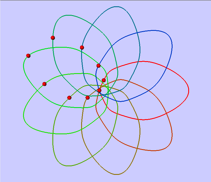
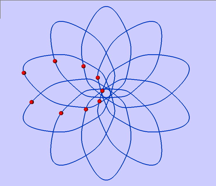
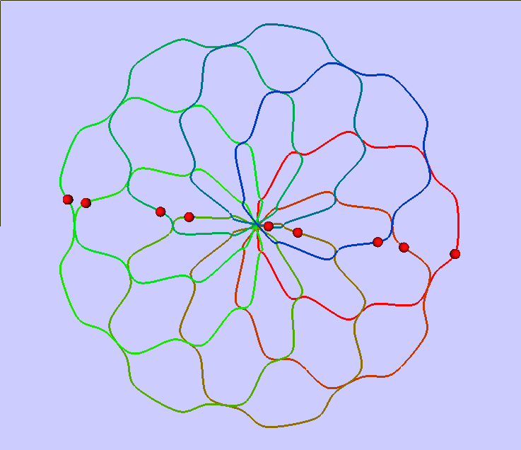
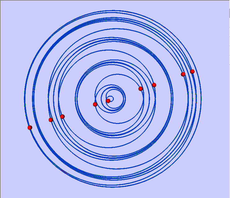
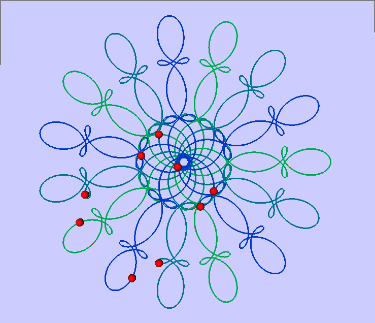
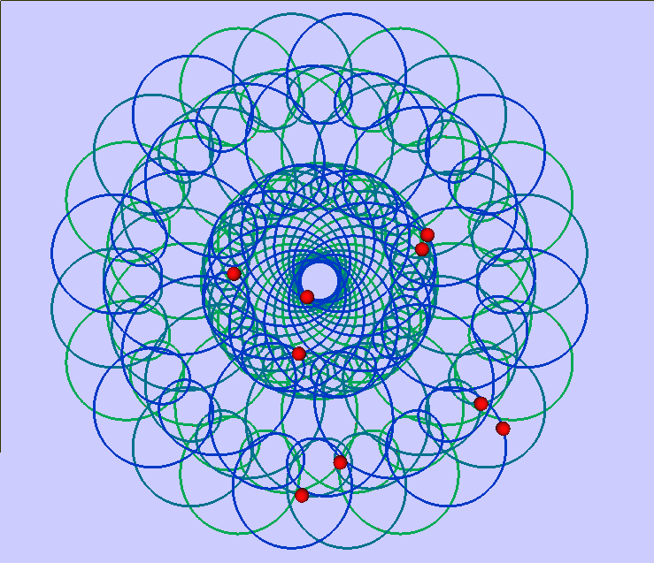
Figure 1: All solutions in this figure are for $n=9$ and, to numerical accuracy, linearly stable. Data are given in Table 1. Top-Left: A periodic solution in the rotating frame, of resonance 1:10. Top-Right: The corresponding periodic solution in the non-rotating frame, where it is a choreography. Center-Left: A periodic solution in the rotating frame, of resonance 23:1. Center-Right: The corresponding choreography. Bottom-Left: A partial choreography in the non-rotating frame, of resonance 2:5. Bottom-Right: A partial choreography in the non-rotating frame of resonance 5:8.

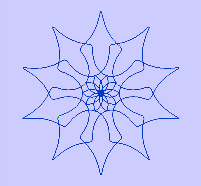
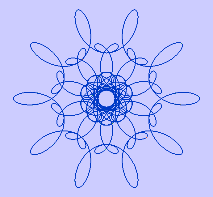
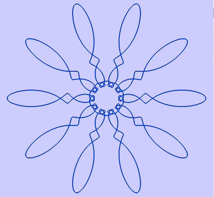
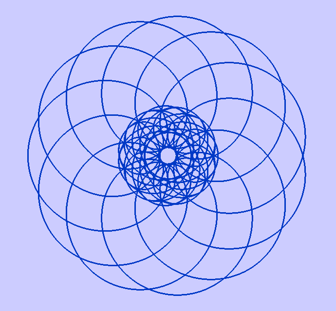
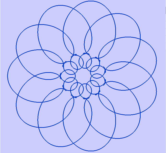
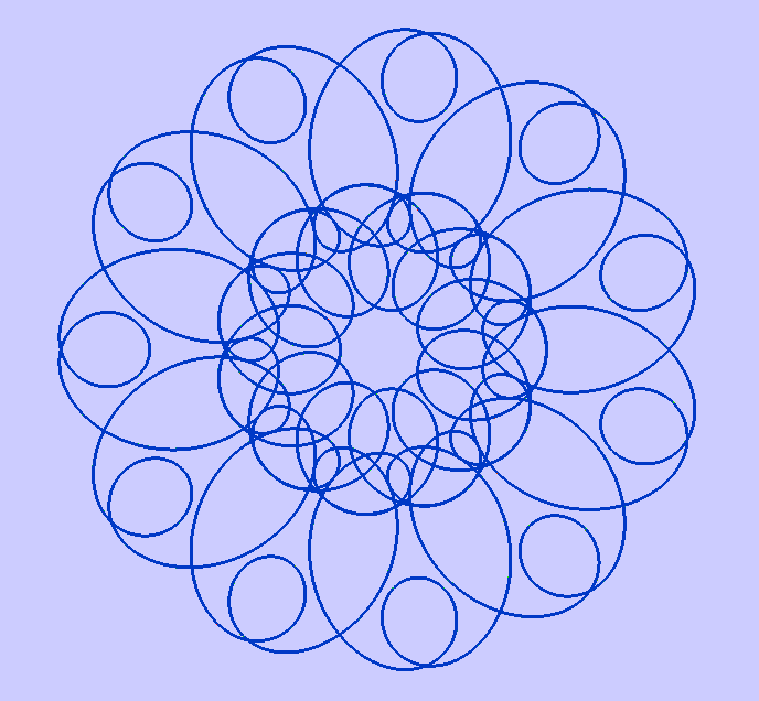
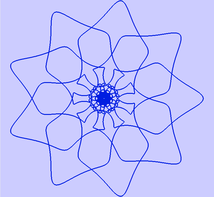
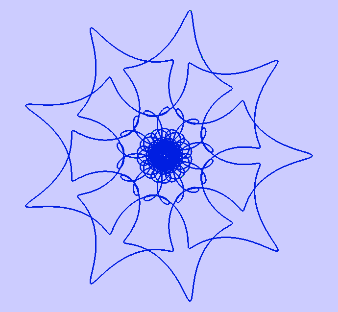
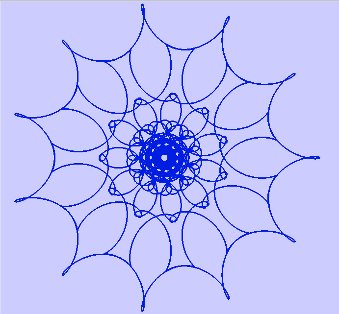
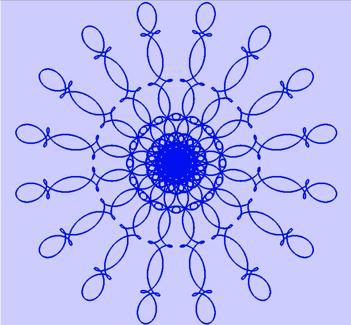
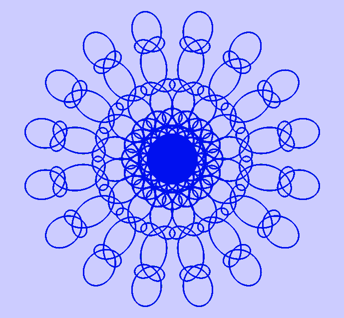
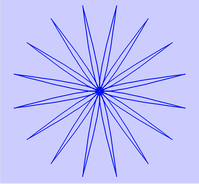
Figure 2: The choreographies in the first two rows are for $n=9$, the choreographies in the third row are for $n=17$, and the choreographies in the last row are for $n=31$. All but two choreographies in this Figure are stable. The two unstable choreographies are on the right in rows 1 and 2.

Figure	Row-	Orbit-	$n$	$T/T_{0}$	a	$T$	$T_{0}$	$x_{n}(0)$	S/U
	Col.	Label
	1-1	1	9	1:10	0.651774	14.5773	145.773	-0.04	S
	1-2	2	9	1:10	0.651774	14.5773	145.773	-0.04	S
1	2-1	3	9	23:1	0.657102	4000.00	173.913	0.005	S
	2-2	4	9	23:1	0.657102	4000.00	173.913	0.005	S
	3-1	5	9	2:5	0.520316	12.7459	31.8649	-0.04	S
	3-2	6	9	5:8	0.396319	12.6334	20.2134	-0.04	S
	1-1	7	9	1:10	0.647930	13.0635	130.635	-0.04	S
	1-2	8	9	1:10	0.646671	12.6423	126.353	-0.04	S
	1-3	9	9	1:10	0.627791	8.51610	85.1505	-0.04	U
	2-1	10	9	2:11	0.510285	5.50498	30.2774	-0.04	S
	2-2	11	9	2:11	0.531986	6.17839	33.9811	-0.04	S
2	2-3	12	9	2:11	0.565906	7.73660	42.5513	-0.04	U
	3-1	13	17	-8:9	0.576588	28.2933	-31.8299	0.005	S
	3-2	14	17	-8:9	0.578005	28.0608	-31.5684	0.005	S
	3-3	15	17	-6:11	0.505528	28.4406	-52.1411	0.005	S
	4-1	16	31	-15:16	0.421561	43.0673	-45.9385	0.0001	S
	4-2	17	31	-15:16	0.421549	43.0706	-45.9420	0.0001	S
	4-3	18	31	-15:16	0.420348	43.3913	-46.2840	0.0001	S

Table 1: Data for the orbits in Figures 1 and 2. Here $n$ is the number of sites, $a$ the amplitude parameter, $T$ the period of the orbit, $T_{0}$ the period of the rotating frame, $x_{n}(0)$ the $x$-component of the $n$th site at time zero, ”S” stands for ”Stable or almost stable”, and ”U” stands for ”Unstable”.

References

- [1] A. V. Borisov, I. S. Mamaev, A. A. Kilin. Absolute and relative choreographies in the problem of point vortices moving on a plane. Regular & Chaotic Dynamics 9, 101-111 (2004).
- [2] T. Bartsch, Q. Dai, B. Gebhard. Periodic solutions of N-vortex type Hamiltonian systems near the domain boundary. arXiv preprint arXiv:1610.04182, 2016 - arxiv.org
- [3] T. Bartsch, Q. Dai. Periodic solutions of the N-vortex Hamiltonian system in planar domains. Journal of Differential Equations 260, 2275-2295 (2016).
- [4] V. Barutello, and S. Terracini. Action minimizing orbits in the n-body problem with simple choreography constraint. Nonlinearity 17, 2015-2039 (2004).
- [5] R. Calleja, E. Doedel, C. García-Azpeitia. Symmetries and choreographies in families bifurcating from the polygonal relative equilibrium of the n-body problem. Preprint submitted (arXiv:1702.03990).
- [6] A. Chenciner and J. Fejoz. Unchained polygons and the -body problem. Regul. Chaotic Dyn. 14 (1), 64-115 (2009).
- [7] A. Chenciner, J. Gerver, R. Montgomery, and C. Simó. Simple Choreographic Motions of N bodies. A preliminary study, in Geometry, Mechanics, and Dynamics, 60th birthday of J.E. Marsden. P. Newton, P. Holmes, A. Weinstein, ed., Springer-Verlag, 2002.
- [8] A. Chenciner and R. Montgomery. A remarkable periodic solution of the three-body problem in the case of equal masses. Ann. of Math. 152(2), 881-901 (2000).
- [9] E. Doedel, E. Freire, J. Galán, F. Muñoz-Almaraz, and A. Vanderbauwhede. Continuation of periodic orbits in conservative and Hamiltonian systems. Phys. D 181, 1-38 (2003).
- [10] D. Ferrario and S. Terracini. On the existence of collisionless equivariant minimizers for the classical -body problem. Invent. Math. 155(2), 305-362 (2004).
- [11] C. García-Azpeitia, J. Ize. Bifurcation of periodic solutions from a ring configuration in the vortex and filament problems. J. Differential Equations 252 (2012) 5662-5678.
- [12] C. García-Azpeitia. Global bifurcation of traveling waves in discrete nonlinear Schrödinger equations. Journal of Difference Equations and Applications (2016). (doi:10.1080/10236198.2016.1210133)
- [13] C. García-Azpeitia and J. Ize. Bifurcation of periodic solutions from a ring configuration of discrete nonlinear oscillators. DCDS-S 6 (2013), 975-983.
- [14] C. García-Azpeitia and J. Ize. Global bifurcation of planar and spatial periodic solutions from the polygonal relative equilibria for the -body problem. J. Differential Equations 254, 2033-2075 (2013).
- [15] T. Kapela and C. Simó. Computer assisted proofs for nonsymmetric planar choreographies and for stability of the Eight. Nonlinearity 20, 1241-1255 (2007).
- [16] P. Kevrekidis. The discrete nonlinear Schrödinger equation. Mathematical Analysis, Numerical Computations and Physical Perspectives, Springer, 2009.
- [17] F. Lederer, G. I. Stegeman, D. N. Christodoulides, G. Assanto, M. Segev, Y. Silberberg. Discrete solitons in optics. Physics Reports 463, 1–126 (2008).
- [18] F. Le Clerc and L. Collot , M. Gross. Numerical heterodyne holography with two-dimensional photodetector arrays. Optics Letters 25, 716-718 (2000).
- [19] R. MacKay and S. Aubry. Proof of existence of breathers for time-reversible or hamiltonian networks of weakly coupled oscillators. Nonlinearity 7 (1994), 1623-1643.
- [20] C. Moore. Braids in Classical Gravity. Physical Review Letters 70, 3675-3679 (1993).
- [21] P. Panayotaros and D. Pelinovsky. Periodic oscillations of discrete NLS solitons in the presence of diffraction management. Nonlinearity 21 (2008), 1265-1279.
- [22] C. Pando and E. Doedel. Bifurcation structures and dominant models near relative equilibria in the one-dimensional discrete nonlinear Schrödinger equation. Physica D. 238 (2009), 687-698.
- [23] D. Pelinovsky and V. Rothos. Bifurcations of travelling wave solutions in the discrete NLS equations. Physica D. 202 (2005), 16-36.
- [24] C. Simó. New Families of Solutions in N-Body Problems. European Congress of Mathematics 101-115. Springer Nature, 2001.
- [25] C. O. Weiss, R. Vilaseca, N. B. Abraham, R. Corbalán, E. Roldán, G. J. de Valcárcel, J. Pujol, U. Hübner, D. Y. Tang. Models, predictions, and experimental measurements of far-infrared NH3-laser dynamics and comparisons with the Lorenz-Haken model. Applied Physics B 61, 223–242 (1995).