A Gaussian process framework for overlap and causal effect estimation with high-dimensional covariates

Abstract

A powerful tool for the analysis of nonrandomized observational studies has been the potential outcomes model. Utilization of this framework allows analysts to estimate average treatment effects. This article considers the situation in which high-dimensional covariates are present and revisits the standard assumptions made in causal inference. We show that by employing a flexible Gaussian process framework, the assumption of strict overlap leads to very restrictive assumptions about the distribution of covariates, results for which can be characterized using classical results from Gaussian random measures as well as reproducing kernel Hilbert space theory. In addition, we propose a strategy for data-adaptive causal effect estimation that does not rely on the strict overlap assumption. These findings reveal the stringency that accompanies the use of the treatment positivity assumption in high-dimensional settings.

Keywords: Average causal effect; Covariate balance; Functional data; Machine learning; Positivity.

1 Introduction

The availability of high-dimensional covariates in administrative databases and electronic health records has led to increasing scientific focus on attempting to evaluate and develop methods for causal inference with these data structures. There has been a concomitant focus in the statistics and econometrics literature towards the use of machine learning-based methods for performing causal inference with high-dimensional data (e.g., van der Laan and Gruber (2010); Van der Laan and Rose (2011); Athey and Imbens (2016), Athey et al. (2018), Chernozhukov et al. (2018)).

In light of this work, it is worth revisiting the standard assumptions necessary for performing causal inference in the potential outcomes framework of Rubin (1974) and Holland (1986). A key assumption that is needed for proper definition of a causal estimand is the unconfoundedness assumption, which states that the treatment is independent of the potential outcomes conditional on confounders. Part of the interest in observational studies with high-dimensional covariates is the belief that sufficiently rich sets of covariates will render the unconfoundedness assumption more plausible.

Another assumption, which is the focus of the current paper, is the treatment positivity assumption, which states that the probability of treatment given covariates is strictly between zero and one for values of the covariate vectors. This is related to the notion of covariate/confounder overlap between the treatment groups. This is taken virtually as a given in most causal analyses, but the emergence of clinical decision support systems, deterministic treatment rules and high-dimensional covariates raises the possibility of this assumption being violated. A simple example of such a violation occurring is a situation in which treatment assignment is made deterministically in a medical setting based on the patient presenting with certain risk factors and comorbidities. In such a case, the treatment positivity assumption would be violated. More generally, Robins and Ritov (1997) have shown that for estimators of the average causal effect to potentially be semiparametrically efficient, the treatment positivity assumption has to be strengthened to the propensity score being uniformly bounded away from zero and one.

Methods for performing causal inference with violations of treatment positivity have been limited in the literature. Crump et al. (2009) characterized its effects in a setting with limited numbers of covariates and developed a simple rule to exclude subjects based on the propensity score. The remaining subjects would be those for whom there is sufficient covariate overlap by which one could make valid causal inference. Traskin and Small (2011) use classification and regression trees (CART) to model group labels derived from the Crump et al. (2009) definition of a study population with sufficient overlap to identify factors by which one can define a study population for which one can make causal inferences about. A recent proposal from Ghosh (2018) suggests defining study populations based on the margin from machine learning algorithms. Another practical approach is to delete observations with extreme propensities close to zero or one, which is known as propensity score trimming. Note that these approaches all estimate a causal parameter that is effectively data-dependent; see Ghosh (2018) for further discussion.

In recent work, D’Amour et al. (2017) studied the notion of strict overlap in the high-dimensional case and described a concept termed strict covariate overlap. This represents one way of extending the treatment positivity assumption into the high-dimensional setting. For this situation, they showed that their covariate overlap assumption implied a bound on the discrepancy between the joint distributions of confounders among the treatment and control groups. The assumption thus places an immediate bound on the difference in joint distributions between treatment and control population. In order to avoid such a restrictive assumption, D’Amour et al. (2017) suggested that one could make sparsity assumptions of several types. First, one could assume sparsity at the level of the propensity score. Second, one could assume the existence of a latent variable that renders treatment independent of the potential outcomes, much as in the standard unconfoundedness assumption. Finally, one could assume the existence of a low-dimensional subspace such that confounders are independent of the potential outcomes conditional on subspace.

Central to the notion of strict overlap is that of bounded likelihood ratio, results for which have been developed by Rukhin (1993, 1997) and exploited by D’Amour et al. (2017). In the current paper, we study the overlap phenomenon using Gaussian processes, which is related to but different from what was done in D’Amour et al. (2017). In particular, we will use the theory of random probability measures, and in particular, random Gaussian measures (Neveu, 1968, Jansson, 1997) to characterize implications of overlap. The line of research we use enjoys a long history in statistical theory, dating back to the results on random measures based on Wiener processes developed by Cameron and Martin (1944, 1945). We show that by assuming a Gaussian process framework, the bounded likelihood ratio result presented in D’Amour et al. (2017) leads to an asymptotic implication of overlap that can be characterized by equivalence and orthogonality of Gaussian measures. These results have been applied to a variety of problems in statistics, including spatial statistics (Stein (2012)) and more recently, classification with functional data (Delaigle and Hall (2012), Berrendero et al. (2018)). The applications of these results to the causal inference setting are new.

Next, we show that for a specific Gaussian process model, a phase transition phenomenon exists with respect to the overlap assumption that can be characterized in terms of the component eigenvalues and eigenfunctions. This will entail the use of and summarizing results from Delaigle and Hall (2012) and Berrendero et al. (2018). The practical implication of these results are manifold:

1. For causal inference with high-dimensional covariates, the Gaussian process framework reveals that assuming treatment positivity is equivalent to assuming equivalence of the probability laws of the confounders given treatment groups;

2. If equivalence does not hold, then one has that the probability laws of the confounders given treatment groups are orthogonal measures, which represents a complete violation of overlap;

3. We show how one can develop a causal effect estimation strategy that is less reliant on the covariate overlap assumption. It extends the work of Ghosh (2018) for estimating data-adaptive causal estimands based on the margin.

The structure of this paper is as follows. In Section 2, we review the potential outcomes model, previous work on covariate overlap as well as provide a review on Gaussian processes. The latter will prove useful in the framework that we describe in Section 3. In Section 4, some practical implications for causal modelling approaches are provided, along with an extension of the strategy from Ghosh (2018) to incorporate covariance structures. Some discussion concludes the paper in the last section.

2 Background

2.1 Preliminaries and Causal inference assumptions

In this paper, we will employ the potential outcomes framework of Rubin (1974), Holland (1986), which has been widely used in causal modelling. Throughout, we denote the set $\{1,\dots,n\}$ by $[n]$. We start by assuming an underlying probability space $\left(\Omega,\Sigma,\mathbb{P}\right)$, and random variables $Z:\left(\Omega,\Sigma,\mathbb{P}\right)\rightarrow\left(\mathcal{Z},\Sigma_{\mathcal{Z}}\right)$, $Y:\left(\Omega,\Sigma,\mathbb{P}\right)\rightarrow\left(\mathcal{Y},\Sigma_{\mathcal{Y}}\right)$, and $T:\left(\Omega,\Sigma,\mathbb{P}\right)\rightarrow\left(\mathbb{B},\Sigma_{\mathbb{B}}\right)$, where $\mathbb{B}:=\{0,1\}$, and $\mathcal{Z}$, $\mathcal{Y}$ are the confounder and response spaces, respectively. The derived distribution of $Z$ is defined as $P_{\mathbf{Z}}:=\mathbb{P}\circ Z^{-1}$. We define $P_{\mathbf{Y}}$ and $P_{\mathbf{T}}$ analogously. $Y$ denotes the response of interest and ${Z}$ is a $p$-dimensional vector of confounders. $T$ is a binary indicator of treatment exposure, where $T=1$ if treated and $T=0$ if control. We denote their joint distribution by $P$, and assume the observed data, represented as $\{(Y_{i},{Z}_{i},T_{i})\}_{i\in[n]}$, is drawn from $P$. Note that, in this section, we will assume the confounders are simply a finite-dimensional vector.

Let $\{Y_{i}(0),Y_{i}(1)\}$ be the potential outcomes for subject $i$, $i\in[n]$, where $Y_{i}(0)$ refers to the potential outcome under control and $Y_{i}(1)$ to that under treatment. We further assume our observation $Y_{i}$ has the form $Y_{i}:=Y_{i}(T_{i})=Y_{i}(1)T_{i}+Y_{i}(0)(1-T_{i})$, which is commonly referred to as the consistency assumption in the causal inference literature.

In an observational study, the vector of covariates ${Z}$ could be related to both the outcome and the treatment assignment. Since both $T$ and the potential outcomes {Y(0),Y(1)} are affected by ${Z}$, $T\perp\{Y(0),Y(1)\}$ will not hold. To enable causal inference in this scenario, we make the following further assumptions.

1. Strongly Ignorable Treatment Assumption (SITA): $\{Y(1),Y(0)\}$ is independent of $T$ given ${Z}$.

2. Stable Unit Treatment Value Assumption (SUTVA): The potential outcomes for subject $i$ is statistically independent of the potential outcomes for all subjects $j\neq i$, for $i,j\in[n]$.

3. Treatment Positivity Assumption (TP): $P_{\mathbf{T}|\mathbf{Z}}(T=1|{Z})>0$ for all values of ${Z}$.

Taking these assumptions in order, SITA means that by conditioning on $Z$, the observed outcomes can be treated as if they come from a randomized complete block design. Rosenbaum and Rubin (1983) show that if SITA holds, then the treatment is independent of the potential outcomes given the propensity score, defined as

$$e(Z):=P_{\mathbf{T}|\mathbf{Z}}(T=1|{Z}).$$

Robins and Ritov (1997) uses the terminology ‘no unmeasured confounders’ in lieu of SITA. The TP assumption was described in the Introduction and will be considered further in the next section.

In passing, we mention that the typical parameter of focus in causal analyses is the average causal effect (ACE), defined as

$$ACE:=E(Y(1)-Y(0)),$$ (1)

where the expectation is taken with respect to the joint distribution of $Y_{i}(0)$ and $Y_{i}(1)$. The use of propensity score modelling (Rosenbaum and Rubin, 1983) in conjunction with outcome regression modelling leads to a variety of approaches to average causal effect modelling, a comprehensive overview on the topic being Imbens and Rubin (2015).

2.2 Review of previous work regarding treatment positivity and covariate overlap

We focus on the treatment positivity assumption and describe previous work in this area. Crump et al. (2009) noted the possibility that treatment positivity could be violated and instead defined a subpopulation causal effect using the propensity score. Let $\mathbf{I}(C)$ denote the indicator function for the event $C$. Define the region ${\cal A}:=\{{Z}:c\leq e({Z})\leq 1-c\}$ for some $c>0$. Note we suppress the explicit dependence of ${\cal A}$ on $c$. Crump et al. (2009) define the subpopulation average causal effect as

$${ACE_{\cal A}}:=\frac{\sum_{i=1}^{n}\mathbf{I}(\{e({Z}_{i})\in{\cal A}\})\left(Y_{i}(1)-Y_{i}(0)\right)}{\sum_{i=1}^{n}\mathbf{I}(\{e({Z}_{i})\in{\cal A}\})}.$$

Note the dependence of ${ACE_{\cal A}}$ on the region of the propensity scores that is in ${\cal A}$. In practice, ${\cal A}$ must be estimated from the data, and this is done by estimating the propensity score to obtain $\hat{e}(Z_{i})$, $i=1,\ldots,n$. By plugging in $\hat{e}(Z_{i})$ instead of $e(Z_{i})$ in the definitions of $\mathcal{A}$ and $ACE_{\mathcal{A}}$, we obtain $\widehat{\cal A}$ and $\widehat{ACE}_{{\cal A}}$, respectively. We finally employ $\widehat{ACE}_{\widehat{\cal A}}$ as our final estimator. Based on the variability of the estimated subpopulation average causal effect, Crump et al. (2009) proposed an optimization criterion for determining an optimal cutoff value in the definition of ${\cal A}$ and demonstrated under some mild assumptions that an optimal $c^{*}$ exists. The optimal value depends only on the marginal distribution of the propensity scores.

Traskin and Small (2011) developed a meta-approach for characterizing treatment positivity using classification and regression trees (Breiman et al., 1984). In general, a tree classifier works as follows: beginning with a training data set $\{({Z}_{i},T_{i})\}_{i\in[n]}$, drawn from the joint distribution of $Z$ and $T$, a tree classifier repeatedly splits nodes based on one of the covariates in ${Z}$, until it stops splitting by some stopping criteria (for example, the terminal node only contains training data from one class). Each terminal node is then assigned a class label by the majority of subjects that falls in that terminal node. Once a testing data point with a covariate vector ${Z}$ is introduced, the data point is run from the top of the tree until it reaches one of the terminal nodes. The prediction then will be made by the class label of that terminal node. Compared to parametric algorithms, tree-based algorithms have several advantages. There is no need to assume any parametric model for a tree; the algorithm for its constructions only requires a criterion for splitting a node and a criterion for when to stop splitting (Breiman et al., 1984). Traskin and Small (2011) propose a modelling approach in which one develops a class label for subject $i$ depending on whether or not $\hat{e}(Z_{i})\in\widehat{\cal A}$, $i\in[n]$. Define $Y^{*}_{i}:=\mathbf{I}(\hat{e}(Z_{i})\in\widehat{\cal A})$, $i\in[n]$. Traskin and Small (2011) then propose fitting a tree model for $Y^{*}_{i}$ on $Z_{i}$ to determine the covariates that explain being in the overlap set of Crump et al. (2009). We term this a ‘meta-approach’ because the modeling is being based on a response variable that is derived using the estimated propensity score.

On the theoretical front, Khan and Tamer (2010) demonstrated that if the TP assumption is violated, then irregularities regarding identification and inference about causal effects can occur. This has echoes in the work of Robins and Ritov (1997), who show that to have regular semiparametric estimators for average causal effects in the high-dimensional case, the model classes for the propensity score and outcome models have to be well-behaved. Thus, violations in standard overlap assumptions lead to irregularities in estimation and inference. This was noted in Luo et al. (2017), who found that by assuming a weaker covariate overlap assumption, one could derive an estimator that exhibited super-efficiency (i.e, having an information bound that is smaller than the classical semiparametric information bound for regular estimators). This phenomenon also occurs in the collaborative targeted maximum likelihood estimator of van der Laan and Gruber (2010). The problem with superefficient estimators, as noted by D’Amour et al. (2017), is that for model directions where the relaxed assumptions do not hold, the estimators can have unbounded loss functions.

D’Amour et al. (2017) consider the problem of covariate overlap in one high-dimensional setting. Define the conditional probabilities $P_{\ell}(Z):=P_{\mathbf{Z}|\mathbf{T}}(Z|T=\ell)$, $\ell\in\mathbb{B}$, and denote their Radon-Nikodym derivatives with respect to $P_{\mathbf{Z}}$ as $f_{\ell}:=dP_{\ell}/dP_{\mathbf{Z}}$. Let $\alpha=P_{\mathbf{T}}(T=1)$ and note $P_{\mathbf{Z}}=\alpha P_{1}+(1-\alpha)P_{0}$. They note that the strict overlap assumption:

$$\eta\leq e(Z)\leq 1-\eta\ \ \ \ \ \text{almost everywhere }P_{\mathbf{Z}}$$ (2)

for some $\eta\in(0,0.5)$, is equivalent to the following bounded likelihood ratio assumption: for $P_{\mathbf{Z}}$-almost all $z\in\mathcal{Z}$:

$$\frac{\eta}{1-\eta}\leq\frac{\alpha}{1-\alpha}LR(z)\leq\frac{1-\eta}{\eta}$$ (3)

where $LR(z):=f_{1}(z)/f_{0}(z)$ is the likelihood ratio of the treatment to the control populations. For the sake of completeness, we provide a straightforward proof in the appendix, since none was given in the original paper. We note assumption (3) is a bounded likelihood ratio assumption. This allows D’Amour et al. (2017) to exploit results from information theory (Rukhin, 1993, 1997) to show that (3) imposes limits on the rate of growth of discriminatory information between the joint distributions of confounders in the treatment and control populations. Interestingly, these bounds are independent of $p$, the number of confounders. From an intuitive point of view, this makes sense, for when the number of covariates increase, one would expect that the probability of random classifiers to perfectly separate the data between the treatment and control populations would increase. This proves problematic for the causal inference problem, as it leads to a violation of the TP assumption.

2.3 Review of Gaussian Processes

We now consider the case where $Z$ is a Gaussian process instead of a finite-dimensional Gaussian variable. $Y$ and $T$ remain as in the previous section but now $Z:\left(\Omega,\Sigma,\mathbb{P}\right)\rightarrow\left(\mathcal{Z}(\mathcal{T}),\Sigma_{\mathcal{Z}}\right)$ where $\mathcal{Z}(\mathcal{T})$ is a suitable function space on $\mathcal{T}$. To simplify things we can assume these functions are real-valued. It will be more useful to understand $Z$ in the following way: write $Z(\omega,\cdot)$ for the elements of $\mathcal{Z}(\mathcal{T})$, and define the maps $\pi_{t}(Z):=Z(\cdot,t)\,\,\,\forall t\in\mathcal{T}$. Then, $Z_{t}:=\pi_{t}\circ Z$ are functions from $\Omega$ to $\mathbb{R}$. Indeed, each of these functions is a random variable if and only if $Z$ is also a random variable. Indeed $Z$ is fully determined by $\{Z_{t}\}_{t\in\mathcal{T}}$ and, furthermore, its distribution is fully determined by the finite dimensional joint distributions $\{Z_{t_{i}}\}_{i\in n}$ for all collections $\{t_{i}\}_{i\in n}$ and all $n$. When such distributions are all Gaussian, $Z$ is a Gaussian process. If $Z_{t}$ is square-integrable for all $t\in\mathcal{T}$, we call $Z$ a second-order process, throughout the paper we assume $Z$ is second-order. Comprehensive reviews of Gaussian processes can be found in Neveu (1968) and Jansson (1997).

2.3.1 Associated Hilbert space

For simplicity, we assume here that $E(Z_{t})=0$ for all $t\in\mathcal{T}$, although this assumption will be relaxed later in the paper. Gaussian Processes can be characterized by their covariance function, given by

$$k(s,t)=\text{Cov}\{Z_{s},Z_{t}\},\ \ \ \ (s,t)\in{\cal T}\times{\cal T}.$$

For a second-order Gaussian Process, the covariance function $k$ will be a symmetric and positive definite function on ${\cal T}\times{\cal T}$. Well known results from functional analysis ensure each function $k$ of such type is in one-to-one correspondence to a Hilbert space $\mathcal{H}_{k}$ with the following reproducing property:

$$\langle\,f,k(\cdot,t)\,\rangle_{\mathcal{H}_{k}}=f(t),\,\,\,\forall f\in\mathcal{H}_{t}.$$

In lieu of the reproducing property, We call $\mathcal{H}_{k}$ the reproducing kernel Hilbert space (RKHS) of $k$, and $k$ the reproducing kernel of $\mathcal{H}_{k}$. For details see Berlinet and Thomas-Agnan (2011), Aronszajn (1950)

2.3.2 Equivalence of distributions

Definition. Two measures $\mu_{0}$ and $\mu_{1}$ defined on a probability space $(X,\mathcal{X})$ are said to be mutually singular (or orthogonal), denoted by $\mu_{0}\perp\mu_{1}$, if there exists a set $A\in{\cal X}$ such that $\mu_{0}(A)=0$ and $\mu_{1}(X\backslash A)=0$. $\mu_{0}$ and $\mu_{1}$ are said to be mutually equivalent (or equivalent), denoted by $\mu_{0}\sim\mu_{1}$, if for all $A\in{\cal X}$, $\mu_{0}(A)=0\Leftrightarrow\mu_{1}(A)=0$.

It is well-known from probability theory that two Gaussian measures defined on the same measure space will either be orthogonal or equivalent (Hajek, 1958, Feldman, 1958). Assume $\mu$ to be a measure that dominates both $\mu_{0}$ and $\mu_{1}$ (e.g., $\mu=\mu_{0}+\mu_{1}$). Define $d\mu_{0}/d\mu$ and $d\mu_{1}/d\mu$ to be the Radon-Nikodym derivatives associated with $\mu_{0}$ and $\mu_{1}$, respectively. Furthermore, define

$$B:=\int\sqrt{\frac{d\mu_{1}}{d\mu}\frac{d\mu_{0}}{d\mu}}d\mu$$

and

$$J:=\int\left(\frac{d\mu_{0}}{d\mu}-\frac{d\mu_{1}}{d\mu}\right)\log\left(\frac{d\mu_{0}/d\mu}{d\mu_{1}/d\mu}\right)d\mu.$$

Note that $B$ is the Bhattacharya coefficient between two probability measures and $J$ is the relative entropy. Several authors have developed characterization results for orthogonality and equivalence of Gaussian measures in terms of $B$ and $J$ (Hajek, 1958, Rao and Varadarajan, 1963, Shepp, 1966) We summarize them here using Theorem 1 from Shepp (1966).

Theorem 1 (Theorem 1 of Shepp (1966))

(a). $\mu_{0}\perp\mu_{1}$ if and only if $B=0$ or $J=\infty$.

(b). $\mu_{0}\sim\mu_{1}$ if and only if $B>0$ or $J<\infty$.

If $\{\mu_{0}^{(n)}\}$ and $\{\mu_{1}^{(n)}\}$ are sequences of Gaussian measures with corresponding Bhattacharya and relative entropy sequences $\{{B}_{n}\}$ and $\{J_{n}\}$ converging to $B$ and $J$, then Theorem 1 suggests there are two asymptotic scenarios for Gaussian measures as $n$ approaches infinity. They are either asymptotically orthogonal (part (a)) or equivalent (part (b)).

While the Gaussian process assumption may seem restrictive at first glance, we note that they in fact represent a very flexible class of probability models to fit to data. They have been widely used in Haran (2011) for spatial statistics, Kennedy and O’Hagan (2001) for designs of computer experiments and by Williams and Rasmussen (2006) for machine learning.

3 Proposed framework

3.1 Overlap assumptions and Gaussian Processes

As before, we represent the random measures for $Z|T=1$ and $Z|T=0$ by $P_{1}$ and $P_{0}$, respectively. We now reconsider the assumptions of causal inference for $Z$ a Gaussian process. The functional version of unconfoundedness can be given by

$$T\perp\{Y(1),Y(0)\}|{\cal F}_{\mathcal{Z}},$$

where ${\cal F}_{\mathcal{Z}}:=\sigma(Z_{t}:t\in\mathcal{T})$ denotes the smallest $\sigma-$algebra for which every $Z_{t}$ is measurable.

The assumption of SUTVA remains the same as described in §2. Finally, the treatment positivity assumption can be written as

$$0<P(T=1|Z)<1\text{ almost everywhere}\ \ P_{\mathbf{Z}}.$$

Analogously to (3) we define strict functional overlap to be

$$\frac{\eta}{1-\eta}<\frac{\alpha}{1-\alpha}\frac{dP_{1}/dP(z)}{dP_{0}/dP(z)}<\frac{1-\eta}{\eta},$$ (4)

for almost-all $z\in\mathcal{Z(\mathcal{T})}$ and for $\eta\in(0,.5)$. This is identical to the bounded likelihood ratio assumption of D’Amour et al. (2017).

Define $\{P^{(n)}_{0}\}$ and $\{P^{(n)}_{1}\}$ to be the restrictions of $P_{0}$ and $P_{1}$, respectively, to the smallest $\sigma-$algebra for which $\{Z_{1},\ldots,Z_{n}\}$ is measurable. Let the means be denoted as $\{m^{(n)}_{0}\}$ and $\{m^{(n)}_{1}\}$. We have the following result:

Theorem 2

Assumption (4) implies that $P_{0}\sim P_{1}$.

Proof: Using integration, one can show that

$$B(P^{(n)}_{0},P^{(n)}_{1})=\frac{1}{4}L_{n}+\frac{1}{8}D^{2}_{n},$$

where

$$L_{n}=2\log|\Lambda_{n}|-\log|\Lambda_{0n}|-\log|\Lambda_{1n}|,$$

with $\Lambda_{jn}$ denoting the covariance operator in $n-$dimensional space for group $j$ $(j=0,1)$ and $\Lambda_{n}=(\Lambda_{0n}+\Lambda_{1n})/2$. The term $D^{2}_{n}:=\left(m_{1}^{(n)}-m_{0}^{(n)}\right)^{\prime}\Lambda^{-1}_{n}\left(m_{1}^{(n)}-m_{0}^{(n)}\right)$ represents the Mahalanobis distance in $n-$dimensional space. By Theorem 3.2 of Rao and Varadarajan (1963), we have that

$$B(P_{0},P_{1}) = \lim_{n\rightarrow\infty}B(P^{(n)}_{0},P^{(n)}_{1})$$

$$= \lim_{n\rightarrow\infty}\frac{1}{4}L_{n}+\frac{1}{8}D^{2}_{n}.$$

As noted in Rao and Varadarajan (1963), $L_{n}/4$ represents the Hellinger distance between two zero-mean multivariate normal distributions, one with covariance $\Lambda_{0n}$, the other with covariance $\Lambda_{1n}$. Similarly, $D^{2}_{n}/8$ is the Hellinger distance between two $n-dimensional$ multivariate normal distributions with means $m_{0}^{(n)}$ and $m_{1}^{(n)}$ and common covariance $\Lambda_{n}$. Now, note that $L_{n}$ and $D_{n}$ are both greater than equal to zero for all $n$ and are increasing with $n$ The assumption (4), which is a bounded likelihood ratio assumption implies that $L_{n}$ and $D^{2}_{n}$ are uniformly bounded away from zero and infinity for all $n$. Thus, their limits will also be greater than zero so that $B(P_{0},P_{1})>0$. We can thus use Theorem 1(b) to conclude equivalence. This concludes the proof of Theorem 2. $\blacksquare$

3.2 Reinterpretation using RKHS theory and phase transition

We showed in §2.2. how a Gaussian stochastic process can be used to define an RKHS. In this section, we will assume that $P_{0}$ and $P_{1}$ represent the probability laws of Gaussian processes with mean functions $m_{0}$ and $m_{1}$, respectively, and shared covariance function $k$. We further assume $m_{0}=0$ and $m_{1}$, and $k$ are continuous in their respective domains. If $\mathcal{T}$ is compact, then $k$ is a Mercer kernel and it admits an expansion of the form

$$k(s,t)=\sum_{j=1}^{\infty}c_{j}\psi_{j}(s)\psi_{j}(t),$$ (5)

where for $j=1,2,\ldots$, $\{c_{j}\}$ and $\{\psi_{j}\}$ denote the eigenvalues and eigenfunctions of the integral operator associated to $k$. For details on such operators, refer to Steinwart et al. (2006). Based on the decomposition (5), we can decompose the signal $m_{1}$ as

$$m_{1}(t)=\sum_{j=1}^{\infty}a_{j}\psi_{j}(t).$$

Recently, Delaigle and Hall (2012) and Berrendero et al. (2018) have studied and developed this as a model for classification with functional data. These authors referred to the problem as one of ‘near-perfect’ classification of functional data. Of relevance is a quote by Delaigle and Hall (2012): ‘these (functional classification) problems have unusual, and fascinating properties that set them apart from their finite-dimensional counterparts. In particular, we show that in many quite standard settings, the performance of simple (linear) classifiers constructed from training samples becomes perfect as the sizes of the samples diverge….That property never holds for finite-dimensional data, except in pathological cases.”

Delaigle and Hall (2012) and Berrendero et al. (2018) developed technical characterizations of the ‘near-perfect’ classification phenomenon. In the context of our discussion, the work of Berrendero et al. (2018) is perhaps the most relevant. We have the following theorem.

Theorem 3

(a). If (4) holds, then $\sum_{j=1}^{\infty}c_{j}^{-1}a_{j}^{2}<\infty$.

(b). If $\sum_{j=1}^{\infty}c_{j}^{-1}a_{j}^{2}=\infty$, then (4) cannot hold.

Proof: We first begin with the proof of Theorem 3a. By Theorem 2, if (4) holds, then $P_{1}\sim P_{0}$. By Theorem 5a of Berrendero et al. (2018), this is identical to

$$\sum_{j=1}^{\infty}c_{j}^{-1}a_{j}^{2}<\infty.$$

For the proof of Theorem 3b, by Theorem 4b of Berrendero et al. (2018), $\sum_{j=1}^{\infty}c_{j}^{-1}a_{j}^{2}=\infty$ is identical to $P_{1}\perp P_{0}$. Note that for probability measures $P_{1}\perp P_{0}$ implies $P_{0}$ and $P_{1}$ are not mutually equivalent. Hence, by contraposition of Theorem 2, Assumption (4) cannot hold. $\blacksquare$

Theorem 3 captures a certain type of phase transition in the functional covariate overlap behavior based on the properties of the operator associated to $k$. In particular, the squared eigenvalues of the mean signal divided by the eigenvalues for the kernel operator, characterize strict functional overlap. If strict functional overlap holds, the summation converges (Theorem 3a), while divergence of the series (Theorem 3b) implies strict functional overlap not holding. The results of Theorem 3 are usable in situations where we can derive an explicit Mercer expansion for $k$ in the form of (5). If the $\{\psi_{n}\}$ represent a countably infinite set of orthonormal basis functions, then $\{a_{n}\}\ \ (n\geq 0)$ corresponds to the spectrum of $k$, and if $k$ in (5) is symmetric and positive definite, then $a_{n}\geq 0$ for all $n$. We now give some examples on the application of Theorem 3.

Example. Suppose we set $k$ to be the Gaussian kernel in one dimension:

$$k(x,y)=\exp\{-(x-y)^{2}/2\sigma^{2}\},$$

where $x$ and $y$ are scalars, $\sigma^{2}$ represents a scale parameter. In Steinwart et al. (2006), the authors show how to represent the Gaussian kernel in the form (5), with

$$c_{n}=\sqrt{\frac{2\sigma^{2n}}{n}},\ \ \ \ \psi_{n}(x)=x^{n}\exp(-\sigma^{2}x^{2}).$$

By Theorem 3a, if (4) holds, then

$$\sum_{j=1}^{\infty}c_{j}^{-1}a_{j}^{2}<\infty.$$

In addition, if

$$\sum_{j=1}^{\infty}c_{j}^{-1}a_{j}^{2}=\infty,$$

then (4) cannot hold. Noting that the summation will converge if $c_{j}^{-1}a_{j}^{2}=j^{-(1+\epsilon)}$ for some $\epsilon>0$, some algebra yields that this is equivalent to

$$a_{j}=\sigma^{-j/2}j^{-1/2(1/2+\epsilon)}$$

for $j\geq 0$. Recalling the definition of $a_{j}$, this places an immediate constraint on the mean function $m_{1}(t)$.

4 Practical Implications for Causal inference

While the results presented so far have been of a relatively theoretical nature, one practical implication of the results in Section 3 is that with high-dimensional covariates, there is a strong tension and interplay between (a) maintaining a treatment positivity assumption and (b) having the ability to compute causal effect estimators that are semiparametrically regular in the sense of Robins and Ritov (1997). One common practice for causal effect estimation is the following strategy:

1. Fit a propensity score model for treatment given covariates;

2. Evaluate covariate balance between the treatment groups, taking into account the propensity scores. If balance does not hold, modify step 1.

3. Estimate the causal effect of interest incorporating the propensity score.

If a propensity score model can perfectly predict treatment, then we are in a situation where there the treatment positivity assumption is violated. Thus, for causal modelling to proceed, one would need stronger assumptions to hold. For example, targeted learning approaches also fit a model for the potential outcomes, and if that model is correctly specified, then this would overcome the issue of violation of treatment positivity. More fundamentally, the violations in overlap necessitate the use of data-adaptive causal effect estimation approaches, which we describe in the next section.

4.1 Data-adaptive causal effect estimation

A recent innovation for attempting to relax some of the overlap assumptions is the margin-based approach of Ghosh (2018). The intuitive idea of that work is to first identify the margin and then conditional on the margin, develop causal effect estimation and inference procedures. This is related to, but different from, the finding in D’Amour et al. (2017) that a set of observations where propensity score model misclassifications occur (i.e., the predicted treatment assignment is not concordant with the observed treatment assignment) represent a set of individuals which might be concordant with the treatment positivity assumption.

We consider the binary treatment scenario and recode treatment as $-1$ and $1$ and use support vector machines (SVM; Cristianini et al. (2000)) to fit a propensity score model for treatment. The objective of SVM is to find a hyperplane, in an appropriate high-dimensional space, that maximizes the margin between the populations defined by $T=1$ and $T=-1$. One approach to mapping data into a high-dimensional space is through use of the so-called ‘kernel trick’, which corresponds to using RKHS to define support vector machines. Using a loss function framework, we can characterize the optimization problem as finding to $f$ to minimize

$$\sum_{i=1}^{n}|1-T_{i}f(Z_{i})|_{+}\ \ +\lambda\|f\|^{2}_{K},$$

where $|a|_{+}=\max(a,0)$, $\lambda>0$ denotes a smoothing parameter and $\|f\|_{K}$ denotes the norm of a function $f$ in an RKHS with associated kernel $K$. At a high level, the approach being proposed here amounts to the following:

1. Fit a support vector machine with kernel $K$ to the data $(T_{i},{\bf X}_{i})$, $i=1,\ldots,n$;

2. Determine the observations that are in the margin; denote these as ${\cal M}$;

3. Estimate the causal effect of interest using $(Y_{i},T_{i},{\bf X}_{i})$, $i\in{\cal M}$;

Extending the arguments of Theorem 1 in Ghosh (2018), the margin for nonlinear support vector machines based on a kernel $K$ can be viewed as satisfying a functional version of relaxed covariate overlap. The relaxed covariate overlap notion is detailed more clearly in Ghosh (2018) and as the name suggests, is meant to be a relaxation of the standard covariate overlap assumption in causal inference.

4.2 Numerical example

As an example, we consider the SUPPORT study from Connors et al. (1996), a version of which was previously analyzed in Ghosh et al. (2015). The causal effect of interest is the effect of right heart catherization (RHC) on 30-day survival (dead/alive at 30 days). The dataset contains information on 5735 patients, 2184 of whom received RHC. Note that the covariates are a mixture of continuous as well as discrete variables, so the assumption of a Gaussian process for the data may not be terribly realistic. Determining the robustness of results to this assumption is an important topic for future work.

We employed the implementation of support vector machines as available in the R e1071 package based on the Gaussian kernel:

$$K(x,y)=\exp(-\|x-y\|^{2}/2\sigma^{2}),$$

where $x$ and $y$ are $p-$dimensional vectors, and $\sigma>0$ is a scale parameter. Out of the original 5735 subjects, 3663 are selected to be in the margin, and based on these subjects, the average causal effect is estimated to be 0.049 with an associated standard error of 0.016, which yields a highly significant effect. Thus, the use of RHC is associated with decreased probability of 30-day survival, or conversely, increased risk of death within 30 days. Because of the sensitivity of $K$ to the choice of $\sigma^{2}$, we performed sensitivity analyses in which we varied $\sigma^{2}$ and reran the analysis. In all instances, we found a positive average causal effect. This aligns with the findings in Connors et al. (1996).

We also used the methodology of Traskin and Small (2011) to better understand how the margin population was selected. The plot of the tree is given in Figure 1.

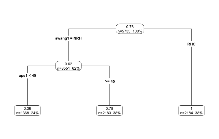
Figure 1: Tree plot from modelling being in the margin as a function of the covariates in the SUPPORT study. The tree was pruned using a cost-complexity parameter of 0.1.

Based on Figure 1, we find that all the subjects treated with right-heart catheterization are included in the margin. In addition, patients with higher APACHE scores, which correlate with higher mortality, are much more likely to be included in the margin.

5 Discussion

In this article, we have studied the covariate overlap assumption using Gaussian processes. The results here complement those in D’Amour et al. (2017). The way in which high-dimensional covariates are considered is different from that paper. There, they consider the situation of $p$, the number of confounders, approaching infinity. By contrast, here, we use a Gaussian random measure to represent a theoretically infinite-dimensional confounder. An implication of the analysis here is that the treatment positivity assumption is not as innocuous as it seems, which is similar to the conclusion reached by D’Amour et al. (2017).

We also point out that virtually all proposals that are available for causal effect estimation assume a covariate overlap assumption or equivalently, the propensity score being bounded away from zero and one uniformly in the confounders. Letting $n$ denote the sample size and $p$ the dimension of the confounders, this could be in a ‘large n, small p’ case (e.g., Chan et al. (2016)) or in a ‘large p, small n’ setup (e.g., Athey et al. (2018)). Our results suggest that for the latter case, the covariate overlap assumption leads to restrictive assumptions on the distributions of confounders between the treatment groups and that any discrepancy vanishes asymptotically. If such an assumption is not plausible, then this effectively renders impossible the possibility of average causal effect estimators achieving $n^{1/2}$ convergence (Robins and Ritov, 1997). In their words, relaxing the assumption of overlap in the high-dimensional case allows for ‘pathological’ distributions to be considered as part of the model class, and these distributions have the possibility of leading to causal effect estimators with irregular behavior (e.g., superefficiency). The estimators in Luo et al. (2017) and van der Laan and Gruber (2010) fall into this class.

This article synthesized several results on Gaussian measures that have been in the literature over the last 70 years. One of the limitations of this article is that the types of covariates that are treated here as being functional are indexed by a one-dimensional set (e.g., time). An example of biomedical data that could be treated as functional in nature are longitudinal data in electronic medical records, but many covariates in practice might not fit this structure. Understanding the robustness of the results presented in this paper to violations of the Gaussian process assumption are beyond the scope of the current manuscript and a topic for future research.

The paper addresses the issue of equivalence versus orthogonality with Gaussian measures for causal inference problems. In practice, it is difficult to verify if the strict overlap criteria in this article actually hold. This suggests that approaches that can accommodate violations should be considered. Petersen et al. (2012) discussed possible violations of the treatment positivity assumption along with potential causes and tools to evaluate their effects in terms of biases of causal effect estimates. Suggestions there include restricting the space of treatments, redefining the causal estimand, and using alternative projection functions. We have proposed redefining the estimand in Section 4.1. Furthering work in these areas will be necessary in order to advance the use of these analytic approaches for causal effect estimation with high-dimensional confounders.

The recent use of deep learning techniques for learning representations in causal inference has also been proposed by Johansson et al. (2016). Extension of the results in Section 3 to the deep learning case would also be of major interest. Dunlop et al. (2018) have studied ‘deep’ Gaussian processes, which consist of a recursive definition for the Gaussian process based on a Markov chain. It would be of interest to extend equivalence results to that setting as well.

Appendix

Proof of Equation (3)

We will prove the right hand side inequality only, as the left hand side inequality is proven analogously. The strict overlap assumption is: $P_{\mathbf{T}|\mathbf{Z}}(T=1|Z)\leq\eta$ almost everywhere $P_{\mathbf{Z}}$. Hence, by Bayes rule:

$$\frac{P_{\mathbf{Z}|\mathbf{T}}(Z|T=1)P_{\mathbf{T}}(T=1)}{P_{\mathbf{Z}}(Z)}\leq\eta,$$

or, using the notation around equation (3):

$$\frac{\alpha P_{1}(Z)}{\alpha P_{1}(Z)+(1-\alpha)P_{0}(Z)}\leq\eta\,\,\, \implies$$

$$\alpha P_{1}(Z)\leq\eta(\alpha P_{1}(Z)+(1-\alpha)P_{0}(Z))\,\,\, \implies$$

$$\frac{\alpha P_{1}(Z)}{(1-\alpha)P_{0}(Z)}\leq\eta\left(\frac{\alpha P_{1}(Z)}{(1-\alpha)P_{0}(Z)}+1\right)\,\,\, \implies$$

$$\frac{\alpha P_{1}(Z)}{(1-\alpha)P_{0}(Z)}(1-\eta)\leq\eta\,\,\, \implies$$

$$\frac{\alpha P_{1}(Z)}{(1-\alpha)P_{0}(Z)}\leq\frac{\eta}{1-\eta}.$$

Notice that if a statement holds almost-everywhere $P_{\mathbf{Z}}$ then it also holds almost-everywhere $P_{0}$ and $P_{1}$ since these are absolutely continuous with respect to $P_{\mathbf{Z}}$.

Now, let $b:=\frac{1-\alpha}{\alpha}\frac{\eta}{1-\eta}$. If $P_{1}(Z)\leq bP_{0}(Z)$, almost everywhere $P_{\mathbf{Z}}$, then $f_{1}(z)\leq bf_{0}(z)$ for $P_{\mathbf{Z}}$-almost all $z\in\mathcal{Z}$. Otherwise, assuming a set $B$ with positive probability for which $f_{1}>bf_{0}$, integrating over $B$ yields $P_{1}(Z\in B)>bP_{0}(Z\in B)$, a contradiction.

Conversely, if $f_{1}(z)\leq bf_{0}(z)$ for $P_{\mathbf{Z}}$-almost all $z\in\mathcal{Z}$, we just need to integrate to obtain $P_{1}(Z)\leq bP_{0}(Z)$ almost everywhere $P_{\mathbf{Z}}$. Hence, $P_{1}\leq bP_{0}$ almost everywhere $\iff f_{1}\leq bf_{0}$ almost everywhere. $\blacksquare$

References

- Aronszajn (1950) N. Aronszajn. Theory of reproducing kernels. Transactions of the American mathematical society, 68(3):337–404, 1950.
- Athey and Imbens (2016) S. Athey and G. Imbens. Recursive partitioning for heterogeneous causal effects. Proceedings of the National Academy of Sciences, 113(27):7353–7360, 2016.
- Athey et al. (2018) S. Athey, G. Imbens, and S. Wager. Approximate residual balancing: De-biased inference of average treatment effects in high dimensions. arXiv preprint arXiv:1604.07125, 2018.
- Berlinet and Thomas-Agnan (2011) A. Berlinet and C. Thomas-Agnan. Reproducing kernel Hilbert spaces in probability and statistics. Springer Science & Business Media, 2011.
- Berrendero et al. (2018) J. R. Berrendero, A. Cuevas, and J. L. Torrecilla. On the use of reproducing kernel hilbert spaces in functional classification. Journal of the American Statistical Association, 113(523):1210–1218, 2018.
- Breiman et al. (1984) L. Breiman, J. Friedman, R. Olshen, and C. Stone. Classification and regression trees. Statistics/Probability Series. Wadsworth & Brooks/Cole, 1984.
- Cameron and Martin (1945) R. Cameron and W. Martin. Transformations of wiener integrals under a general class of linear transformations. Transactions of the American Mathematical Society, 58(2):184–219, 1945.
- Cameron and Martin (1944) R. H. Cameron and W. T. Martin. Transformations of wiener integrals under translations. Annals of Mathematics, pages 386–396, 1944.
- Chan et al. (2016) K. C. G. Chan, S. C. P. Yam, and Z. Zhang. Globally efficient non-parametric inference of average treatment effects by empirical balancing calibration weighting. Journal of the Royal Statistical Society: Series B (Statistical Methodology), 78(3):673–700, 2016.
- Chernozhukov et al. (2018) V. Chernozhukov, D. Chetverikov, M. Demirer, E. Duflo, C. Hansen, W. Newey, and J. Robins. Double/debiased machine learning for treatment and structural parameters. The Econometrics Journal, 2018. Accepted Author Manuscript. doi:10.1111/ectj.12097.
- Connors et al. (1996) A. F. Connors, T. Speroff, N. V. Dawson, C. Thomas, F. E. Harrell, D. Wagner, N. Desbiens, L. Goldman, A. W. Wu, R. M. Califf, et al. The effectiveness of right heart catheterization in the initial care of critically iii patients. Jama, 276(11):889–897, 1996.
- Cristianini et al. (2000) N. Cristianini, J. Shawe-Taylor, et al. An introduction to support vector machines and other kernel-based learning methods. Cambridge university press, 2000.
- Crump et al. (2009) R. K. Crump, V. J. Hotz, G. W. Imbens, and O. A. Mitnik. Dealing with limited overlap in estimation of average treatment effects. Biometrika, 96(1):187–199, 2009.
- D’Amour et al. (2017) A. D’Amour, P. Ding, A. Feller, L. Lei, and J. Sekhon. Overlap in observational studies with high-dimensional covariates. arXiv preprint arXiv:1711.02582, 2017.
- Delaigle and Hall (2012) A. Delaigle and P. Hall. Achieving near perfect classification for functional data. Journal of the Royal Statistical Society: Series B (Statistical Methodology), 74(2):267–286, 2012.
- Dunlop et al. (2018) M. M. Dunlop, M. A. Girolami, A. M. Stuart, and A. L. Teckentrup. How deep are deep gaussian processes? Journal of Machine Learning Research, 19(54):1–46, 2018. URL http://jmlr.org/papers/v19/18-015.html.
- Feldman (1958) J. Feldman. Equivalence and perpendicularity of gaussian processes. Pacific Journal of Mathematics, 8(5):699–708, 1958.
- Ghosh (2018) D. Ghosh. Relaxed covariate overlap and margin-based causal effect estiamtion. Statistics in Medicine, 37(28):4252–4265, 2018. available at arxiv.org/abs/1801.00816.
- Ghosh et al. (2015) D. Ghosh, Y. Zhu, and D. L. Coffman. Penalized regression procedures for variable selection in the potential outcomes framework. Statistics in Medicine, 34(10):1645–1658, 2015.
- Hajek (1958) J. Hajek. A property of j-divergences of marginal probability distributions. Czechoslovak Mathematical Journal, 8(3):460–462, 1958.
- Haran (2011) M. Haran. Gaussian random field models for spatial data. In S. Brooks, A. Gelman, G. Jones, and X. Meng, editors, Handbook of Markov chain Monte Carlo. Springer-Verlag, 2011.
- Holland (1986) P. Holland. Statistics and causal inference (with discussion). Journal of American Statistical Association, 81(396):945–970, 1986.
- Imbens and Rubin (2015) G. W. Imbens and D. B. Rubin. Causal inference in statistics, social, and biomedical sciences. Cambridge University Press, 2015.
- Jansson (1997) S. Jansson. Gaussian Hilbert Spaces. Cambridge Tracts in Mathematics. Cambridge, 1997.
- Johansson et al. (2016) F. Johansson, U. Shalit, and D. Sontag. Learning representations for counterfactual inference. ICML, pages 3020–3029, 2016.
- Kennedy and O’Hagan (2001) M. Kennedy and A. O’Hagan. Bayesian calibration of computer models. Journal of the Royal Statistical Society: Series B (Statistical Methodology), 63(3):425–464, 2001.
- Khan and Tamer (2010) S. Khan and E. Tamer. Irregular identification, support conditions and inverse weight estimation. Econometrica, 78(6):2021–2042, 2010.
- Luo et al. (2017) W. Luo, Y. Zhu, and D. Ghosh. On estimating regression causal effects using sufficient dimension reduction. Biometrika, 104(1):51–65, 2017.
- Neveu (1968) J. Neveu. Processus aléatoire gaussien. Séminaire de mathématiques supérieures, 1968.
- Petersen et al. (2012) M. L. Petersen, K. E. Porter, S. Gruber, Y. Wang, and M. J. van der Laan. Diagnosing and responding to violations in the positivity assumption. Statistical methods in medical research, 21(1):31–54, 2012.
- Rao and Varadarajan (1963) C. R. Rao and V. Varadarajan. Discrimination of gaussian processes. Sankhyā: The Indian Journal of Statistics, Series A, pages 303–330, 1963.
- Robins and Ritov (1997) J. M. Robins and Y. Ritov. Toward a curse of dimensionality appropriate (coda) asymptotic theory for semi-parametric models. Statistics in medicine, 16(3):285–319, 1997.
- Rosenbaum and Rubin (1983) P. R. Rosenbaum and D. B. Rubin. The central role of the propensity score in observational studies for causal effects. Biometrika, 70(1):41–55, 1983.
- Rubin (1974) D. B. Rubin. Estimating causal effects of treatments in randomized and nonrandomized studies. Journal of educational Psychology, 66(5):688, 1974.
- Rukhin (1997) A. Rukhin. Information-type divergence when the likelihood ratios are bounded. Applicationes Mathematicae, 24:415–423, 1997.
- Rukhin (1993) A. L. Rukhin. Lower bound on the error probability for families with bounded likelihood ratios. Proceedings of the American Mathematical Society, 119(4):1307–1314, 1993.
- Shepp (1966) L. Shepp. Gaussian measures in function space. Pacific Journal of Mathematics, 17(1):167–173, 1966.
- Stein (2012) M. L. Stein. Interpolation of spatial data: some theory for kriging. Springer Science & Business Media, 2012.
- Steinwart et al. (2006) I. Steinwart, D. Hush, and C. Scovel. An explicit description of the reproducing kernel hilbert spaces of gaussian rbf kernels. IEEE Transactions on Information Theory, 52(10):4635–4643, 2006.
- Traskin and Small (2011) M. Traskin and D. S. Small. Defining the study population for an observational study to ensure sufficient overlap: a tree approach. Statistics in Biosciences, 3(1):94–118, 2011.
- van der Laan and Gruber (2010) M. J. van der Laan and S. Gruber. Collaborative double robust targeted maximum likelihood estimation. The international journal of biostatistics, 6(1), 2010.
- Van der Laan and Rose (2011) M. J. Van der Laan and S. Rose. Targeted learning: causal inference for observational and experimental data. Springer Science & Business Media, 2011.
- Williams and Rasmussen (2006) C. K. Williams and C. E. Rasmussen. Gaussian processes for machine learning. MIT Press Cambridge, MA, 2006.