Greenhouse: A Zero-Positive Machine Learning System
for Time-Series Anomaly Detection

Abstract.

This short paper describes our ongoing research on Greenhouse - a zero-positive machine learning system for time-series anomaly detection.

1. Introduction

The emerging “killer app” of the Internet of Things (IoT) envisions a world made up of huge numbers of sensors and computing devices that interact in intelligent ways (e.g., self-driving cars, industrial automation, mobile phone tracking). The sensors produce massive amounts of data and the computing devices must figure out how to use it. The preponderance of this data is numerical time-series.

Anomaly detection, i.e., the process of finding patterns that do not conform to expected behavior, over time-series is an important capability in IoT with multiple potential applications. Through anomaly detection, we can identify unusual environmental situations that need human attention (Bailis et al., 2017), distinguish outliers in sensor data cleaning (Aggarwal, 2013), or pre-filter uninteresting portions of data to preserve computing resources, to name a few.

Prior research on time-series anomaly detection largely relied on traditional data mining and machine learning techniques (Chandola et al., 2009). More recently, new techniques using deep neural networks have gained attention. Recurrent neural networks (RNNs), and in particular their Long Short-Term Memory (LSTM) variant, excel at capturing short-term dependencies when making predictions over sequence data (Hochreiter and Schmidhuber, 1997; Christopher Olah, 2015). Specifically, LSTM has the ability to support new data as well as a way to gracefully forget old, and therefore less relevant, data. As such, it is a good fit for predicting time-varying patterns over sequential data, as in time-series anomaly detection (Malhotra et al., 2015).

In this paper, we describe a novel time-series anomaly detection system called Greenhouse. Our key goal in Greenhouse is to combine state-of-the-art machine learning and data management techniques for efficient and accurate prediction of anomalous patterns over high volumes of time-series data. We have designed Greenhouse as a zero-positive machine learning system (Alam et al., 2017), in that, it does not require anomalous samples in its training datasets. This capability has notable practical value, because it can be challenging to collect and label anomalous data when anomalies are rare and varying.

In what follows, we first summarize our algorithmic machine learning framework and preliminary results from its implementation on top of the TensorFlow machine learning library (Abadi et al., 2016). Then we discuss our ongoing research agenda in extending this framework into an end-to-end time-series anomaly detection system for IoT.

2. Algorithmic Framework

At the heart of Greenhouse’s algorithmic framework is an LSTM-based neural network model, which is used to predict values at future time points based on values observed at past time points. This model is built based on a training dataset which represents what is considered to be “normal”, and is then used for detecting anomalous values - those that sufficiently deviate from what the model predicts would be normally observed.

Given a time-series that consists of an isochronous (i.e., evenly spaced in time) sequence of (time, value) pairs as illustrated in Table 1, there are two basic tasks that are repeatedly performed in our framework:

Making a prediction: For a given time point $t$, a window of most recently observed values [$v_{t-B},..,v_{t-1}$] of length $B$ is used as “Look-Back” to predict a subsequent window of values [$v_{t},..,v_{t+F-1}$] of length $F$ as “Predict-Forward”. This is applied to all points in the given time-series in a sliding window fashion, resulting in $F$ distinct value predictions for each time point. For example, in Table 1a, for $t=4$, a Look-Back window with observed values [$v_{1},v_{2},v_{3}$] is used to predict a Predict-Forward window with values [$p_{4.1},p_{5.1}$]. As a result, we obtain two value predictions per time point (except the initial point), e.g., $p_{5.1}$ and $p_{5.2}$ for $t=5$.

Computing an error vector: For a given time point $t$, an error vector “Error Vector($t$)” of length $F$ is computed. This vector consists of differences between predicted and observed values that correspond to time point $t$. For example, in Table 1b, the error vector for $t=5$ consists of two values: [$p_{5.1}-v_{5},p_{5.2}-v_{5}$].

Table 1. Predictions and Error Vectors for an example time-series (time, value) = [ $(1,v_{1})$, $(2,v_{2})$, $(3,v_{3})$, $(4,v_{4})$, $(5,v_{5})$, … ]

Look-Back	Predict-Forward
(B=3)	(F=2)
$v_{1},v_{2},v_{3}$	$p_{4.1},p_{5.1}$
$v_{2},v_{3},v_{4}$	$p_{5.2},p_{6.1}$
$v_{3},v_{4},v_{5}$	$p_{6.2},p_{7.1}$
$v_{4},v_{5},v_{6}$	$p_{7.2},p_{8.1}$
…	…

(a) Making a Prediction

Time	Error
Point	Vector (t)
t = 5	$[p_{5.1}-v_{5},p_{5.2}-v_{5}]$
t = 6	$[p_{6.1}-v_{6},p_{6.2}-v_{6}]$
t = 7	$[p_{7.1}-v_{7},p_{7.2}-v_{7}]$
t = 8	$[p_{8.1}-v_{8},p_{8.2}-v_{8}]$
…	…

(b) Computing an Error Vector

As illustrated in Figure 1, our overall framework mainly consists of two phases: (i) build an LSTM model ($M$) and a multi-variate probability distribution for error vectors ($N$), and determine an error threshold for anomalies ($\tau$) during a Training Phase; (ii) use $M$, $N$, and $\tau$ to detect anomalies over previously unseen data sets during an Inference Phase. We now provide a step-by-step summary of these two phases.

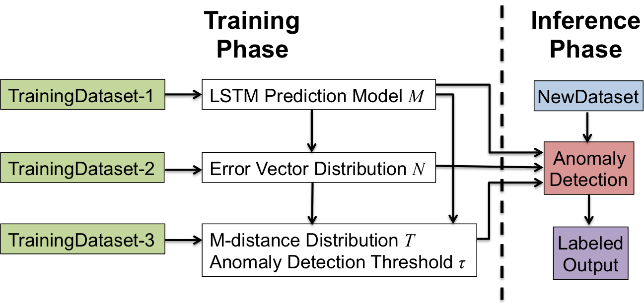
Figure 1. Training and Inference Phases in Greenhouse

Training Phase: Training is performed in four key steps:

1. Split a non-anomalous dataset into three: TrainingDataset-1, TrainingDataset-2, TrainingDataset-3.

2. Train an LSTM prediction model $M$ with TrainingDataset-1.

3. Apply $M$ over TrainingDataset-2 to make predictions and compute error vectors. Then fit the resulting error vectors into a multi-variate normal distribution $N$.

4. Apply $M$ over TrainingDataset-3 to make predictions and compute error vectors. Then compute M-distances (Mahalanobis-distances (Mahalanobis, 1936)), and fit the resulting M-distances into a truncated normal distribution $T$. Finally, evaluate the inverse cumulative distribution function of $T$ at a user-specified percentile to be used as the anomaly detection threshold $\tau$.

Inference Phase: Inference involves the following steps:

1. Apply $M$ over NewDataset to make predictions.

2. Compute error vectors.

3. Compute M-distances between these error vectors and the center of $N$.

4. Finally, label the time-series values whose M-distances exceed $\tau$ as anomalies.

Table 2. Greenhouse vs. LSTM-AD (Malhotra et al., 2015)

	Precision	Recall	$F_{1}$ score
Greenhouse (Twitter_AAPL)	0.49	0.06	0.11
LSTM-AD (Twitter_AAPL)	0.22	0.14	0.17
Greenhouse (nyc_taxi)	0.25	0.58	0.35
LSTM-AD (nyc_taxi)	0.26	0.82	0.40

We implemented this algorithm on top of TensorFlow (Abadi et al., 2016), and compared its anomaly detection accuracy with LSTM-AD (Malhotra et al., 2015), based on real-world datasets from the Numenta Anomaly Benchmark (Lavin and Ahmad, 2015). LSTM-AD fundamentally differs from Greenhouse in that, it is not zero-positive, i.e., it requires anomalous samples to be present in its training datasets. We present a sample experimental result in Table 2. For two different datasets, Greenhouse performed favorably over LSTM-AD in terms of its Precision and managed to maintain a close $F_{1}$ score, despite its lower Recall. This is a remarkable result, especially given that Greenhouse uses significantly smaller training data (about 25% and 55% that of LSTM-AD, respectively) and does not rely on any anomalous samples. We believe these are powerful qualities, making Greenhouse more generally applicable in practice.

3. Ongoing Research

Going forward, we are working on a number of research issues to extend our algorithmic framework into a full-feature time-series anomaly detection system for IoT. We conclude the paper with an overview of these issues.

Training dataset management: In Greenhouse, we use multiple datasets during training. Furthermore, for sequential data like time-series, respecting order, regularity (isochronism), and continuity is important in correctly capturing patterns of interest. In order to avoid the risk of over/under-fitting and to preserve continuity, we need to pay attention to how we choose and arrange our training datasets.

Range-based anomalies and their evaluation: Time-series anomalies often manifest themselves over a period of time rather than at single time points (so-called range-based or collective anomalies (Chandola et al., 2009; Bontemps et al., 2017)). Furthermore, judging accuracy of results in this context is highly intricate and application-dependent. We are extending Greenhouse with models and algorithms to handle range-based anomalies in a principled manner (Lee et al., 2018).

Real-time anomaly detection: Our algorithmic framework initially focused on operating in an “offline mode”, where both training and inference are applied on finite datasets that have been collected in the past and are being analyzed retrospectively after the fact. In many IoT applications, real-time anomaly detection on live data is also important. Thus, we are extending Greenhouse to operate in an “online mode”, which requires continuous, low-latency inferencing (and possibly training) over streaming time-series. This includes things like carefully analyzing the impact of algorithm and model parameters on accuracy and performance, and properly tuning them as datasets change.

Utilizing human feedback: When deployed in an online setting, Greenhouse will start making anomaly predictions on new datasets as well as potentially saving these (self-labeled) datasets for further training. Furthermore, feedback from human may be available to validate anomaly predictions or to course-correct. We plan to augment Greenhouse with reinforcement learning techniques to utilize such feedback when available (Bakker, 2001).

Data management support: As in any deep learning system, data is an indispensable resource in Greenhouse. We will deploy Greenhouse and study its data management needs within the context of a time-series data management system environment (e.g., Metronome (Meehan et al., 2017)). This includes things like providing methods of efficient and consistent access to arbitrary windows of data needed by Greenhouse algorithms.

Exploiting high-performance compute frameworks: While implemented on top of a state-of-the-art machine learning framework (Abadi et al., 2016), Greenhouse does not yet take full advantage of high-performance compute facilities provided by such frameworks. We plan to extend Greenhouse in this direction, including exploring its use in conjunction with other complementary tools and libraries, such as Intel^® Nervana^™ Graph (Intel, 2017).

Support for distributed IoT deployments: IoT applications typically execute on multi-tier deployments from wireless networks of edge devices to more powerful cloud servers. We plan to investigate the use of Greenhouse in such distributed deployments with heterogeneous computing resources.

Acknowledgments. This research has been funded in part by Intel.

References

- (1)
- Abadi et al. (2016) Martin Abadi, Paul Barham, Jianmin Chen, Zhifeng Chen, Andy Davis, Jeffrey Dean, Matthieu Devin, Sanjay Ghemawat, Geoffrey Irving, Michael Isard, Manjunath Kudlur, Josh Levenberg, Rajat Monga, Sherry Moore, Derek G. Murray, Benoit Steiner, Paul Tucker, Vijay Vasudevan, Pete Warden, Martin Wicke, Yuan Yu, and Xiaoqiang Zheng. 2016. TensorFlow: A System for Large-scale Machine Learning. In 12th USENIX Symposium on Operating Systems Design and Implementation (OSDI). 265–283.
- Aggarwal (2013) Charu C. Aggarwal. 2013. Outlier Analysis. Springer.
- Alam et al. (2017) Mohammad Mejbah Ul Alam, Justin Gottschlich, and Abdullah Muzahid. 2017. AutoPerf: A Generalized Zero-Positive Learning System to Detect Software Performance Anomalies. Technical Report. http://arxiv.org/abs/1709.07536/
- Bailis et al. (2017) Peter Bailis, Edward Gan, Samuel Madden, Deepak Narayanan, Kexin Rong, and Sahaana Suri. 2017. MacroBase: Prioritizing Attention in Fast Data. In ACM International Conference on Management of Data (SIGMOD). 541–556.
- Bakker (2001) Bram Bakker. 2001. Reinforcement Learning with Long Short-term Memory. In 14th International Conference on Neural Information Processing Systems (NIPS). 1475–1482.
- Bontemps et al. (2017) Loic Bontemps, Van Loi Cao, James McDermott, and Nhien-An Le-Khac. 2017. Collective Anomaly Detection based on Long Short Term Memory Recurrent Neural Network. Technical Report. https://arxiv.org/abs/1703.09752
- Chandola et al. (2009) Varun Chandola, Arindam Banerjee, and Vipin Kumar. 2009. Anomaly Detection: A Survey. ACM Computing Surveys 41, 3 (2009), 15:1–15:58.
- Christopher Olah (2015) Christopher Olah. 2015. Understanding LSTM Networks. http://colah.github.io/posts/2015-08-Understanding-LSTMs/. (2015).
- Hochreiter and Schmidhuber (1997) Sepp Hochreiter and Jurgen Schmidhuber. 1997. Long Short-Term Memory. Neural Computation 9, 8 (1997), 1735–1780.
- Intel (2017) Intel. 2017. Intel Nervana Graph. http://ngraph.nervanasys.com/. (2017).
- Lavin and Ahmad (2015) Alexander Lavin and Subutai Ahmad. 2015. Evaluating Real-Time Anomaly Detection Algorithms - The Numenta Anomaly Benchmark. In 14th IEEE International Conference on Machine Learning and Applications (ICMLA). 38–44.
- Lee et al. (2018) Tae Jun Lee, Justin Gottschlich, Nesime Tatbul, Eric Metcalf, and Stan Zdonik. 2018. Precision and Recall for Range-Based Anomaly Detection. https://arxiv.org/abs/1801.03175/. In SysML Conference.
- Mahalanobis (1936) Prasanta Chandra Mahalanobis. 1936. On the Generalised Distance in Statistics. Proceedings of the National Institute of Sciences of India 2, 1 (1936), 49–55.
- Malhotra et al. (2015) Pankaj Malhotra, Lovekesh Vig, Gautam Shroff, and Puneet Agarwal. 2015. Long Short Term Memory Networks for Anomaly Detection in Time Series. In European Symposium on Artificial Neural Networks, Computational Intelligence and Machine Learning (ESANN). 89–94.
- Meehan et al. (2017) John Meehan, Cansu Aslantas, Stan Zdonik, Nesime Tatbul, and Jiang Du. 2017. Data Ingestion for the Connected World. In Conference on Innovative Data Systems Research (CIDR).