$\mathcal{NP}$-Completeness and Inapproximability of the
Virtual Network Embedding Problem and Its Variants

Abstract

Many resource allocation problems in the cloud can be described as a basic Virtual Network Embedding Problem (VNEP): the problem of finding a mapping of a request graph (describing a workload) onto a substrate graph (describing the physical infrastructure). Applications range from mapping testbeds (from where the problem originated), over the embedding of batch-processing workloads (virtual clusters) to the embedding of service function chains. The different applications come with their own specific requirements and constraints, including node mapping constraints, routing policies, and latency constraints. While the VNEP has been studied intensively over the last years, complexity results are only known for specific models and we lack a comprehensive understanding of its hardness.

This paper charts the complexity landscape of the VNEP by providing a systematic analysis of the hardness of a wide range of VNEP variants, using a unifying and rigorous proof framework. In particular, we show that the problem of finding a feasible embedding is $\mathcal{NP}\text{-complete}$ in general, and, hence, the VNEP cannot be approximated under any objective, unless $\mathcal{P}{\,=\,}\mathcal{NP}$ holds. Importantly, we derive $\mathcal{NP}\text{-completeness}$ results also for finding approximate embeddings, which may violate, e.g., capacity constraints by certain factors. Lastly, we prove that our results still pertain when restricting the request graphs to planar or degree-bounded graphs.

I Introduction

At the heart of the cloud computing paradigm lies the idea of efficient resource sharing: due to virtualization, multiple workloads can co-habit and use a given resource infrastructure simultaneously. Indeed, cloud computing introduces great flexibilities in terms of where workloads can be mapped. At the same time, exploiting this mapping flexibility poses a fundamental algorithmic challenge. In particular, in order to provide predictable performance, guarantees on all, i.e. node and edge, resources need to be ensured. Indeed, it has been shown that cloud application performance can suffer significantly from interference on the communication network [talkabout].

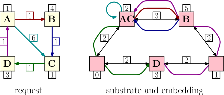
The underlying algorithmic problem is essentially a graph theoretical one: both the workload as well as the infrastructure can be modeled as graphs. The former, the so-called request graph, describes the resource requirements both on the nodes (e.g., the virtual machines) as well as on the interconnecting network. The latter, the so-called substrate graph, describes the physical infrastructure and its resources (servers and links). Figure 1 depicts an example of embedding a request graph.

The problem is known in the networking community under the name Virtual Network Embedding Problem (VNEP) and has been studied intensively for over a decade [vnep, vnep-survey]. Besides the rather general study of the VNEP, which emerged originally from the study of testbed provisioning, essentially the same problems are considered in the context of Service Function Chaining [mehraghdam2014specifying, rfc7665], as well as in the context of embeddings Virtual Clusters, a specific batch processing request abstraction [ballani2011towards, ccr15emb].

Figure 1: Example of embedding a request (left) on a substrate network (right). The numeric labels at the network elements denote the demanded resources and the available capacity, respectively. In the embedding, request nodes A and C are collocated on the same substrate node, such that the request edge $(\textnormal{{A}},\textnormal{{C}})$ does not use any substrate edge resources.

TABLE I: Overview on results obtained in this paper.

			VNEP variants	Identifier according to Definition 8	$\langle$ VE $|$ - $\rangle$	$\langle$ E $|$ N $\rangle$	$\langle$ V $|$ R $\rangle$	$\langle$ - $|$ NR $\rangle$	$\langle$ - $|$ NL $\rangle$
				Enforcing Node Capacities	✓	$\star$	✓	$\star$	$\star$
				Enforcing Edge Capacities	✓	✓	$\star$	$\star$	$\star$
				Enforcing Node Placement Restrictions	$\star$	✓	$\star$	✓	✓
				Enforcing Edge Routing Restrictions	$\star$	$\star$	✓	✓	$\star$
				Enforcing Latency Restrictions	$\star$	$\star$	$\star$	$\star$	✓
Results	Section LABEL:sec:np-completeness-of-the-vnep	$\mathcal{NP}$-completeness and inapproximability under any objective			Thm. LABEL:thm:vnep-capacity-nodes-and-edges-is-np-complete	Thm. LABEL:thm:decision-edge-capacities-node-placement	Thm. LABEL:thm:node-capacities-routing-restrictions	Thm. LABEL:thm:without-capacities-node-placement-and-routing-or-latencies	Thm. LABEL:thm:without-capacities-node-placement-and-routing-or-latencies
	Section LABEL:sec:np-completeness-approximate-embeddings	$\mathcal{NP}\text{-completeness}$ and inapproximability when increasing node capacities by a factor $\alpha<2$			Thm. LABEL:thm:alpha-approximate-embeddings	-	Thm. LABEL:thm:alpha-approximate-embeddings	-	-
		Inapproximability when increasing edge capacities by a factor $\beta\in\Theta(\log n/\log\log n)$ (unless $\mathcal{NP}\subseteq\mathcal{BP}\text{-}\textit{TIME}(\bigcup_{d\geq 1}n^{d\log\log n})$)			Thm. LABEL:thm:beta-inapproximability	Thm. LABEL:thm:beta-inapproximability	-	-	-
		$\mathcal{NP}\text{-completeness}$ and inapproximability when loosening latency bounds by a factor $\gamma<2$			-	-	-	-	Thm. LABEL:thm:gamma-approximate-embeddings
	Section LABEL:sec:np-completeness-graph-restrictions	Results are preserved for acyclic substrates (except for Thm. LABEL:thm:beta-inapproximability)			Obs. LABEL:obs:vnep-on-dags
		Results are preserved for acyclic, planar, degree-bounded requests			Thm. LABEL:thm:np-completeness-on-restricted-request-graphs

I-A Related Work

Objectives & Restrictions

Depending on the setting, many different objectives are considered for the VNEP. The most studied ones concern minimizing the (resource allocation) cost [vnep, vnep-survey], maximizing the profit by exerting admission control [even2013competitive, rostSchmidFeldmann2014], and minimizing the maximal load [mehraghdam2014specifying, chowdhury2012vineyard].

Besides commonly enforcing that the substrate’s physical capacities on servers and edges are not exceeded to provide Quality-of-Service [vnep-survey], additional restrictions have emerged:

• Restrictions on the placement of virtual nodes first arose to enforce closeness to locations of interest [vnep], but were also used in the context of privacy policies to restrict mappings to certain countries [schaffrath2012optimizing]. However, these restrictions are now also used in the context of Service Function Chaining, as specific functions may only be mapped on x86 servers, while firewall appliances cannot [mehraghdam2014specifying, rfc7665].

• Routing restrictions first arose in the context of expressing security policies, as for example some traffic may not be routed via insecure domains or physical links shall not be shared with other virtual networks [vnep-survey, bays2012security].

• Restrictions on latencies were studied for the VNEP in [infuhr2011introducing] and have been recently studied intensely in the context of Service Function Chaining to achieve responsiveness and Quality-of-Service [mehraghdam2014specifying, rfc7665].

Algorithmic Approaches

Several dozens of algorithms were proposed to solve the VNEP and its siblings, including the Virtual Cluster Embedding [ballani2011towards] and Service Function Chain Embedding problem [vnep-survey]. Most approaches to solve the VNEP either rely on heuristics [vnep] or metaheuristics [vnep-survey]. On the other hand, several works study exact (non-polynomial time) algorithms to solve the problem to (near-)optimality or to devise heuristics. Mixed Integer Programming is the most widely used exact approach [mehraghdam2014specifying, rostSchmidFeldmann2014, infuhr2011introducing].

Only recently, approximation algorithms providing quality guarantees for the VNEP have been presented. In particular, the embedding of chains is approximated under assumptions on the requested resources and the achievable benefit in [sirocco16path]. In [rostSchmidLeveragingRRIFIPwithPreprint] approximations for cactus request graphs are detailed, while [rostSchmidFPTApproximations] presents fixed-parameter tractable approximations for arbitrary request graph topologies.

Complexity Results

Surprisingly, despite the relevance of the problem and the large body of literature, the complexity of the underlying problems has not received much attention. While it can be easily seen that the Virtual Network Embedding Problem encompasses several $\mathcal{NP}$-hard problems as e.g. the $k$-disjoint paths problem [chuzhoy2007hardness], the minimum linear arrangment problem [mla-survey], or the subgraph isomorphism problem [eppstein1995subgraph], most works on the VNEP cite a $\mathcal{NP}\text{-hardness}$ result contained in a technical report from 2002 by Andersen [andersen2002theoretical]. The only other work studying the computational complexity is one by Amaldi et al. [amaldi2016computational], which proved the $\mathcal{NP}\text{-hardness}$ and inapproximability of the profit maximization objective while not taking into account latency or routing restrictions and not considering the hardness of embedding a single request.

I-B Contributions and Overview

In this work, we initiate the systematic study of the computational complexity of the VNEP. Taking all the aforementioned restrictions into account, we first compile a concise taxonomy of the VNEP variants in Section II. Then, we present a powerful reduction framework in Section LABEL:sec:reduction-framework, which is the base for nearly all hardness results presented in this paper. In particular, we show the following (see also Table I):

• We show the $\mathcal{NP}\text{-completeness}$ of five different VNEP variants in Section LABEL:sec:np-completeness-of-the-vnep. For example, we consider the variant only enforcing capacity constraints, but also one in which only node placement and latency restrictions must be obeyed in the absence of capacity constraints.

• We extend these results in Section LABEL:sec:np-completeness-approximate-embeddings and show that the considered variants remain $\mathcal{NP}\text{-complete}$ even when computing approximate embeddings, which may exceed latency or capacity constraints by certain factors.

• Lastly, we show in Section LABEL:sec:np-completeness-graph-restrictions that the respective VNEP variants remain $\mathcal{NP}\text{-complete}$ even when restricting substrate graphs to directed acyclic graphs (DAGs) and request graphs to planar, degree-bounded DAGs.

As we are proving $\mathcal{NP}\text{-completeness}$ throughout this paper, the implications of our results are severe. Given the $\mathcal{NP}\text{-completeness}$ of finding any feasible solution, finding an optimal solution subject to any objective is at least $\mathcal{NP}\text{-hard}$. Furthermore, unless $\mathcal{P}{\,=\,}\mathcal{NP}$ holds, the respective variants cannot be approximated to within any factor.

Table I summarizes our results and is to be read as follows. Any of the five rightmost columns represents a specific VNEP variant. The $\checkmark$ symbol indicates restrictions that are enforced, while the $\star$ symbol indicates restrictions which are not considered. Importantly, enabling a $\star$ restriction, does not change the results (cf. Lemma 9). Considering a specific variant, the respective column should be read from top to bottom. For example, for $\langle$ VE $|$ - $\rangle$, its $\mathcal{NP}\text{-completeness}$ is shown in Theorem LABEL:thm:vnep-capacity-nodes-and-edges-is-np-complete while its inapproximability when relaxing edge capacity constraints is shown in Theorem LABEL:thm:beta-inapproximability. Lastly, all results also hold under the graph restrictions of the two bottom rows.

II Formal Model

Within this section we formalize the VNEP, introduce its variants, and lastly provide an Integer Programming formulation to solve any of the variants.

Notation

The following notation is used throughout this work. We use $[x]$ to denote $\{1,2,\ldots,x\}$ for $x\in\mathbb{N}$. For a directed graph $G=(V,E)$, we denote by $\delta^{+}(v)\subseteq E$ and $\delta^{-}(v)\subseteq E$ the outgoing and incoming edges of node $v\in V$. When considering functions on tuples, we omit the parantheses of the tuple and simply write $f(a,b)$ instead of $f((a,b))$.

II-A Basic Problem Definition

We refer to the physical network as substrate network and model it as directed graph $G_{S}=(V_{S},E_{S})$. Capacities in the substrate are given by the function $c_{S}:V_{S}\cup E_{S}\to\mathbb{R}_{\geq 0}\cup\{\infty\}$. The capacity $c_{S}(u)$ of node $u\in V_{S}$ may represent for example the number of CPUs while the capacity $c_{S}(u,v)$ of edge $(u,v)\in E_{S}$ represents the available bandwidth. By allowing to set substrate capacities to $\infty$, the capacity constraints on the respective substrate elements can be effectively disabled. We denote by $\mathcal{P}_{S}$ the set of all simple paths in $G_{S}$.

A request is similarly modeled as directed graph $G_{r}=(V_{r},E_{r})$ together with node and edge capacities (demands) $c_{r}:V_{r}\cup E_{r}\to\mathbb{R}_{\geq 0}$.

The task is to find a mapping of request graph $G_{r}$ on the substrate network $G_{S}$, i.e. a mapping of request nodes to substrate nodes and a mapping of request edges to paths in the substrate. Virtual nodes and edges can only be mapped on substrate nodes and edges of sufficient capacity. Accordingly, we denote by $V^{{i}}_{S}=\{u\in V_{S}|c_{S}(u)\geq c_{r}(i)\}$ the set of substrate nodes supporting the mapping of node $i\in V_{r}$ and by $E^{{i,j}}_{S}=\{(u,v)\in E_{S}|c_{S}(u,v)\geq c_{r}(i,j)\}$ the substrate edges supporting the mapping of virtual edge $(i,j)\in E_{r}$.

Definition 1 (Valid Mapping).

A valid mapping of request $G_{r}$ to the substrate $G_{S}$ is a tuple $m=(m_{V},m_{E})$ of functions that map nodes and edges, respectively, s.t. the following holds:

• The function $m_{V}:V_{r}\to V_{S}$ maps virtual nodes to suitable substrate nodes, such that $m_{V}(i)\in V^{{i}}_{S}$ holds for $i\in V_{r}$.

• The function $m_{E}:E_{r}\to\mathcal{P}_{S}$ maps virtual edges $(i,j)\in E_{r}$ to simple paths in $G_{S}$ connecting $m_{V}(i)$ to $m_{V}(j)$, such that $m_{E}(i,j)\subseteq E^{{i,j}}_{S}$ holds for $(i,j)\in E_{r}$.

∎

Considering the above definition, note the following. Firstly, the mapping $m_{E}(i,j)$ of the virtual edge $(i,j)\in E_{r}$ may be empty, if (and only if) $i$ and $j$ are mapped on the same substrate node. Secondly, the definition only enforces that single resource allocations do not exceed the available capacity. To enforce that the cumulative allocations respect capacities, we introduce the following:

Definition 2 (Allocations).

We denote by $A_{m}(x)\in\mathbb{R}_{\geq 0}$ the resource allocations induced by valid mapping $m=(m_{V},m_{E})$ on substrate element $x\in G_{S}$ and define

$$\huge A_{m}(u) = \textstyle\sum_{i\in V_{r}:m_{V}(i)=u}c_{r}(i)$$

$$A_{m}(u,v) = \textstyle\sum_{(i,j)\in E_{r}:(u,v)\in m_{E}(i,j)}c_{r}(i,j)$$

for node $u\in V_{S}$ and edge $(u,v)\in E_{S}$, respectively. ∎

We call a mapping feasible, if the (cumulative) allocations do not exceed the capacity of any substrate element:

Definition 3 (Feasible Embedding).

A mapping $m$ is a feasible embedding, if the allocations do not exceed the capacity, i.e. $A_{m}(x)\leq c_{S}(x)$ holds for $x\in G_{S}$. ∎

In this paper we study the decision variant of the VNEP, asking whether there exists a feasible embedding:

Definition 4 (VNEP, Decision Variant).

Given is a single request $G_{r}$ that shall be embedded on the substrate graph $G_{S}$. The task is to find any feasible embedding or to decide that no feasible embedding exists. ∎

II-B Variants of the VNEP & Nomenclature

As discussed when reviewing the related work in Section I-A, additional requirements are enforced in many settings. Accordingly, we now formalize (i) node placement, (ii) edge routing, and (iii) latency restrictions. Node placement and edge routing restrictions effectively exclude potential mapping options for nodes and edges. For latency restrictions we introduce latency bounds for each of the virtual edges.

Definition 5 (Node Placement Restrictions).

For each virtual node $i\in V_{r}$ a set of forbidden substrate nodes $\overline{V}^{{i}}_{S}\subset V_{S}$ is provided. Accordingly, the set of allowed nodes $V^{{i}}_{S}$ is defined to be $\{u\in V_{S}\setminus\overline{V}^{{i}}_{S}\,|\,c_{S}(u)\geq c_{r}(i)\}$. ∎

Definition 6 (Routing Restrictions).

For each virtual edge $(i,j)\in E_{r}$ a set of forbidden substrate edges $\overline{E}^{{i,j}}_{S}\subseteq E_{S}$ is provided. Accordingly, the set of allowed edges $E^{{i,j}}_{S}$ is set to be $\{(u,v)\in E_{S}\setminus\overline{E}^{{i,j}}_{S}\,|\,c_{S}(u,v)\geq c_{r}(i,j)\}$. ∎

Definition 7 (Latency Restrictions).

For each substrate edge $e\in E_{S}$ the edge’s latency is given via $l_{S}(e)\in\mathbb{R}_{\geq 0}$. Latency bounds for virtual edges are specified via the function $l_{r}:E_{r}\to\mathbb{R}_{\geq 0}\cup\{\infty\}$, such that the latency along the substrate path $m_{E}(i,j)$, used to realize the edge $(i,j)\in E_{r}$, is less than $l_{r}(i,j)$. Formally, the definition of feasible embeddings (cf. Definition 3) is extended by including that $\sum_{e\in m_{E}(i,j)}l_{S}(e)\leq l_{r}(i,j)$ holds for $(i,j)\in E_{r}$. ∎

We introduce the following taxonomy to denote the different problem variants.

Definition 8 (Taxonomy).

We use the notation $\langle$ C $|$ A $\rangle$ to indicate whether and which of the capacity constraints C and which of the additional constraints A are enforced.

C

We denote by V node capacities, by E edge capacities, and by - that none are used. When node or edge capacities are not considered, we set the capacities of the respective substrate elements to $\infty$.

A

For the additional restrictions -, N, L, and R stand for no restrictions, node placement, latency, and routing restrictions, respectively.

∎

Hence, $\langle$ VE $|$ - $\rangle$ indicates the classic VNEP without additional constraints while obeying capacities and $\langle$ - $|$ NL $\rangle$ indicates the combination of node placement and latency restrictions without considering substrate capacities. We note that the introduction of more restrictions only makes the respective problem harder:

Lemma 9.

A VNEP variant $\langle$ A $|$ C $\rangle$ that encompasses all restrictions of $\langle$ A’ $|$ C’ $\rangle$ is at least as hard as $\langle$ A’ $|$ C’ $\rangle$.

Proof.

The capacity constraints as well as the additional requirements were all formulated in such a fashion that any one of these can be disabled. Considering capacities and latencies, one may set the respective substrate capacities to $\infty$ and the latencies of edges to $0$, respectively. For node placement and edge restrictions one may set the forbidden node and edge sets to the empty set. Hence, there exists a trivial reduction from $\langle$ A $|$ C $\rangle$ to $\langle$ A’ $|$ C’ $\rangle$ and the result follows. ∎

II-C Relaxing Constraints

Within this work, we show the VNEP to be $\mathcal{NP}\text{-complete}$ under many meaningful restriction combinations. This in turn also implies the inapproximability of the respective VNEP variants (unless $\mathcal{P}{\,=\,}\mathcal{NP}$). Hence, it is natural to consider a broader class of (approximation) algorithms that may violate constraints by a certain factor: instead of answering the question whether a valid embedding exists that satisfies all capacity constraints, one might for example seek an embedding that uses at most two times the actual capacities. We refer to these embeddings as approximate embeddings:

Definition 10 ($\alpha$- / $\beta$- / $\gamma$-Approximate Embeddings).

A mapping $m$ is an approximate embedding, if it is valid and violates capacity or latency constraints only within a certain bound. Specifically, we call an embedding $\alpha$- and $\beta$-approximate, when node and edge allocations are bounded by $\alpha$ and $\beta$ times the respective node or edge capacity. Considering latency restrictions, we call a mapping $\gamma$-approximate when latencies are within a factor of $\gamma$ of the original bound. Formally, the following must hold for $\alpha,\beta,\gamma\geq 1$:

$$A_{m}(u) \,\leq\, \alpha\cdot c_{S}(u) \forall u\in V_{S}$$

$$A_{m}(u,v) \leq \beta\cdot c_{S}(u,v)\quad \forall(u,v)\in E_{S}$$

$$\sum_{e\in m_{E}(i,j)}l_{S}(e) \leq \gamma\cdot l_{r}(i,j) \forall(i,j)\in E_{r} \square$$

II-D Integer Programming Formulation

We now give an Integer Programming (IP) formulation, which can be used to solve any of the considered decision VNEP variants. A similar formulation was proposed in [infuhr2011introducing]. Given the hardness results presented in this paper and given that solving IPs lies in $\mathcal{NP}$ [papadimitriou1981complexity], the IP may serve as an attractive approach to solve the respective variants in exponential time. Besides the practical application, the existence of our formulation (constructively) shows that the VNEP variants considered here are also all contained in $\mathcal{NP}$.

Our formulation naturally encompasses node placement and routing restrictions, while for latencies an additional constraint is introduced. The decision variable $x\in\{0,1\}$ is used to indicate, whether the request graph $G_{r}$ is embedded or not. By maximizing $x$, the IP decides whether a feasible embedding exists ($x=1$) or whether no such embedding exists ($x=0$). The mapping of virtual nodes is modeled using decision variables $y^{u}_{i}\in\{0,1\}$ for $i\in V_{r}$ and $u\in V_{S}$. If $y^{u}_{i}=1$ holds, then the virtual node $i\in V_{r}$ is mapped on substrate node $u\in V_{S}$. Constraint II-D enforces that each virtual node is mapped to one substrate node, if the request is embedded $(x=1)$, while Constraint II-D excludes unsuitable substrate nodes.

For computing edge mappings the decision variables $z^{u,v}_{i,j}\in\{0,1\}$ for $(i,j)\in E_{r}$ and $(u,v)\in E_{S}$ are employed. If $z^{u,v}_{i,j}=1$ holds, then the substrate edge $(u,v)$ lies on the path $m_{E}(i,j)$. Constraints II-D and II-D embed virtual links as paths in the substrate, if the request is embedded. In particular, Constraint II-D constructs a unit flow for virtual edge $(i,j)\in E_{r}$ from the location $u\in V_{S}$ onto which $i$ was mapped ($y^{u}_{i}=1$) to the location $v\in V_{S}$ onto which $j$ was mapped ($y^{v}_{j}=1$), while Constraint II-D excludes unsuitable edges. Constraints II-D and LABEL:alg:ip:edge-capacity enforce that substrate capacities are obeyed. Lastly, Constraint LABEL:alg:ip:latency is only used when latencies are considered: it enforces that the sum of latencies along the embedding path of a virtual edge is smaller than the respective latency bound.

	(1)
$$

∑u∈VSyui $\displaystyle=$ $\displaystyle x$ $\displaystyle\forall i\in V_{r}$  (2) $$

∑u∈VS∖ViSyui $\displaystyle=$ $\displaystyle 0$ $\displaystyle\forall i\in V_{r}$  (3) $$

∑(u,v)∈δ+(u)zu,vi,j-∑(v,u)∈δ-(u)zv,ui,j $\displaystyle=$ $\displaystyle y^{u}_{i}-y^{u}_{j}{}{}$ $\displaystyle\forall(i,j)\in E_{r},u\in E_{S}$  (4) $$

∑(u,v)∈ES∖Ei,jSzu,vi,j $\displaystyle=$ $\displaystyle 0$ $\displaystyle\forall(i,j)\in E_{r}$  (5) $$

∑i∈Vrcr(i)⋅yui $\displaystyle\leq$ $\displaystyle c_{S}(u)$ $\displaystyle\forall u\in V_{S}$  (6) $$

∑(i,j)∈Ercr(i,