Recognizing Material Properties from Images

Abstract

Humans implicitly rely on properties of the materials that make up ordinary objects to guide our interactions. Grasping smooth materials, for example, requires more care than rough ones, and softness is an ideal property for fabric used in bedding. Even when these properties are not purely visual (softness is a physical property of the material), we may still infer the softness of a fabric by looking at it. We refer to these visually-recognizable material properties as visual material attributes. Recognizing visual material attributes in images can contribute valuable information for general scene understanding and for recognition of materials themselves. Unlike well-known object and scene attributes, visual material attributes are local properties. “Fuzziness”, for example, does not have a particular shape. We show that given a set of images annotated with known material attributes, we may accurately recognize the attributes from purely local information (small image patches). Obtaining such annotations in a consistent fashion at scale, however, is challenging. We introduce a method that allows us to solve this problem by probing the human visual perception of materials to automatically discover unnamed attributes that serve the same purpose. By asking simple yes/no questions comparing pairs of image patches, we obtain sufficient weak supervision to build a set of attributes (and associated classifiers) that, while being unnamed, serve the same function as the named attributes, such as “fuzzy” or “rough”, with which we describe materials. Doing so allows us to recognize visual material attributes without resorting to exhaustive manual annotation of a fixed set of named attributes. Furthermore, we show that our automatic attribute discovery method may be integrated in the end-to-end learning of a material classification CNN framework to simultaneously recognize materials and discover their visual material attributes. Our experimental results show that visual material attributes, whether named or automatically discovered, provide a useful intermediate representation for known material categories themselves as well as a basis for transfer learning when recognizing previously-unseen categories.

1 Introduction

Properties of the materials that appear in everyday scenes inform many of the decisions we make when interacting with things made from these materials. When cleaning a glass cup, for example, we know not to drop it or it will break. Glass is also often smooth, and we grasp it accordingly so it will not slip. Examples of material properties include visual properties, such as glossiness or translucency, as well as physical or tactile properties, such as hardness or roughness. We can see the presence of these material properties simply by looking at ordinary images, suggesting that even non-visual properties can be inferred from the visual appearance of the material. We refer to such visually-recognizable material properties as visual material attributes. Recognizing these visual material attributes in images would allow us to better understand and interact with the scenes in which materials appear.

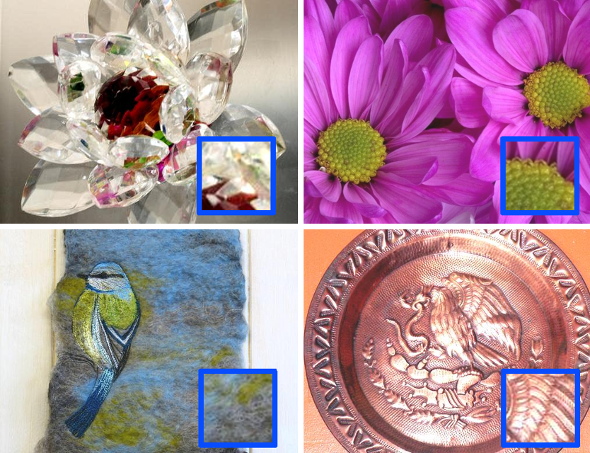
Figure 1: Materials are unique in that they have many characteristic locally-recognizable visual attributes. Wool, for example, often appears “fuzzy”, and metals are typically “shiny”. In this work we show that material attributes can be recognized from purely local information, that we can discover these visual attributes automatically (again from purely local information), and that such a process can be applied to large-scale material image datasets via an end-to-end formulation in a Convolutional Neural Network.

Recognizing visual material attributes in images, however, is particularly challenging. Unlike much prior work in object, face, and scene attribute recognition [1, 2, 3, 4], material attributes are local properties, as can be seen in Figure 1. While scene, object, and face attributes are typically associated with a characteristic shape and fixed spatial extent, material attributes are not. A car that is “sporty” will have a typically sleek and aerodynamic shape, and if a face has “large eyes”, such an attribute is defined by the spatial extent of the eyes relative to the face. If a carpet is “fuzzy”, however, the fuzziness is not associated with any characteristic shape or scale, nor is it necessarily a consequence of the object involved (some carpets are not fuzzy).

In a preliminary experiment, we show that given a fully-supervised dataset containing material annotations, a set of named semantic material attributes (such as “fuzzy”, “organic”, or “transparent”), and sparse per-pixel labels for these attributes, we can indeed recognize visual material properties from small local image patches. Such a method can be applied in a sliding window fashion to produce per-pixel predictions for material attributes in arbitrary images. The accuracy of these predictions supports our claim that material attributes are indeed locally-recognizable and can be recognized at the per-pixel level. Furthermore, we show that these attributes alone can be used to recognize materials in a way that separates the material itself from the surrounding context such as objects and scenes.

The primary drawback of a straightforward fully-supervised approach, such as the one described above, is that it requires a set of consistent annotations for the material attributes. Some material attributes are intuitive and challenging to precisely define. If we wish to scale the annotation process to multiple annotators, we can no longer assume that a single person is providing attribute labels in a consistent and complete fashion. Additionally, such a method implicitly depends on the choice of a fixed set of named material attributes. This restriction gives us no way of evaluating if the chosen set of material attributes is complete or if there are possibly more attributes that we may implicitly associate with materials.

Rather than assuming that we can exhaustively describe the set of attributes humans associate with materials, we show that we can instead directly probe the human visual perception of materials using simple yes/no questions. Using the answers to these questions as a form of weak supervision, we derive a method for discovering a set of unnamed locally-recognizable visual material attributes that faithfully encodes our own human perceptual representation of materials. Our method requires only material annotations, and discovers unnamed attributes with the same desirable properties as the fixed named material attributes we described previously, while using only a small amount of easily-collected weak supervision.

Our attribute discovery method requires only simple supervision and eliminates the need to manually define a set of named material attributes for full supervision. The training process is, however, still not ideal for application to modern large-scale image databases. Working well with small amounts of training data is a benefit, but we would ideally like to leverage recent advances in large-scale end-to-end learning as well. To this end, we show that the same material attributes can in fact be discovered within a Convolutional Neural Network (CNN) framework focused on material recognition in local image patches (the Material Attribute/Category CNN, MAC-CNN). This enables us to take advantage of potentially larger material datasets. We also find interesting parallels with the material representation in the human material recognition process as observed in neuroscience [5, 6]. In contrast to the intermediate representations formed by previous attribute methods, the human material recognition process (and our MAC-CNN) produces a perceptual representation, i.e. visual material attributes, as a side-product of material category recognition. Our results show that we are able to discover similar perceptual attributes using the MAC-CNN, and we additionally demonstrate the usefulness of perceptual material attributes for transfer learning.

2 Related Work

In this paper we discuss the recognition of material properties from images. There is much recent work in the areas of attribute recognition, material recognition, and human visual perception that is relevant to our work; we discuss these findings below.

2.1 Attributes

2.1.1 Fully-Supervised Attributes

Fully-supervised visual attributes have been widely used in object and scene recognition, but largely at the image or scene level. Ferrari and Zisserman [2] introduced a generative model for certain pattern and color attributes, such as “dots”, or “stripes”. The attributes described in their model focus on texture and color, but are not material attributes. A paper cup, for example, may have stripes painted on it, but “striped” is not a property of the paper itself; it is in fact a property of the cup. Kumar et al. [3] proposed a face search engine with their attribute-based FaceTracer framework. FaceTracer uses SVM and AdaBoost to recognize attributes within fixed facial regions. Such fixed regions are not present in materials, which may take on an arbitrary shape unlike the objects which they make up. Farhadi et al. [1] applied attributes to the problem of object recognition. Their results showed an improvement in accuracy over a basic approach using texture features. Lampert et al. [7] also showed that attributes transfer information between disjoint sets of classes. These results suggest that attributes can serve as an intermediate representation for recognition of the categories which exhibit them. Patterson and Hays [4] showed that they could recognize a variety of visual attributes, some of which were in fact general material categories. Their work, however, was not an explicit attempt at recognizing materials.

With a few exceptions, the majority of past attribute recognition methods produced single image-wide predictions. Given an image of a zebra, for example, the attribute prediction would be “striped”. As our goal is to recognize materials within local regions, we cannot rely on such global attribute predictions.

2.1.2 Weakly-Supervised Attributes

The attributes described above were all fully-supervised or “semantic” attributes. A semantic attribute is one to which we can assign a name like “round” or “transparent”. While these attributes were shown to be useful, it is difficult to quantify the completeness and consistency of any given attribute set: does the set of attributes contain everything that could help recognize the target categories, and can the appearance (for visual attributes) be agreed upon by a variety of annotators? Semantic attributes are also task-specific and must be manually defined for each new recognition task.

To address the issues inherent to semantic attributes, a number of unsupervised or weakly-supervised attribute discovery methods have been proposed. Berg et al. [8] described a framework for automatically learning object attributes from web data (images and associated text). This approach learns some localized attributes. The required text annotations are, however, image-wide and do not guarantee locality. Patterson and Hays [4] also proposed a process to discover and recognize scene-wide attributes in natural images. While they are able to discover a large amount of attributes, their learned attributes are not local. Rastegari et al. [9] learn a binary attribute representation (binary codes) for images. As with most existing methods, however, these attributes are image-wide and not local. Cimpoi et al. [10] demonstrated a method for learning an arbitrary set of describable texture attributes based on terms derived from psychological studies. As noted by Adelson [11], texture is only one component of material appearance, and cannot alone describe our perception of materials. Though their results demonstrate impressive performance on the FMD, their learned attributes apply only globally. Most relevant to our work are the attribute discovery methods of Akata et al. [12] and Yu et al. [13]. Akata et al. [12] formulated attribute discovery as a label embedding problem. Yu et al. [13] proposed a two-step procedure for discovering and classifying attributes based on a similarity matrix. They computed a distance matrix using Euclidean distances in the raw feature space of labeled image patches. In contrast, we embed the material categories in an attribute space derived from our own human visual perception of material similarity.

2.2 Material Recognition

Adelson [11] first suggested materials as a distinct concept from objects or simple textures when discussing “things vs. stuff”. “Things” refers to objects, which have been the focus of much prior work under the field of object recognition. Adelson points out that the world does not just consist of discrete objects, but also includes “stuff”, substances without a natural shape or fixed spatial extent. Ice cream is one example of “stuff” that is not an object but is still a recognizable concept in images. While materials are not equivalent to the “stuff” discussed in his work, the work does lay the foundation for material recognition as a vision problem.

The first collection of material category images for classification originated in Sharan et al. [14] where they introduced a new image database (the Flickr Materials Database or FMD) containing images from the photo sharing website Flickr. The FMD contains a set of images each with a single material annotation and corresponding mask identifying the presence of that material. Building on the FMD, Liu et al. [15] created a framework to recognize these material categories using a modified LDA probabilistic topic model. Hu et al. [16] improved upon the state-of-the-art FMD accuracy using kernel descriptors and large-margin nearest neighbor distance metric learning. Their experiments showed that providing explicit object detection information to material category recognition results in a large improvement in accuracy. Sharan et al. [17] later showed that without information associated with objects (such as the object shape), performance degrades significantly (from 57.1% to 42.6%). Specifically, they note that their material category recognition method depends heavily on non-local features such as edge contours. Given that materials exhibit distinct locally-recognizable visual attributes (as we show), it follows that we should be able to recognize them in a way that does not suffer from reduced accuracy in the absence of context.

All prior work discussed above produces a single category prediction for each input image. This inherently assumes that there is only one material of interest in the image, a very restrictive assumption. To relax this assumption, recent work (including some of our own preliminary work [18]) focuses on dense prediction: providing a material category for each pixel in the input image. Bell et al. introduced the OpenSurfaces [19] and MINC [20] datasets to aid in the training of dense material recognition models. With MINC they also describe a simple modification of the VGG CNN architecture of Simonyan and Zisserman [21] to predict their material categories at each pixel.

2.3 Material Perception and Convolutional Neural Networks

As the final step in the scaling of material attribute learning, we discover perceptual material attributes within Convolutional Neural Networks (CNNs) [22]. Convolutional neural networks are general non-linear models that apply a set of convolution kernels to an image in an hierarchical fashion to generate a category probability vector. The kernel weights are model parameters that are set via non-linear optimization (generally Stochastic Gradient Descent) to attempt to maximize the likelihood of a set of training data.

Recently, Shankar et al. [23] proposed a modified CNN training procedure to improve attribute recognition. Their “deep carving” algorithm provides the CNN with attribute pseudo-label targets, updated periodically during training. This causes the resulting network to be better-suited for attribute prediction. Escorcia et al. [24] show that known semantic attributes can also be extracted from a CNN. They show that attributes depend on features in all layers of the CNN, which will be particularly relevant to our investigation of perceptual material attributes in CNNs. ConceptLearner, proposed by Zhou et al. [25] uses weak supervision, in the form of images with associated text content, to discover semantic attributes. These attributes correspond to terms within the text that appear in the images. All of these frameworks predict a single set of attributes for an entire image, as opposed to the per-pixel attributes which we introduce.

At the intersection of neuroscience and computer vision, Yamins et al. [26] find that feature responses from high-performing CNNs can accurately model the neural response of the human visual system in the inferior temporal (IT) cortex (an area of the human brain that responds to complex visual stimuli). They perform a linear regression from CNN feature outputs to IT neural response measurements and find that the CNN features are good predictors of neural responses despite the fact that the CNN was not explicitly trained to match the neural responses. Their work focuses on object recognition CNNs, not materials. Hiramatsu et al. [5] take functional magnetic resonance imaging (fMRI) measurements and investigate their correlation with both direct visual information and perceptual material properties (similar to the material traits of [27]) at various areas of the human visual system. They find that pairwise material dissimilarities derived from fMRI data correlate best with direct visual information (analogous to pixels) at the lower-order areas and with perceptual attributes at higher-order areas. Goda et al. [6] obtain similar findings in non-human primates. These studies suggest the existence of perceptual attributes in human material recognition, but do not actually derive a process to extract them from novel images.

3 Visual Material Traits

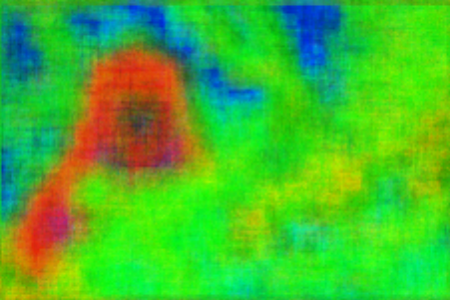
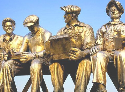
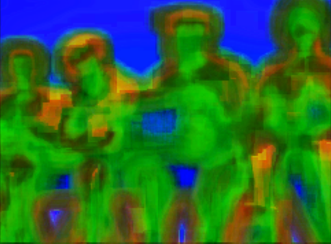
Fuzzy

Organic

Smooth

Shiny

Metallic

Smooth

Figure 2: Per-pixel material trait predictions on unseen test images. Each RGB color channel corresponds to the predicted probability of a single selected material trait. The recognized traits clearly divide the images into regions of similar material appearance. Of particular importance is the fact that we can successfully recognize material properties like “fuzzy” on the left, despite the fact that our training data did not include any animals. The shape of each statue on the right is that of a person, but we see from the recognized material traits that the material is in fact metal.

As preliminary experiment to show that materials do in fact exhibit locally-recognizable visual properties, we use a set of named visual material attributes (visual material traits [27]). By manually annotating images from the FMD with per-pixel masks for 13 material traits, we can then train a set of Randomized Decision Forest [28] classifiers to predict material traits in small local regions. Experimental results show that visual material traits can be recognized very accurately from small ($32\times 32$) image patches, some traits as high as 93.1%, with an average accuracy of 78.4%. Fig. 2 shows sample per-pixel recognition results for a selection of material traits.

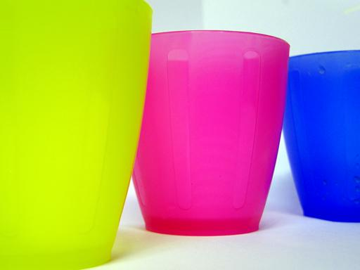
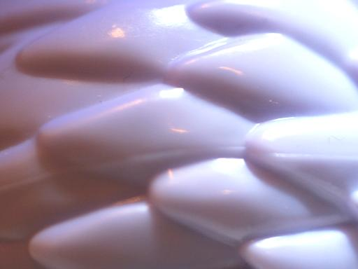
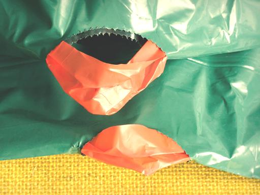
Figure 3: Materials such as the plastic in these images exhibit a wide range of appearances depending on the object and scene. Despite this, we can intuitively recognize visual attributes (smooth and translucent, for example) shared across different instances of the material. In our preliminary work we show that these attributes, which we refer to as visual material traits, are locally-recognizable and can be used to recognize material categories like plastic or metal.

Materials, for example fabric, plastic, or metal, can be challenging to recognize due to the large variation in appearance between instances of the same material. Despite this, looking at the images in Fig. 3, one can see that plastic tends to have visual material attributes that are associated with a distinct appearance, such as “smooth” and “translucent”. Our key observation is that these visual material attributes are recognizable even when the surrounding objects and scenes are not visible. We expect that as a result, we should be able to recognize materials themselves from visual material traits given only small local image patches.

Viewing the full set of material traits as an intermediate representation, we may aggregate them within regions to describe materials. To exploit the material properties found in locally-recognized material traits, we treat the distribution of material traits in a region as an image descriptor and generate a per-image material category prediction. We do so by extracting a number of patches within each material region and using the distributions of traits across these patches as features for a histogram intersection SVM [29]. The average accuracy of this method on 50-50 splits of FMD images is 49.2%. While this is not higher than the accuracy of methods such as [17] that implicitly use context, it is significantly higher than both human and algorithmic performance in the absence of context (38.7-46.9% and 33.8-42.6% respectively respectively [17]). Furthermore, material traits learned from one dataset can be recognized and used to extract material information from an entirely different set, showing that the representation generalizes well.

4 Material Attribute Discovery

Figure 4: Sample material image patches. Asking annotators to merely “describe” the patches is an ambiguous question. Patches may look similar even though the annotator does not have a concrete word to define the similarity. We instead ask only for binary visual similarity decisions.

Material trait recognition relies on a set of fully labeled material trait examples. This assumption hinders scaling the method to larger training datasets. We also do not have a complete, mutually-agreeable vocabulary for describing materials and their visual characteristics; named material traits are merely one attempt at describing material appearance. This makes scaling with multiple annotators difficult. Considering the images in the first column of Fig. 4, for instance, one annotator may call them fuzzy and others may call them fluffy. People may also be inconsistent in annotating material traits. Some may only annotate the patches in the second column as smooth and others may only see them as translucent. Cimpoi et al. [10] alleviate these problems for texture recognition by preparing a pre-defined vocabulary. They may do so by focusing on apparent texture patterns like stripes and dots. Materials underlie these texture patterns (i.e., the stripes or dots on a plastic cup are still plastic) and do not follow such a vocabulary.

Our goal is to discover a set of attributes that exhibit the desirable properties of material traits. We want to achieve this without relying on fully-supervised learning. Known material traits, such as “smooth” or “rough,” represent visual properties shared between similar materials. We expect that attributes that preserve this similarity will satisfy our goal. We propose to define a set of attributes based on the perceived distances between material categories. By working with distances rather than similarities, we avoid any need to assume a particular similarity function. For this, we obtain a measurement of these distances from human annotations.

From a high-level perspective, our attribute discovery consists of three steps:

1. Measure perceptual distances between materials

2. Define an attribute space based on perceptual distances

3. Train classifiers to reproduce this space from image patches

Defining perceptual distance between material categories poses a challenge. If each material had a single typical appearance (e.g., if metal was always shiny and gray), we could simply compute the difference between these typical appearances. This is not the case. Materials may exhibit a wide variety of appearances, even sharing appearances between categories (what we refer to as material appearance variability). An image patch from a leaf, for example, may appear similar to certain fabrics or plastics.

4.1 Measuring Perceptual Distances

Directly measuring distances via human annotation would be ideal, as we have an intuitive understanding of the differences between materials. As Sharan et al. [17] showed, this understanding persists even in the absence of object cues. It is, however, also a difficult task to obtain these distance. Given two query image patches, annotators would have to decide how different the patches look on a consistent quantitative scale. We would instead like to ask simple questions that can be reliably answered.

We propose that instead of asking how different patches look, we reduce the question to a binary one: “Do these patches look different or not?” We assume that this will give us sufficient information to obtain consistent and sensible perceptual information. Our underlying assumption for this claim is that if a pair of image patches look similar, they do so as a result of at least one shared visual material trait.

To transform a set of binary similarity annotations into pairwise distances, we represent each material as a point defined by the average probabilities of similarity to each material category. The pairwise distances between these points define the material perceptual distance matrix. This process treats each material category as a point in a space of typical (but not necessarily realizable) material appearances. The resulting distance between a pair of materials depends on joint similarity with all material categories, including the pair in question, and is thus robust to material appearance variability.

Formally, given a set of $N$ reference images with material category $c_{n}\in\left\{1\ldots K\right\}$, we obtain binary similarity decisions $\mathbf{s}_{n}\in\left\{0,1\right\}^{K}$ for each reference image against a set of sample images from each category. We represent each material category in the space of typical material category appearances as $K$-dimensional vectors $\mathbf{p}_{k}$:

$$\mathbf{p}_{k}=\frac{1}{N_{k}}\sum_{n|c_{n}=k}\mathbf{s}_{n}\text{,}$$ (1)

where $N_{k}=\left|\left\{c_{n}|c_{n}=k\right\}\right|$. Entries $d_{kk^{\prime}}$ in the $K\times K$ pairwise distance matrix $D$ are then defined as:

$$d_{kk^{\prime}}=\left\|\mathbf{p}_{k}-\mathbf{p}_{k^{\prime}}\right\|_{2}\text{.}$$ (2)

We obtain the required set of binary similarity annotations through Amazon Mechanical Turk (AMT). Each task presents annotators with a reference image patch of a given material category (unknown to the annotator) and a row of random image patches, one from each material category. We use patches from images of the 10 material categories from the Flickr Materials Database of Sharan et al. [14]. Annotators are directed to select image patches that look similar to the reference. Examples of suggested similar image patches are given based on known material traits. Each set of patches is shown to 10 annotators, and final results are obtained from a vote where at least 5 annotators must agree that the patches look similar. We collect similarity decisions for 10,000 reference image patches.

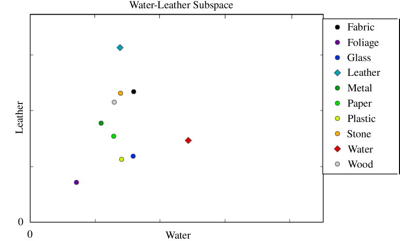
Figure 5: Projection of materials into a 2D similarity subspace allow us evaluate our collected annotations. Coordinates indicate perceived similarity to water and leather respectively. The locations of the two material categories corresponding to the axes are marked. We would expect that, in this case, water would lie furthest along the “water” axis and likewise with leather. We can also see that water occasionally looks like leather. Materials with common visual properties, such as the smoothness of plastic and glass, tend to lie close to each other. Finally, no material appears strongly similar to both leather and water. This is expected as the two materials do generally exhibit different appearances.

The 2D projection in Fig. 5 shows that the similarity values obtained from the AMT annotations agree with our own intuitive understanding of material appearance. The plot shows the locations of material categories projected into one 2D subspace of the 10-dimensional space of material appearance similarity (each dimension corresponding to similarity with that material). We would expect that the two materials corresponding to the axes of their subspace will lie close to their respective axes. In this case, water is most similar with itself, but is also similar to glass. Leather is likewise most similar with itself, but also similar to fabric.

To show that we do in fact obtain a consistent distance matrix, we compute the difference between the distance matrix computed with all annotations versus that from only $n$ of the $N$ total annotations. The difference drops quickly (within the first few hundred samples of 10,000), showing that annotators agree on a single common set of perceptual distances.

4.2 Defining the Material Attribute Space

Discovering attributes given only a desired distance matrix poses a challenge. First, we have no definitions for the attributes since we are trying to discover them from examples of materials. Even if we had such definitions, we have no knowledge of any association between the attributes and the materials. A straightforward approach might be to directly train classifiers to output attribute values that encode the distance matrix. This would be a particularly under-constrained problem given the aforementioned lack of labels or associations.

We instead propose to separate attribute association and classifier learning into two steps. First, we discover attributes in an abstract form by discovering a mapping between categories and attribute probabilities. This mapping places each material category into an attribute space. We ensure that the mapping preserves the pairwise perceptual material distances, and then train classifiers to predict the presence of these attributes on image patches.

As described in Section 4.1, we obtain a distance matrix $\mathbf{D}$ from crowdsourced similarity answers for $K$ material categories $C=\left\{1\ldots K\right\}$. Using $\mathbf{D}$, we find a mapping that indicates which attributes are associated with which categories. The number of attributes we discover is arbitrary, and we refer to it as $M$. The mapping is encoded in the $K\times M$ category-attribute matrix $\mathbf{A}$. We restrict values in $\mathbf{A}$ to lie in the interval $\left[0,1\right]$ so that we may treat them as conditional probabilities.

We impose two constraints on the category attribute mapping. $\mathbf{A}$ should map categories to attributes in a way that preserves the measured distances in $\mathbf{D}$, and the mapping should contain realizable values. If the values in $\mathbf{A}$ are not plausible, we will not be able to recognize the attributes on image patches. For example, one potential attribute mapping would be to assign each attribute to a single category. Attribute recognition would then become material category recognition on single image patches, which is not feasible.

We formulate the attribute discovery process as a minimization problem over category-attribute matrices $\mathbf{A}$:

$$\mathbf{A}^{*}=\arg\min_{\mathbf{A}}d\left(\mathbf{D};\mathbf{A}\right)+w_{A}\kappa_{A}\left(\mathbf{A}\right)$$ (3)

with hyperparameter $w_{A}$. $d$ describes how well the current estimate of $\mathbf{A}$ encodes the pairwise perceptual differences between material categories, and $\kappa_{A}$ is a constraint that makes the discovered attribute associations exhibit a realizable distribution.

The category-attribute matrix that best encodes the desired pairwise distances will minimize the following term defined over rows $\mathbf{a}_{k}$ of the matrix $\mathbf{A}$:

$$d\left(\mathbf{D};\mathbf{A}\right)=\sum_{k,k^{\prime}\in C}\left(\left\|\mathbf{a}_{k}-\mathbf{a}_{k^{\prime}}\right\|_{2}-\mathbf{D}_{kk\prime}\right)^{2}\text{.}$$ (4)

To discover realizable attributes, we encode our own prior knowledge that recognizable attributes exhibit a particular distribution and sparsity pattern. We observe that semantic attributes, specifically visual material traits, have a Beta-distributed association with material categories. Generally, a material category will either strongly exhibit a trait or it will not exhibit it at all. Intermediate cases occur when a material category exhibits a particularly wide variation in appearance. Fabric, for example, sometimes has a clear “woven” pattern but, in the case of silk or other smooth fabrics, does not. We would like the values in $\mathbf{A}$ to be Beta-distributed to match the distribution of known material trait associations.

The canonical method for matching two distributions is to minimize a divergence measure between them. To incorporate this into a minimization formulation, we need a differentiable measurement for the unknown empirical distribution of values in $\mathbf{A}$. We choose the KL-divergence and Gaussian kernel density estimator. The Gaussian kernel density estimate at point $p$ is:

$$q\left(p;\mathbf{A}\right)=\frac{1}{KM}\sum_{k,m}\left(2\pi h^{2}\right)^{-\frac{1}{2}}\exp\left\{-\frac{\left(a_{km}-p\right)^{2}}{2h^{2}}\right\}$$ (5)

The KL-divergence between the distribution of the values in the category-attribute matrix $\mathbf{A}$ and the target Beta distribution $\beta\left(p;a,b\right)$ with $a=b=0.5$ can then be written as:

$$\kappa_{A}\left(\mathbf{A}\right)=\sum_{p\in P}\beta\left(p;a,b\right)\ln\left(\frac{\beta\left(p;a,b\right)}{q\left(p;\mathbf{A}\right)}\right)\text{.}$$ (6)

4.3 Training a Material Attribute Classifier

We now must derive classifiers that recognize the attributes defined by the category-attribute mapping. As attributes are not defined semantically, we cannot ask for further annotation to label training patches with attributes. Instead, we propose a model and a set of constraints that will enable us to predict our discovered attributes on material image patches.

We do not know a priori any particular semantics or structure associated with the attributes, thus we model our attributes using a general two-layer non-linear model [30]. We constrain the predictions such that they reproduce the desired values in the attribute matrix (in expectation) while also separating material categories when possible.

Formally, given a training set of $N$ image patches represented by $D$-dimensional raw feature vectors $\mathbf{x}_{n}$ with corresponding material categories $c_{n}\in C$, we train a model $f$ with parameters $\mathbf{\Theta}$ that maps an image patch to $M$ attribute probabilities: $f\left(\mathbf{x}_{n};\mathbf{\Theta}\right):\mathbb{R}^{D}\rightarrow\left[0,1\right]^{M}$. Given an intermediate layer with dimensionality $H$ and parameters $\mathbf{W}_{1}\in\mathbb{R}^{H\times D}$, $\mathbf{W}_{2}\in\mathbb{R}^{M\times H}$, $\mathbf{b}_{1}\in\mathbb{R}^{H}$, $\mathbf{b}_{2}\in\mathbb{R}^{M}$ the prediction for an instance $\mathbf{x}_{n}$ is defined as:

$$f\left(\mathbf{x}_{n};\mathbf{\Theta}\right) = h\left(\mathbf{W}_{2}h\left(\mathbf{W}_{1}\mathbf{x}_{n}+\mathbf{b}_{1}\right)+\mathbf{b}_{2}\right)$$

$$h\left(x\right) = \min\left(\max\left(x,0\right),1\right)\text{.}$$ (7)

As additional regularization, used only during training, we mask out a random fraction of the weights used in the model to discourage overfitting (akin to dropout [31]).

We formulate the full classifier training process as a minimization problem:

$$\mathbf{\Theta}^{\star}=\arg\min_{\mathbf{\Theta}}r\left(\mathbf{X};\mathbf{A},\mathbf{\Theta}\right)+w_{1}\kappa\left(\mathbf{X};\mathbf{\Theta}\right)-$$

$$w_{2}\pi\left(\mathbf{X};\mathbf{A},\mathbf{\Theta}\right)\text{,}$$ (8)

with hyperparameters $w_{1}$ and $w_{2}$. $r$ (Equation 9) is a data term indicating the difference between predicted and expected attribute probabilities. $\kappa$ and $\pi$ (Equations 10 and 11) are, respectively, constraints on the the distribution of attribute predictions and on the pairwise separation of material categories.

The category-attribute matrix encodes the probabilities that each category will exhibit each attribute. We represent this in our classifier training by matching the mean predicted probability for each attribute to the given entry in the category-attribute matrix:

$$r\left(\mathbf{X};\mathbf{A},\mathbf{\Theta}\right)=\sum_{k\in C}\left\|\mathbf{a}_{k}-\frac{1}{N_{k}}\sum_{i|c_{i}=k}f\left(\mathbf{x}_{i};\mathbf{\Theta}\right)\right\|_{2}^{2}\text{.}$$ (9)

Equation 9 directly encodes the desired behavior of the classifier, but it alone is under-constrained. Each prediction for each instance may take on any value so long as their mean matches the target value.

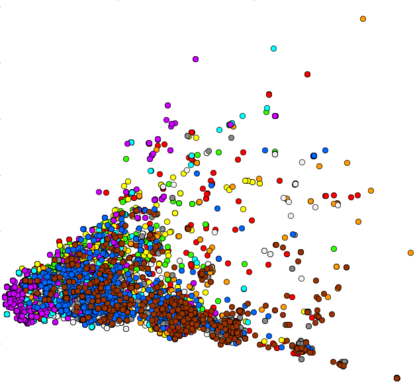
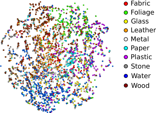
(a) Raw Features (b) Discovered Attribute Predictions

Figure 6: t-SNE [32] embedding of materials from the raw feature space (a) and from our discovered attributes (b). We embed a set of material image patches into 2D space via t-SNE using raw features and predicted attribute probabilities as the input space for the embeddings. Though t-SNE has been shown to perform well in high-dimensional input spaces, it fails to separate material categories from the raw feature space. Material categories are, however, clearly more separable with our attribute space.

We have observed that, similar to category-attribute associations, predicted probabilities for known material traits are also Beta-distributed. Local image regions exhibiting a trait will have uniformly high probability for that trait, only decreasing around the trait region edges. We constrain the predicted probabilities such that they are Beta-distributed. Using the formulation discussed in Section 4.2, we again minimize a KL-divergence of a kernel density estimate:

$$\kappa\left(\mathbf{X};\mathbf{\Theta}\right)=\sum_{p\in P}\beta\left(p;a,b\right)\ln\left(\frac{\beta\left(p;a,b\right)}{q\left(p;f\left(\mathbf{X};\mathbf{\Theta}\right)\right)}\right)\text{,}$$ (10)

where $f\left(\mathbf{X};\mathbf{\Theta}\right)$ represents the $N\times M$ matrix of attribute probability predictions for the training dataset, and $q,a,b$ are defined as in Equation 6.

One of the goals for our attribute representation is to discover attributes that allow for material classification. If this were our only goal, we could simply maximize the distance between the predicted attributes for all pairs of different material categories. This would conflict with our goal of preserving human perception, as material categories do not always exhibit different appearances. We instead modify this separation by weighting each component of the distance based on the values in the category-attribute matrix:

$$\pi\left(\mathbf{X};\mathbf{A},\mathbf{\Theta}\right)=\sum_{i,j\in N|c_{i}\neq c_{j}}\mathbf{p}_{ij}^{\mathrm{T}}\mathbf{p}_{ij}$$ (11)

$$\mathbf{p}_{ij}=\left(2\left|\mathbf{a}_{c_{i}}-\mathbf{a}_{c_{j}}\right|-1\right)\left(f\left(\mathbf{x}_{i};\mathbf{\Theta}\right)-f\left(\mathbf{x}_{j};\mathbf{\Theta}\right)\right)\text{.}$$

This separates the material categories in attribute space only when the attributes dictate that there is a perceptual difference.

4.4 Analysis of Discovered Attributes

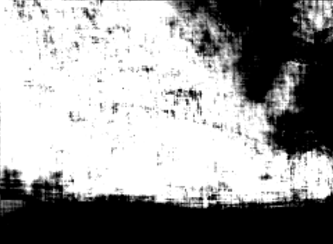
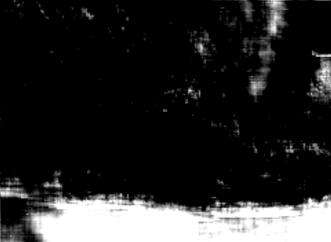
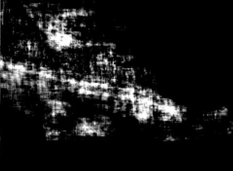
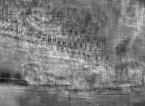
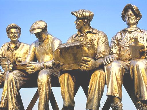
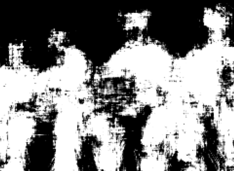
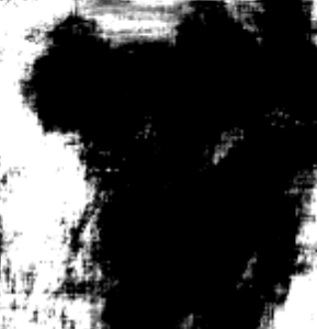
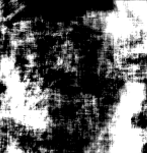
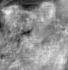
Input   Attribute 1 Attribute 2 Attribute 3   Random

Figure 7: Per-pixel discovered attribute probabilities for four attributes (one per column). These images show that the discovered attributes exhibit patterns similar to those of known material traits. The first attribute, for example, appears consistently within the woven hat and the koala; the second attribute tends to indicate smooth regions. The third attribute shows we are discovering attributes that can appear both sparsely and densely in an image, depending on the context. These are all properties shared with visual material traits. Attributes from a random $\mathbf{A}$ do not exhibit any of these properties.

To analyze the properties of attributes discovered by our framework, we follow the procedures outlined above to collect annotations and discover a set of attributes. Since both learning steps involve minimization of a non-linear, non-convex function, we rely on existing optimization tools to find suitable estimates. As a raw feature set, we use the local features we developed for material trait recognition (Section 3).

If our attributes described a space that successfully separates material categories, we would expect categories to form clusters in the attribute space. To verify this, we compute a 2D embedding of a set of labeled image patches. For the embedding, we use the t-SNE method of van der Maaten and Hinton [32]. t-SNE attempts to generate an embedding that matches the distributions of neighboring points in the high- and low-dimensional spaces. In Fig. 6, we represent image patches by their raw feature vectors (a) and predicted attribute probability vectors (b), and compare the 2D embeddings resulting from each. Material categories are separated much more clearly in our attribute space than in the raw feature space.

Part of the usefulness of visual material traits, as we have shown above, is derived from the fact that they each represent a particular intuitive visual material property. This is evident in the spatial sparsity pattern of the traits, specifically the fact that they appear in regions and not randomly within an image. Traits such as “shiny” are highly localized, while others such as “woven” or “smooth” exist as coherent regions within a particular material instance. Fig. 7 shows examples of per-pixel attribute probabilities predicted from our discovered attribute classifiers. The attributes exhibit both sparse and dense spatial patterns that are consistent within local regions. Dense attributes generally correspond with smooth image regions. Sparse attributes often indicate localized surface features such as specific texture patterns.

Randomized features have been shown to provide a viable representation for classification tasks [33]. Despite this, we expect that such features would not be likely to encode the same perceptual properties as our attributes. We can demonstrate this by replacing our perceptually-derived attribute matrix $\mathbf{A}$ with randomized matrix of the same shape. The last column in Fig. 7 shows typical results for such a matrix. Unlike attributes based on human perception, these random attributes do not exhibit any of the desired perceptual properties like spatial consistency.

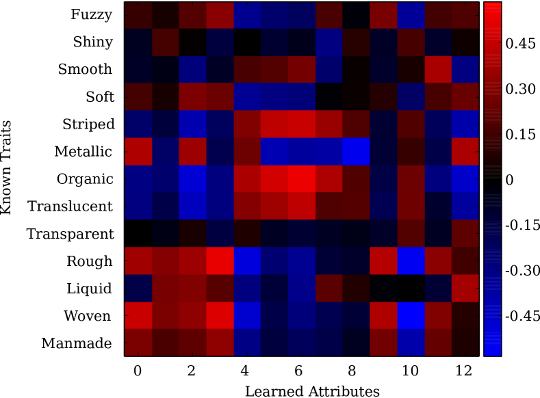
Figure 8: Correlation between discovered attribute predictions and material traits. Groups of attributes can collectively indicate the presence of a material trait. Metallic, for example, correlates positively with attribute 0 and negatively with attribute 8.

We aimed to discover attributes similar to the visual material traits that underlie human perception. We thus expect that the discovered attributes exhibit a correlation with known traits. Fig. 8 shows the correlation between 13 discovered attributes and 13 known material traits using attributes predicted on labeled material trait image patches. Collectively, we can indeed describe material traits using the discovered attributes. Visually similar traits, such as rough and woven, show similar correlations with the attributes. Discovered attributes are also consistent with the semantic properties of material traits. Rough and smooth are mutually exclusive traits, and we see that discovered attributes that positively correlate with smooth do not generally correlate with rough.

We quantitatively evaluate the discovered attributes using logic regression [34]. Given a set of image patches with known traits, we predict our discovered attributes as binary values for use as input variables in a logic regression model for material traits. Logic regression from 30 attributes alone (no other features) achieves comparable accuracy to our trait-based method and its complex feature set. These results show that the discovered attributes do collectively encode intuitive visual material properties. Further details and examples of logic regression to predict material traits can be found in Sec. 7.1.

4.5 From Discovered Attributes to Materials

Seeing that discovered attributes encode visual material properties, we would expect them to also serve as an intermediate representation for material category recognition. To test this, we follow our local material recognition procedure (Section 3), substituting our discovered attributes in place of labeled material traits. We compute the histograms of these predicted probabilities across the material region and use them as input for a histogram kernel SVM. As we focus on local attributes, these previous local results (and those of Sharan et al. [17] on scrambled images) serve as the correct baseline.

To compare with our previous results using material traits, we compute average material recognition accuracy on the Flickr Materials Database (FMD). All results are computed using $M=30$ discovered attributes and 5-fold cross-validation unless otherwise specified.

Our attributes achieve an average accuracy of 48.9% ($\sigma=1.2\%$) on FMD images using only local information. This is comparable to our results and those of Sharan et al. [17] (using only local information) even though we are discovering attributes using only weak supervision.

Looking at individual class recognition rates, metal is the most challenging category to identify while foliage is the most accurately recognized. This follows from the results of our measurements of human perception, as annotators consistently found that foliage image patches looked different from all other material categories. Metal is particularly difficult to recognize locally as its appearance depends strongly on the appearance of the surround environment (due to specular reflection).

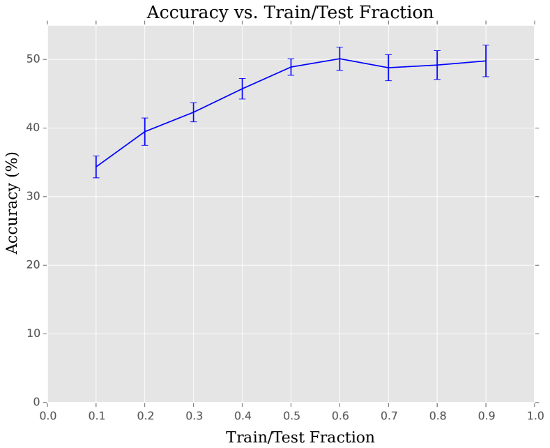
Figure 9: Accuracy vs. training set size. The line is the average of 3 random splits. Error bars indicate the minimum and maximum of the splits. Accuracy does not continue to increase as we use larger training datasets. This shows that we have successfully extracted as much local information as possible from human perception.

Fig. 9 shows that accuracy reaches a plateau as the training dataset size increases. We also compute accuracy for varying values of $M$ and find that past $M=30$, there is little (<0.1%) gain in accuracy from additional attributes. These results indicate that we are in fact extracting as much perceptual material information as we can from the available data.

5 Perceptual Material Attributes in Convolutional Neural Networks

We have shown that we may use visual material traits to enable local material recognition, and we may further scale this attribute-based recognition process by automatically discovering perceptual material attributes. Our previous methods consider attributes separately from category recognition. The attributes are used solely as an intermediate representation for material categories. Similarly for conventional object and scene recognition, attributes like “sunset” or “natural,” have also been extracted for use as independent features. Shankar et al. [23] generate pseudo-labels to improve the attribute prediction accuracy of a Convolutional Neural Network, and Zhou et al. [25] discover concepts from weakly-supervised image data. In both cases, the attributes are considered on their own, not within the context of higher-level categories. In object and scene recognition, however, recent work shows that semantic attributes seem to arise in networks that are trained end-to-end for category recognition [35].

We would like to take advantage of the benefits of end-to-end learning to incorporate automatically-discovered attributes with material recognition in one seamless process. Material attribute recognition, however, is not easily scalable. In the past we relied on semantic attributes, such as “shiny” or “fuzzy”, that needed careful annotation by a consistent annotator as their appearance may not be readily agreed upon. We addressed the difficulty in annotation scaling by automatically discovering perceptual material attributes from weak supervision. The training process for this method does not, however, scale well to large datasets. To address this, we propose a novel CNN architecture that recognizes materials from small local image patches while producing perceptual material attributes as an auxiliary output. We also introduce a novel material database with material categories drawn from a materials-science-based category hierarchy.

5.1 Finding Material Attributes in a Material Recognition CNN

Hiramatsu et al. [5] have shown that perceptual attributes form an integral component of the human material recognition process. They found that during the process of material recognition, we form a perceptual representation of materials analogous to the intermediate representation provided by named material traits or automatically-discovered material attributes. The key difference is that the perceptual representation in human material recognition forms as an integral part of the recognition process.

Our goal is to discover unnamed material attributes while performing material recognition in one end-to-end scalable process. Based on correlations between Convolutional Neural Network (CNN) feature maps and human visual system neural output discovered by Yamins et al. [26], a CNN architecture appears to be a very suitable framework in which to discover attributes analogous to those in human material perception. Their work focuses on object recognition, however, and does not extract any attributes. In this case, our automatically-discovered unnamed material attributes are particularly relevant. We derive a novel framework to discover perceptual attributes similar to the ones we describe in Section 4 inside a material recognition CNN framework.

A simple experiment to verify the feasibility of perceptual attribute discovery in a CNN trained to recognize materials would be to add a layer at the top of the network, immediately before the final material category probability softmax layer, and constrain this layer to output the same attributes we previously discovered in a separate process. If we could predict attributes from this layer without affecting the material recognition accuracy, this would suggest that we could indeed combine attribute discovery and material recognition. We implemented this approach and found that while the material accuracy was unaffected, the attribute predictions were less accurate than if the CNN was trained solely to predict the attributes and not materials as well (mean average error of 0.2 vs 0.08).

The key issue with the straightforward approach is that it is not an entirely faithful model to the process described in [5]. They note that the human neural representation of material categories transitions from visual (raw image features) to perceptual (visual properties like “shiny”) in an hierarchical fashion. This implies, in agreement with findings of Escorcia et al. [24], that attributes require information from multiple levels of the material recognition network. We show that this is indeed the case by successfully discovering the attributes using input from multiple layers of the material recognition network.

5.2 Material Attribute-Category CNN

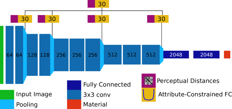
Figure 10: Material Attribute-Category CNN (MAC-CNN) Architecture: We introduce auxiliary fully-connected attribute layers to each spatial pooling layer, and combine the per-layer predictions into a final attribute output via an additional set of weights. The loss functions attached to the attribute layers encourage the extraction of attributes that match the human material representation encoded in perceptual distances. The first set of attribute layers acts as a set of weak learners to extract attributes wherever they are present. The final layer combines them to form a single prediction.

We need a means of extracting attribute information at multiple levels of the network. Simply combining all feature maps from all network layers and using them to predict attributes would be computationally-impractical. Rather than directly using all features at once, we augment an initial CNN designed for material classification with a set of auxiliary fully-connected layers attached to the spatial pooling layers. This allows the attribute layers to use information from multiple levels of the network without needing direct access to every feature map. We treat the additional layers as a set of weak learners, each auxiliary layer discovering the attributes available at the corresponding level of the network. This is similar to the deep supervision of Lee et al. [36]. Their auxiliary loss functions, however, simply propagate the same classification targets (via SVM-like loss functions) to the lower layers. Rather than propagating gradients, our attribute layers discover perceptual material attributes.

For the auxiliary layer loss functions, we introduce a modified form of the perceptual attribute loss function (Equation 8) to the outputs of each auxiliary fully-connected layer. Specifically, assuming the output of a given pooling layer $i$ in the network for image $j$ is $\mathbf{h}_{ij}$, and given categories $C,\,\left|C\right|=K$ and a set of sample points $P\in\left(0,1\right)$ for density estimation, we add the following auxiliary loss functions:

$$u_{i}=\frac{1}{K}\sum_{k\in C}\left\|\mathbf{a}_{k}-\frac{1}{N_{k}}\sum_{j|c_{j}=k}f\left(\mathbf{W}_{i}^{\mathrm{T}}\mathbf{h}_{ij}+\mathbf{b}_{i}\right)\right\|_{1}$$ (12)

$$d_{i}=\sum_{p\in P}\beta\left(p;a,b\right)\ln\left(\frac{\beta\left(p;a,b\right)}{q\left(p;f\left(\mathbf{W}_{i}^{\mathrm{T}}\mathbf{h}_{ij}+\mathbf{b}_{i}\right)\right)}\right)\text{,}$$ (13)

where $f\left(x\right)=\min\left(\max\left(x,0\right),1\right)$ clamps the outputs within $\left(0,1\right)$ to conform to attribute probabilities, and weights $\mathbf{W}_{i},\mathbf{b}_{i}$ represent the auxiliary fully-connected layers we add to the network. $\mathbf{a}_{k}$ represents a row in the category-attribute mapping matrix derived as in Section 4.2. Equation 12 causes the attribute layer to discover attributes which match the perceptual distances measured from human annotations. As certain attributes are expected to appear at different levels of the network, some layers will be unable to extract them. This implies that their error should be sparse, either predicting an attribute well or not at all. For this reason we use an L1 error norm. Equation 13, applied only to the final attribute layer, encourages the distribution of the attributes to match those of known semantic material traits. It takes the form of a KL-divergence between a Beta distribution (empirically observed to match the distribution of semantic attribute probabilities), and a Kernel Density Estimate $q\left(\cdot\right)$ of the extracted attribute probability density sampled at points $p\in P$.

The reference network we modify is based on the high-performing VGG-16 network of Simonyan and Zisserman [21]. We use their trained convolutional weights as initialization where applicable, and add new fully-connected layers for material classification. Fig. 10 shows our architecture for material attribute discovery and category recognition. We refer to this network as the Material Attribute-Category CNN (MAC-CNN).

6 Local Material Database

In order to train the category recognition portion of the MAC-CNN, we need a suitable dataset, and we find existing material databases lacking in a few key areas. Previous material recognition datasets [17, 19, 20] have relied on ad-hoc choices regarding the selection and granularity of material categories. When patches are involved, as in [20], the patches can be as large as 24% of the image size surrounding a single pixel identified as corresponding to a material. These patches are large enough to include entire objects. These issues make it difficult to separate challenges inherent to material recognition from those related to general recognition tasks. Materials, as with their visual attributes, are inherently local properties. While knowledge of what object the material composes may help recognize the material, the material is not the object. We also find that image diversity is still lacking in these modern datasets. For these reasons, we introduce a new local material recognition dataset to support the experiments in this paper.

6.1 Material Category Hierarchy

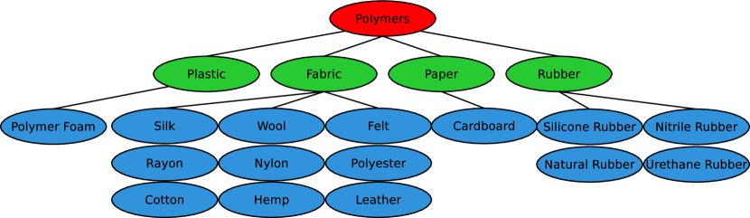
Figure 11: One tree in our material category hierarchy. Categories at the top level separate materials with notable differences in physical properties. Mid-level categories are visually distinct. The lowest level of categories are fine-grained and may require both physical and visual properties and expert knowledge to distinguish them.

Material categories in existing datasets have not been carefully selected. Examples of this appear in the recent work of Bell et al. [20], where proposed material categories include “mirror” and “carpet” (among others). These are in fact objects, and their annotations reflect this. Their categories also confuse materials and their visual properties, for example, separating “stone” from “polished stone”. To address the issue of material category definition, we propose a set of material categories derived from a materials science taxonomy. Additionally, we create a hierarchy based on the generality of each material family. Fig. 11 shows an example of one tree of the hierarchy.

Our hierarchy consists of a set of three-level material trees. The highest level corresponds to major structural differences between materials in the category. Metals are conductive, polymers are composed of long chain molecules, ceramics have a crystalline structure, and composites are fusions of materials either bonded together or in a matrix. We define the mid-level (also referred to as entry-level [37]) categories as groups that separate materials based primarily on their visual properties. Rubber and paper are flexible, for example, but paper is generally matte and rubber exhibits little color variation. The lowest level, fine-grained categories, can often only be distinguished via a combination of physical and visual properties. Silver and steel, for example, may be challenging to distinguish based solely on visual information.

Such a hierarchy is sufficient to cover most natural and manmade materials. In creating our hierarchy, however, we found that certain categories that are in fact materials did not fit within the strict definitions described above. For the sake of completeness, we make the conscious decision to add these mid-level categories to our data collection process. These categories are: food, water, and non-water liquids. While food is both a material and an object, we rely on our annotation process (Sec. 6.2) to ensure we obtain examples of the former and not the latter.

6.2 Data Collection and Annotation

The mid-level set of categories forms the basis for a crowdsourced annotation pipeline to obtain material regions from which we may extract local material patches. We employ a multi-stage process to efficiently extract both material presence and segmentation information for a set of images.

The first stage asks annotators to identify materials present in the image. Given a set of images with materials identified in each image, the second stage presents annotators with a user interface that allows them to draw multiple regions in an image. Each annotator is given a single image-material pair and asked to mark regions where that material is present. While not required, our interface allows users to create and modify multiple disjoint regions in a single image. Images undergo a final validation step to ensure no poorly drawn or incorrect regions are included.

Each image in the first stage is shown to multiple annotators and a consensus is taken to filter out unclear or incorrect identifications. While sentinels and validation were not used to collect segmentations in other datasets, ours is intended for local material recognition. This implies that identified regions should contain only the material of interest. During collection, annotators are given instructions to keep regions within object boundaries, and we validate the final image regions to insure this.

Image diversity is an issue present to varying degrees in current material image datasets. The Flickr Materials Database (FMD) [14] contains images from Flickr which, due to the nature of the website, are generally more artistic in nature. The OpenSurfaces and Materials in Context datasets [19, 20] attempt to address this, but still draw from a limited variety of sources. We source our images from multiple existing image datasets spanning the space of indoor, outdoor, professional, and amateur photographs. We use images from the PASCAL VOC database [38], the Microsoft COCO database [39], the FMD [14], and the imagenet database [40].

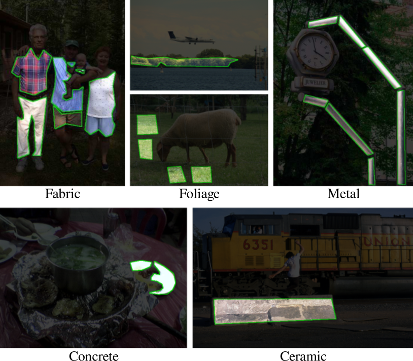
Figure 12: Example annotation results. Annotators did not hesitate to take advantage of the ability to draw multiple regions, and most understood the guidelines concerning regions crossing object boundaries. As a result, we have a rich database of segmented local material regions.

Examples in Fig. 12 show that our annotation pipeline successfully provides properly-segmented material regions within many images. Many images also contain multiple regions. While the level of detail for provided regions varies from simple polygons to detailed material boundaries, the regions all contain single materials.

Our database currently contains 5845 images with carefully-segmented material regions. For comparison, the MINC [20] database does not provide any segmented material regions for training, and only 1798 images for testing.

7 Visual Material Attributes Discovered in the MAC-CNN

To verify that the visual material attributes we seek are indeed present in and can be extracted with our MAC-CNN, we augment our dataset with annotations to compute the necessary perceptual distances described in Section 4.1. Using our dataset and these distances, we derive a category-attribute matrix $\mathbf{A}$ and train an implementation of the MAC-CNN described in Section 5.2.

We train the network on ~200,000 $48\times 48$ image patches extracted from segmented material regions. Optimization is performed using mini-batch stochastic gradient descent with momentum. The learning rate is decreased by a factor of 10 whenever the validation error increases, until the learning rate falls below $1\times 10^{-8}$.

7.1 Properties of MAC-CNN Visual Material Attributes

We examine the properties of our visual material attributes by visualizing how they separate materials, computing per-pixel attribute maps to verify that the attributes are being recognized consistently, and linking the non-semantic attributes with known semantic material traits (“fuzzy”, “smooth”, etc…) to visualize semantic content. Figs. 13, 14, and 15 are generated using a test set of held-out images.

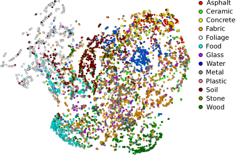
Figure 13: Attribute Space Embedding via t-SNE [32]: Many categories, such as water, food, foliage, soil, and wood, are extremely well-separated in the attribute space. We find that this separation corresponds with per-category accuracy: well-separated categories are recognized more accurately. While other categories do overlap to some extent, they still form separate regions in the space.

A 2D embedding of material image patches shows that the attributes (Fig. 13) separate material categories. A number of materials are almost completely distinct in the attribute space, while a few form overlapping but still distinguishable regions. Foliage, food, and water form particularly clear clusters. The quality of the clusters correlates with category recognition accuracy, with accurately-recognized categories forming well-separated clusters.

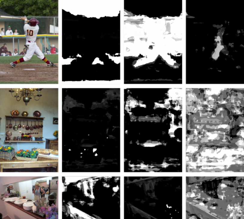
Figure 14: The attributes from the MAC-CNN (visualized to the right of an input image above) exhibit the same properties as our the attributes we previously discovered independent of material recognition. The attributes form clearly delineated regions, similar to semantic attributes, and their distributions match as well.

Visualizations of per-pixel attribute probabilities in Fig. 14 show that the attributes are spatially consistent. While overfitting is difficult to measure for weakly-supervised attributes, we use spatial consistency as a proxy. Spatial consistency is an indicator that the attributes are not overly-sensitive to minute changes in local appearance, something that would appear if overfitting were present. The attributes exhibit correlation with the materials that induced them: attributes with a strong presence in a material region in one image often appear similarly in others. The visualizations also clearly show that the attributes are representing more than trivial properties such as “flat color” or “bumpy texture”.

  Manmade     Organic     Rough

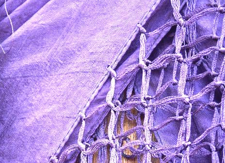
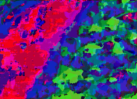
  Smooth     Striped     Soft

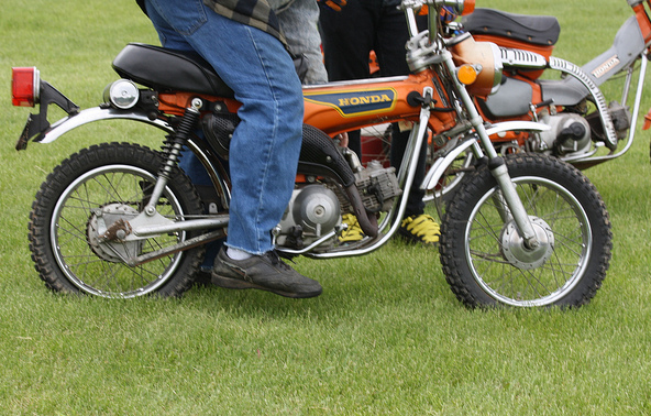
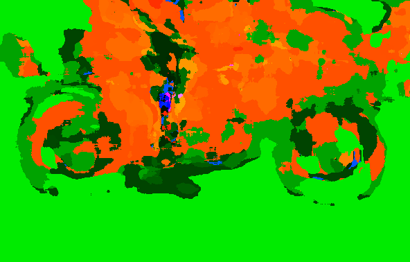
  Metallic     Organic     Smooth

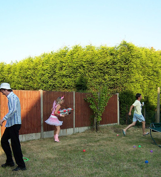
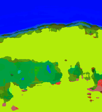
  Fuzzy     Organic     Smooth

Figure 15: By performing logic regression from our MAC-CNN extracted attributes to semantic material traits, we are able to extract semantic information from our non-semantic attributes. We can apply logic regression to material attribute predictions on patches in a sliding window to obtain per-pixel semantic material trait information. The per-pixel trait predictions show crisp regions that correspond well with their associated semantic traits. Traits are independent, and thus the maps contain mixed colors. Fuzzy and organic in the lower right image, for example, creates a yellow tint.

Logic regression [34] is a method for building trees that convert a set of boolean variables into a probability value via logical operations (AND, OR, NOT). It is well-suited for collections of binary attributes such as ours. Results of performing logic regression (Fig. 15) from extracted attribute predictions to known semantic material traits (such as fuzzy, shiny, smooth etc…) show that our MAC-CNN attributes encode material traits with the roughly same average accuracy (77%) as the our previous attributes. We may also predict per-pixel trait probabilities in a sliding window fashion, showing that the attributes are encoding both perceptual and semantic material properties.

7.2 Local Material Recognition

Our results in Section 7 show that we can successfully discover unnamed visual material attributes in the combined material-attribute network. If these discovered attributes were not complete, or if they were not faithfully representing material properties, we would expect material recognition accuracy to improve by removing the attribute discovery constraints. While the attribute layers are auxiliary, they are connected to spatial pooling layers at every level and thus the attribute constraints affect the entire network. We in fact find that the average material category accuracy does not change when the attribute layers are removed.

The average accuracy is 60.2% across all categories. Foliage is the most accurately recognized, consistent with past material recognition results in which foliage is the most visually-distinct category. Paper is the least well-recognized category. Unlike the artistic closeup images of the FMD, many of the images in our database come from ordinary images of scenes. Paper, in these situations, shares its appearance with a number of other materials such as fabric.

It is important to note that we are recognizing materials directly from single small image patches, with none of the region-based aggregation or large patches used before and by other methods [20]. This is a much more challenging task as the available information is restricted. These restrictions are necessary, however, as using large image patches (such as in the MINC database) would cause the attributes we discover to implicitly depend on the objects present in the patches and not simply the materials.

In this paper, our goal is not to introduce a novel material recognition method but rather to investigate the recognition of material properties from images. As such, the correct baseline for comparison is between our previously discovered attributes and those we discover in the MAC-CNN, not material recognition accuracy. Material recognition accuracy is used simply to demonstrate that the discovery of visual material attributes is compatible with material recognition in a single end-to-end trainable network. As we have shown in our parallel work [18], accurate material recognition requires the proper integration of local and global context. Integrating our attribute discovery method with a state-of-the-art material recognition framework that fuses local and global context is one promising avenue for future work.

Soil

Foliage

Fabric

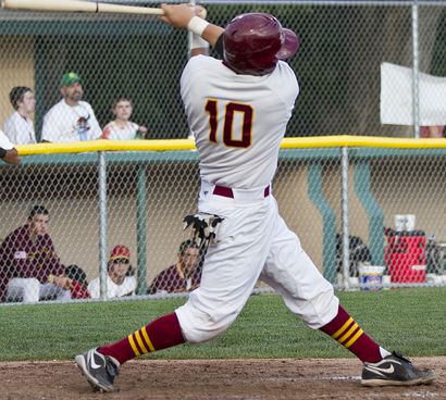
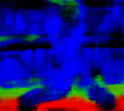
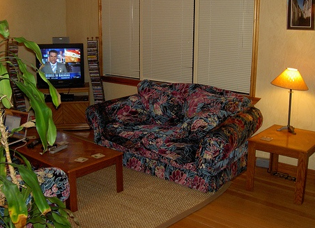
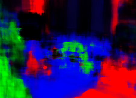
Wood

Foliage

Fabric

Figure 16: Applying the MAC-CNN in a sliding-window fashion leads to a set of material category probability maps. These material maps show that we may obtain coherent regions using only small local patches as input. The foliage predictions in the bottom right image are reasonable, as the local appearance is indeed a flower. In the upper right image, the local appearance of the fence resembles lace (a fabric).

While a full dense per-pixel material segmentation framework is outside the scope of this work, we are able to use the MAC-CNN to produce per-pixel material probability predictions in a sliding window fashion. Results in Fig. 16 show that we may still generate reasonable material probability maps even from purely local information.

7.3 Novel Material Category Recognition

One prominent application of attributes is in novel category recognition tasks. Examples of these tasks include one-shot [41] or zero-shot learning [7]. Zero-shot learning allows recognition of a novel category from a human-supplied list of applicable semantic attributes. Since our attributes are non-semantic, zero-shot learning is not applicable here. We may, however, investigate the generalization of our attributes through a form of one-shot learning in which we use image patches extracted from a small number of images to learn a novel category.

To evaluate the application of visual material attributes for novel category recognition, we train a set of attribute/material networks on modified datasets each containing a single held-out category. No examples of the held-out category are present during training. The corresponding row of the category-attribute matrix is also removed. The same number of attributes are defined based on the remaining categories.

For the novel category training, we use a balanced dataset consisting of unseen examples of training categories and a matching number of images from the held-out category. We also separate a number of images of the held-out category as final testing samples. We train a simple binary classifier (a linear SVM) to distinguish between the training categories and the held-out category based on either their attribute probabilities, material probabilities, or both, computed on patches extracted from each input image. We measure the effectiveness of novel category recognition by the fraction of final held-out category samples properly identified as belonging to that category.

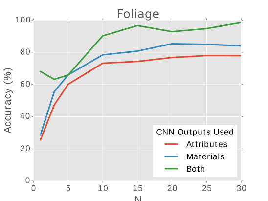
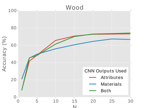
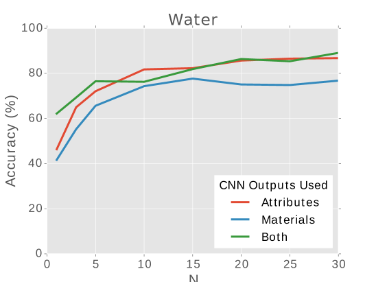
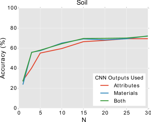
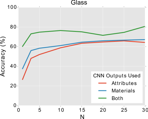
Figure 17: Graphs of novel category recognition accuracy vs. training set size for various held-out categories. The rapid plateau shows that we need only a small number of examples to define a previously-unseen category. The accuracy difference between feature sets shows that the attributes are contributing novel information.

Fig. 17 shows plots of novel category recognition effectiveness as the number of training examples for the held-out category varies. We can see that the accuracy plateaus quickly, indicating that the attributes provide a compact and accurate representation for novel material categories. The number of images we are required to extract patches from to obtain reasonable accuracy is generally quite small (on the order of 10) compared to full material category recognition frameworks which require hundreds of examples. Furthermore, we include accuracy for the same predictions based on only material probabilities instead of attribute probabilities, as well as using a concatenation of both. This clearly shows that the extracted attributes can expose novel information in the MAC-CNN that would not ordinarily be available.

8 Conclusion

Material properties provide valuable cues to guide our everyday interactions with the materials that exhibit them. We aimed to recognize such properties from images, in the form of visual material attributes, so that we might make this information available for general scene understanding. Our goal was not only to recognize these properties, but to do so in a scalable fashion that allows our method to handle modern large-scale material datasets.

By defining and recognizing a novel set of visual material attributes – material traits – we showed that material properties are locally-recognizable and can be aggregated to classify materials in image regions. To scale the annotation process, we introduced a novel method that probes our own perception of material appearance, using only weak supervision in the form of yes/no similarity annotations, to discover unnamed visual material attributes that serve the same function as fully-supervised material traits. Our proposed MAC-CNN allows us to apply our attribute discovery framework to modern large-scale image databases in a seamless end-to-end fashion. Furthermore, the design of the MAC-CNN exposes interesting parallels between human and computer vision.

Gabriel Schwartz is a Ph.D. student at Drexel University in the Department of Computer Science. He received his B.S. and M.S in Computer Science from Drexel University in 2011. His research interests focus on computer vision and machine learning.

Ko Nishino is a professor in the Department of Computing in the College of Computing and Informatics at Drexel University. He is also an adjunct associate professor in the Computer and Information Science Department of the University of Pennsylvania and a visiting associate professor of Osaka University. He received a B.E. and an M.E. in Information and Communication Engineering in 1997 and 1999, respectively, and a PhD in Computer Science in 2002, all from The University of Tokyo. Before joining Drexel University in 2005, he was a Postdoctoral Research Scientist in the Computer Science Department at Columbia University. His primary research interests lie in computer vision and include appearance modeling and synthesis, geometry processing, and video analysis. His work on modeling eye reflections received considerable media attention including articles in New York Times, Newsweek, and NewScientist. He received the NSF CAREER award in 2008.

References

- [1] A. Farhadi, I. Endres, D. Hoiem, and D. Forsyth, “Describing Objects by their Attributes,” in CVPR, 2009, pp. 1778–1785.
- [2] V. Ferrari and A. Zisserman, “Learning Visual Attributes,” in NIPS, 2007, pp. 433–440.
- [3] N. Kumar, P. Belhumeur, and S. Nayar, “FaceTracer : A Search Engine for Large Collections of Images with Faces,” in ECCV, 2008, pp. 340–353.
- [4] G. Patterson and J. Hays, “SUN Attribute Database: Discovering, Annotating, and Recognizing Scene Attributes,” in CVPR, 2012.
- [5] C. Hiramatsu, N. Goda, and H. Komatsu, “Transformation from Image-Based to Perceptual Representation of Materials along the Human Ventral Visual Pathway,” NeuroImage, no. 57, pp. 482–494, 2011.
- [6] N. Goda, A. Tachibana, G. Okazawa, and H. Komatsu, “Representation of the Material Properties of Objects in the Visual Cortex of Nonhuman Primates,” The Journal of Neuroscience, vol. 34, no. 7, pp. 2660–2673, 2014.
- [7] C. Lampert, H. Nickisch, and S. Harmeling, “Learning to Detect Unseen Object Classes by Between-Class Attribute Transfer,” in CVPR, 2009, pp. 951–958.
- [8] T. L. Berg, A. C. Berg, and J. Shih, “Automatic Attribute Discovery and Characterization from Noisy Web Data,” in ECCV, 2010, pp. 1–14.
- [9] M. Rastegari, A. Farhadi, and D. Forsyth, “Attribute Discovery via Predictable Discriminative Binary Codes,” in ECCV, 2012, pp. 876–889.
- [10] M. Cimpoi, S. Maji, I. Kokkinos, S. Mohamed, and A. Vedaldi, “Describing textures in the wild,” arXiv, vol. abs/1311.3618, 2013.
- [11] E. H. Adelson, “On Seeing Stuff: The Perception of Materials by Humans and Machines,” in SPIE, 2001, pp. 1–12.
- [12] Z. Akata, F. Perronnin, Z. Harchaoui, and C. Schmid, “Label-Embedding for Attribute-Based Classification,” in CVPR, 2013, pp. 819–826.
- [13] F. X. Yu, L. Cao, R. S. Feris, J. R. Smith, and S.-F. Chang, “Designing Category-Level Attributes for Discriminative Visual Recognition,” in CVPR, 2013, pp. 771–778.
- [14] L. Sharan, R. Rosenholtz, and E. Adelson, “Material Perception: What Can You See in a Brief Glance?” Journal of Vision, vol. 9, no. 8, p. 784, 2009.
- [15] C. Liu, L. Sharan, E. H. Adelson, and R. Rosenholtz, “Exploring Features in a Bayesian Framework for Material Recognition,” in CVPR, 2010, pp. 239–246.
- [16] D. Hu, L. Bo, and X. Ren, “Toward Robust Material Recognition for Everyday Objects,” in BMVC, 2011, pp. 48.1–48.11.
- [17] L. Sharan, C. Liu, R. Rosenholtz, and E. H. Adelson, “Recognizing Materials Using Perceptually Inspired Features,” International Journal of Computer Vision, 2013.
- [18] G. Schwartz and K. Nishino, “Material Recognition from Local Appearance in Global Context,” arXiv, vol. abs/1611.09394, 2017.
- [19] S. Bell, P. Upchurch, N. Snavely, and K. Bala, “OpenSurfaces: A Richly Annotated Catalog of Surface Appearance,” in ACM Transactions on Graphics (SIGGRAPH 2013), 2013.
- [20] ——, “Material Recognition in the Wild with the Materials in Context Database,” in CVPR, 2015.
- [21] K. Simonyan and A. Zisserman, “Very Deep Convolutional Networks for Large-Scale Image Recognition,” in ICLR, 2015, pp. 1–14.
- [22] Y. LeCun, B. E. Boser, J. S. Denker, D. Henderson, R. E. Howard, W. E. Hubbard, and L. D. Jackel, “Handwritten Digit Recognition with a Back-Propagation Network,” in NIPS, 1990.
- [23] S. Shankar, V. K. Garg, and R. Cipolla, “DEEP-CARVING : Discovering Visual Attributes by Carving Deep Neural Nets,” in CVPR, 2015, pp. 3403–3412.
- [24] V. Escorcia, J. C. Niebles, and B. Ghanem, “On the Relationship between Visual Attributes and Convolutional Networks,” in CVPR, 2015, pp. 1256–1264.
- [25] B. Zhou, V. Jagadeesh, and R. Piramuthu, “ConceptLearner: Discovering Visual Concepts from Weakly Labeled Image Collections,” in CVPR, 2015, pp. 1492–1500.
- [26] D. L. K. Yamins, H. Hong, C. F. Cadieu, E. A. Solomon, D. Seibert, and J. J. DiCarlo, “Performance-optimized hierarchical models predict neural responses in higher visual cortex,” PNAS, pp. 8619–8624, 2014.
- [27] G. Schwartz and K. Nishino, “Visual Material Traits: Recognizing Per-Pixel Material Context,” in Color and Photometry in Computer Vision (Workshop held in conjunction with ICCV’13), 2013.
- [28] L. Breiman, “Random Forests,” Machine Learning, vol. 45, pp. 5–32, 2001.
- [29] A. Barla, F. Odone, and A. Verri, “Histogram intersection kernel for image classification,” in Proceedings of the International Conference on Image Processing, 2003.
- [30] G. Cybenko, “Approximation by superpositions of a sigmoidal function,” Mathematics of Control Signals and Systems MCSS, vol. 2, no. 4, pp. 303–314, 1989.
- [31] G. E. Hinton, N. Srivastava, A. Krizhevsky, I. Sutskever, and R. R. Salakhutdinov, “Improving Neural Networks by Preventing Co-adaptation of Feature Detectors,” 2012.
- [32] L. van der Maaten and G. Hinton, “Visualizing Data using t-SNE,” JMLR, vol. 9, pp. 2579–2605, 2008.
- [33] A. Rahimi and B. Recht, “Random Features for Large-Scale Kernel Machines,” in NIPS, 2008, pp. 1177–1184.
- [34] I. Ruczinski, C. Kooperberg, and M. LeBlanc, “Logic Regression,” Journal of Computational and Graphical Statistics, vol. 12, no. 3, pp. 475–511, 2003.
- [35] B. Zhou, A. Khosla, A. Lapedriza, A. Oliva, and A. Torralba, “Object Detectors Emerge in Deep Scene CNNs,” in ICLR, 2015.
- [36] C.-Y. Lee, S. Xie, P. W. Gallagher, Z. Zhang, and Z. Tu, “Deeply-Supervised Nets,” in AISTATS, 2015, pp. 562–570.
- [37] V. Ordonez, J. Deng, Y. Choi, A. C. Berg, and T. L. Berg, “From Large Scale Image Categorization to Entry-Level Categories,” in ICCV, 2013.
- [38] M. Everingham, L. Van Gool, C. K. I. Williams, J. Winn, and A. Zisserman, “The PASCAL Visual Object Classes Challenge 2008 (VOC2008) Results,” http://www.pascal-network.org/challenges/VOC/voc2008/workshop/index.html.
- [39] T.-Y. Lin, M. Marie, S. Belongie, J. Hays, P. Perona, D. Ramanan, P. Dollár, and C. L. Zitnick, “Microsoft COCO: Common Objects in Context,” in ECCV, 2014.
- [40] O. Russakovsky, J. Deng, H. Su, J. Krause, S. Satheesh, S. Ma, Z. Huang, A. Karpathy, A. Khosla, M. Bernstein, A. C. Berg, and L. Fei-Fei, “ImageNet Large Scale Visual Recognition Challenge,” International Journal of Computer Vision (IJCV), vol. 115, no. 3, pp. 211–252, 2015.
- [41] L. Fei-Fei, R. Fergus, and P. Perona, “One-Shot Learning of Object Categories,” TPAMI, vol. 28, no. 4, pp. 594–611, 2006.