Multi-timescale X-ray reverberation mapping of
accreting black holes

Abstract

Accreting black holes show characteristic reflection features in their X-ray spectrum, including an iron K$\alpha$ line, resulting from hard X-ray continuum photons illuminating the accretion disk. The reverberation lag resulting from the path length difference between direct and reflected emission provides a powerful tool to probe the innermost regions around both stellar-mass and supermassive black holes. Here, we present for the first time a reverberation mapping formalism that enables modeling of energy dependent time lags and variability amplitude for a wide range of variability timescales, taking the complete information of the cross-spectrum into account. We use a pivoting power-law model to account for the spectral variability of the continuum that dominates over the reverberation lags for longer time scale variability. We use an analytic approximation to self-consistently account for the non-linear effects caused by this continuum spectral variability, which have been ignored by all previous reverberation studies. We find that ignoring these non-linear effects can bias measurements of the reverberation lags, particularly at low frequencies. Since our model is analytic, we are able to fit simultaneously for a wide range of Fourier frequencies without prohibitive computational expense. We also introduce a formalism of fitting to real and imaginary parts of our cross-spectrum statistic, which naturally avoids some mistakes/inaccuracies previously common in the literature. We perform proof-of-principle fits to Rossi X-ray Timing Explorer data of Cygnus X-1.

1 Introduction

In black hole X-ray binaries (BHBs) and active galactic nuclei (AGN), the central black hole is thought to be fed, at least in part, by an optically thick accretion disc that radiates a multi-temperature blackbody spectrum (Shakura & Sunyaev, 1973). This disc emission peaks in soft X-rays for BHBs and optical soft X-rays for AGN. In both cases, a different component dominates the hard X-ray radiation, which is often described by a cut-off power-law. This continuum emission is thought to originate from the Compton up-scattering of comparatively cool photons by hot electrons located in an optically thin ($\tau\sim 1$) region close to the black hole, often referred to as the corona (Eardley et al., 1975; Thorne & Price, 1975). Some fraction of these continuum photons illuminate the disc to be scattered into our line-of-sight, giving rise to a characteristic reflection spectrum that imprints features onto the observed spectrum including a prominent iron K$\alpha$ fluorescence line at $\sim 6.4$ keV and a reflection hump peaking at $\sim 30$ keV. This reflection spectrum provides a powerful diagnostic for the dynamics of the accretion disc, since it is distorted by the gravitational pull of the black hole and Doppler shifts from rapid orbital motion (Fabian et al., 1989). Rapid variability of the system provides another powerful diagnostic, particularly because any fluctuations in the continuum should be followed, after a light-crossing delay, by similar fluctuations in the reflection spectrum. Characterization of these reverberation lags provides another tool to map the accretion disc.

Reverberation lags can be probed by studying the Fourier frequency dependent time lags between different energy bands, since bands with a greater contribution from reflection should slightly lag those dominated by the continuum. The time lags can be calculated from the argument of the cross-spectrum between each energy channel and a common reference band (Uttley et al., 2014). It has long been known that hard photons lag soft photons for comparatively low Fourier frequencies (below $\sim 300[M_{\odot}/M]\,{\rm Hz}$), both in BHBs (e.g. Miyamoto & Kitamoto, 1989; Nowak et al., 1999) and AGN (e.g. Papadakis et al., 2001; McHardy et al., 2004). However, these lags do not show any reflection features in the lag-energy spectrum and for this reason they are thought to be associated with intrinsic variation of the continuum spectral shape. This is commonly interpreted as propagation of mass accretion rate fluctuations towards the black hole on a viscous timescale (Lyubarskii, 1997; Kotov et al., 2001; Arévalo & Uttley, 2006; Ingram & van der Klis, 2013; Rapisarda et al., 2016). This intrinsic continuum lag reduces with increasing Fourier frequency, leaving the opportunity to detect a reverberation signature at high frequencies. Such lags have been detected for AGN, first in the form of soft-excess emission ($\sim 0.2-0.9$ keV) lagging the continuum dominated band ($\sim 1-4$ keV) (Fabian et al., 2009), and later in the form of an iron K feature in the lag-energy spectrum at $\sim 6.4$ keV (Zoghbi et al., 2012; Kara et al., 2016). The latter is the cleanest measurement, since the proposed reflection origin of the soft X-ray excess in AGN is not universally accepted, with alternative models invoking an extra Compton up-scattering component (Page et al., 2004; Done et al., 2012), while it is very difficult to reproduce the iron K feature in the lag-energy spectrum without using the reflection mechanism. Reverberation lags have not yet been clearly detected for BHBs (even though De Marco et al., 2017, recently found hints of FeK reverberation), since the smaller size of these systems leads to the lags being shorter ($\sim$ millisecond) and only dominant over the continuum lags for higher Fourier frequencies. However, Uttley et al. (2011) and De Marco et al. (2015); De Marco & Ponti (2016) found that the disc blackbody emission lags the continuum emission in GX 339-4 and H1743-322 by a few milliseconds, which they attribute to reprocessed photons being re-emitted as thermalised radiation.

The reverberation signature also depends on Fourier frequency, since fast variations in the driving continuum are washed out in the reflected emission by path length differences between photons reflecting from different parts of the disc. This means that the iron K feature in the lag-energy spectrum should be broader at higher Fourier frequencies, since rapid variability is washed out for reflection from all but the smallest, most rapidly rotating and gravitationally redshifted disc radii. Indeed, Zoghbi et al. (2012) found just this for the iron K lags in NGC 4151. Further information is contained in the variability amplitude of the reflected emission relative to the continuum. Revnivtsev et al. (1999) and Gilfanov et al. (2000) found that the relative variability amplitude of the reflected emission in Cygnus X-1 decreases at higher Fourier frequencies, as expected (see Section 4).

An elegant way to model reverberation is to calculate a response function, defined as the energy and time dependent reflected emission resulting from a $\delta-$function flash in the driving continuum (e.g. Campana & Stella, 1995; Reynolds et al., 1999; Kotov et al., 2001). If the disc properties are approximately independent of the irradiating flux, the reflected flux responding to an arbitrary driving continuum signal is given by a convolution between the driving signal and the response function. The convolution theorem therefore means it is most convenient to consider the Fourier transform of the response function, referred to here as the transfer function (e.g. Oppenheim & Schafer, 1975). This function, which can in principle be constrained from energy and Fourier frequency dependent amplitude and phase of the observed cross-spectrum, contains information about the accretion geometry. However, the dominance of continuum lags at low frequencies makes this challenging. Authors have therefore previously modelled the lags only at high Fourier frequencies (e.g. Cackett et al., 2014), used an ad hoc prescription to account for the continuum lags (Emmanoulopoulos et al., 2014), or only considered amplitude and not phase (Gilfanov et al., 2000). Progress has been made in modelling the intrinsic continuum lag with propagating fluctuations and taking account of reverberation lags in specific geometries (Wilkins & Fabian, 2013; Wilkins et al., 2016; Chainakun & Young, 2017). However this is computationally expensive, particularly for the purpose of fitting lag-energy spectra for a large range of Fourier frequencies. Here, we present a simple analytic way to model the continuum lags, and self-consistently take into account the impact of those lags on the reverberation signal. We model the continuum lags as perturbations in the continuum power-law index and account for the changes in the reflection spectrum caused by these perturbations with a 1st order Taylor expansion. A similar pivoting power-law model was considered by Poutanen (2002), but he assumed the energy dependent reflection to continuum ratio to be independent of the illuminated continuum. Our formalism allows us to fit to data, considering lags and amplitude for a large range of Fourier frequencies without prohibitive computational cost.

In Section 2 we introduce the cross-spectral method that we use to compute the model and analyse the data. We highlight some common inaccuracies that can occur with similar techniques, and show that such inaccuracies can be easily avoided by modelling real and imaginary parts of the cross-spectrum rather than the amplitude and phase. In Section 3, we present our model formalism. In Section 4, we explore our model parameters, focusing on the importance of the non-linear effects resulting from variations in the energy dependence of the reflection disc caused by variations in the hardness of the driving continuum. In Section 5, we perform proof of principle fits to Cygnus X-1 data.

2 Cross-Spectrum Method

This Section briefly reviews the spectral timing techniques previously used, before describing our technique that allows amplitude and phase as a function of energy and frequency to be modelled. We also describe how our method naturally corrects some mathematical inaccuracies often encountered in the literature.

First we define a set of complex cross-spectra $\langle C\left(E,\nu\right)\rangle$ as a function of energy and frequency

$$\langle C\left(E,\nu\right)\rangle=\langle S\left(E,\nu\right)\,F^{*}\left(\nu\right)\rangle,$$ (1)

where $S\left(E,\nu\right)$ is a set of Fourier transforms of the signal light curve in different energies $E$, and $F\left(\nu\right)$ is the Fourier transform of the signal in an arbitrary reference band. Starred quantities and angle brackets denote the complex conjugate and ensemble averaging respectively. The phase lag for each energy band relative to the reference band is

$$\phi(E,\nu)=\arg\left[\langle C\left(E,\nu\right)\rangle\right].$$ (2)

Many works have focused on analysing the phase-lag with reverberation models (Kotov et al., 2001; Poutanen, 2002; Zoghbi et al., 2011; Emmanoulopoulos et al., 2014; Wilkins et al., 2016; Chainakun & Young, 2017). Although these studies constrain model parameters by fitting either lag-frequency or lag-energy spectra (sometimes both), they all neglect the information included in the cross-amplitude.

With a suitable choice of normalization, the variability amplitude (in units of absolute rms) as a function of energy and frequency, $\sqrt{\langle|S\left(E,\nu\right)|^{2}\rangle}$, can be calculated directly (Revnivtsev et al., 1999) by measuring the power spectrum averaged over the frequency range $\Delta$ for each energy channel

$$\sqrt{\langle|S\left(E,\nu\right)|^{2}\rangle}=\sqrt{\left[\langle P\left(E,\nu\right)\rangle-P_{\rm noise}\left(E\right)\right]\,\Delta}$$ (3)

where the $P\left(E,\nu\right)$ and $P_{\rm noise}\left(E\right)$ are respectively the power spectra and Poisson noise measured for each energy channel (see e.g. van der Klis, 1989; Uttley et al., 2014). The correlated variability amplitude, a related quantity, can be calculated with higher signal-to-noise using the covariance spectrum (Wilkinson & Uttley, 2009; Uttley et al., 2014)

$$|\langle G(E,\nu)\rangle|=\frac{\sqrt{\Delta}\,|\langle C\left(E,\nu\right)\rangle|}{\sqrt{\langle P(\nu)\rangle-P_{\rm noise}}}=\gamma_{\rm c}(E,\nu)\sqrt{\langle|S\left(E,\nu\right)|^{2}\rangle},$$ (4)

where $\gamma_{\rm c}(E,\nu)$ is the coherence between each energy channel and the reference band, and $\langle P(\nu)\rangle$ and $P_{\rm noise}$ are respectively the power spectrum and Poisson noise contribution for the reference band (in units of absolute rms squared per Hz) . So, the covariance is the correlated variability amplitude, which is related to the variability amplitude through the coherence function (Vaughan & Nowak, 1997). Since the coherence function is often close to unity for accreting compact objects (e.g. Nowak et al., 1999), the covariance gives a good estimate of the variability amplitude, and its error bars are smaller if a high count rate reference band is chosen (Wilkinson & Uttley, 2009).

Many authors have modelled the variability amplitude as a function of energy and frequency (frequency resolved spectroscopy: e.g. Gilfanov et al., 2000; Axelsson et al., 2013), either using the power spectrum or the covariance. This approach, as with the lag modelling, provides strong constraints, but now neglects the information contained in the phase lags. Although past works have discussed both amplitude and phase together in the context of reverberation (e.g. Uttley et al., 2011; Kara et al., 2013), none so far have used quantitative fitting of models for the energy and frequency dependent amplitude and phase to data.

We consider both the amplitude and phase jointly by considering the complex covariance, defined as

$$\langle G\left(E,\nu\right)\rangle=\frac{\sqrt{\Delta}\,\langle C(E,\nu)\rangle}{\sqrt{\langle P\left(\nu\right)\rangle-P_{\rm noise}}}.$$ (5)

We fit models to data for the real and imaginary parts of $\langle G\left(E,\nu\right)\rangle$ as a function of energy, for a number of discrete frequency ranges (following Rapisarda et al., 2016; Ingram et al., 2016). Fitting for real and imaginary parts rather than amplitude and phase naturally avoids some mistakes and inaccuracies commonly found in the literature. This is because the linearity inherent in the Fourier transform operation is preserved. For instance, in order to fit to data, the model must be adjusted for the instrument response. This is a trivial operation in our case, involving simply convolving real and imaginary parts of the model complex covariance with the instrument response, meaning that the model can simply be loaded into e.g. xspec as if it were a spectral model (in order to do this correctly it is important to choose a normalization such that the modulus of the Fourier coefficients is in units of absolute rms). For the amplitude and phase it is not possible to apply the same procedure. In particular with the amplitude, it has become commonplace in the literature to account for the instrument response by convolving the model for $\sqrt{\langle|S\left(E,\nu\right)|^{2}\rangle}$ with the instrument response. We show in Appendix A that this is mathematically incorrect, unless $\phi(E,\nu)=0$ (which is often approximately true, but non-zero phase lags are of physical interest and can in practice be as large as $180^{\circ}$ e.g. Cygnus X-2: Mitsuda & Dotani, 1989). If there would be a need to fit directly for phase and/or amplitude, the correct procedure would be to convolve real and imaginary parts of the complex covariance (or cross-spectrum) with the instrument response and then compare the modulus and the argument of this ‘folded’ complex covariance (or cross-spectrum) to amplitude and phase measured from the observed data.

Another advantage of our method is that $\langle G\left(E,\nu\right)\rangle$ can be easily modelled as the sum of multiple spectral components. Although it has become commonplace in the literature to model $\langle|S\left(E,\nu\right)|\rangle$ as a sum of components, this is not mathematically correct in general, since the components should really be complex quantities summed as vectors on the complex plane (see Appendix A). Therefore summing spectral components of the amplitude is only appropriate if the phase difference between all complex components is zero. Kotov et al. (2001) point out that the error is small if one component is small compared with the other, but this is often not the case. Similarly, multiple components are often required to model the observed lags. For example, one component may contribute the continuum lags and the other the reverberation lags. We note that it is mathematically incorrect to simply add the model continuum lag to the model reverberation lag, even in a small angle approximation. There are many instances in the literature where it is not clear whether or not this mistake has been made (e.g. Poutanen, 2002; Zoghbi et al., 2011; Emmanoulopoulos et al., 2014). These difficulties are naturally avoided for our method (see also Rapisarda et al., 2016; Ingram et al., 2016).

3 Model Formalism

We consider emission from two main components: a continuum cut-off power-law spectrum emitted by a point-like source (this could approximately represent a spectrum due to inverse-Compton scattering), and the same radiation reflected from the disc (or rather scattered in the disc atmosphere). We do not consider intrinsic thermal disc emission, under the assumption that this peaks outside of our considered energy range (> 3 keV). We first describe the two components separately and then we consider them together to probe the non-linear effects resulting from variability of the continuum shape. In this section we define the theoretical model we use to describe the data. Therefore we drop the angle brackets and we can write $|S\left(E,\nu\right)|$ as a prediction of $\sqrt{\langle|S\left(E,\nu\right)|^{2}\rangle}$. In the whole paper $E$ refers to the photon energy seen by the observer and $E_{\rm em}$ to the energy emitted in the local frame co-moving with the disc plasma.

3.1 Continuum

The continuum emission is due to photons that are Compton up-scattered by hot electrons. In the case of the continuum emission we consider $E=E_{\rm em}$. This is a relatively crude approximation that is routinely made in the literature, since the continuum is almost featureless (apart from the high energy cut-off) and therefore the energy shifts are less important than the reflection spectrum (although see Niedźwiecki et al., 2016, for a discussion on this point). The spectrum of this emission can be described as a power-law, cut off at energy $E_{\textmd{cut}}$, that varies in time as

$$D\left(E,t\right)=A\left(t\right)E^{-\Gamma+\beta\left(t\right)}{\rm e}^{-\nicefrac{{E}}{{E_{\textmd{cut}}}}}.$$ (6)

$D$ expresses the specific photon flux of the continuum at the observer, and we consider the normalization $A\left(t\right)$ and the power-law index $-\Gamma+\beta\left(t\right)$ to both be time dependent. $E_{\rm cut}$ could also be variable in general, but for simplicity we assume this to be constant. We also note that Eq. 6 differs somewhat at high energies from the true shape of a spectrum generated through Compton up-scattering of photons by a thermal population of electrons (e.g. Zdziarski et al., 2003), but will suffice for our purposes.

Fluctuations in the normalization and the power-law index could be due to, e.g. fluctuations of the mass accretion rate in the disc, or variation in the temperature of the Comptonising region. Another way to produce these fluctuations is through the rising of compact magnetic flares from the accretion disc (Poutanen & Fabian, 1999), although the observed linear rms-flux relation rules out a simple model in which these flares are statistically independent (Uttley et al., 2005).

Here, we simply use Eq. 6 as a mathematical model to describe what varies with time in the continuum emission. This model was briefly considered by Kotov et al. (2001) who noted the observed phase lags (in Cygnus X-1) are not consistent with a simple scenario in which $\beta(t)\propto A(t)$; instead there must be a delay between $\beta(t)$ and $A(t)$ oscillations and this was explored in more detail by Körding & Falcke (2004) (also see Shaposhnikov, 2012; Misra & Mandal, 2013, for similar models applied with different purpose).

We use the lamppost geometry (Matt et al., 1992) in which the continuum is emitted isotropically by a point source situated on the black hole spin axis and with a stationary, cylindrically symmetric thin prograde disc in the equatorial plane. This drastically simplifies our calculations.

3.2 Reverberation

Some fraction of the continuum photons are reflected from the disc into our line of sight. Suppose the ionization structure of the disc does not change much on short timescales. Then the reflection spectrum observed from a patch of the disc of area subtending a solid angle according to the observer of ${\rm d}\Omega\left(r,\phi\right)$, where coordinates $(r,\phi)$ are respectively disc radius and azimuth, is

$$dR(E,t|r,\phi)= \varepsilon\left(r\right)g^{3}\left(r,\phi\right)A{\big{(}}t-\tau(r,\phi){\big{)}}$$

$$\mathscr{R}{\big{(}}E/g(r,\phi)|\Gamma-\beta\left(t-\tau(r,\phi)\right){\big{)}}{\rm d}\Omega.$$ (7)

The reflection energy spectrum varies with time because the incident continuum radiation does. In Eq. 7, $\mathscr{R}\left(E/g|\Gamma-\beta\right)$ represents the plasma restframe reflection energy spectrum (in units of specific flux) emerging from the X-ray illuminated disc at coordinate $(r,\phi)$ and $g\left(r,\phi\right)\equiv E/E_{\rm em}$ is the blue shift resulting from Doppler & relativistic effects. The factor $g^{3}\left(r,\phi\right)$ accounts for Doppler boosting, and gravitational redshift of photons travelling from disc to observer, while $\varepsilon\left(r\right)$ is the geometrical correction for the flux of photons travelling from source to disc (both $g$ and $\varepsilon$ are defined in the Appendix B). In Eq. 7, and throughout this paper, we express distances in units of $R_{\rm g}=GM/c^{2}$. The observed variations of the normalization and the power-law index of the continuum radiation are delayed by an interval $\tau\left(r,\phi\right)$. This is the time difference between the reflected and the direct signals reaching the observer (see Appendix B). A given value of $\tau$ defines iso-delay curves on the disc that the observer sees to be simultaneously illuminated with the same continuum normalization $A$ and power-law index $-\Gamma+\beta$. This is the only correction we apply to the incident emission, so we ignore that every radius of the disc sees a different energy shift in the continuum energy spectrum due to gravitational redshift or blueshift, causing a different incident flux and power-law cut-off for every radius of the disc. We use the model xillver (García & Kallman, 2010; García et al., 2013a) to calculate $\mathscr{R}$. This model calculates the reflection spectrum by solving the equations of radiative transfer, energy balance, and ionization equilibrium in a Compton-thick, plane-parallel medium, being irradiated by a cut-off power-law spectrum.

The observed reflection spectrum can be calculated by integrating Eq. 7 over the entire disc surface. This can be simplified greatly by ignoring variations in the power-law index, i.e. setting $\beta=0$. In this case, the variations in both the continuum and reflected radiation are linear and we can therefore calculate the observed reflection spectrum time series by convolving the restframe spectrum time series with the response function. In this case, we can write

$$R\left(E,t\right)=A\left(t\right)\otimes w\left(E,t\right),$$ (8)

where the operation $\otimes$ denotes a convolution in the time domain (see Appendix C for the definition) and $w(E,t)$ is the response function. Here, we use a simplified calculation of the response function employing the Kerr metric to calculate the energy shift as a function of $r$ and $\phi$, but using a flat spacetime for calculating the light travel time of both continuum and reflection photons. In this case, ${\rm d}\Omega=r\,{\rm d}r\,{\rm d}\phi\cos\left(i\right)/D^{2}$, where $i$ is the inclination angle (defined as the angle between the observer’s line-of-sight and the disk normal) and $D$ is the distance to the observer. We can therefore write

$$w\left(E,t\right)= \int_{0}^{2\pi}\int_{r_{\textmd{in}}}^{r_{\textmd{out}}}K\left(r\right)g^{3}\left(r,\phi\right)\delta\left(t-\tau\left(r,\phi\right)\right)$$

$$\mathscr{R}\left(E/g(r,\phi)|\Gamma\right)r\,{\rm d}r\,{\rm d}\phi,$$ (9)

where $K\left(r\right)\equiv\epsilon\left(r\right)\cos\left(i\right)/D^{2}$. A simple example of such a response function is reported in Fig. 1, where $\mathscr{R}$ is a $\delta-$function at $6.4$ keV. Although this is an over-simplification of the restframe spectrum, it allows us to see the modifications to a narrow emission line as a function of time and energy. A more realistic scenario (Fig. 2) is when $\mathscr{R}$ is calculated using xillver. The response function is drawn in the central panels of both the two figures, while the sides panels represent the time averaged spectrum (right side panels) and impulse-response function i.e. the response function integrated over energy (bottom panels). We will describe these plots in detail with all the parameters used to compute $w\left(E,t\right)$ in Section 4.

With the response function formalism we are able to write the time dependence of the observed reflection spectrum in terms of a convolution, which by the convolution theorem corresponds to a multiplication in the Fourier domain. The time dependence of the reflection spectral shape arises entirely due to the response function which provides the corrections to the restframe energy spectrum. The linearity assumption (i.e. $\beta=0$) has been used for most previous reverberation mapping studies (e.g. Cackett et al., 2014; Emmanoulopoulos et al., 2014). In the following section, we introduce for the first time a non-linear effect (i.e. $\beta\neq 0$).

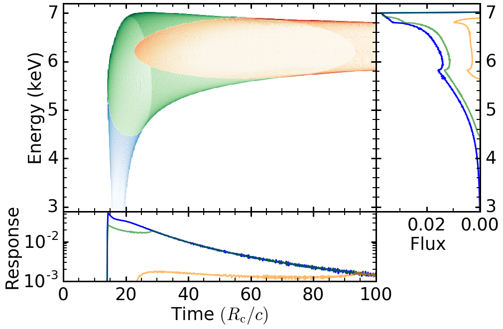
Figure 1: Central panel: Response function calculated for three different values of $r_{\rm in}$ of the disc: $1.2\,R_{\rm g}$ (blue), $10\,R_{\rm g}$ (green), and $50\,R_{\rm g}$ (red). For all three functions we consider a disc with $i=45\degree$ and $r_{\textmd{out}}=10^{6}\,R_{\rm g}$ illuminated by a flash of emission from a point like source at height $h=10\,r_{\rm g}$ above a black hole with spin $a=0.998$. Here $\mathscr{R}=\delta$ ($E-6.4$ keV). Right panel: Time integrated spectrum (i.e line profile). Bottom panel: Energy integrated flux (i.e. impulse response function).

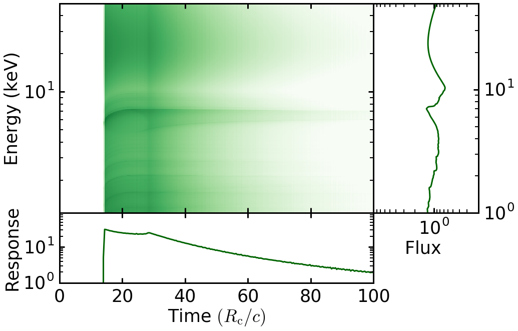
Figure 2: Central panel: Response function for a disc with $i=45\degree$, $r_{\textmd{in}}=10\,r_{\rm g}$, and $r_{\textmd{out}}=10^{6}\,R_{\rm g}$ illuminated by a flash from a point like source at height $h=10\,R_{\rm g}$ above a black hole with spin $a=0.998$. Here $\mathscr{R}$ is calculated using xillver with the parameters specified in the text. Right panel: Time integrated spectrum (i.e. energy spectrum). Bottom panel: energy integrated flux (i.e. impulse-response function).

3.3 Non-linear effects

In the previous Section we set $\beta=0$ as has been done in the literature. This means that the response function has been calculated assuming there are no phase lags associated with the continuum. However, neither AGN nor BHBs show any feature in the lag spectrum indicative of reverberation lags for frequencies below $\sim 300[M_{\odot}/M]\,{\rm Hz}$, with the lag spectrum instead dominated by featureless continuum lags (e.g. Kotov et al., 2001; Walton et al., 2013).

We model non-linear variation of the continuum spectrum with a variation of the power-law index; i.e. $\beta\neq 0$. We can see from Eq. 7 that the shape of the reflection spectrum now depends on time not just because of the response function, but also because it depends on the variable power-law index. Therefore Eq. 7 becomes non-linear for $\beta\neq 0$ and the simple transfer function formalism is not useful any more. We can, however, linearise. Following Kotov et al. (2001), we can Taylor expand the continuum spectrum to get

$$D\left(E,t\right)\simeq A\left(t\right)E^{-\Gamma}{\rm e}^{-\nicefrac{{E}}{{E_{\textmd{cut}}}}}\left[1+\beta\left(t\right)\ln E\right],$$ (10)

where we keep terms up to first order. We can take this further, and also Taylor expand the restframe reflection spectrum

$$\mathscr{R}\left(\Gamma-\beta\left(t\right)|E\right)\simeq\mathscr{R}\left(E|\Gamma\right)-\beta\left(t\right)\frac{\partial\mathscr{R}\left(E|\Gamma\right)}{\partial\Gamma},$$ (11)

where we compute $\partial\mathscr{R}/\partial\Gamma$ numerically. We explicitly test if it is reasonable to ignore higher order terms in the Taylor expansion in Appendix C. Since these expressions are both linear, we can once again employ the response function formalism using Eq. 11 to obtain a second response function (i.e. first order approximation whereas $w$ is the zero-order approximation):

$$w_{1}\left(E,t\right)= \int_{0}^{2\pi}\int_{r_{\rm in}}^{r_{\rm out}}K\left(r\right)g^{3}\left(r,\phi\right)\delta\left(t-\tau\left(r,\phi\right)\right)$$

$$\frac{\mathscr{R}\left(E/g(r,\phi)|\Gamma_{2}\right)-\mathscr{R}\left(E/g(r,\phi)|\Gamma_{1}\right)}{\Gamma_{2}-\Gamma_{1}}r\,{\rm d}r\,{\rm d}\phi,$$ (12)

where $\Gamma_{2}=\Gamma+\nicefrac{{\Delta\Gamma}}{{2}}$, $\Gamma_{1}=\Gamma-\nicefrac{{\Delta\Gamma}}{{2}}$ and $\Delta\Gamma$ sets the $\Gamma$ range where the variation of the restframe reflection spectrum as a function of $\Gamma$ is supposed to be linear. To keep the linearity even after the Fourier transform we define $B\left(t\right)=A\left(t\right)\beta\left(t\right)$. Since $\beta$ is arbitrary, we are free to introduce the more useful arbitrary variable $B$. The total emitted spectrum is simply $S(E,t)=D(E,t)+R(E,t)$ and its Fourier transform after the linearization can be written as

$$S\left(E,\nu\right)= A\left(\nu\right)\left[E^{-\Gamma}{\rm e}^{-\nicefrac{{E}}{{E_{\textmd{cut}}}}}+W\left(E,\nu\right)\right]$$

$$+ B\left(\nu\right)\left[E^{-\Gamma}{\rm e}^{-\nicefrac{{E}}{{E_{\textmd{cut}}}}}\ln E-W_{1}\left(E,\nu\right)\right].$$ (13)

Here, $W$ and $W_{1}$ are the transfer functions i.e. Fourier transform of the response function. Since the equation is linear in time the convolution converts into a multiplication in the frequency domain. We see the light-crossing lags are accounted for in Eq. 13 by the transfer functions, and the phase difference between $A$ and $B$ at each frequency introduces a continuum lag (the explicit derivation of Eq. 13 is in Appendix C).

We calculate the model complex covariance $G(E,\nu)$ by multiplying $S(E,\nu)$ (Eq. 13) with the complex conjugate of the Fourier transform $F(\nu)$ of an arbitrary reference band and dividing by its modulus. In the final expression of the complex covariance, we define the phase angles $\phi_{A}(\nu)=\arg[A(\nu)F^{*}(\nu)]$ and $\phi_{B}(\nu)=\arg[B(\nu)F^{*}(\nu)]$. We also define $\alpha(\nu)=\sqrt{\Delta}|A(\nu)|$ and $\gamma\left(\nu\right)=|B\left(\nu\right)|/|A\left(\nu\right)|$. The model complex covariance then becomes

$$G\left(E,\nu\right)=\alpha\left(\nu\right){\bigg{[}} {\rm e}^{i\phi_{A}\left(\nu\right)}\left[E^{-\Gamma}{\rm e}^{-E/E_{\rm cut}}+W\left(E,\nu\right)\right]+$$

$$\gamma\left(\nu\right)\, {\rm e}^{i\phi_{B}\left(\nu\right)}\left[E^{-\Gamma}{\rm e}^{-E/E_{\rm cut}}\ln E-W_{1}\left(E,\nu\right)\right]{\bigg{]}}.$$ (14)

Therefore, for each Fourier frequency considered, we model the continuum variation with four arbitrary parameters: $\alpha\left(\nu\right)$, $\gamma\left(\nu\right)$, $\phi_{A}\left(\nu\right)$ and $\phi_{B}\left(\nu\right)$. In the fits, these parameters are constrained by the data, but due to their arbitrary nature they do not constrain any of the physical parameters in our model. This does not affect our conclusions on the reflection parameters, which are constrained by the spectral correlations in the data described by our model. In principle, we could recover from these parameters the Fourier transform of $\beta\left(t\right)$. However, in practice this involves a deconvolution ($B(\nu)=A(\nu)\otimes\beta(\nu)$), which requires knowledge of the higher order variability properties of $A(\nu)$ and $B(\nu)$ (Körding & Falcke, 2004), which we do not constrain in our modelling. Since this is simply a mathematical model however, $\beta(t)$ is of no more physical interest than $\gamma(\nu)$, which can easily be constrained from data. To fit to the data Eq. 14 should be convolved with the instrument response matrix converting energies $E$ into channel numbers $I$. Therefore the final expression of the complex covariance model is

$$G(I,\nu)=\alpha(\nu)\left[{\rm e}^{i\phi_{A}(\nu)}Z(I,\nu)+\gamma(\nu){\rm e}^{i\phi_{B}(\nu)}Z_{1}(I,\nu)\right],$$ (15)

where $Z(I,\nu)$ and $Z_{1}(I,\nu)$ are respectively the convolution of $Z(E,\nu)=E^{-\Gamma}{\rm e}^{-E/E_{\rm cut}}+W(E,\nu)$ and $Z_{1}(E,\nu)=E^{-\Gamma}{\rm e}^{-E/E_{\rm cut}}\ln E-W_{1}(E,\nu)$ with the instrument response (see Appendix D for a demonstration that convolving the complex covariance with the response is equivalent to the actual process where we cross Fourier transforms of the convolved time series). Note that any additive/multiplicative model (such as line-of-sight absorption) should be applied before the convolution operation, as shown in the previous section and in Appendix A. We implement this by multiplying the real and imaginary part of the complex covariance with the absorption component directly and then convolving with the instrument response.

4 Model Parameter Exploration

In this Section we explore the parameter space of our model. Although in the following Section we will use real and imaginary parts of the complex covariance to fit to data, here we consider time lags and variability amplitude to explore the parameter space, since these are more intuitive. We can consider two main groups of model parameters: those that govern the response function and therefore the reverberation lags, and those that govern the continuum lags. Further parameters govern the restframe reflection spectrum, which we only briefly discuss but refer the interested reader to García et al. (2013a). Here, we first summarise the response function parameter dependencies and then concentrate on the continuum parameters. We then analyse the importance of accounting for the non-linear effects caused by fluctuations in the reflection energy spectrum.

4.1 Response function

The response function for a lamppost geometry depends on the height $h$ of the point source, the inclination angle $i$, the inner ($r_{\rm in}$) and the outer ($r_{\rm out}$) radius of the disc, the dimensionless spin parameter $a$ and the mass $M$ of the black hole. The parameter dependencies of such a response function have already been extensively explored in the literature (Cackett et al., 2014; Emmanoulopoulos et al., 2014). Therefore, here we only briefly explore the transfer function and refer the interested reader to previous papers for more detail. In Fig. 1, we show the response function assuming that the restframe reflection spectrum is simply a $\delta-$function iron line at $6.4$ keV. In Fig. 2 we instead use xillver to calculate the restframe reflection spectrum, setting the iron abundance $A_{\rm Fe}=1$, ionisation parameter $\log\xi=3.1$, cut-off energy of the incident power-law ${\rm E}_{\rm cut}=300$ keV and reflection fraction to $1.0$.

For both figures, we set $i=45^{\circ}$, $h=10$, $r_{\rm out}=10^{6}$ and $a=0.998$. Since we represent time in units of $R_{\rm g}/c$, Fig. 1 and Fig. 2 are independent of black hole mass. In Fig. 1 blue, green and orange represent an inner radius of $r_{\rm in}=1.2$, $10$ and $50$ respectively, while Fig. 2 shows the $r_{\rm in}=10$ case only. The central panels show the response function (with shades representing flux), the bottom panels show the impulse response function, and the right hand panel shows the time-averaged line profile. The time axis is defined such that the $\delta-$function flash in the continuum reaches the observer at a time of zero $R_{\rm g}/c$. After the continuum flash, the next photons to reach the observer are those that reflect from the front of the disc (as seen by the observer), at a radius that depends on $h$ and $i$. For $i=45^{\circ}$ and $h=10$ this radius is $10R_{\rm g}$. The initial sharp rise in the blue and green curves in Fig. 1 therefore occurs at the same time because the inner disc radius for both cases is $\leqslant 10R_{\rm g}$. The secondary peak in the impulse response function indicates when we see the first photons that reflect from the back of the disc. For a small $r_{\rm in}$, the broadest iron line is seen shortly after the continuum flash ($\sim 15R_{\rm g}/c$ for $r_{\rm in}=1.2$), whereas for $r_{\rm in}=50$ the iron line is initially narrow with its width peaking at $\sim 60R_{\rm g}/c$. This is because gravitational redshift is important for small radii, whereas Doppler broadening is dominant for larger radii. This can also be seen in the time-averaged line profile, which is smeared and skewed when the inner radius is small (e.g. blue line $r_{\rm in}$ = 1.2), while it has the characteristic double horn profile primarily due to Doppler shifts when the disc is far from the black hole (e.g. orange-red line $r_{\rm in}=50$ ). If we compare Fig. 1 with Fig. 2, we see the response functions and line profiles are very different because we used a different restframe reflection spectrum (we must compare the green lines because they have the same radius). In contrast, the restframe reflection spectrum makes little difference to the impulse response function, since this is the integral of the response function over all energies.

4.2 Continuum Variability

The continuum emission depends on the power-law index $\Gamma$ and cut-off energy $E_{\rm cut}$. We see from Eq. 14 that the continuum variations in a frequency range $\nu-\Delta/2$ to $\nu+\Delta/2$ are governed by the parameters $\alpha\left(\nu\right)$, $\gamma\left(\nu\right)$, $\phi_{A}\left(\nu\right)$ and $\phi_{B}\left(\nu\right)$. $\alpha(\nu)$ is simply a normalization of the variability amplitude for each frequency; i.e. it does not affect the phase lags at all and does not affect the energy dependence of the variability amplitude. Together, the other three parameters govern the energy and frequency dependence of the phase lags. We note that the four continuum variability parameters are not independent and one of them can in principle be derived from the other three using the definition of the reference band (see Appendix E). For the illustrative examples presented in this Section, we always use $\phi_{A}\left(\nu\right)=0$. This would, for example, be the case if there were no contributions from reflection and the reference band were chosen to be at $1$ keV.

To explore the continuum parameters, we set the black hole mass to $10M_{\odot}$ and fix the reflection parameters to those used for Fig. 2. In Figs. 3 and 4, we show the time lag (a) and variability amplitude (b) as a function of energy for a frequency range $1-2$ Hz. Here, amplitude is absolute amplitude in units of energy flux, not fractional amplitude. In Fig. 3, we fix $\phi_{B}\left(\nu\right)=0.2$ rad and different lines correspond to different values of $\gamma\left(\nu\right)$, which controls the amplitude of the power-law index oscillation. We see that increasing $\gamma\left(\nu\right)$ gives a larger absolute value of the lag. We can see from Eq. 14 that setting $\gamma\left(\nu\right)=0$ leads to no continuum lag at all. Fig. 3b shows that the amplitude spectrum becomes harder when $\gamma$ is increased. We can partially understand this by imagining a power-law pivoting around some energy $E_{0}$, such that the flux at $E_{0}$ remains constant and the variations for $E>E_{0}$ are in anti-phase with the variations for $E<E_{0}$. In this case, the variability amplitude increases with $|E-E_{0}|$. For a more realistic case in which the power-law index and the normalisation are varying (with a general phase difference between the variations in power-law index and normalisation), there can be no energy at which there is zero variability amplitude, but there will be an energy at which the amplitude reaches a minimum. The phase lags will also be anti-symmetric about this energy. We will call this the pivot energy, $E_{0}(\nu)$. Note that the pivot energy can be a function of frequency. Since the amplitude increases with energy in Fig. 3, the pivot energy for this example is $E_{0}(\nu)<1$ keV. It is worth noting however that extra complication occurs when a realistic spectral model including photoelectric absorption and a low energy cut-off are considered.

In Fig 4, we fix $\gamma(\nu)=0.1$ and vary $\phi_{B}(\nu)$. We see that increasing $\phi_{B}(\nu)$ also increases the lags. Panel (b) shows that increasing $\phi_{B}(\nu)$ makes the amplitude spectrum softer. This can be understood partially as the pivot energy increasing as $\phi_{B}(\nu)$ is increased. Figs. 3a and 4a show features around the iron line in the lag-energy spectrum, which are highlighted with a zoom-in. These result from the combination of reverberation lags and continuum lags, and also non-linear effects. The simplest effect comes from the reverberation lag simply being a different value from the continuum lag. In this case, the total energy spectrum is continuum plus reflection and so we expect a dip in the lags at the iron line if the reverberation lag is smaller than the continuum lag, and a peak for the opposite case, since the reflection dominates the energy spectrum at the iron line energy band. Non-linear effects further contribute to these features, with the variations in continuum power-law index causing changes in the shape of the disc reflection energy spectrum. This combination of effects leads to the dependence of the lag around the iron line on $\gamma(\nu)$ and $\phi_{B}(\nu)$ being subtle.

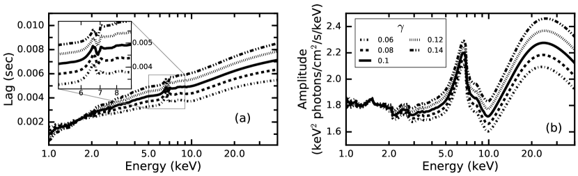
Figure 3: Predicted time lags (a) and absolute variability amplitude (b) as a function of energy for the frequency range $1-2\,{\rm Hz}$. For both panels, $\phi_{A}=0\,{\rm rad}$ and $\phi_{B}=0.2\,{\rm rad}$. The curves have different values of $\gamma$: $0.02$ solid line, $0.04$ dashed line, $0.06$ dotted dashed line, $0.08$ dotted line, $0.1$ dashed double dotted line. In both panels we use the parameters: $\Gamma=2$, $i=45\degree$, $r_{\textmd{in}}=10$, $r_{\textmd{out}}=10^{6}$, $h=10\,R_{\rm g}$, $a=0.998$, $M=10M_{\odot}$, $\log_{10}\xi=3.1$, $A_{\rm Fe}=1$ (respectively ionization and iron abundance in xillver).

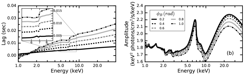
Figure 4: Predicted time lags (a) and absolute variability amplitude (b) as a function of energy for the frequency range $1-2\,{\rm Hz}$. For both panels, $\phi_{A}=0\,{\rm rad}$ and $\gamma=0.1$. The curves have different values of $\phi_{B}$: $0.2\,{\rm rad}$ solid line, $0.4\,{\rm rad}$ dashed line, $0.6\,{\rm rad}$ dotted dashed line, $0.8\,{\rm rad}$ dotted line, $1\,{\rm rad}$ dashed double dotted line. In both panels we use the parameters: $\Gamma=2$, $i=45\degree$, $r_{\textmd{in}}=10$, $r_{\textmd{out}}=10^{6}$, $h=10\,R_{\rm g}$, $a=0.998$, $M=10M_{\odot}$, $log_{10}\xi=3.1$, $A_{\rm Fe}=1$ (respectively ionization and iron abundance in xillver).

4.3 The Importance of Non-Linear Effects

Figure 5 shows the lag spectrum for different frequency ranges. The solid lines are produced with the complete model (both continuum and reverberation lags), while the dashed lines only include the reverberation lag (there is no variation of the continuum power-law index). For the dashed dotted lines, we instead calculate the continuum lags using our pivoting power-law model, but naively do not account for the variations in continuum power-law index when calculating the reflection spectrum (i.e. we set $W_{1}=0$ artificially). This allows us to assess the bias caused by not self-consistently accounting for the non-linear nature of the continuum variations. Here, we fix $\gamma(\nu)$, $\phi_{A}(\nu)$ and $\phi_{B}(\nu)$ to be constant with frequency (see the figure caption for all parameter values) and assume the same reflection parameters as those used for the previous sub-section. We see that, consistent with observational data, the continuum lags dominate over the reverberation lags for low frequencies, and the decrease of the continuum lag with frequency allows the reverberation lag to dominate at the highest frequencies. For low frequencies, the full model does differ quite significantly from the naive treatment, particularly below $\sim 2$ keV for which the full model predicts a steep break in the lag-energy spectrum. Therefore, ignoring non-linear effects could bias measurements of the reverberation lags. At high frequencies the models converge, since the lags are dominated by reverberation lags.

Fig. 6 shows the modulus of the complex covariance for a range of Fourier frequencies for the linear model (i.e. $\gamma=0$, meaning there are no continuum lags) and the full model ($\gamma=0.1$, meaning there are now continuum lags), represented respectively by the dots and the hatching. We see that, for both cases, the iron line feature is stronger for low frequencies (top lines) than for high frequencies (bottom lines). This is a result of the finite size of the reflector. Whereas the continuum can vary on arbitrarily short timescales, the fastest variability is washed out in the reflected emission by path length differences between rays that reflected from different parts of the disc (Gilfanov et al., 2000; Cackett et al., 2014). We also see that in terms of amplitude there is little difference between the two models, aside from the higher overall variability amplitude for the full model introduced by fluctuations in the continuum power-law index. The non-linear effects considered here therefore influence the predicted lags more than the amplitude and could therefore easily be missed when ignoring the lags.

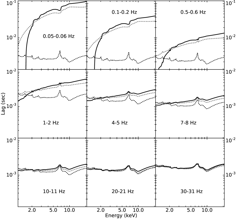
Figure 5: Time lag as a function of energy for different frequency ranges. The solid lines represent the lag calculated with the complete model: pivoting power-law in the continuum emission and contribution of reverberation. The dashed line is the lag only due to the reverberation (no pivoting power-law in the continuum emission). The dash-dotted line is the lag calculated considering the non-linear effect in the continuum emission (pivoting power-law) but naively ignoring this effect in the reverberation lag. The other parameters are $\phi_{A}=0\,{\rm rad}$, $\phi_{B}=0.2\,{\rm rad}$, $\Gamma=2$, $i=45\degree$, $r_{\textmd{in}}=10$, $r_{\textmd{out}}=10^{6}$, $h=10$, $a=0.998$, $M=10M_{\odot}$, $\log_{10}\xi=3.1$, $A_{\rm Fe}=1$.

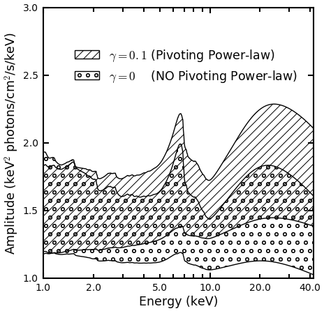
Figure 6: Covariance amplitude as a function of energy. The two regions represent frequency ranges from $0.02\,{\rm Hz}$ (the two highest curves) to $50\,{\rm Hz}$ (the two lowest curves). For the hatched region, we use the full model (pivoting power-law) and for the dotted region we do not include any continuum lags (NO pivoting model). All the parameters are equal to the ones in Fig. 5.

5 Example fits to Cygnus X-1 data

As a proof of principle of our method, we fit the complex covariance for a few hard state observations of Cygnus X-1 for multiple Fourier frequencies. The data analysis presented here is intended primarily to show the feasibility of jointly describing the non-linear continuum and resulting reflection variability using the methods outlined above. As the model does not contain a description of the relativistic light bending, the fit results should be interpreted with caution, in particular if they require a corona/disc geometry close to the black hole. Cygnus X-1 is one of the first black hole X-ray binaries observed and has been studied extensively during the past decades, in particular with the Rossi X-ray Timing Explorer (RXTE). Another motivation to select this source is the absence of strong low frequency QPOs, which are routinely seen in many other black hole X-ray binaries. Since there is good evidence that these signals are due to precession of the inner accretion flow (Ingram et al., 2016), or at least geometrical in origin (e.g. Heil et al., 2015; Motta et al., 2015; van den Eijnden et al., 2017), they complicate the situation somewhat. In particular, transfer modelling assumes a stationary geometry, and so it is convenient to avoid observations with strong QPOs. Following Revnivtsev et al. (1999); Kotov et al. (2001), we use RXTE observations P10238 recorded between March $26^{\rm th}$ and $31^{\rm st}$ 1996 by the proportional counter array (PCA). In all, this consists of seven observations. However, since the two first observations have a slightly different spectral slope we only consider these last five.

The timing data are in the ‘Generic Binned’ mode $B\_16{\rm ms}\_64{\rm M}\_0\_249$, which has $1/64$ sec time resolution in $64$ energy channels covering the whole PCA energy band. We apply standard RXTE good time selections (elevation greater than $10^{\circ}$ and offset less than $0.02^{\circ}$) and additionally select times when $5$ proportional counter units (PCUs) were switched on, using ftools from the heasoft 6.19 package. This gives a total exposure time of $56.2$ ks (after sorting into segments of contiguous data, the remaining useful exposure is $46.6$ ks). Following the procedure outlined in Section 2, we calculate the complex covariance for $8$ frequency ranges between $0.017$ and $32$ Hz. We assume unity coherence for this observation, which is a good assumption for the hard state of Cygnus X-1 (Nowak et al., 1999; Grinberg et al., 2014). The reference band is always $2.84-3.74$ keV and we consider the energy range $4-25$ keV for fitting. The choice of the reference band is discussed in Appendix E.

We use xspec version 12.9 (Arnaud, 1996) to fit real and imaginary parts of the complex covariance as a function of energy, simultaneously for all $8$ frequency ranges considered. We created an xspec local model for the complex covariance following the procedure explained in Section 3 using a cut off power-law for the continuum spectrum and xillver for the rest-frame reflection spectrum. We additionally fit the time-averaged energy spectrum with the DC component of the covariance model, meaning that we simultaneously fit accross $17$ spectra. The energy spectrum is computed adding the PCA standard $2$ data of the considered observations with the ftool addspec and adding in quadrature 0.1% systematic error .

For each of these 17 spectra, absorption is accounted for using the multiplicative model TBabs, assuming the abundances of Wilms et al. (2000). All parameters are tied to be the same for real and imaginary parts of a given frequency range. The parameters governing the continuum variations, $\phi_{A}(\nu)$, $\gamma(\nu)$ and $\phi_{B}(\nu)$, are allowed to vary freely with frequency. For the time-averaged spectrum, $\phi_{A}=\phi_{B}=\gamma=0$, whereas $\alpha(\nu)$ is a free normalisation parameter. All remaining model parameters are tied to be the same for all $17$ spectra. We fix the mass of the black hole to $14.8~{}M_{\odot}$ (Orosz et al., 2011). It is important to note that this analysis is sensitive to black hole mass and can therefore in future be used as a new method to estimate the mass. However, that is beyond the scope of this current paper.

We achieved a reduced $\chi^{2}=480.64/460$ with the physical parameters in Table 1. For the best fitting model, $r_{\rm in}$ is pegged at its lowest allowed value ($1.5$). This means that the model is not able to fully reproduce the shape and normalisation of the iron line simultaneously over the full range of frequencies considered. The source height is very close to the black hole ($2.4\pm 0.5$). As noted above, the values of these two parameters suggest caution in interpreting our results, as we explore a region close to the black hole without accounting for all the relevant physics (in particular, light bending).

To simplify the explored parameter space and to mimic an oblate geometry of the illuminating corona, we additionally tried tying the inner radius of the disc to be twice the height of the point source. In this case, the best fit has a reduced $\chi^{2}=484.43/461$, the height of the source is pegged to the lowest value. An F-test favours the first of the two models. The hydrogen column density is a free parameter in our best fitting model, with the best fit value giving a significantly better $\chi^{2}$ than fixing $N_{\rm h}=0.6\times 10^{22}{\rm cm}^{-2}$ following Gilfanov et al. (2000). From Table 1 it could be noted that our fit requires a strongly super-solar iron abundance $A_{\rm Fe}=4.0\pm 0.1$ as has previously been found in this source (e.g. Duro et al., 2016) and other BHBs (e.g. GX 339-4: García et al., 2015) . The high energy cut-off in our fit is compatible with what Wilms et al. (2006) found for the hard state of Cygnus X-1. We notice our value is slightly higher than their average, but the authors used a different model to fit the spectrum, for example accounting for the reflection with a Gaussian curve. We find a high reflection fraction compared to e.g. Parker et al. (2015); Basak et al. (2017). We expect this result to be highly biased by the absence of light bending in our model.

The best fitting continuum parameters are plotted in Fig. 7. Here, the black and blue points ($\phi_{A}$ and $\gamma$ respectively) correspond to y-axis scale on the left, while the red points ($\phi_{B}$) correspond to the y-axis scale on the right. $\phi_{A}$ and $\phi_{B}$ are in units of radians, whereas $\gamma$ is dimensionless. We see that all $3$ parameters reduce with frequency. Since our continuum lag model is simply empirical, the direct physical meaning of these parameters is not immediately clear. It is still interesting to compare the results in Fig. 7 with more physical models.

Figs. 8 and 9 show the data and best fitting model for $7$ of the $8$ frequency ranges considered (the lowest frequency range is very noisy). In Fig. 8, we show real (a) and imaginary (b) parts of the complex covariance, and plot the model with a higher energy resolution than the data for clarity. We additionally show fit residuals in the bottom panels. In Fig.9, we instead represent the data and model as time lag (a) and variability amplitude (b). In the lags, we see the characteristic dip at $\sim 6.4$ keV for both data and model, which becomes less prominent for higher frequencies. This occurs mainly because the continuum lags are greater than the reverberation lags, and so at the iron line the greater contribution from reflection dilutes the overall time lag. For higher frequencies, the difference between continuum and reverberation lags reduces and so the dip becomes less prominent. For even higher frequencies, we expect to see an emission-like feature at the iron line, but unfortunately the maximum possible Nyquist frequency for this data mode is $32$ Hz. For the amplitude, we see the iron line becomes less prominent for higher frequencies, which is due to the finite size of the reflector as discussed in Section 4.

Fig. 8 shows that there are some systematic residuals in the real part of the complex covariance around the iron line. This seems to be because the amplitude of the iron line reduces more steeply with frequency in the data compared with the model. In the model, the accretion geometry (i.e. the source height and disc inner radius) sets both the frequency dependence of the iron line amplitude and the width of the iron line. For a smaller inner disc radius, the iron line is broader and the variability amplitude of reflection drops-off less steeply with frequency. Therefore, it appears that our small best-fitting inner radius of $r_{\rm in}\approx 1.5$ reproduces the broad iron line seen in the complex covariance and time-averaged spectrum, but predicts a slower drop-off in reflection variability amplitude with frequency than is observed. Since the data constrain the broadness of the iron line at all frequencies better than they constrain the drop off of the line amplitude at high frequencies, our fit returns a small value for inner radius. These residuals may be fixed in future by considering light bending, since this would give $1$) longer reverberation lags for a given disc inner radius due to longer path lengths of rays close to the black hole, and $2$) a broader iron line for a given disc inner radius due to the steeper emissivity profile resulting from focusing of rays close to the black hole.

Table 1: Best fitting disc parameters obtained from our simultaneous fit to the complex covariance in $8$ frequency ranges ($0.017-32Hz$) and the time-average spectrum. The $\chi^{2}$ is $480.64$ with $460$ degrees of freedom. We report 1 $\sigma$ errors for each parameter value.

$N_{\rm h}$ $\left(10^{22}\,\,{\rm cm}^{-2}\right)$	$\Gamma$	h $(R_{\rm g})$	$r_{\rm in}\,(R_{\rm g})^{a}$	Incl $({\rm deg})$	$A_{\rm Fe}$	$E_{\rm cut}$ (keV)	$\log\xi$	Reflection Fractionb
$0.2\pm^{0.2}_{0.1}$	$1.603\pm^{0.004}_{0.003}$	$2.4\pm^{0.5}_{0.5}$	$1.5\pm^{0.6}_{0}$	$35.7\pm^{1.2}_{1.3}$	$4.0\pm^{0.1}_{0.1}$	$241\pm^{10}_{5}$	$3.08\pm^{0.01}_{0.01}$	$-0.93\pm^{0.02}_{0.02}$

• The parameter is pegged at its minimum allowed value.

• In xillver a negative reflection fractions means the model represents only the reflection spectrum without the continuum.

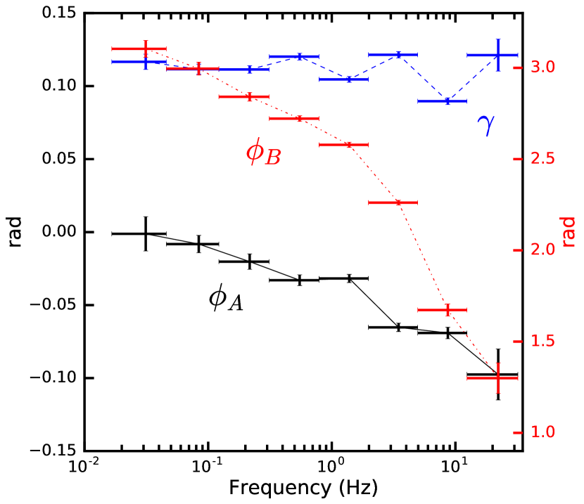
Figure 7: Continuum variability parameters as function of Fourier frequency. The black solid and blue dashed curves refer to the left y-axis, while the red dotted curve refers to the right y-axis. The x-errorbars represent the range of frequency used to fit the complex covariance as a function of energy. The points with the same frequency range are computed from the same fit.

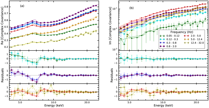
Figure 8: Fit of the real (a) and imaginary (b) part of Cygnus X-1 complex covariance spectrum for different Fourier frequency ranges. The dots are the data, the solid line is the model with a better energy resolution. Both the bottom panels show the data minus the folded model in units of normalised counts per second per keV (command residuals in xspec). The residuals around the iron line are discussed in the text.

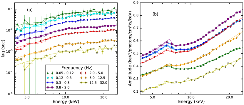
Figure 9: Lag (a) and variability amplitude (b) as a function of energy for different Fourier frequency ranges. Both data and model have been derived from the fit of real and imaginary part of the complex covariance spectrum (Fig. 8).

6 Discussion

In this paper we have introduced a formalism to fully utilize X-ray reverberation mapping as a tool to measure the geometry of accreting black holes, and ultimately to provide a new means of measuring black hole mass and inner radius of the disc. The main innovation is that we fit a reverberation model that considers phase lags and variability amplitude jointly for a wide range of Fourier frequencies for the first time. In order to do this, we introduce the complex covariance, and show that it is statistically more convenient to fit for the real and imaginary parts of the complex covariance than fitting directly for the amplitude and phase lags, which has led to some previous inaccuracies in the literature (it is still possible to compute the amplitude and phase lags, which are more physically intuitive, and compare them with other works). In order to fit for the full range of Fourier frequencies (determined by the duration and time resolution of the observation) we need to account for the continuum lags that dominate at low frequencies. We introduce a simple variation in the slope of the continuum emission (pivoting power-law model), and use a Taylor expansion to calculate the model analytically whilst still accounting for the variations in disc reflection spectrum shape caused by fluctuations in the illuminating power-law index. As noted by Kotov et al. (2001); Körding & Falcke (2004), a pivoting power-law model is fairly attractive, since it naturally produces time lags with a log-linear energy dependence, as is regularly observed.

The continuum lags are often assumed to result from propagating mass accretion rate fluctuations, with perturbations far from the black hole propagating inwards and modulating new fluctuations generated closer to the black hole (Lyubarskii, 1997; Kotov et al., 2001; Arévalo & Uttley, 2006). We note that, if the power-law emitting region is small compared with the disc inner radius, our adopted lamppost geometry still provides a good approximation to propagating fluctuations models. However, our treatment is at odds with sandwich models that consider propagation in a coronal layer above and below the disc. It could be that propagating fluctuations cause fluctuations in power-law index, through, for example, accretion rate fluctuations in the disc giving rise to fluctuations in the luminosity of seed photons (Uttley et al., 2014, Uttley & Malzac in prep). The fluctuations in power-law index could also result from fluctuations in electron temperature, seed photon luminosity and/or optical depth of the Comptonising region.

A few authors have made progress on integrating a propagating fluctuation model with reverberation modelling. Wilkins & Fabian (2013) consider fluctuations propagating through the corona with different geometries, and calculate reflection from each region of the corona. This is perhaps the most physically self-consistent treatment in the literature, but requires many response functions and so is computationally expensive. It will therefore be challenging to attempt the multi-frequency fits that we present here with such a model. Chainakun et al. (2016) and Chainakun & Young (2017) instead explore a ‘two blobs’ model, consisting of two lamppost sources with different heights and different intrinsic spectra, with the propagation time between the two sources set as a model parameter. This is of comparable simplicity to our treatment, indeed both of our formalisms require only two response functions. It therefore should be possible to also fit this model for the full range of Fourier frequencies, and comparison of our two different formalisms may provide information on the physical origin of the continuum lags.

An interesting result we find here is that the low frequency lag spectrum is predicted to dip dramatically at $\sim 2$ keV (see top left of Fig. 5), which Uttley et al. (2011) see for GX 339-4. They attribute it to fluctuations propagating in from the disc, which could well be the case because of the shape of the covariance spectrum, but it is interesting to note that we naturally expect this dip at $\sim 2$ keV without any disc component. This is true only if we account for the non-linear effects, indicating that ignoring them could bias the results. We note, however, that the introduction of a low energy cut-off in the continuum spectrum of our model could modify the lags at such low frequency.

Since the model is analytic, fits to data for many frequencies are feasible without prohibitive computational expense. We fit hard state Cygnus X-1 data, and find an unphysically low value for the disc inner radius in our best-fit. Moreover the fit shows some residuals in the iron line energy range of the real part of the covariance spectrum for low frequencies. In the data, the line appears to be broad, both in the time-averaged spectrum and for non-zero Fourier frequencies, implying a small disk inner radius. However, the variability amplitude of the reflection signal drops off with frequency, which in itself favours a fairly large disk inner radius (Gilfanov et al., 2000). It is this tension that is behind the residuals seen in Fig. 8. However, the transfer function we used to model reflection in this illustrative fit is over-simplified. In particular, including light bending should go some way to improving the fit as it both increases the light travel time of reflected X-rays and focuses them to the inner regions of the disk. In any case, the inclusion of light bending will dramatically alter the model for our best fitting parameters, and so our results from Section 5 should be seen only as a proof of principle of the method, with further insight delayed until all GR effects are included in the analysis.

The value of the disk inner radius of Cygnus X-1 in the hard state has long been a subject of debate in the literature. For example, reflection modelling of the same NuSTAR dataset gives values of $r_{\rm in}$ ranging from $\simeq 1.3R_{\rm g}$ (Parker et al., 2015) to $\simeq 13-20R_{\rm g}$ (Basak et al., 2017), depending on assumptions about the continuum. Rapisarda et al. (2017) obtain a similar result for the inner radius $\sim 20~{}R_{\rm g}$ fitting a propagating fluctuations model to a hard state observation of Cygnus X-1, although they did not account for the reverberation effects on the lags. We also note that the high resolution data used by Parker et al. (2015) reveal absorption features around the iron line which would not be detectable with RXTE data. Since the absorption properties of Cygnus X-1 depend on the binary orbital phase (likely due to the wind from the companion; Grinberg et al., 2015), it is not clear if such absorption features affect our data. Here, we fixed the black hole mass in our fits but note that this can be left as a free parameter in future. We also note that the same model can be used for AGN, and is also sensitive to black hole mass in this case.

Aside from including light bending, a number of other improvements can be made to our method. More realistic geometries than the lamppost model can be explored in future, albeit with the trade-off of extra complexity increasing computational expense. Our model is designed such that any transfer function can be ported into our formalism, allowing flexibility. It will also be fairly simple to include variations in cut-off energy and ionisation parameter. As with power-law index variations considered here, this can be done using a Taylor expansion, and so will not add prohibitively to computational cost. Finally, we have assumed that reflection is instantaneous, as is routinely assumed in the literature. In reality, the reflected flux will take some finite time to increase when the illuminating flux increases (on top of the light-crossing time). García et al. (2013b) showed, albeit with a very simple model, that the reflection spectrum for a stellar-mass black hole should indeed respond very quickly ($\sim 1$ ns) to a rise in the illuminating flux, but the response to a drop in illuminating flux could take as long as $\sim 1$ ms for a very low disc density. The different timescales occur because the rise time depends on photoionisation, but the fall time depends on recombination. Therefore, this response time may be relevant for reverberation mapping.

7 Conclusions

We developed a formalism for X-ray reverberation mapping of accreting black holes that enables characterisation of the full range of cross-spectral properties for a wide range of Fourier frequencies. We empirically model the continuum lags that dominate at low Fourier frequencies, and self-consistently account for the effect of the continuum lags on the reverberation signal. We point out some of previous inaccuracies in the literature associated with fitting models to the observed energy dependent phase lag and variability amplitude, and employ real and imaginary parts of the complex covariance to easily circumvent such problems. As a proof of principle, we have fitted our model to an RXTE observation of Cygnus X-1 in the hard state. We assume an on-axis lamppost geometry, and obtain a fit with reasonable $\chi^{2}$, albeit with systematic residuals around the iron line that would likely be improved by the inclusion of light bending in the reflection model. We also note that more realistic geometries will impact these results. Although here we fixed the black hole mass in our fits to $14.8~{}M_{\odot}$ (following Orosz et al., 2011), we note that the model is sensitive to the black hole mass. This optimised model for X-ray reverberation mapping using the information of the cross variability for a wide range of Fourier frequencies can therefore be used in future as a new way to measure the mass of stellar-mass and supermassive black holes.

Appendix A Complex covariance analysis

Analysing real and imaginary parts means that any linearity of the signal in the time domain is preserved in the frequency domain. This is not the case for amplitude and phase. Here we consider two simple explicit examples to illustrate the superiority of considering real and imaginary parts instead of amplitude and phase. The first concerns the response matrix of the instrument and the second concerns scenarios when multiple variable spectral components are present. We assume unity coherence and infinite ensemble averaging, allowing us to drop angle the brackets notation.

A.1 Instrument Response

It is often assumed that the instrument response can be applied to the cross-spectral amplitude (or covariance/rms), giving

$$|G_{\rm o}\left(I,\nu\right)|=\int_{0}^{+\infty}R_{\rm t}\left(E,I\right)|G\left(E,\nu\right)|dE$$ (16)

where $G_{\rm o}\left(I,\nu\right)$ is the observed complex covariance in the specific energy channel $I$ and $R_{\rm t}\left(I,E\right)$ is the instrument response. Here, $G\left(E,\nu\right)$ is in units of photons per second per ${\rm cm}^{2}$ per keV, and $G_{\rm o}$ is in units of counts per second. However, this expression is not correct in general. The correct expression is

$$G\left(I,\nu\right)=\int_{0}^{+\infty}R_{\rm t}\left(E,I\right)\,G\left(E,\nu\right)dE.$$ (17)

The amplitude of the complex covariance for channel $I$ is then

$$|G_{\rm o}\left(I,\nu\right)|=\sqrt{\begin{aligned} &\left[\int_{0}^{+\infty}R_{\rm t}\left(E,I\right){\rm Re}\left[G\left(E,\nu\right)\right]dE\right]^{2}+\\ &\left[\int_{0}^{+\infty}R_{\rm t}\left(E,I\right){\rm Im}\left[G\left(E,\nu\right)\right]dE\right]^{2}\end{aligned}}.$$ (18)

where ${\rm Re}$ and ${\rm Im}$ respectively denote the real and the imaginary part. For $Re\left[G\left(E,\nu\right)\right]\neq 0$ and $Im\left[G\left(E,\nu\right)\right]\neq 0$, Eq. 16 is therefore incorrect. In the special case where $Re\left[G\left(E,\nu\right)\right]=0$ or $Im\left[G\left(E,\nu\right)\right]=0$, Eq. 18 does reduce to Eq. 16.

Since the observed phase lags are often fairly small, Eq. 16 is, in practice, often fairly close to true. However, using our formalism of treating real and imaginary parts separately introduces no mathematical errors, and is no more difficult to implement than considering the amplitude and the phase. It is clear the instrument response cannot be applied to the phase in a manner analogous to Eq. 16.

A.2 Multiple Components Fitting

Consider a signal $s_{1}\left(E,t\right)=p\left(E\right)a\left(t\right)$ and another signal $s_{2}=q\left(E\right)b\left(t\right)$, with Fourier transforms $p\left(E\right)A\left(\nu\right)$ and $q\left(E\right)B\left(\nu\right)$. Using Eq. 1 it follows from the linearity of the Fourier transform that the cross-spectrum of $s_{1}\left(E,t\right)+s_{2}\left(E,t\right)$ is

$$C\left(E,\nu\right)=A\left(\nu\right)p\left(E\right)F^{*}\left(\nu\right)+B\left(\nu\right)q\left(E\right)F^{*}\left(\nu\right);$$ (19)

i.e. simply the sum of the two individual cross-spectra. However, this linearity is lost for the amplitude and the phase lag. Setting, for simplicity, the amplitude and phase of the reference band to $|F\left(E_{\rm r}\nu\right)|=1$ and $\phi_{F}\left(\nu\right)=0$ respectively, the amplitude and phase lag of the cross-spectrum are

$$|C\left(E,\nu\right)|= \sqrt{p^{2}|A|^{2}+q^{2}|B|^{2}+2pq{\rm Re}\left[A\,B^{*}\right]}$$

$$\tan\phi_{C}\left(E,\nu\right)= \left[\frac{p\,{\rm Im}\left[A\right]+q\,{\rm Im}\left[B\right]}{p\,{\rm Re}\left[A\right]+q\,{\rm Re}\left[B\right]}\right],$$ (20)

In both expressions we have dropped the energy and frequency dependence of the components so as not to weigh the notation. We see that the expression of the amplitude has a cross term that would not appear if we simply added the amplitude of the two components. The exception is if the two components are in phase with each other, since in this case the amplitude of two vectors added in the complex plane is equal to the sum of the two amplitudes. Kotov et al. (2001) considered the case where the contribution of one component (e.g. $q(E)B(\nu)$) is small compared to the total spectrum ($q<<p$), in that case a binomial expansion gives

$$|C\left(E,\nu\right)|\simeq p\,|A|\sqrt{1+2\frac{q\,Re\left[A\,B^{*}\right]}{p\,|A|^{2}}}$$

$$\simeq p\,|A|+q\,\frac{Re\left[A\,B\right]}{|A|}=p|A|+q|B|\cos\phi_{AB},$$ (21)

where $\phi_{\rm AB}$ is the phase difference between $A$ and $B$. Therefore, the contribution from the cross-terms in this case is small, but the normalisation of the second component is modified by a factor $\cos\phi_{AB}$. From Eq. 20, it is clear that summing lags of two components is not appropriate.

Appendix B Response function

Eq. 7 in the text refers to emission from a specific patch of the accretion disc area. If the we consider flat space the area is expressed by $r\,dr\,d\phi$ and the total observed reflection spectrum varying in time is calculated by integrating the specific flux over the entire disc

$$R\left(E,t\right)=\int_{r_{\textmd{in}}}^{r_{\textmd{out}}}\int_{0}^{2\pi}K(r)g^{3}A\left(t-\tau\right)\mathscr{R}\left(E/g\right)r\,dr\,d\phi,$$ (22)

where we have not specified the $r$ and $\phi$ dependence of $g$ and $\tau$ for brevity. As defined in the main text, $E$ is the observed energy and $\mathscr{R}$ is the restframe reflection spectrum. The factor $K\left(r\right)$ accounts for geometrical dilution of radiation from the the point source incident on the disc patch, and is given by

$$K\left(r\right)=\varepsilon\left(r\right)\frac{\cos i}{D^{2}}=\frac{h\,\cos i}{\left(h^{2}+r^{2}\right)^{\nicefrac{{3}}{{2}}}\,D^{2}}.$$ (23)

The blue shift $g\left(r,\phi\right)$ is given by

$$g\left(r,\phi\right)=\frac{\sqrt{-g_{tt}-2g_{t\phi}\omega-g_{\phi\phi}\omega^{2}}}{1+\omega r\sin\phi\sin i},$$ (24)

where $\omega=1/\left(r^{3/2}+a\right)$ is the angular velocity in the dimensionless units, and we have again ignored light-bending (see Ingram et al., 2015, 2017). Finally light-crossing lag, $\tau\left(r,\phi\right)$, (i.e. the difference between the path of the light traveling directly from the point source to the observer and the light reflecting from the disc divided over the speed of light $\tau=l/c$) is given by

$$\tau c=\sqrt{r^{2}+h^{2}}-r\sin i\cos\phi+h\cos i,$$ (25)

when light-bending is ignored.

Appendix C Linearization

Taylor expanding Eq 7 around $\beta=0$ gives

$$dR\left(r,\phi|E,t\right)\simeq A\left[t-\tau(r,\phi)\right]{\bigg{[}}\mathscr{R}\left(E/g(r,\phi)|\Gamma\right)-\beta\left(t-\tau(r,\phi)\right)$$

$$\frac{\partial\mathscr{R}}{\partial\Gamma}\left(E/g\left(r,\phi\right),\Gamma\right){\bigg{]}}K(r)\,g^{3}\left(r,\phi\right)r\,{\rm d}r\,{\rm d}\phi.$$ (26)

Setting $B\left(t\right)\equiv A\left(t\right)\beta\left(t\right)$, the reflected flux integrated over the entire disc is

$$R\left(E,t\right)\simeq \int_{t^{\prime}=0}^{t^{\prime}=\infty}\int_{\phi=0}^{\phi=2\pi}\int_{r=r_{\rm in}}^{r_{\rm out}}A\left(t^{\prime}\right)\delta\left(t-\tau-t^{\prime}\right)$$

$$\mathscr{R}\left(E/g\left(r,\phi\right)|\Gamma\right)K\left(r\right)g^{3}\left(r,\phi\right)r\,{\rm d}r\,{\rm d}\phi\,dt^{\prime}-$$

$$\int_{t^{\prime}=0}^{t^{\prime}=\infty}\int_{\phi=0}^{\phi=2\pi}\int_{r=r_{\rm in}}^{r_{\rm out}}A\left(t^{\prime}\right)\delta\left(t-\tau-t^{\prime}\right)$$

$$\frac{\partial\mathscr{R}}{\partial\Gamma}\left(E/g\left(r,\phi\right)|\Gamma\right)K\left(r\right)g^{3}\left(r,\phi\right)r\,{\rm d}r\,{\rm d}\phi\,dt^{\prime}.$$ (27)

From the definition of a convolution

$$A(t)\otimes z\left(E,t\right)\equiv\int_{0}^{\infty}z\left(E,t-t^{\prime}\right)A(t^{\prime})\,{\rm d}t^{\prime},$$ (28)

where $z\left(E,t\right)$ is an arbitrary function of energy and time. We can simplify to

$$R\left(E,t\right)=A(t)\otimes w\left(E,t\right)-B(t)\otimes w_{1}\left(E,t\right),$$ (29)

where $w\left(E,t\right)$ and $w_{1}\left(E,t\right)$ are defined in the main text. For the continuum, it is clear from Eq. 10 that

$$D\left(E,t\right)\simeq\left[A\left(t\right)+B\left(t\right)\ln E\right]E^{-\Gamma}{\rm e}^{-E/E_{\rm cut}}.$$ (30)

Summing direct and reflected components, and using the convolution theorem gives Eq. 13 in the main text. The transfer functions can be written analytically as

$$W\left(E,\nu\right)=\int_{r_{\rm in}}^{r_{\rm out}}\int_{0}^{2\pi}{\rm e}^{i2\pi\nu\tau}K(r)g^{3}\mathscr{R}\left(E/g|\Gamma\right)r\,{\rm d}r\,{\rm d}\phi$$

$$W_{1}\left(E,\nu\right)=\int_{r_{\rm in}}^{r_{\rm out}}\int_{0}^{2\pi}{\rm e}^{i2\pi\nu\tau}K(r)g^{3}\frac{\partial\mathscr{R}}{\partial\Gamma}\left(E/g|\Gamma\right)r\,{\rm d}r\,{\rm d}\phi,$$ (31)

where we neglected the $r$ and $\phi$ dependency of $g$ and $\tau$ for brevity. In our code, we first calculate transfer functions for $\mathscr{R}=\delta\left(E-1{\rm keV}\right)$ and $\frac{\partial\mathscr{R}}{\partial\Gamma}=\delta\left(E-1{\rm keV}\right)$ and then perform convolution operations in the energy variable with $\mathscr{R}\left(E|\Gamma\right)$ and $\frac{\partial\mathscr{R}}{\partial\Gamma}\left(E|\Gamma\right)$ for obtaining $W$ and $W_{1}$ respectively.

We checked under which conditions the linearisation of both the continuum and reflection expression is valid. Fig. 10 shows the lag-energy spectrum at $2.5$ Hz calculated in the time domain without Taylor expanding either the continuum or the reflection expressions (solid lines) and analytically using first order linearisation (dashed lines). We used a single frequency sine wave as input of the exact calculation of the lags, i.e. $A\left(t\right)\propto 1+\sin\left(2\pi\nu t-\phi_{\rm A}\right)$ and $B\left(t\right)\propto\sin\left(2\pi\nu t-\phi_{\rm B}\right)$. The top panel (a) shows that for a reasonable choice of $\Delta\Gamma$ and a value of $\gamma$ similar to what we found from the fitting procedure the two curves match. However, if we decided to increase one of the two parameters (central and bottom panel) the Taylor expansion is less accurate.

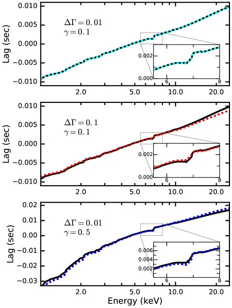
Figure 10: Predicted time lags as a function of energy for $2.5{\rm Hz}$. For all the panels the solid curves are the exact prediction (made in the time domain without Taylor expansion) and the dashed curves are calculated using the Eq. 10 and 11 (first-order Taylor expansion). For all the panels, $\phi_{A}=0\,{\rm rad}$ and $\phi_{B}=0.2\,{\rm rad}$. In all panels we use the parameters: $\Gamma=2$, $i=30\degree$, $r_{\textmd{in}}=10$, $r_{\textmd{out}}=100$, $h=10\,R_{\rm g}$, $a=0.998$, $M=10M_{\odot}$, $\log_{10}\xi=3.1$, $A_{\rm Fe}=1$

Appendix D Convolution of the theoretical model with the instrument response

Our model for the Fourier transform of the spectrum, $S(E,\nu)$, is given by Eq. 13 in the main text. Setting $Z(E,\nu)=E^{-\Gamma}{\rm e}^{-E/E_{\rm cut}}+W(E,\nu)$ and $Z_{1}(E,\nu)=E^{-\Gamma}{\rm e}^{-E/E_{\rm cut}}\ln E-W_{1}(E,\nu)$ gives the simplified form

$$S(E,\nu)=A(\nu)Z(E,\nu)+B(\nu)Z_{1}(E,\nu).$$ (32)

Note that $Z$ and $Z_{1}$ are complex in general, due to the phase lags introduced by the transfer functions $W$ and $W_{1}$. Convolving this around the instrument response (using the same procedure explained in Eq. 17 in Appendix A) gives the Fourier transform of the observed spectrum

$$S(I,\nu)=A(\nu)Z(I,\nu)+B(\nu)Z_{1}(I,\nu),$$ (33)

where $I$ indicates the $I^{\rm th}$ energy channel. The Fourier transform of reference band flux is $F(\nu)$, and therefore our model for the complex covariance of the $I^{\rm th}$ energy channel is

$$G(I,\nu)=\frac{A(\nu)F^{*}(\nu)Z(I,\nu)+B(\nu)F^{*}(\nu)Z_{1}(I,\nu)}{|F(\nu)|}.$$ (34)

To simplify further, we can simply set

$$\alpha(\nu){\rm e}^{i\phi_{A}(\nu)} =\frac{A(\nu)F^{*}(\nu)}{|F(\nu)|}$$ (35)

$$\alpha(\nu)\gamma(\nu){\rm e}^{i\phi_{B}(\nu)} =\frac{B(\nu)F^{*}(\nu)}{|F(\nu)|}$$ (36)

to get

$$G(I,\nu)=\alpha(\nu)\left[{\rm e}^{i\phi_{A}(\nu)}Z(I,\nu)+\gamma(\nu){\rm e}^{i\phi_{B}(\nu)}Z_{1}(I,\nu)\right].$$ (37)

This expression is identical to Eq. 15 that we derived in the main text convolving the final complex covariance model (Eq. 14) with the instrument response.

Appendix E Reference band

Following Revnivtsev et al. (1999) and Gilfanov et al. (2000), who analysed the observations considered here, we choose channels $5-7$ ($2.84-3.74$ keV) as our reference band. This choice is motivated by these channels having high count rates and being disjunct from the ‘science’ channels (and thus ensuring statistical independence between the reference band and all of the science channels). Moreover the $2.84-3.74$ keV range does not contain any of the reflection features that we are interested in observing. When the complex covariance is calculated (for the data) in the reference band energy range, the imaginary part is identically zero because the complex covariance of the reference band with itself has zero phase by definition. This could, in principle, impose an additional constraint that involves all the continuum parameters of the model:

$$\sum_{I=I_{1}}^{I_{2}}{\rm Im}\left[G(I,\nu)\right]=0,$$ (38)

where $I$ indicates the $I^{\rm th}$ energy channel, $I_{1}$ to $I_{2}$ set the reference band channel range and $G(I,\nu)$ is defined in Eq. 17. In our case it is not possible to apply this extra condition because the available instrument response $R^{\prime}_{\rm t}(E,I)$ is poorly calibrated in the energy range of the reference band, while the relation between $G(E,\nu)$ and $G(I,\nu)$ is of course always defined by the true instrument response $R_{\rm t}(E,I)$. A mathematical way of looking at it is that we construct a model for the Fourier frequency dependent spectrum $S(E,\nu)$, which we cross with the Fourier transform of a model reference band, $F(\nu)$, to get the predicted complex covariance

$$G(E,\nu)=\frac{S(E,\nu)F^{*}(\nu)}{|F(\nu)|}.$$ (39)

If we had a response matrix that were well calibrated for the reference band energy channels, we could self-consistently calculate the reference band Fourier transform from our spectral model

$$F(\nu)=\int_{0}^{\infty}\sum_{I_{1}}^{I_{2}}R_{t}(E,I)S(E,\nu)dE.$$ (40)

However, we do not know the true response $R_{\rm t}(E,I)$, and so we simply leave the phase angle of the unity magnitude complex number $F(\nu)/|F(\nu)|$ as a model parameter that gets swallowed up into the definition of the parameters $\phi_{A}(\nu)$ and $\phi_{B}(\nu)$. In order to calculate $G(I,\nu)$ to fit to the data, we convolve $G(E,\nu)$ with the available response $R^{\prime}_{t}(E,I)$. This response is actually well calibrated in the range where we fit it to the data, so assuming the model is correct we obtain the correct values for the fit parameters and hence correctly recover $G(E,\nu)$. If we could convolve this $G(E,\nu)$ with the true response $R_{\rm t}(E,I)$, the $G(I,\nu)$ obtained from this operation would satisfy condition 38. However, if we convolve $G(E,\nu)$ with the available response $R^{\prime}_{\rm t}(E,I)$ which is poorly calibrated and hence differs from $R_{\rm t}(E,I)$ between $I_{1}$ and $I_{2}$, we obtain

$$\frac{\int_{0}^{\infty}\sum_{I_{1}}^{I_{2}}R^{\prime}_{\rm t}(E,I)S(E,\nu)dE\,\,F^{*}(\nu)}{|F(\nu)|}=\frac{F^{\prime}(\nu)F^{*}(\nu)}{|F(\nu)|},$$ (41)

whose imaginary part is not identically zero. For this reason, using the available response, condition 38 is not expected to apply to our chosen reference band. Indeed, when we perform this experiment this turns out to be the case, although the discrepancy is not very large, indicating the calibration, while poor, is still passable even in the energy range of the reference band. It is worth noting that the poor calibration of the reference band does not affect our measurements of $G(E,\nu)$. Since we divide through by the modulus of $F(\nu)$, all that is affected is the phase of our reference band model $F(\nu)$. At any given frequency this only introduces a phase offset that is the same at each energy, not affecting the physically meaningful phase differences between energy bands. In the absence of a physical time series model, however, the phase differences between Fourier frequencies in a given energy band can not be used to constrain the physical parameters.

References

- Arévalo & Uttley (2006) Arévalo P., Uttley P., 2006, MNRAS, 367, 801
- Arnaud (1996) Arnaud K. A., 1996, in Jacoby G. H., Barnes J., eds, Astronomical Society of the Pacific Conference Series Vol. 101, Astronomical Data Analysis Software and Systems V. p. 17
- Axelsson et al. (2013) Axelsson M., Hjalmarsdotter L., Done C., 2013, MNRAS, 431, 1987
- Basak et al. (2017) Basak R., Zdziarski A. A., Parker M., Islam N., 2017, preprint, (arXiv:1705.06638)
- Cackett et al. (2014) Cackett E. M., Zoghbi A., Reynolds C., Fabian A. C., Kara E., Uttley P., Wilkins D. R., 2014, MNRAS, 438, 2980
- Campana & Stella (1995) Campana S., Stella L., 1995, MNRAS, 272, 585
- Chainakun & Young (2017) Chainakun P., Young A. J., 2017, MNRAS, 465, 3965
- Chainakun et al. (2016) Chainakun P., Young A. J., Kara E., 2016, MNRAS, 460, 3076
- De Marco & Ponti (2016) De Marco B., Ponti G., 2016, ApJ, 826, 70
- De Marco et al. (2015) De Marco B., Ponti G., Muñoz-Darias T., Nandra K., 2015, ApJ, 814, 50
- De Marco et al. (2017) De Marco B., et al., 2017, MNRAS, 471, 1475
- Done et al. (2012) Done C., Davis S. W., Jin C., Blaes O., Ward M., 2012, MNRAS, 420, 1848
- Duro et al. (2016) Duro R., et al., 2016, A&A, 589, A14
- Eardley et al. (1975) Eardley D. M., Lightman A. P., Shapiro S. L., 1975, ApJ, 199, L153
- Emmanoulopoulos et al. (2014) Emmanoulopoulos D., Papadakis I. E., Dovčiak M., McHardy I. M., 2014, MNRAS, 439, 3931
- Fabian et al. (1989) Fabian A. C., Rees M. J., Stella L., White N. E., 1989, MNRAS, 238, 729
- Fabian et al. (2009) Fabian A. C., et al., 2009, Nature, 459, 540
- García & Kallman (2010) García J., Kallman T. R., 2010, ApJ, 718, 695
- García et al. (2013a) García J., Dauser T., Reynolds C. S., Kallman T. R., McClintock J. E., Wilms J., Eikmann W., 2013a, ApJ, 768, 146
- García et al. (2013b) García J., Elhoussieny E. E., Bautista M. A., Kallman T. R., 2013b, ApJ, 775, 8
- García et al. (2015) García J. A., Steiner J. F., McClintock J. E., Remillard R. A., Grinberg V., Dauser T., 2015, ApJ, 813, 84
- Gilfanov et al. (2000) Gilfanov M., Churazov E., Revnivtsev M., 2000, MNRAS, 316, 923
- Grinberg et al. (2014) Grinberg V., et al., 2014, A&A, 565, A1
- Grinberg et al. (2015) Grinberg V., et al., 2015, A&A, 576, A117
- Heil et al. (2015) Heil L. M., Uttley P., Klein-Wolt M., 2015, MNRAS, 448, 3348
- Ingram & van der Klis (2013) Ingram A., van der Klis M., 2013, MNRAS, 434, 1476
- Ingram et al. (2015) Ingram A., Maccarone T. J., Poutanen J., Krawczynski H., 2015, ApJ, 807, 53
- Ingram et al. (2016) Ingram A., van der Klis M., Middleton M., Done C., Altamirano D., Heil L., Uttley P., Axelsson M., 2016, MNRAS, 461, 1967
- Ingram et al. (2017) Ingram A., van der Klis M., Middleton M., Altamirano D., Uttley P., 2017, MNRAS, 464, 2979
- Kara et al. (2013) Kara E., Fabian A. C., Cackett E. M., Steiner J. F., Uttley P., Wilkins D. R., Zoghbi A., 2013, MNRAS, 428, 2795
- Kara et al. (2016) Kara E., Alston W. N., Fabian A. C., Cackett E. M., Uttley P., Reynolds C. S., Zoghbi A., 2016, MNRAS, 462, 511
- Körding & Falcke (2004) Körding E., Falcke H., 2004, A&A, 414, 795
- Kotov et al. (2001) Kotov O., Churazov E., Gilfanov M., 2001, MNRAS, 327, 799
- Lyubarskii (1997) Lyubarskii Y. E., 1997, MNRAS, 292, 679
- Matt et al. (1992) Matt G., Perola G. C., Piro L., Stella L., 1992, A&A, 257, 63
- McHardy et al. (2004) McHardy I. M., Papadakis I. E., Uttley P., Page M. J., Mason K. O., 2004, MNRAS, 348, 783
- Misra & Mandal (2013) Misra R., Mandal S., 2013, ApJ, 779, 71
- Mitsuda & Dotani (1989) Mitsuda K., Dotani T., 1989, PASJ, 41, 557
- Miyamoto & Kitamoto (1989) Miyamoto S., Kitamoto S., 1989, Nature, 342, 773
- Motta et al. (2015) Motta S. E., Casella P., Henze M., Muñoz-Darias T., Sanna A., Fender R., Belloni T., 2015, MNRAS, 447, 2059
- Niedźwiecki et al. (2016) Niedźwiecki A., Zdziarski A. A., Szanecki M., 2016, ApJ, 821, L1
- Nowak et al. (1999) Nowak M. A., Vaughan B. A., Wilms J., Dove J. B., Begelman M. C., 1999, ApJ, 510, 874
- Oppenheim & Schafer (1975) Oppenheim A. V., Schafer R. W., 1975, Digital signal processing
- Orosz et al. (2011) Orosz J. A., McClintock J. E., Aufdenberg J. P., Remillard R. A., Reid M. J., Narayan R., Gou L., 2011, ApJ, 742, 84
- Page et al. (2004) Page K. L., Schartel N., Turner M. J. L., O’Brien P. T., 2004, MNRAS, 352, 523
- Papadakis et al. (2001) Papadakis I. E., Nandra K., Kazanas D., 2001, ApJ, 554, L133
- Parker et al. (2015) Parker M. L., et al., 2015, ApJ, 808, 9
- Poutanen (2002) Poutanen J., 2002, MNRAS, 332, 257
- Poutanen & Fabian (1999) Poutanen J., Fabian A. C., 1999, MNRAS, 306, L31
- Rapisarda et al. (2016) Rapisarda S., Ingram A., Kalamkar M., van der Klis M., 2016, MNRAS, 462, 4078
- Rapisarda et al. (2017) Rapisarda S., Ingram A., van der Klis M., 2017, preprint, (arXiv:1708.04182)
- Revnivtsev et al. (1999) Revnivtsev M., Gilfanov M., Churazov E., 1999, A&A, 347, L23
- Reynolds et al. (1999) Reynolds C. S., Young A. J., Begelman M. C., Fabian A. C., 1999, ApJ, 514, 164
- Shakura & Sunyaev (1973) Shakura N. I., Sunyaev R. A., 1973, A&A, 24, 337
- Shaposhnikov (2012) Shaposhnikov N., 2012, in American Astronomical Society Meeting Abstracts #219. p. 308.06
- Thorne & Price (1975) Thorne K. S., Price R. H., 1975, ApJ, 195, L101
- Tomsick et al. (2014) Tomsick J. A., et al., 2014, ApJ, 780, 78
- Uttley et al. (2005) Uttley P., McHardy I. M., Vaughan S., 2005, MNRAS, 359, 345
- Uttley et al. (2011) Uttley P., Wilkinson T., Cassatella P., Wilms J., Pottschmidt K., Hanke M., Böck M., 2011, MNRAS, 414, L60
- Uttley et al. (2014) Uttley P., Cackett E. M., Fabian A. C., Kara E., Wilkins D. R., 2014, A&ARv, 22, 72
- Vaughan & Nowak (1997) Vaughan B. A., Nowak M. A., 1997, ApJ, 474, L43
- Walton et al. (2013) Walton D. J., et al., 2013, ApJ, 777, L23
- Wilkins & Fabian (2013) Wilkins D. R., Fabian A. C., 2013, MNRAS, 430, 247
- Wilkins et al. (2016) Wilkins D. R., Cackett E. M., Fabian A. C., Reynolds C. S., 2016, MNRAS, 458, 200
- Wilkinson & Uttley (2009) Wilkinson T., Uttley P., 2009, MNRAS, 397, 666
- Wilms et al. (2000) Wilms J., Allen A., McCray R., 2000, ApJ, 542, 914
- Wilms et al. (2006) Wilms J., Nowak M. A., Pottschmidt K., Pooley G. G., Fritz S., 2006, A&A, 447, 245
- Zdziarski et al. (2003) Zdziarski A. A., Lubiński P., Gilfanov M., Revnivtsev M., 2003, MNRAS, 342, 355
- Zoghbi et al. (2011) Zoghbi A., Uttley P., Fabian A. C., 2011, MNRAS, 412, 59
- Zoghbi et al. (2012) Zoghbi A., Fabian A. C., Reynolds C. S., Cackett E. M., 2012, MNRAS, 422, 129
- van den Eijnden et al. (2017) van den Eijnden J., Ingram A., Uttley P., Motta S. E., Belloni T. M., Gardenier D. W., 2017, MNRAS, 464, 2643
- van der Klis (1989) van der Klis M., 1989, in Ögelman H., van den Heuvel E. P. J., eds, NATO Advanced Science Institutes (ASI) Series C Vol. 262, NATO Advanced Science Institutes (ASI) Series C. p. 27