Insights into the structure of liquid water from nuclear quantum effects on density and compressibility of ice polymorphs

Abstract

Nuclear quantum effects lead to an anomalous shift of the volume of hexagonal ice; heavy ice has a larger volume than light ice. Furthermore, this anomaly in ice increases with temperature and persists in liquid water up to the boiling point. To gain more insight, we study nuclear quantum effects on the density and compressibility of several ice-like structures and crystalline ice phases. By calculating the anisotropic contributions to the stain tensor, we analyze how the compressibility changes along different directions in hexagonal ice, and find that hexagonal ice is softer along the $x$-$y$ plane than the $z$-direction. Furthermore, by performing ab initio density functional theory calculations with a van der Waals functional and with the quasiharmonic approximation, we find an anomalous isotope effect in the bulk modulus of hexagonal ice: heavy ice has a smaller bulk modulus than light ice. In agreement with the experiments, we also obtain an anomalous isotope effect for clathrate hydrate structure I. For the rest of the ice polymorphs, the isotope effect is: i) anomalous for ice IX, Ih, Ic, clathrate, and low density liquid-like (LDL-like) amorphous ice; ii) normal at $T=0$ K and becomes anomalous with increasing temperature for ice IX, II, high density liquid-like (HDL-like) amorphous ices, and ice XV; iii) normal for ice VIII up to the melting point. There is a transition from an anomalous isotope effect to a normal isotope effect for both the volume and bulk modulus, as the density (compressibility) of the structures increases (decreases). This result can explain the anomalous isotope effect in liquid water: as the compressibility decreases from melting point to the compressibility minimum temperature, the difference between the volumes of the heavy and light water rapidly decreases, but the effect stays anomalous up to the boiling temperature as the hydrogen bond network is never completely broken by fully filling all the interstitial sites.

I Introduction

Understanding the structure of ice and water is a challenge especially because it is difficult to reproduce the experimentally measured anomalies with theoretical simulations. Upon cooling, the thermal expansion coefficient becomes negative at the temperature of maximum density Kell (1967) while the specific heat Smirnova et al. (2006) and isothermal compressibility Kell (1967) have a minimum; and all present a divergent behavior in the supercooled region of the phase diagram Angell et al. (1973). To explain these anomalous responses in the supercooled region, the existence of a phase transition between high density and low density liquids with a liquid-liquid critical point has been hypothesized using empirical force field models Kumar et al. (2008). There are many studies in the supercooled Mallamace et al. (2013); Kumar and Stanley (2011); Sciortino et al. (2011); Abascal and Vega (2011) and high temperature Paschek (2004); Pi et al. (2009) regimes. Although some of the simulations find this second critical point Sciortino et al. (2011); Paschek (2005); Corradini et al. (2010); Abascal and Vega (2011), it is not settled that the second critical point is a model independent feature Sciortino et al. (1997); Moore and Molinero (2011); Limmer and Chandler (2012); Mallamace et al. (2013); Huang et al. (2009); Kaya et al. (2013). Furthermore, it is still unclear whether these empirical force field models can capture the correct physics of hydrogen bonds Pamuk et al. (2012). Therefore, there is a clear need for an insight from quantum calculations, such as density functional theory Corsetti et al. (2013).

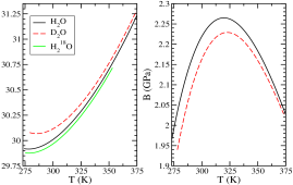
Figure 1: Volume per molecule (left) and bulk modulus (right) as a function of temperature for light and heavy liquid water replotted from Ref. Kell, 1977.

Another open question is the contribution of zero point vibrations to the structure of water and ice Ceriotti et al. (2016). The temperatures at which anomalies occur are different for normal and heavy ice: the temperature of specific heat minimum is $310$K ($330$K) Smirnova et al. (2006), the temperature of maximum density is $277$K ($284$K) Franks (2000); Kell (1967), the temperature of isothermal compressibility minimum is $319.5$K ($322$K) for H₂O (D₂O) Kell (1967). Nuclear quantum effects are also observed in the lattice constants of light and heavy hexagonal ice Ih, as an anomalous isotope effect Röttger et al. (1994), where the larger volume corresponds to the heavier isotope; in contrast to the normal isotope effect, where the lighter isotope induces a larger lattice expansionAllen (1994). Furthermore, this anomalous isotope effect increases up to the melting temperature, and persists to the boiling temperature of liquid water, as measured in temperature dependence of density and compressibility of light and heavy liquid water Kell (1967, 1977); as shown in Fig. 1, which is replotted using Ref. Kell, 1977 eq. (34, 38, 41) for volumes and eq. (35, 39) for compressibility $\kappa$ and bulk modulus $B$, using the relation $B=1/\kappa$.

The primary nuclear quantum effect is revealed in the covalent bond length: $r_{\rm OH}$ is longer than $r_{\rm OD}$. The secondary nuclear quantum effect, also called the Ubbelöhde effect, is revealed in the Hydrogen bond (Hbond) length $r_{\rm OO}$, the Hbond donor-acceptor (oxygen-oxygen) distance. Due to the competing quantum effects Habershon et al. (2009); McKenzie et al. (2014); Li et al. (2011); Zeidler et al. (2011); Markland and Berne (2012); Romanelli et al. (2013); Ceriotti et al. (2016), the change in Hbond length depends on the strength of the Hbond: In a material with a strong Hbond, a librational mode (an out-of-plane zero-point motion of the H atom) increases the Hbond length, while a stretching mode decreases the Hbond length (also called positive Ubbelöhde effect). In a material with a weak Hbond, the opposite effect occurs (negative Ubbelöhde effect) . The Hbond length of ice lies at the crossover between the positive and negative Ubbelöhde effect. To understand the anomalous isotope effect in ice, we developed a method based on ab initio density functional theory (DFT) within quasi-harmonic approximation for the volume dependence of the phonon energy. Using this method, we showed that the anomalous isotope effect is due to the anticorrelations between the Hbond and OH covalent bond in hexagonal ice Pamuk et al. (2012), reflected in the Grüneisen parameters with opposite signs for librational modes and stretching modes. With this method, we also showed that the nuclear quantum effects are the source of the temperature difference between heavy and normal ice at the proton order-to-disorder phase transition of hexagonal ices Pamuk et al. (2015).

In the first section of this paper, we extend our previous studies Pamuk et al. (2012, 2015) to the bulk modulus of hexagonal ices, to understand the links between the isotope effect and the compressibility. We analyze the anisotropy in the bulk modulus, and the nuclear quantum effects on the isotropic bulk modulus of hexagonal ice, to show that the anomaly persists in the bulk modulus calculations.

The second section analyzes the anomalous isotope effect of volume and bulk modulus (i.e. compressibility) of different phases of ice, to gain insight into the isotope effect in liquid water. Recent studies show that the quantum effects on the volume are not always anomalous for all phases of ice. DFT calculations predict a normal isotope effect on the volume of ice VIII Koichiro Umemoto and Baroni (2010); Murray and Galli (2012); Umemoto et al. (2015); Umemoto and Wentzcovitch (2017), which is confirmed by experiments Umemoto et al. (2015). In addition, there has not been a study of isotope effects in different phases of ice that lie in between ice XI and ice VIII. Therefore, we analyze different ice-like structures between these two extremes, with different levels of Hbond, OH covalent bond, and van der Waals (vdW) bond strengths, and interstitial sites. In addition to the polymorphs: ice XI, ice Ih, ice II, ice IX, ice XV, and ice VIII, we study clathrate hydrates, where an anomalous isotope effect has been observed experimentally Klapproth et al. (2003), as well as high density liquid-like (HDL-like) and low density liquid-like (LDL-like) amorphous ice structures, which resemble liquid water due to the structural disorder in these glassy systems. With this analysis, we conclude how nuclear quantum effects change with the structure, and make links between the anomalous isotope effect and the compressibility minimum of liquid water.

II Methodology

II.1 Ice Structures

Fig. 2 shows the ice polymorphs studied in this work. Details of each structure is as follows:

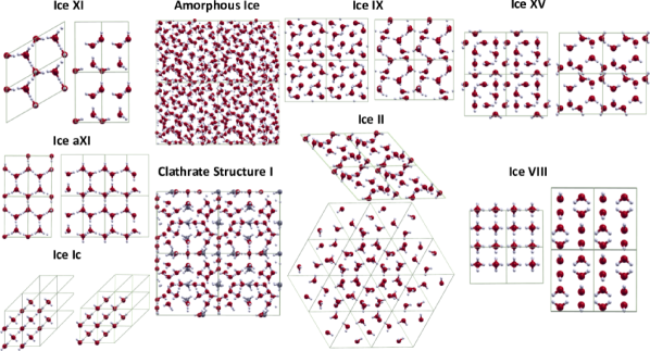
Figure 2: Ice polymorphs studied in this work. Each structure is shown in a $2\times 2\times 2$ super cell, and rotated to better show the periodicity of the unit cell.

II.1.1 Hexagonal ice

The most common phase is hexagonal ice Ih, in which oxygen atoms occupy the hexagonal wurtzite structure, while the hydrogen atoms are disordered. The two covalently-bonded protons have six possible orientations, but are constrained by Bernal-Fowler “ice rules” to have one proton per tetrahedral O-O bond. If ice is catalyzed by KOH^- at 72 K, it goes through a phase transition where the protons order Tajima et al. (1982). Therefore, we consider two possible proton-ordered phases as well as the proton-disordered phase:

(i) Ice XI. This system has 4 molecules in the unit cell. Oxygen atoms are constrained to the hexagonal lattice, and hydrogen atoms have ferroelectric order with a net dipole moment along the c-axis.

ii) Ice aXI. This system has 8 molecules in the unit cell. The oxygen atoms are ordered as in ice XI, but the hydrogen atoms have antiferroelectric order with no net dipole moment.

(ii) Ice Ih. Our model for the H-disordered ice Ih structure has 96 molecules in a $3a\times 2\sqrt{3}a\times 2c$ cell. This system has proton disorder, with no net dipole moment. Both systems have low density liquid like structures.

We have shown before that the order-to-disorder phase transition occurs from the ferroelectric-proton-ordered ice XI, but for completeness, we also present the antiferroelectric-proton-ordered ice aXI Pamuk et al. (2015).

II.1.2 Cubic ice Ic

Cubic ice Ic is metastable with oxygen atoms are arranged in the cubic diamond structure. We only study a proton-ordered structure with 2 molecules in the unit cell.

Ice Ic is formed when the temperature of amorphous ice is increased above $\sim$ 130 K Blackman and Lisgarten (1958). Alternatively, supercooled water crystallizes to ice Ic upon cooling Svishchev and Kusalik (1994). Ice Ic also forms when high pressure phases from ice II to ice IX are recovered in liquid nitrogen and heated Bertie et al. (1963); Bertie and Whalley (1964). Therefore, there is no sharp phase transition between ice Ic and ice Ih. The relationship between the hexagonal ice and the cubic ice is defined by different stacking orders: ice Ih is AB stacked, while ice Ic is ABC stacked. There are also studies on the formation of ice with a mixture of ice Ih and ice Ic, with stacking disorder. We are interested in understanding the isotope effect with changing density. Therefore the stacking disorder between ice Ic and ice Ih is beyond the scope of this work Amaya et al. (2017).

II.1.3 Clathrate hydrate structure I

The clathrate hydrate structure I has two 5¹² cages and six 5¹²6² cages for a total of 46 H₂O molecules per unit cell Román-Pérez et al. (2010). The original structure has a host of 8 CH₄ molecules, but for the purposes of this study, we will focus on the empty clathrate hydrate structure I, which will be denoted as clathrate sI.

II.1.4 Amorphous ices

To approximate amorphous ices, we have taken inherent structures from different ab initio molecular dynamics (AIMD) simulations:

i) One configuration from low density liquid like (LDL-like) structure, taken from AIMD simulations of 128 water molecules with simulation density $\rho=1$g/cm³ with the PBE functional Corsetti et al. (2013).

ii) Two configurations from high density liquid like (HDL-like) structure, taken from AIMD simulations of 64 water molecules with simulation density $\rho=1$g/cm³ with the vdW-DF^PBE functional Wang et al. (2011).

iii) One configuration from high density liquid like (HDL-like) structure, taken from AIMD simulations of 128 water molecules with simulation density $\rho=1.2$g/cm³ with the vdW-DF^PBE functional Corsetti et al. (2013).

These configurations have both proton and oxygen disorder, different from crystalline structures, resembling the structure of liquid water.

II.1.5 Ice IX

Neutron diffraction experiments show that the unit cell of ice IX is tetragonal, with proton ordering J.D et al. (1993); Kuhs et al. (1998), and with 12 molecules in the unit cell. Ice IX forms by a phase transition from metastable proton-disordered ice III. The proton ordering of ice III occurs when high permittivity due to the proton disorder falls gradually at around 173 K Whalley et al. (1968).

II.1.6 Ice II

The structure of ice II is determined both from X-ray Kamb (1964) and neutron diffraction measurements Kamb et al. (1971) to be rhombohedral with $\alpha=113.1^{\circ}$ and with 12 molecules in the unit cell. The experimental angle is kept constant in all calculations. This structure is completely proton ordered. A proton-disordered polymorph of ice II does not exist in the ice phase diagram. Ice II forms when pressure is applied on hexagonal ice Ih at temperatures between 193 K and 231 K, or when pressure is released from ice V at 243 K Whitworth and Petrenko (1999). When ice II is heated, a phase transition to ice III occurs. However, cooling of ice III does not transform it back to ice II. Instead, ice III stays metastable until it transforms into ice IX Whitworth and Petrenko (1999).

II.1.7 Ice XV

The structure of ice XV is determined to be pseudo-orthorhombic from powder neutron diffraction experiments Salzmann et al. (2009). For simplicity, we used a pseudo-tetragonal cell such that the lattice parameters are $a=b\neq c$, with the angles $\alpha=90.1^{\circ}$ and $\beta=\gamma=89.9^{\circ}$ fixed to the experimental values, and with 10 molecules in the unit cell. Ice XV is the antiferroelectric-proton-ordered polymorph of proton-disordered ice VI. Ice XV is stable at temperatures below $\sim 130$ K and pressures between 0.8 to 1.5 GPa Salzmann et al. (2009).

II.1.8 Ice VIII

Ice VIII is determined to be tetragonal from neutron diffraction experiments James D. Jorgensen and Worlton (1984); W. F. Kuhs and Bliss (1984), with 8 molecules in the unit cell, and with two interpenetrated networks, in which molecules of one network occupy the interstitial sites of the other network, each with underlying structure of ice Ic. Within each network, the aforementioned ice rules are satisfied, but there is no Hbond connection between the two networks. The bonding between these unconnected networks is dominated by the van der Waals interaction. Each interpenetrating network have ferroelectric order along the $\hat{z}$-axis with opposite signs, resulting in a net antiferroelectric structure W. F. Kuhs and Bliss (1984); Nelmes et al. (1993); Besson et al. (1994a); Nelmes et al. (1998). Therefore, the inclusion of vdW forces into the calculations become even more important for this case. Previous calculations of the Hbonded O-O networks and non-bonded O$\cdots$O networks do not include vdW effects Umemoto and Wentzcovitch (2004, 2005); Umemoto et al. (2015); Umemoto and Wentzcovitch (2017). The inelastic neutron scattering spectrum of ice VIII shows a weak coupling between the intramolecular and intermolecular modes J-C. Li and Eccleston (1999), which indeed point to a normal isotope effect in this system. Ice VIII and its proton-disordered form ice VII are the most dense ice phases, located at the high pressure region of the ice phase diagram.

II.2 Theory

II.2.1 Free Energy within Quasiharmonic Approximation

To include the nuclear quantum effects, the Helmholtz free energy $F(V,T)$  Ziman (1979) is calculated as a function of volume and temperature in the volume-dependent quasiharmonic approximation (QHA): Pamuk et al. (2012); Ramírez et al. (2012)

$$F(V,T) = E_{0}(V)+$$ (1)

$$\sum_{k}\left[\frac{\hbar\omega_{k}(V)}{2}+k_{B}T\ln\left(1-e^{-\hbar\omega_{k}(V)/k_{B}T}\right)\right].$$

Here $E_{0}(V)$ is the energy for classical (or frozen) nuclei, at the relaxed atomic coordinates of each volume. The volume $V(T)$ and bulk modulus are calculated from the minimum and the curvature of $F(V)$ at each $T$. The phonon frequencies, $\omega_{k}$ are calculated with $k$ running over both the branches and the phonon wave vectors within the Brillouin zone. The volume shift of $\omega_{k}$ is found for each $T$, as parameterized by the Grüneisen parameter:

$$\gamma_{k}=-\frac{\partial({\rm ln}\omega_{k})}{\partial({\rm ln}V)}=-\frac{V}{\omega_{k}}\frac{\partial\omega_{k}}{\partial V}.$$ (2)

In linear approximation this is

$$\omega_{k}(V) = \omega(V_{0})\left(\frac{V}{V_{0}}\right)^{-\gamma_{k}}$$ (3)

$$\approx \omega(V_{0})\left(1-\gamma_{k}\frac{V-V_{0}}{V_{0}}\right).$$ (4)

We have shown previously Pamuk et al. (2012); Ramírez et al. (2012), the QHA as linearized in eq. (4) is an excellent approximation to the full QHA. Other studies also confirm that the QHA is an appropriate method to analyze the isotope effect on the volume and volume derivatives of the energy, such as the bulk modulus Murray and Galli (2012); Koichiro Umemoto and Baroni (2010); Umemoto et al. (2015); Umemoto and Wentzcovitch (2017); Salim et al. (2016).

II.2.2 Bulk Modulus and Pressure

For the bulk modulus calculations, we change the lattice parameters by $0.15\%$ and make a third order polynomial fit to the free energy as a function of volume, $F(V)$ at a given temperature. The curvature of this fit gives the bulk modulus,

$$B=V_{\rm min}\left.\frac{\partial^{2}F}{\partial V^{2}}\right|_{V=V_{\rm min}},$$ (5)

where $V_{\rm min}$ is the minimum of the $F(V)$ curve Allen (2015). For the classical (frozen lattice) bulk modulus $B_{0}$, we use the Kohn-Sham energy $E_{0}$ instead.

The pressure of the system as a function of volume at a given $T$ is calculated from the free energy

$$P(V)=-\frac{\partial F}{\partial V}.$$ (6)

II.3 Computational Methods

We use siesta code with norm-conserving pseudopotentials, and numerical atomic basis sets for the valence electrons, for DFT calculationsOrdejón et al. (1996); Soler et al. (2002). We use two different density functionals: PBE within generalized gradient approximation (GGA) to the exchange and correlation, and vdW-DF^PBE with inclusion of long range van der Waals interactions Perdew et al. (1996); Dion et al. (2004); Román-Pérez and Soler (2009); as well as the TTM3F force-field method Fanourgakis and Xantheas (2008), for the bulk modulus calculations of hexagonal ices. For the rest of the ice-like structures, we present only the results with the vdW-DF^PBE functional, since the inclusion of the vdW forces has been shown to be crucial in the analysis of ice polymorphs Santra et al. (2013); Pamuk et al. (2015). Comparison of the results with the PBE functional can be found in Ref. Pamuk (2014).

For hexagonal ices, the same procedure is followed as Ref. Pamuk et al. (2012, 2015) All initial structural relaxations are done by the t$\zeta$+p atomic orbital basis set for ice Ic, clathrate sI, and amorphous ices, and the d$\zeta$+dp atomic orbital basis set developed in Ref. Corsetti et al. (2013) for ice IX, ice II, ice XV, and ice VIII. We use a real-space mesh cutoff of 500-600 Ry for the real space integrals, an electron momentum Monkhorst-Pack grid of $6\times 6\times 6$ for unit cell calculations, a force tolerance of 0.005-0.001 eV/Å , and a density matrix tolerance of $10^{-4}$-$10^{-5}$ electrons. Further details of these parameters for each structure can also be found in Ref. Pamuk (2014). For the volume dependence of the Kohn-Sham energy, the electronic energy of these relaxed configurations are recalculated using the q$\zeta$+dp atomic orbital basis sets. The curve for Kohn-Sham energy as a function of volume $E_{0}(V)$ is obtained and the classical (frozen) volume $V_{0}$ is calculated from the minimum of a third order polynomial fit.

For nuclear quantum effects, the vibrational modes are calculated using the frozen phonon approximation. All force constants calculations are performed with the same basis sets with which the initial relaxations are performed. We used an atomic displacement $\Delta x$=0.06-0.08 Å  for the frozen phonon calculation. The phonon frequencies, $\omega_{k}(V_{0})$ and Grüneisen parameters $\gamma_{k}(V_{0})$ are obtained by diagonalizing the dynamical matrix, computed by finite differences from the atomic forces, at volumes slightly below and above $V_{0}$. For crystalline ices, a $3\times 3\times 3$ super cell is used. The Grüneisen parameters are calculated for 3 volumes, and the phonon modes are calculated by dividing Brillouin zone to a grid of $9\times 9\times 9$, with equal weights.

III Results

III.1 Bulk Modulus of Hexagonal Ices

III.1.1 Anisotropy in Classical Bulk Modulus

We first determine optimal lattice parameters of hexagonal ices. Lattice parameters are kept constant at each ionic relaxation, and varied systematically to cover $E_{0}(a,c)$ surface. The optimal lattice parameters are selected both considering the minimum of $E_{0}(a,c)$ surface, and $E_{0}(V)$ curve, at $P=0$.

Table 1: $a$ and $c$ lattice parameters, their ratio ($c/a$), and the corresponding volume per molecule, Volume/H₂O$=a^{2}c\sqrt{3}/2/N_{{\rm H_{2}O}}$, for the force field model (FF) or exchange and correlation functional (XC). All lengths are in Å  and volumes in ų.

FF/XC	Ice	$a$	$c$	$c/a$	Volume/H2O
TTM3-F	Ih	4.54	7.41	1.632	33.07
TTM3-F	aXI	4.55	7.41	1.629	33.21
TTM3-F	XI	4.54	7.43	1.637	33.16
PBE	Ih	4.42	7.21	1.631	30.49
PBE	aXI	4.42	7.21	1.631	30.49
PBE	XI	4.42	7.21	1.631	30.49
vdW-DFPBE	Ih	4.45	7.27	1.634	31.17
vdW-DFPBE	aXI	4.46	7.25	1.624	31.18
vdW-DFPBE	XI	4.45	7.25	1.629	31.08
Expt. Röttger et al. (1994) 10K $\rm{H_{2}O}$	Ih	4.497	7.321	1.628	32.05
Expt. Röttger et al. (1994) 10K $\rm{D_{2}O}$	Ih	4.498	7.324	1.628	32.08
Expt. Line and Whitworth (1996) 5K $\rm{D_{2}O}$	Ih	4.497	7.324	1.629	32.07
Expt. Line and Whitworth (1996) 5K $\rm{D_{2}O}$	XI	4.501	7.292	1.620	31.98

Table. 1 gives calculated lattice parameters of all three hexagonal ice structures, as well as the experimental results obtained for both heavy and light ice by synchrotron radiation Röttger et al. (1994). We also present experimental lattice parameters from Ref. Line and Whitworth, 1996 as they study neutron diffraction of both ice XI and ice Ih. They compare the orthorhombic structure of ice XI with the hexagonal structure of ice Ih. Since we keep hexagonal symmetry in our ice XI calculations, we compare to experimental lattice parameters $\sqrt{(ab/\sqrt{3})}$ of ice XI Line and Whitworth (1996). In this case, the experimental lattice parameter $a$ changes very slightly from ordered to disordered phase, whereas the lattice parameter $c$ changes significantly.

The TTM3-F force-field model predicts that ice XI has a larger volume than ice Ih, which is opposite to the experimental results; and ice aXI has the largest volume. The change is caused by the lattice parameter $a$, when ordering is from ice aXI to ice Ih; and by $c$, when ordering is from ice XI to ice Ih. Changes in the $c$ are in opposite directions between the TTM3-F model and the vdW-DF^PBE functional. The PBE functional predicts that both proton-ordered ices (ice XI and aXI) have the same lattice parameter as ice Ih. The vdW-DF^PBE functional predicts that the antiferroelectric-ordered ice aXI has larger volume than both ice Ih and ice XI. The lattice parameter $a$ ($c$) of ice aXI is larger (smaller) than that of ice Ih, while the difference in the volume of ice aXI and ice XI is only due to the change in the lattice parameter $a$. Ferroelectric-ordered ice XI has a smaller volume than ice Ih. This change in volume is due to the change in the lattice parameter $c$, in good agreement with experiments, again showing the importance of van-der Waals forces in calculations. vdW-DF^PBE gives lattice changes similar to experiments between the ferroelectric-ordered ice XI and proton disordered ice Ih. This agrees with our previous prediction that the proton order-to-disorder phase transition is from the ferroelectric-ordered ice XI to ice Ih Pamuk et al. (2015).

Considering the hexagonal structure of ice, with different lattice parameters along different directions as explained above, the bulk modulus of ice is expected to be different with respect to the compressions along the $x$-$y$ plane and $z$-axis. Components of the strain tensor are different for displacements along different directions. We consider three contributions to strain tensor:

i) $(C_{11}+C_{12})/2$, keeping lattice parameter $c$ constant, while changing $a$ by $0.15\%$. This shows how the bulk modulus is affected changes along the x-y plane.

ii) $C_{33}$, keeping lattice parameter $a$ constant, while changing the lattice parameter $c$ by $0.15\%$. Similarly, this shows how the bulk modulus is affected changes along the z-axis.

iii) $C_{13}$, using the relation between the isotropic bulk modulus and other components:

$$B=\frac{C_{33}(C_{11}+C_{12})-2C_{13}^{2}}{C_{11}+C_{12}+2C_{33}-4C_{13}}$$ (7)

The relations between strain tensor and bulk modulus, and the derivation of eq. (7) are explained in detail in the Supporting Information (SI). The strain tensor components and the bulk modulus results are summarized in Table 2. In addition, we check eq. (7) against the experimental data of Ref Gagnon et al., 1988 in the last two rows of Table 2. Using experimental values of B₀, ($C_{11}+C_{12}$)/2, and $C_{33}$, we have calculated $C_{13}$. The calculated compared reasonably with experiment, considering the spread both in the experimental and theoretical results.

Table 2: The classical bulk modulus and the related components of the strain tensor in units of GPa. Experimental results are extrapolated to T=0K from eq. (4) of Ref Gagnon et al., 1988. ^e is the experimental result from the reference, and ^c is the calculated result using eq. (7).

FF/XC	Ice	B0	($C_{11}+C_{12}$)/2	$C_{33}$	$C_{13}$
TTM3-F	Ih	13.7	15.0	20.3	10.8
TTM3-F	aXI	14.1	14.8	20.4	12.2
TTM3-F	XI	14.2	14.4	20.8	13.3
PBE	Ih	14.2	17.4	27.1	7.9
PBE	aXI	14.3	17.5	26.9	8.0
PBE	XI	14.3	17.4	26.3	8.2
vdW-DFPBE	Ih	13.5	15.7	21.9	9.3
vdW-DFPBE	aXI	14.1	16.2	20.8	10.4
vdW-DFPBE	XI	14.3	16.1	22.1	10.6
Expt Gagnon et al. (1988)	Ih	8.48	10.31	14.76	5.63e
Expt Gagnon et al. (1988)	Ih	8.48	10.31	14.76	5.09c

The experimental results spread over a range between 7-12 GPa, for the bulk modulus of proton disordered ice Ih. Few authors comment on the anisotropic components Feistel and Wagner (2006). The experimental results Gagnon et al. (1988) in Table 2 lie on the lower end of this spread when isotropic bulk moduli are compared Gagnon et al. (1988); Feistel and Wagner (2006). However, they still give a qualitative intuition about the order of magnitude of different components of the strain tensor. Comparing our calculations of anisotropic bulk modulus along different directions, shows that bulk modulus along the xy-plane, $(C_{11}+C_{12})/2$, is smaller than that along the z-axis, ($C_{33}$). Hexagonal ice is softer along the x-y plane than along the z-axis.

Without a bulk modulus experiment on proton-ordered ice XI it is difficult to comment on structural differences between ice XI and ice Ih. The TTM3-F force field model gives no net trend between different components of the strain tensor, and an inconsistency between lattice parameter and bulk modulus. Focusing on the structural differences between the ferroelectric-ordered ice XI and proton disordered ice Ih, with the semilocal PBE functional, all components of the strain tensor are similar. When non-local vdW forces are included using the vdW-DF^PBE functional, both the isotropic and anisotropic moduli of ice XI are clearly larger than those of ice Ih. This predicts that disordered ice Ih is softer than ordered ice XI. The vdW-DF^PBE functional gives more reasonable bulk modulus results that are consistent with the trend in the volume and lattice parameters.

III.1.2 Nuclear Quantum Effects on Bulk Modulus

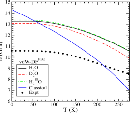
Figure 3: Bulk modulus as a function of temperature calculated with the QHA using the vdW-DF^PBE functional for proton-ordered ice XI. The experimental results are taken from Ref. Feistel and Wagner, 2006.

Table 3: The bulk modulus of hexagonal ices including the quantum zero point effects in units of GPa, as well as the isotope effect on the bulk modulus IS(A-B)=$\frac{B({\rm A})}{B({\rm B})}-1$ between the isotopes A and B.

FF/XC	Ice	B0	H2O	D2O	H${}_{2}\text{}^{18}$O	IS(H-D)	IS(16O-18O)
TTM3-F	Ih	13.74	12.81	12.85	12.86	$-0.31\%$	$-0.39\%$
TTM3-F	aXI	14.13	13.03	13.08	13.09	$-0.38\%$	$-0.46\%$
TTM3-F	XI	14.24	13.04	13.09	13.10	$-0.38\%$	$-0.46\%$
PBE	Ih	14.24	14.18	13.44	14.33	$+5.22\%$	$-1.06\%$
PBE	aXI	14.31	13.79	13.15	13.95	$+4.63\%$	$-1.17\%$
PBE	XI	14.27	13.70	13.18	13.84	$+3.80\%$	$-1.02\%$
vdW-DFPBE	Ih	13.52	13.45	13.43	13.46	$+0.15\%$	$-0.07\%$
vdW-DFPBE	aXI	14.05	13.36	13.23	13.43	$+1.00\%$	$-0.53\%$
vdW-DFPBE	XI	14.32	13.26	13.06	13.37	$+1.51\%$	$-2.37\%$
Expt. Hamada (2010); Gammon et al. (1983)	Ih		12.1
Expt. Gagnon et al. (1988)	Ih		8.48
Expt. Herrero and Ramírez (2011); Feistel and Wagner (2006)	Ih		10.9

We also estimate the contributions from quantum zero point effects by calculating the curvature of free energy calculations in eq. (1). We computed the phonon density of states and corresponding Grüneisen parameters, $\gamma_{k}$, of all structures, as described in eq. (2). Accurate estimation of Grüneisen parameter is crucial, because the average value $\langle\omega_{k}\gamma_{k}\rangle$ determines whether a system has a normal or anomalous isotope effect Pamuk et al. (2012). In the normal isotope effect, the bulk modulus of the heavier isotope is larger, whereas in the anomalous isotope effect, the bulk modulus of the lighter isotope is larger. Negative $\gamma_{k}$’s imply a softening of the modes with decreasing volume, favoring larger bulk modulus for the lighter isotope.

Within each structure, considering how frequencies and Grüneisen parameters are distributed, we separate phonon modes into 6 groups. Fig. 4 and 5 show phonon density of states and Grüneisen parameters of each mode. The average phonon frequencies and the corresponding average $\gamma_{k}$ for each group can be found in the SI of Ref. Pamuk et al. (2015). First, there is a band with small frequencies ($\omega\sim 74$ cm^-1), associated with the stretching modes of the Hbond, that has negative $\gamma_{k}$, responsible for the negative thermal expansion of hexagonal ice. Röttger et al. (1994) The translational modes ($\omega\sim 271$ cm^-1) are mostly dominated by oxygen atoms, while the libration modes ($\omega\sim 847$ cm^-1) are dominated by the hydrogen atoms. These two modes both contribute to the strength of Hbonding network, and they have positive $\gamma_{k}$, favoring the normal isotope effect. The bending modes ($\omega\sim 1646$ cm^-1) are very harmonic and have very small $\gamma_{k}$, and a small effect on the isotope effect. These modes do not contribute to the interplay between covalent bond and Hbond network. The highest frequencies correspond to the anti-symmetric ($\omega\sim 3314$ cm^-1 for H₂O) and symmetric ($\omega\sim 3115$ cm^-1 for H₂O) stretching modes of the OH covalent bond, with weight mostly on the hydrogen atoms. The stretching modes have negative $\gamma_{k}$’s, favoring anomalous isotope effect. There is an anti-correlation between the translational and librational modes which determine the strength of the Hbond and the stretching modes which determine the strength of the OH covalent bond. The anomalous isotope effect is a result of a fine balance between cancellations of contributions from each band Pamuk et al. (2012); Ganeshan et al. (2013).

Results for the bulk modulus at $T=0$ K are in Table 3. The temperature dependence of the bulk modulus is given in Fig. 3 for ferroelectric-proton-ordered ice XI, calculated with the vdW-DF^PBE functional.

The TTM3-F force field model does not correctly predict anomalous isotope effect at low temperatures. Temperature dependence of bulk modulus for ice XI and ice Ih with TTM3-F model are in SI. With this model, there is a crossing from normal to anomalous isotope effect at $\sim 270$ K, close to the melting temperature, where the low frequency modes with $\gamma_{k}>0$ become classical, and high frequency modes with $\gamma_{k}<0$ dominate the quantum effects Ganeshan et al. (2013).

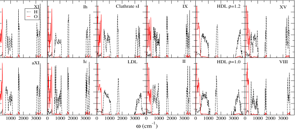
Figure 4: Phonon density of states for H₂O, projected onto H and O atoms, obtained with the vdW-DF^PBE functional.

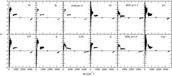
Figure 5: Average Grüneisen parameter of each phonon mode, obtained with the vdW-DF^PBE functional.

DFT calculations reproduce the anomalous effect on the isotopes of hydrogen atoms, i.e the bulk modulus of H₂O is larger than the bulk modulus of D₂O. Similarly to the volume isotope effect Pamuk et al. (2012), the bulk moduli of oxygen isotopes are predicted to have a normal isotope effect, i.e the bulk modulus of H₂O is smaller than the bulk modulus of H${}_{2}\text{}^{18}$O. This behavior is reproduced qualitatively for both DFT functionals. Comparing with previous DFT plane wave studies Murray and Galli (2012), our PBE calculations perform quite similarly. However, plane wave calculations that include van der Waals forces with the vdW-DF2 functional Lee et al. (2010) do not give the anomalous isotope shift. Therefore, the vdW-DF^PBE functional is a better candidate for this type of analysis. There is still room for improvement of van der Waals forces representation with the density functionals Santra et al. (2013).

As the temperature increases, the bulk modulus of all ices decrease. The convergence to the classical bulk modulus occurs at the temperatures much higher than the melting temperature of ice. This is an indication that the nuclear quantum effects are still important in the liquid water and must be considered for the correct structural analysis.

III.2 Nuclear Quantum Effects in Other Ice Polymorphs

Experiment shows that the anomalous volume isotope effect of the replacement of H with D, also persists in liquid water, Kell (1967, 1977) although the structure of the liquid is very different from hexagonal ice. Therefore, we turn our focus to other crystalline ice phases and ice-like structures with varying densities in order to understand the isotope effect on the volumes and compressibility.

As before, we start with an analysis of the density of states and the Grüneisen parameters, $\gamma_{k}$, of all structures, as given in Fig. 4 and 5. The trends in frequencies and corresponding Grüneisen parameters seen in hexagonal ices persist in ice Ic and clathrate sI, and also in LDL-like amorphous ice. However, as the density increases, some of the low frequency bands start mixing and are harder to differentiate into groups. The first difference appears in the low frequency group with negative $\gamma_{k}$, associated with the stretching of the Hbond and the negative Grüneisen parameters and responsible for the negative thermal expansion of hexagonal ice. Röttger et al. (1994) This band has negative $\gamma_{k}$ for ice Ic and clathrate sI; its Grüneisen parameters start to become positive in amorphous ices, and high density crystalline ices, ice IX, ice II, ice XV, and ice VIII. Consequently, a negative thermal expansion is observed in ice Ic at $\sim 60$ K and in empty clathrate sI at $\sim 70$ K, and this behavior is not observed in rest of the crystalline phases. However, this band is not dominant in the determination of the isotope effect in general. The translational modes and the libration modes that are linked to the Hbonding network both mostly have positive $\gamma_{k}$, favoring the normal isotope effect. For all structures, the bending modes are very harmonic and they have very small $\gamma_{k}$, hence these modes are not effective enough on the isotope effect. The highest frequencies, which correspond to the anti-symmetric and symmetric stretching modes of the OH covalent bond with a weight mostly on the hydrogen atoms, have negative $\gamma_{k}$, favoring the anomalous isotope effect. For the crystalline phases and empty clathrate sI, it is possible to distinguish between the symmetric and anti-symmetric stretching modes, while for amorphous ices these modes are mixed, similar to the phonon density of states of liquid water. The anti-symmetric stretching modes have in general less negative $\gamma_{k}$ as compared to the symmetric stretching modes. In addition, these modes become less and less negative as the density of the ice phase increases going from ice XI towards ice VIII. Again, the fine balance between the translational and librational modes, which are linked to the strength of the Hbond, and the stretching modes, which are linked to the strength of the OH covalent bond, determine whether the system has a normal or anomalous isotope effect.

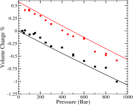
Figure 6: Volume change $V(P)/V_{\rm{H_{2}O}}(0)-1$, relative to H₂O at $P=0$ bar for empty clathrate structure I. The lines are the calculations and the dots are the experimental values taken from Ref. Klapproth et al. (2003).

The isotope effect on the volume of the clathrate sI is known to be anomalous from the experiments Klapproth et al. (2003), therefore we first focus on this structure to compare our calculations. We calculate the free energy profiles of corresponding experimental temperatures, T = 271 K for H₂O and T = 273 K for D₂O and obtain the relation between the pressure and the volume, as explained in eq. (6). To compare the isotope shift in clathrate sI, the experimental H₂O volume at the lowest experimental pressure, and the calculated H₂O volume at zero pressure are both set to zero; and Fig. 6 shows the relative change in the volume from H₂O to D₂O. These results show that the anomalous isotope effect in clathrate sI, as well as the amount of the shift in the volume, is well captured with the vdW-DF^PBE functional. Even though there is a difference in the slopes of the experimental and the theoretical values, which is reflected in the bulk modulus results, the net isotope shift in the volume is well represented within the QHA. The isotope shift is similar for the filled structures, and is presented in the SI. Similarly to the isotope effect in volume, the isotope effect in the bulk modulus is also anomalous.

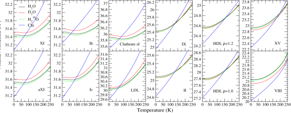
Figure 7: Volume per molecule as a function of temperature calculated with the QHA using the vdW-DF^PBE functional.

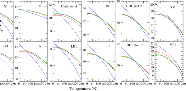
Figure 8: Bulk modulus as a function of temperature calculated with the QHA using the vdW-DF^PBE functional.

Next, we present the volume and bulk modulus as a function of temperature for all structures in Fig. 7 and Fig. 8 respectively. The low density crystalline ices: hexagonal ices and cubic ice have a similar structure with a volume per molecule of $V\sim 31.5$ Å  at $T=0$ K, and a bulk modulus of $B\sim 13$ GPa. The empty clathrate sI has slightly larger volume per molecule $V\sim 36$ Å, and smaller bulk modulus $B\sim 10.5$ GPa, and these results are in general good agreement with the experiments Klapproth et al. (2003). The LDL-like amorphous ice has smaller volume per molecule $V\sim 30$ Å  and bulk modulus $B\sim 8$ GPa, which is close to that of liquid water. The crystalline ices that are in the middle of the pressure range of the phase diagram: ice IX and ice II both have a volume per molecule of $V\sim 25$ Å, and this is in good agreement with the experiments J.D et al. (1993); Kamb (1964). At $T=225$ K, the volume for ice II is in good comparison with the experimental value of $V=25.6$ Å, while the bulk modulus $B\sim 15$ GPa is larger than the experimental value of $B=12.13$ GPa Fortes et al. (2005). There is no data, to our knowledge, on the bulk modulus of ice IX, therefore we comment on its proton-disordered polymorph ice III that has an experimental bulk modulus very similar to the bulk modulus of ice Ih $B\sim 9.6$ GPa Gagnon et al. (1990), which agrees with our results that the bulk modulus stays $B\sim 13$ GPa slightly decreasing from ice XI to ice IX. The volume per molecule decreases as we get to ice XV; the experimental volume per molecule is $V=22.5$ ÅSalzmann et al. (2009), and is slightly smaller than our calculated result of $V\sim 23$ Å. Again due to the lack of bulk modulus data of ice XV, we compare to its proton-disordered polymorph ice VI, and the bulk modulus increases significantly to $B=18.5$ GPa Gagnon et al. (1988), which agrees with the trend of the increase in our calculated bulk modulus results. This trend of decrease in the volume and increase in the bulk modulus also occurs going from LDL-like amorphous ices to HDL-like amorphous ices. Ice VIII has the smallest volume per molecule among all the structures, and the calculated value $V\sim 21$ Å  slightly overestimates as compared to experiments under pressure W. F. Kuhs and Bliss (1984). Consequently, the calculated bulk modulus $B\sim 16$ GPa is underestimated as compared to the recently reported experimental value of $B=18.7$ GPa Klotz et al. (2017), and also as compared to its proton-disordered polymorph ice VII $B=20.4$ GPa Ludl et al. (2017); Besson et al. (1994b). We continue our analysis with the isotope effect, and we present, for completeness, the isotope effect of the oxygen atoms both on the volume and bulk modulus, which stays as normal isotope effect for all structures, but in the following discussion, we focus on the isotope effect of the hydrogen atoms.

The isotope effect at $T=0$ K is anomalous and it stays anomalous up to the melting point for low density structures: hexagonal ices, ice Ic, clathrate sI and LDL-like ices. As the density of the structure increases, going towards ice IX, ice II, and ice XV, as well as in HDL-like amorphous ices, the isotope effect is normal at low temperatures, with a transition to the anomalous isotope effect at higher temperatures. Although it is not possible to exactly determine the temperature of the crossing from normal isotope effect to anomalous isotope effect, we can observe qualitatively that the higher the density, the higher the crossing temperatures. And finally, the isotope effect is normal up to the melting point for ice VIII, which has the highest density. All the results are given at zero pressure, however some of these structures are stable only under applied pressure. Therefore, we also present the isotope effect in volume of ice VIII under 2.5 GPa as a comparison in the SI, and the conclusions we draw do not change. The trends on the isotope effect on the bulk modulus follow the isotope effect on the volume. The isotope effect on the bulk modulus also starts anomalous at low density ice structures and then presents a crossing from normal to anomalous isotope effect as the density of the structure increases. Finally, at the highest density structure of ice VIII, it stays normal up to the melting point. This is depicted on the phase diagram in Fig. 9 as adapted from Ref. Zhang et al., 2015. Blue shaded area shows the ice phases that have the anomalous effect, the crossing region in white shows the ice phases that are at the crossing of the normal and anomalous effects, and the red region shows the ice phases that have the normal isotope effect.

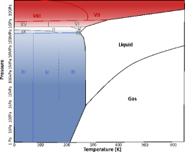
Figure 9: Isotope effect on the phase diagram of water (adapted from Ref. Zhang et al., 2015). Blue, low pressure region: ice phases with the anomalous isotope effect. White, crossing region: ice phases at the crossing of normal to anomalous isotope effect. Red, high pressure region: ice phases with the normal isotope effect.

Table 4: Average oxygen-oxygen distance in Å  for Hbonded and vdW bonded configurations and average number of bonds per molecule for different configurations of structures. The quantum H₂O volume in ų and bulk modulus in GPa with their isotope effect from hydrogen to deuterium, IS_V(H-D)=$\frac{V({\rm H})}{V({\rm D})}-1$ and IS_B(H-D)=$\frac{B({\rm H})}{B({\rm D})}-1$ at zero temperature and pressure are also included.

Ice	$<r_{\rm OO}^{\rm{Hbond}}>$	$<N^{\rm{Hbond}}>$	$<r_{\rm OO}^{\rm{vdW}}>$	$<N^{\rm{vdW}}>$	$V_{\rm{H_{2}O}}$	ISV(H-D)	$B_{\rm{H_{2}O}}$	ISB(H-D)
XI	2.719	4.000	0.000	0.000	31.41	$-0.32\%$	13.26	$+1.51\%$
Clathrate sI	2.728	4.000	0.000	0.000	35.90	$-0.20\%$	10.56	$+1.71\%$
LDL-like${}^{\rho=1.0}_{T=300}$	2.765	3.953	3.899	0.688	30.07	$-0.18\%$	8.28	$+0.81\%$
Ic	2.719	4.000	0.000	0.000	31.60	$-0.16\%$	13.24	$+1.02\%$
HDL-like${}^{\rho=1.2}_{T=300}$	2.815	4.047	3.582	2.109	24.57	$+0.09\%$	16.73	$-0.38\%$
IX	2.737	4.000	3.489	2.000	25.44	$+0.10\%$	13.18	$-0.456\%$
II	2.756	4.000	3.487	2.000	25.10	$+0.12\%$	17.27	$-0.666\%$
HDL-like2${}^{\rho=1.0}_{T=300}$	2.783	4.063	3.748	0.969	27.81	$+0.15\%$	10.80	$-0.59\%$
HDL-like1${}^{\rho=1.0}_{T=300}$	2.790	4.063	3.622	0.969	27.71	$+0.28\%$	9.90	$-1.66\%$
HDL-like${}^{\rho=1.0}_{T=350}$	2.917	3.781	3.834	1.938	27.63	$+0.35\%$	9.69	$-5.21\%$
XV	2.773	4.000	3.354	2.800	22.94	$+0.35\%$	17.12	$-2.40\%$
VIII	2.943	4.000	2.949	4.000	21.09	$+0.90\%$	16.22	$-7.40\%$

These observations let us make one final analysis on these systems. Table 4 shows the average distance between oxygen atoms when they are Hbonded, $<r_{\rm OO}^{\rm{Hbond}}>$, van der Waals bonded $<r_{\rm OO}^{\rm{vdW}}>$, and the average number of each bond in the analyzed configurations. Also included are the isotope effect with respect to H₂O and its quantum volume. The structures are listed from the most anomalous to the least anomalous in the isotope effect on the volume.

For the structures with anomalous effect, the Hbond length is small and is highly populated, while those systems have no (ice XI, clathrate sI, ice Ic) or very few (LDL-like amorphous) vdW bonds. As the density of the structures increases (ice IX, HDL-like amorphous, ice II), Hbond length keeps increasing, but more importantly, these systems have more van der Waals bonds, populating the interstitial sites. Then the effect starts to become normal, but small, and a transition to anomalous isotope effect happens at high temperatures. In the most extreme case of ice VIII, both Hbond length is the largest, vdW bond length is the smallest and the number of vdW bonds is the largest. Then, for all temperatures and pressures, the isotope effect stays normal.

This shows that the density or the $r_{\rm OO}$ distance by itself is not enough to predict the sign of the isotope effect. For example for HDL-like${}^{\rho=1.2}_{T=300}$ structure, in spite of the fact that $r_{\rm OO}$ distance of both bonds are larger than ice IX and ice II, the volume is smaller (density is larger). This is because both bonds are more populated, leading to a conclusion of smaller volume per molecule and a normal isotope effect, after all. Another example is ice VIII where the experimental Hbond distance is $r_{\rm{OO}}^{\rm{Hbond}}=2.979(1)$Å  W. F. Kuhs and Bliss (1984), and for the vdW-DF^PBE functional it is $r_{\rm{OO}}^{\rm{Hbond}}=2.943$Å. Then, each molecule has four vdW bonded (non-bonded) configurations, two of which are closer than the Hbond distance, and two further away. Experimentally, the vdW bonded configuration distance is: $r_{\rm{OO}}^{\rm{vdW1}}=2.743(9)$Å  W. F. Kuhs and Bliss (1984) and for vdW-DF^PBE functional it is $r_{\rm{OO}}^{\rm{vdW1}}=2.822$Å. The second vdW bonded configuration distance for vdW-DF^PBE functional is: $r_{\rm{OO}}^{\rm{vdW2}}=3.075$Å, resulting an average of 4 vdW bond lengths of $r_{\rm{OO}}^{\rm{vdW}}=2.949$Å. Therefore, there is a fine balance between the bond length distances and how many bonds each molecule has. This discussion agrees with recent predictions on the isotope effect in other ice phases Umemoto et al. (2015); Umemoto and Wentzcovitch (2017).

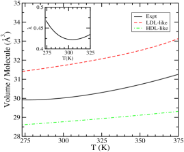
Figure 10: Volume per molecule calculated with the QHA at the liquid water temperatures for the LDL-like amorphous ice and the HDL-like amorphous ice is compared to the experimental values for the liquid. The inset shows what the LDL-like contribution $\lambda$, such that $\lambda V^{\rm LDL-like}+(1-\lambda)V^{\rm HDL-like}=V^{\rm expt.}$

Finally, we can make some links to liquid water, by exploiting the experimental results on the isotope effect on the volume of liquid water Kell (1967, 1977). Considering the difference between the volume per molecule of liquid water with D₂O and H₂O, $V_{\rm D_{2}O}-V_{\rm H_{2}O}$, from Fig. 1, the volume difference decreases with increasing temperature, therefore the isotope effect goes from strongly anomalous towards weakly anomalous, but not crossing up to the boiling temperature. There are two different regions: a region with rapidly decreasing difference $V_{\rm D_{2}O}-V_{\rm H_{2}O}$ going from anomalous towards a normal isotope effect, up to $T\sim 310$ K, and a second region with almost constant, slowly decreasing difference, up to the melting temperature. As the Hbonding network is never completely broken in liquid water, as in ice VIII, the isotope effect stays anomalous throughout all the temperatures. Drawing conclusions from our results, we speculate that the anomalous isotope effect in liquid water goes from strongly anomalous to weakly anomalous as the temperature increases from the melting point to the bulk modulus maximum (compressibility minimum), therefore the LDA-like components of the liquid decrease in this region. Then it starts behaving as a normal liquid after this temperature.

This is also shown in Fig. 10, where the volume per molecule of the liquid water from Ref. Kell, 1977 is compared to one of the configurations with the LDL-like amorphous ice and to one of the configurations with the HDL-like amorphous ice, as calculated with the QHA at high temperatures. Even though the quantitative values are not exact at these temperatures with the QHA, one can estimate the LDL-like and HDL-like contributions to the liquid by approximating the liquid water volume per molecule such that $V^{\rm expt.}=\lambda V^{\rm LDL-like}+(1-\lambda)V^{\rm HDL-like}$. Then it is clear that up to $\sim 305$ K, the LDL-like contributions decrease. Therefore, a force-field model that can reproduce the aforementioned anomalies of water must also reproduce the anomalies in the isotope effect.

IV Conclusion

We study the nuclear quantum effects on the volume and bulk modulus of several ice phases, as well as ice-like structures. We start with a structural analysis of the lattice parameters and the volume of hexagonal ices, including different components of the strain tensor and we show that the classical (frozen) bulk modulus along the x-y plane is smaller than along the z-axis, hence the hexagonal ice is softer along the x-y plane. In addition, we calculate the isotope effect on the total bulk modulus of the hexagonal ices. There is an anomalous isotope effect on the bulk modulus for hydrogen isotopes: the bulk modulus of D₂O is smaller than H₂O, and normal isotope effect on the bulk modulus for oxygen isotopes; similarly to the isotope effect on the volume.

Then we investigate the isotope effect on different polymorphs of ice. First, we obtain an anomalous isotope effect on the volume of the clathrate structure I, in very good agreement with the experiments. Then we calculate that the isotope effect is anomalous in ice Ih, clathrate sI, ice Ic and LDL-like amorphous ices. Moving on to high pressure ice phases, where the interstitial sites start to get filled, in the intermediate ice phases, ice IX, ice II, and ice XV, as well as in the HDL-like amorphous ices, we observe that the difference between the volumes of H and D starts as a small and normal isotope effect and becomes anomalous at higher temperatures with the increasing density. Once we get to the other end of the phase diagram, ice VIII is the most dense ice phase, where the interstitial sites are completely filled, the isotope effect becomes completely normal both at zero pressure and at high pressures.

Finally, we discuss the implications of our results on the isotope effect in liquid water. When the hexagonal ice Ih, which is already a structure with large anomalous isotope effect, melts, the effect in liquid water also starts as large and anomalous. With the increasing temperature, the anomaly of the isotope effect (difference in the volume of the two isotopes) decreases rapidly up to $T\sim 310$ K, which is close to isothermal compressibility minimum temperature, $T\sim 320$ K. Until the compressibility minimum temperature, as the interstitial sites are being filled, the isotope effect goes towards being normal very quickly. This is similar to moving from ice Ih towards ice VIII in the analyzed structures. However, in liquid water, the Hbond network is intact as compared to ice VIII. Therefore, the net effect stays anomalous. Once the compressibility minimum is reached, then the change in the isotope effect is stabilized and it keeps on decreasing at a much slower rate, until it gets to the boiling temperature. With this, we can speculate that the nuclear quantum effects and the anomalous isotope effect are linked to the compressibility minimum of liquid water. This conclusion opens new horizons for the development of semi-empirical water models, showing that a complete theory should be able to explain different anomalies of water, in different regions of the phase diagram.

V Acknowledgments

This work is supported by DOE Grants No. DE-SC0003871 (M.V.F.S.), and No. DE- FG02-08ER46550 (P.B.A.) and the grant FIS2012-37549-C05 from the Spanish Ministry of Economy and Competitiveness. This work used the resources at the Center for Functional Nanomaterials, Brookhaven National Laboratory, which is supported by the U.S. Department of Energy, Office of Basic Energy Sciences, under Contract No. DE-AC02-98CH10886 and No. DE-SC0012704; at the Extreme Science and Engineering Discovery Environment (XSEDE), which is supported by National Science Foundation grant number ACI-1548562; and at the Handy and LI-Red computer clusters at the Stony Brook University Institute for Advanced Computational Science. B.P. acknowledges National Science Foundation [Platform for the Accelerated Realization, Analysis, and Discovery of Interface Materials (PARADIM)] under Cooperative Agreement No. DMR-1539918 for her time at Cornell University.

VI Supporting Information

In the supporting information, we present a detailed derivation of the relations between the strain tensor and the bulk modulus, that is used to calculate the anisotropy in the bulk modulus of the hexagonal ices. We also present the temperature dependence of the bulk modulus of the hexagonal ices as calculated with the TTM3-F force-field model, comparison of the isotope effect of the filled and empty clathrate structures, and the isotope effect on the volume of ice VIII at $P=2.5$ GPa.

VI.1 Strain Tensor and Bulk Modulus Relations

When there is a small uniform deformation on a solid, the axes are distorted in orientation by $\epsilon_{\alpha\beta}$. Kittel (2005) Then the displacement of an atom due to this deformation can be defined as:

$$\mathbf{R}(\mathbf{r}) \equiv (x\epsilon_{xx}+y\epsilon_{yx}+z\epsilon_{zx})\hat{x}+(x\epsilon_{xy}+y\epsilon_{yy}+z\epsilon_{zy})\hat{y}$$ (8)

$$+(x\epsilon_{xz}+y\epsilon_{yz}+z\epsilon_{zz})\hat{z}$$

$$= u(\mathbf{r})\hat{x}+v(\mathbf{r})\hat{y}+w(\mathbf{r})\hat{z}.$$

From the displacement, the coefficients of the strain tensor can be defined by the relation

$$e_{\alpha\beta}\equiv\epsilon_{\alpha\beta}=\frac{\partial u_{\alpha}}{\partial x_{\beta}}+\frac{\partial u_{\beta}}{\partial x_{\alpha}},$$ (9)

where $\alpha$ and $\beta$ runs over $\hat{x},\hat{y},\hat{z}$ directions.

Within the approximation of Hooke’s law, we can write the elastic energy density as a quadratic function of the strains as follows,

$$\frac{\Delta E}{V}=\frac{1}{2}\sum_{\lambda=1}^{6}\sum_{\mu=1}^{6}\tilde{C}_{\lambda\mu}e_{\lambda}e_{\mu},$$ (10)

where $1\equiv xx$; $2\equiv yy$; $3\equiv zz$; $4\equiv yz$; $5\equiv zx$; $6\equiv xy$.

Noting that only certain combinations enter the stress-strain relations, the elastic stiffness constants are symmetrical:

$$C_{\alpha\beta}=\frac{1}{2}\left(\tilde{C}_{\alpha\beta}+\tilde{C}_{\beta\alpha}\right)=C_{\beta\alpha}.$$ (11)

Furthermore, we change the lattice parameters along the lattice directions in the hexagonal ice system. Therefore, we are interested only in symmetry-preserving strains: $e_{xx}=e_{yy}=\Delta a/a$ and $e_{zz}=\Delta c/c$ and there are no shear strains. This reduces the elastic stiffness constants to the upper left $3\times 3$ part of the elasticity tensor. Then eq. (10) becomes;

$$\frac{\Delta E}{V} = \frac{1}{2}[\tilde{C}_{11}e_{1}e_{1}+\tilde{C}_{22}e_{2}e_{2}+\tilde{C}_{33}e_{3}e_{3}$$ (12)

$$+(\tilde{C}_{12}+\tilde{C}_{21})e_{1}e_{2}$$

$$+(\tilde{C}_{13}+\tilde{C}_{31})e_{1}e_{3}$$

$$+(\tilde{C}_{23}+\tilde{C}_{32})e_{2}e_{3}]$$

$$= \frac{1}{2}[C_{11}e_{xx}^{2}+C_{22}e_{yy}^{2}+C_{33}e_{zz}^{2}+2C_{12}e_{xx}e_{yy}$$

$$+2C_{13}e_{xx}e_{zz}+2C_{23}e_{yy}e_{zz}]$$

$$= \frac{1}{2}[2C_{11}e_{xx}^{2}+C_{33}e_{zz}^{2}+2C_{12}e_{xx}^{2}+4C_{13}e_{xx}e_{zz}]$$

$$= \frac{1}{2}\left[2(C_{11}+C_{12})\left(\frac{\Delta a}{a}\right)^{2}+C_{33}\left(\frac{\Delta c}{c}\right)^{2}\right.$$

$$+\left.4C_{13}\left(\frac{\Delta a}{a}\right)\left(\frac{\Delta c}{c}\right)\right].$$

More simply, we can also write this as:

Let us now consider dilation under hydrostatic pressure,

$$\delta\equiv\frac{V^{\prime}-V}{V}=e_{xx}+e_{yy}+e_{zz}.$$ (14)

By using the definition of bulk modulus, we can link dilation to energy as $\frac{\Delta E}{V}=\frac{1}{2}B\delta^{2}$. Combining this with the last part of eq. (12), we can see that when we only change lattice parameter $a$, the dilation is $\delta=2\Delta a/a$ and bulk modulus we get corresponds to;

$$\frac{\Delta E}{V}=\frac{1}{2}[2(C_{11}+C_{12})\frac{\delta^{2}}{4}]$$

$$B_{a}=\frac{C_{11}+C_{12}}{2}.$$ (15)

Similarly, when we change only lattice parameter c, the dilation is $\delta=\Delta c/c$ and bulk modulus we get corresponds to;

$$\frac{\Delta E}{V}=\frac{1}{2}C_{33}\delta^{2}$$

$$B_{c}=C_{33}.$$ (16)

This shows that for hexagonal ice, by varying values of $a$ and $c$ near the minimum, we acquire theoretical values of three constants of interest: $(C_{11}+C_{12})$, $C_{13}$, and $C_{33}$. There are three other elastic constants: $C_{11}-C_{12}$, $C_{14}$ and $C_{44}$ that one can only compute by calculating energies of sheared structures.

To obtain $C_{13}$ let us again consider hydrostatic pressure. The stress tensor is then $\sigma_{\alpha\beta}=P\delta_{\alpha\beta}$. In 6-component vector notation, we only need the first three components. The relation between stress and symmetry-conserving strain becomes

$$\left(\begin{array}[]{c}P\\ P\\ P\end{array}\right)=-\left(\begin{array}[]{ccc}C_{11}&C_{12}&C_{13}\\ C_{12}&C_{11}&C_{13}\\ C_{13}&C_{13}&C_{33}\end{array}\right)\left(\begin{array}[]{c}\Delta a/a\\ \Delta a/a\\ \Delta c/c\end{array}\right).$$ (17)

If we equate the pressure at the first two equations from the matrix, we get the relations between $\Delta a/a$ and $\Delta c/c$:

$$(C_{11}+C_{12}-2C_{13})\frac{\Delta a}{a}=(C_{33}-C_{13})\frac{\Delta c}{c}.$$ (18)

This gives us relations between $\Delta V/V$ and $\Delta a/a$ and $\Delta c/c$,

$$\frac{\Delta V}{V}=2\frac{\Delta a}{a}+\frac{\Delta c}{c} = \left[\frac{2(C_{33}-C_{13})}{C_{11}+C_{12}-2C_{13}}+1\right]\frac{\Delta c}{c}$$ (19)

$$= \left[2+\frac{C_{11}+C_{12}-2C_{13}}{C_{33}-C_{13}}\right]\frac{\Delta a}{a}$$

Finally, the bulk modulus is defined by $P=-B\Delta V/V$, from the second equation of the P matrix

$$B = (2C_{13}\frac{\Delta a}{a}+C_{33}\frac{\Delta c}{c})$$ (20)

$$(\frac{C_{33}-C_{13}}{2C_{33}-2C_{13}+C_{11}+C_{12}-2C_{13}}\frac{a}{\Delta a})$$

$$= (2C_{13}\frac{\Delta a}{a}+C_{33}\frac{(C_{11}+C_{12}-2C_{13})}{C_{33}-C_{13}}\frac{\Delta a}{a})$$

$$(\frac{C_{33}-C_{13}}{2C_{33}-4C_{13}+C_{11}+C_{12}}\frac{a}{\Delta a})$$

$$= \frac{2C_{13}(C_{33}-C_{13})+C_{33}(C_{11}+C_{12}-2C_{13})}{2C_{33}-4C_{13}+C_{11}+C_{12}}$$

$$= \frac{C_{33}(C_{11}+C_{12})-2C_{13}^{2}}{C_{11}+C_{12}+2C_{33}-4C_{13}}.$$

Now that we know $B$, $(C_{11}+C_{12})$, and $C_{33}$, we can use eq. (20) to obtain $C_{13}$.

VI.2 TTM3-F Model Temperature Dependence of Bulk Modulus

It is important to note that TTM3-F model is still capable of reproducing the anomalous isotope effect at high temperatures. The normal to anomalous isotope effect transition occurs at $\sim$ 270 K for ice XI and at $\sim$ 200 K for ice Ih, as shown in Fig. 11 and 12, respectively. At these temperatures, the most stable phase is already ice Ih, therefore, TTM3-F works well with predicting the stable phase only at high temperatures, close to the melting point.

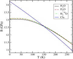
Figure 11: Bulk modulus as a function of temperature calculated with the TTM3-F force field model for H-ordered ice XI. Note that the anomalous isotope effect is recovered at $\sim$ 270 K.

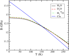
Figure 12: Bulk modulus as a function of temperature calculated with the TTM3-F force field model for H-disordered ice Ih. Note that the anomalous isotope effect is recovered at $\sim$ 200 K.

VI.3 Volume as a Function of Pressure in Clathrate Hydrate Structure I

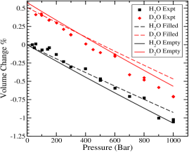
Figure 13: Volume change $V(P)/V_{\rm H_{2}O}$ as a function of pressure for filled and empty clathrate hydrates of structure I. Note that the isotope effect stays anomalous regardless of the filling of the clathrate sI, and the main difference is in the slope of $V(P)$, therefore reflected in the exact value of the corresponding bulk modulus.

In Fig. 13, we present the isotope effect as a volume change % relative to H₂O at $P=0$ bar, $V(P)/V_{\rm H_{2}O}$, for the filled clathrate structure as compared to the empty structure presented in Fig. 6 in the main paper. The isotope effect stays anomalous regardless of the existence of the host molecules, and the main difference is in the slopes of the $V(P)$ lines.

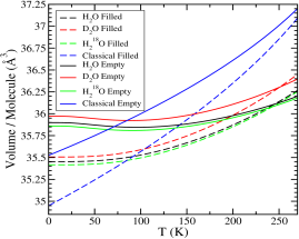
Figure 14: Volume per molecule as a function of temperature for filled and empty clathrate hydrate structure I. The solid lines are the empty structure and the dashed lines are the filled structure.

We present the empty clathrate sI results in the main paper for a fair comparison with the other ice structures. Here we also present the results for the clathrate hydrate structure I with 8 CH₄ host molecules.

Fig. 14 shows the volume per molecule as a function of temperature for the filled clathrate structure as compared to the empty structure presented in Fig. 7 in the main paper. Again the isotope effect is anomalous regardless of the host molecules. We also find that the volume per water molecule of the filled structure is smaller than that of the empty structure, in agreement with the experimental results on clathrates.

VI.4 Isotope Effect on the Volume of Ice VIII at High Pressure

Ice VIII is a stable phase under applied pressure. In Fig. 15, we present the volume per molecule as a function of temperature under applied pressure of $P=2.5$ GPa.

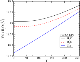
Figure 15: Volume per molecule as a function of temperature for ice VIII at $P=2.5$ GPa calculated with the QHA using the vdW-DF${\rm PBE}$ functional.

We compare the experimental volume per molecule $V=18.4$ Å  at $P=2.4$ GPa W. F. Kuhs and Bliss (1984) with the calculated volume of $V=19.06$ Å, and the calculated volume is slightly overestimated. The isotope effect on ice VIII stays normal up to the melting point regardless of the pressure.

References

- Kell (1967) G. S. Kell, Journal of Chemical & Engineering Data 12, 66 (1967).
- Smirnova et al. (2006) N. Smirnova, T. Bykova, K. V. Durme, and B. V. Mele, J. Chem. Thermodynamics 38, 879 (2006).
- Angell et al. (1973) C. A. Angell, J. Shuppert, and J. C. Tucker, J. Phys. Chem. 77, 3092 (1973).
- Kumar et al. (2008) P. Kumar, G. Franzese, and H. E. Stanley, J. Phys.: Condens. Matter 20, 244114 (2008).
- Mallamace et al. (2013) F. Mallamace, C. Corsaro, and H. E. Stanley, Proc. Nat. Acc. Sci. 110, 4899 (2013).
- Kumar and Stanley (2011) P. Kumar and H. E. Stanley, J. Phys. Chem. B 115, 14269 (2011).
- Sciortino et al. (2011) F. Sciortino, I. Saika-Voivod, and P. H. Poole, Phys. Chem. Chem. Phys. 13, 19759 (2011).
- Abascal and Vega (2011) J. L. F. Abascal and C. Vega, J. Chem. Phys. 134, 186101 (2011).
- Paschek (2004) D. Paschek, J. Chem. Phys. 120, 6674 (2004).
- Pi et al. (2009) H. L. Pi, J. L. Aragones, C. Vega, E. G. Noya, J. L. F. Abascal, M. A. Gonzalez, and C. McBride, Mol. Phys. 107, 365 (2009).
- Paschek (2005) D. Paschek, Phys. Rev. Lett. 94, 217802 (2005).
- Corradini et al. (2010) D. Corradini, M. Rovere, and P. Gallo, J. Chem. Phys. 132, 134508 (2010).
- Sciortino et al. (1997) F. Sciortino, P. H. Poole, U. Essmann, and H. E. Stanley, Phys. Rev. E 55, 727 (1997).
- Moore and Molinero (2011) E. B. Moore and V. Molinero, Nature 479, 506 (2011).
- Limmer and Chandler (2012) D. T. Limmer and D. Chandler, J. Chem. Phys. 137, 044509 (2012).
- Huang et al. (2009) C. Huang, K. T. Wikfeldt, T. Tokushima, D. Nordlund, Y. Harada, U. Bergmann, M. Niebuhr, T. M. Weiss, Y. Horikawa, M. Leetmaa, M. P. Ljungberg, O. Takahashi, A. Lenz, L. Ojamäe, S. S. A. P. Lyubartsev, L. G. M. Pettersson, and A. Nilsson, Proc. Nat. Acc. Sci. 106, 15214 (2009).
- Kaya et al. (2013) S. Kaya, D. Schlesinger, S. Yamamoto, J. T. Newberg, H. O. H. Bluhm, T. Kendelewicz, J. G. E. Brown, L. G. M. Pettersson, and A. Nilsson, Sci. Rep. 3, 1074 (2013).
- Pamuk et al. (2012) B. Pamuk, J. M. Soler, R. Ramirez, C. P. Herrero, P. W. Stephens, P. B. Allen, and M.-V. Fernandez-Serra, Phys. Rev. Lett. 108, 193003 (2012).
- Corsetti et al. (2013) F. Corsetti, M.-V. Fernández-Serra, J. M. Soler, and E. Artacho, J. Phys.: Condens. Matter 25, 435504 (2013).
- Kell (1977) G. S. Kell, J. Phys. Chem. Ref. Data 6, 1109 (1977).
- Ceriotti et al. (2016) M. Ceriotti, W. Fang, P. G. Kusalik, R. H. McKenzie, A. Michaelides, M. A. Morales, and T. E. Markland, Chemical Reviews 116, 7529 (2016).
- Franks (2000) F. Franks, Water - A Matrix of Life (Royal Society of Chemistry, 2000).
- Röttger et al. (1994) K. Röttger, A. Endriss, J. Ihringer, S. Doyle, and W. F. Kuhs, Acta Cryst. B50, 644 (1994).
- Allen (1994) P. B. Allen, Phil. Mag. B 70, 527 (1994).
- Habershon et al. (2009) S. Habershon, T. E. Markland, and D. E. Manolopoulos, J. Chem. Phys. 131, 024501 (2009).
- McKenzie et al. (2014) R. H. McKenzie, C. Bekker, B. Athokpam, and S. G. Ramesh, J. Chem. Phys. 140, 174508 (2014).
- Li et al. (2011) X.-Z. Li, B. Walker, and A. Michaelides, Proc. Nat. Acc. Sci. 108, 6369 (2011).
- Zeidler et al. (2011) A. Zeidler, P. S. Salmon, H. E. Fischer, J. C. Neuefeind, J. M. Simonson, H. Lemmel, H. Rauch, and T. E. Markland, Phys. Rev. Lett. 107, 145501 (2011).
- Markland and Berne (2012) T. E. Markland and B. J. Berne, Proceedings of the National Academy of Sciences 109, 7988 (2012).
- Romanelli et al. (2013) G. Romanelli, M. Ceriotti, D. E. Manolopoulos, C. Pantalei, R. Senesi, and C. Andreani, J. Phys. Chem. Lett. 4, 3251 (2013).
- Pamuk et al. (2015) B. Pamuk, P. B. Allen, and M.-V. Fernández-Serra, Phys. Rev. B 92, 134105 (2015).
- Koichiro Umemoto and Baroni (2010) S. d. G. Koichiro Umemoto, Renata M. Wentzcovitch and S. Baroni, Chemical Physics Letters 499, 236 (2010).
- Murray and Galli (2012) E. D. Murray and G. Galli, Phys. Rev. Lett. 108, 105502 (2012).
- Umemoto et al. (2015) K. Umemoto, E. Sugimura, S. de Gironcoli, Y. Nakajima, K. Hirose, Y. Ohishi, and R. M. Wentzcovitch, Phys. Rev. Lett. 115, 173005 (2015).
- Umemoto and Wentzcovitch (2017) K. Umemoto and R. M. Wentzcovitch, Japanese Journal of Applied Physics 56, 05FA03 (2017).
- Klapproth et al. (2003) A. Klapproth, E. Goreshnik, D. Staykova, H. Klein, and W. F. Kuhs, Canadian Journal of Physics 81, 503 (2003).
- Tajima et al. (1982) Y. Tajima, T. Matsuo, and H. Suga, Nature 299, 810 (1982).
- Blackman and Lisgarten (1958) M. Blackman and N. D. Lisgarten, Advances in Physics 7, 189 (1958).
- Svishchev and Kusalik (1994) I. M. Svishchev and P. G. Kusalik, Phys. Rev. Lett. 239, 349 (1994).
- Bertie et al. (1963) J. E. Bertie, C. L. D., and E. Whalley, J. Chem. Phys. 38, 840 (1963).
- Bertie and Whalley (1964) J. E. Bertie and E. Whalley, J. Chem. Phys. 40, 1646 (1964).
- Amaya et al. (2017) A. J. Amaya, H. Pathak, V. P. Modak, H. Laksmono, N. D. Loh, J. A. Sellberg, R. G. Sierra, T. A. McQueen, M. J. Hayes, G. J. Williams, M. Messerschmidt, S. Boutet, M. J. Bogan, A. Nilsson, C. A. Stan, and B. E. Wyslouzil, The Journal of Physical Chemistry Letters 8, 3216 (2017).
- Román-Pérez et al. (2010) G. Román-Pérez, M. Moaied, J. M. Soler, and F. Yndurain, Phys. Rev. Lett. 105, 145901 (2010).
- Wang et al. (2011) J. Wang, G. Roman-Perez, J. M. Soler, E. Artacho, and M.-V.Fernandez-Serra, J. Chem. Phys. 134, 024516 (2011).
- J.D et al. (1993) L. J.D, W. F. Kuhs, and J. L. Finney, J. Chem. Phys. 98, 4878 (1993).
- Kuhs et al. (1998) W. F. Kuhs, C. Lobban, and J. L. Finney, The Review of High Pressure Science and Technology 7, 1141 (1998).
- Whalley et al. (1968) E. Whalley, J. B. R. Heath, and D. W. Davidson, J. Chem. Phys. 48, 2362 (1968).
- Kamb (1964) B. Kamb, Acta Crystallographica 17, 1437 (1964).
- Kamb et al. (1971) B. Kamb, W. C. Hamilton, S. J. LaPlaca, and A. Prakash, J. Chem. Phys. 55, 1934 (1971).
- Whitworth and Petrenko (1999) R. W. Whitworth and V. F. Petrenko, “Physics of ice” (Oxford University Press, 1999).
- Salzmann et al. (2009) C. G. Salzmann, P. G. Radaelli, E. Mayer, and J. L. Finney, Phys. Rev. Lett. 103, 105701 (2009).
- James D. Jorgensen and Worlton (1984) N. W. James D. Jorgensen, R. A. Beyerlein and T. G. Worlton, J. Chem. Phys. 81, 3211 (1984).
- W. F. Kuhs and Bliss (1984) C. V. W. F. Kuhs, J. L. Finney and D. V. Bliss, J. Chem. Phys. 81, 3612 (1984).
- Nelmes et al. (1993) R. J. Nelmes, J. S. Loveday, R. M. Wilson, J. M. Besson, P. Pruzan, S. Klotz, and et. al., Phys. Rev. Lett. 71, 1192 (1993).
- Besson et al. (1994a) J. M. Besson, P. Pruzan, S. Klotz, G. Hamel, B. Silvi, R. J. Nelmes, and et. al., Phys. Rev. B 49, 12540 (1994a).
- Nelmes et al. (1998) R. J. Nelmes, J. S. Loveday, J. M. Besson, S. Klotz, and G. Hamel, The Review of High Pressure Science and Technology 7, 1138 (1998).
- Umemoto and Wentzcovitch (2004) K. Umemoto and R. M. Wentzcovitch, Phys. Rev. B 69, 180311 (2004).
- Umemoto and Wentzcovitch (2005) K. Umemoto and R. M. Wentzcovitch, Phys. Rev. B 71, 012102 (2005).
- J-C. Li and Eccleston (1999) A. I. K. J-C. Li, C. Burnham and R. S. Eccleston, Phys. Rev. B 59, 9088 (1999).
- Ziman (1979) J. M. Ziman, Principles of the Theory of Solids (Cambridge University Press, 1979).
- Ramírez et al. (2012) R. Ramírez, N. Neuerburg, M.-V. Fernández-Serra, and C. P. Herrero, J. Chem. Phys. 137, 044502 (2012).
- Salim et al. (2016) M. A. Salim, S. Y. Willow, and S. Hirata, The Journal of Chemical Physics 144, 204503 (2016).
- Allen (2015) P. B. Allen, Phys. Rev. B 92, 064106 (2015).
- Ordejón et al. (1996) P. Ordejón, E. Artacho, and J. M. Soler, Phys. Rev. B 53, 10441 (1996).
- Soler et al. (2002) J. M. Soler, E. Artacho, J. D. Gale, A. García, J. Junquera, P. Ordejón, and D. Sánchez-Portal, J Phys. Condens. Matter 14, 2745 (2002).
- Perdew et al. (1996) J. P. Perdew, K. Burke, and M. Ernzerhof, Phys. Rev. Lett. 77, 3865 (1996).
- Dion et al. (2004) M. Dion, H. Rydberg, E. Schröder, D. C. Langreth, and B. I. Lundqvist, Phys. Rev. Lett. 92, 246401 (2004).
- Román-Pérez and Soler (2009) G. Román-Pérez and J. M. Soler, Phys. Rev. Lett. 103, 096102 (2009).
- Fanourgakis and Xantheas (2008) G. S. Fanourgakis and S. S. Xantheas, J. Chem. Phys. 128, 074506 (2008).
- Santra et al. (2013) B. Santra, J. Klimeš, A. Tkatchenko, D. Alfè, B. Slater, A. Michaelides, R. Car, and M. Scheffler, The Journal of Chemical Physics 139, 154702 (2013).
- Pamuk (2014) B. Pamuk, Nuclear quantum effects in ice phases and water from first principles calculations, Ph.D. thesis, Stony Brook University (2014).
- Line and Whitworth (1996) C. M. B. Line and R. W. Whitworth, J. Chem. Phys. 104, 10008 (1996).
- Gagnon et al. (1988) R. E. Gagnon, H. Kiefte, M. J. Clouter, and E. Whalley, J. Chem. Phys. 89, 4522 (1988).
- Feistel and Wagner (2006) R. Feistel and W. Wagner, Journal of Physical and Chemical Reference Data 35, 1021 (2006).
- Hamada (2010) I. Hamada, J. Chem. Phys. 133, 214503 (2010).
- Gammon et al. (1983) P. H. Gammon, H. Klefte, and M. J. Clouter, The Journal of Physical Chemistry 87, 4025 (1983).
- Herrero and Ramírez (2011) C. P. Herrero and R. Ramírez, J. Chem. Phys 134, 094510 (2011).
- Ganeshan et al. (2013) S. Ganeshan, R. Ramírez, and M. V. Fernández-Serra, Phys. Rev. B 87, 134207 (2013).
- Lee et al. (2010) K. Lee, E. D. Murray, L. Kong, B. I. Lundqvist, and D. C. Langreth, Phys. Rev. B 82, 081101 (2010).
- Fortes et al. (2005) A. D. Fortes, I. G. Wood, M. Alfredsson, L. Vočadlo, and K. S. Knight, Journal of Applied Crystallography 38, 612 (2005).
- Gagnon et al. (1990) R. E. Gagnon, H. Kiefte, M. J. Clouter, and E. Whalley, The Journal of Chemical Physics 92, 1909 (1990).
- Klotz et al. (2017) S. Klotz, K. Komatsu, H. Kagi, K. Kunc, A. Sano-Furukawa, S. Machida, and T. Hattori, Phys. Rev. B 95, 174111 (2017).
- Ludl et al. (2017) A.-A. Ludl, L. E. Bove, D. Corradini, A. M. Saitta, M. Salanne, C. L. Bull, and S. Klotz, Phys. Chem. Chem. Phys. 19, 1875 (2017).
- Besson et al. (1994b) J. M. Besson, P. Pruzan, S. Klotz, G. Hamel, B. Silvi, R. J. Nelmes, J. S. Loveday, R. M. Wilson, and S. Hull, Phys. Rev. B 49, 12540 (1994b).
- Zhang et al. (2015) X. Zhang, P. Sun, T. Yan, Y. Huang, Z. Ma, B. Zou, W. Zheng, J. Zhou, Y. Gong, and C. Q. Sun, Progress in Solid State Chemistry 43, 71 (2015).
- Kittel (2005) C. Kittel, Introduction ot Solid State Physics (John Wiley & Sons, Inc., 2005).