Uncertainty in cardiac myofiber orientation and stiffnesses dominate the variability of left ventricle deformation response

Abstract.

Computational cardiac modelling is a mature area of biomedical computing, and is currently evolving from a pure research tool to aiding in clinical decision making. Assessing the reliability of computational model predictions is a key factor for clinical use, and uncertainty quantification (UQ) and sensitivity analysis are important parts of such an assessment. In this study, we apply new methods for UQ in computational heart mechanics to study uncertainty both in material parameters characterizing global myocardial stiffness and in the local muscle fiber orientation that governs tissue anisotropy. The uncertainty analysis is performed using the polynomial chaos expansion (PCE) method, which is a non-intrusive meta-modeling technique that surrogates the original computational model with a series of orthonormal polynomials over the random input parameter space. In addition, in order to study variability in the muscle fiber architecture, we model the uncertainty in orientation of the fiber field as an approximated random field using a truncated Karhunen-Loéve expansion. The results from the UQ and sensitivity analysis identify clear differences in the impact of various material parameters on global output quantities. Furthermore, our analysis of random field variations in the fiber architecture demonstrate a substantial impact of fiber angle variations on the selected outputs, highlighting the need for accurate assignment of fiber orientation in computational heart mechanics models.

1. Introduction

Computational modelling of the heart is a powerful technique for detailed investigations of cardiac behavior, and enables the study of mechanisms and processes that are not directly accessible by experimental methods. There is currently a drive towards adapting these computational models to individual patient data, to aid in the creation of individualized diagnosis, clinical decision support, and treatment planning [1, 2, 3, 4, 5, 6, 7]. However, this model adaptation presents a number of challenges related to the lack of available data and the fact that measurable data, needed for patient-specific model input parameters, are inherently subject to measurement uncertainties or intrinsic biological variability. For clinical use of models, it is therefore of crucial importance to quantify how these uncertainties propagate through the computational model to impact the output quantities of interest. Such assessment should be performed with uncertainty propagation and uncertainty quantification (UQ) techniques [8, 9], complemented by sensitivity analysis (SA) to identify the most significant input variables [10].

In the particular case of cardiac ventricular mechanics studies, individualized model adaption involves image-based construction of computational geometries as well as tuning of material parameters [11, 12, 13, 14, 15, 16, 17, 18]. Since the mechanical properties of cardiac tissue are strongly anisotropic, the local material behavior typically depends both on a set of material parameters and on the local orientation of the cardiac muscle cells, typically referred to as the fiber- and sheet orientation. The local tissue structure can be determined with diffusion tensor magnetic resonance imaging (DTMRI), but this technique is still limited to ex vivo experiments. Patient specific models have been created by projecting ex vivo DTMRI datasets onto patient-specific geometries obtained from computed tomography (CT) or magnetic resonance imaging (MRI) [19, 20, 21, 11, 22]. However, even in the in vitro case the accuracy of DTMRI is $\pm$ 10 degrees [23, 24, 25]. While this accuracy may be sufficient in the context of computational cardiac electrophysiology [26], local variations of this order have been shown to introduce sizeable variations in myofiber stresses [27].

Rule-based or atlas-based methods represent a convenient alternative for assigning fiber- and sheet orientation in patient specific models. For instance, the Laplace-Dirichlet Rule-Based (LDRB) algorithm [16] is based on atlas data, and assigns a generic tissue architecture to image-based patient-specific geometries. This method obviously neglects potential individual variations in tissue structure, but provides a reasonable averaged fiber/sheet orientation. Lombaert et al. [20] built the first statistical atlas of the cardiac fiber architecture using human datasets (10 ex vivo hearts imaged with DTMRI), providing the spatial distribution of fiber angles with their variability within the healthy population. Their results showed that the helix angle of the fibers varies globally from $-41^{\circ}$ ($\pm 26^{\circ}$) on the epicardium to $-66^{\circ}$ ($\pm 15^{\circ}$) on the endocardium. The reported variability includes both true variability of the fiber structure and errors due to acquisition and image registration. Similarly, Molléro et al. [28] estimated and represented the uncertainty of cardiac fiber architecture originating from the lack of data for a given patient using the mean and principal modes of variations among a given population of healthy hearts.

In spite of the potential impact for clinical use of the models, there are relatively few examples of proper UQ and SA for mechanical models of the heart. Osnes and Sundnes [29] and Hurtado et al. [30] studied the impact of uncertainty in material parameters, while Puijmert et al. [31] investigated the sensitivity of a cardiac mechanics model to changes in myofiber orientation over an average angle of about 8^∘. An increase in total pump work of 11-19 $\%$ was found in three different geometries, revealing that implementing an accurate fiber field is important for achieving the correct model output. Sensitivity of cardiac models to the myofiber orientation was also highlighted in [32, 18, 33].

One explanation for limited use of UQ and SA in cardiac modeling is the computational expense of the involved models. A popular statistical approach is the Monte Carlo (MC) method, but this method typically requires a large number of model evaluations for converged results. If the base model is a realistic computational model of cardiac mechanics, the resulting computational cost will be substantial. Techniques such as the quasi-Monte Carlo (QMC) [34, 35] and the multilevel Monte Carlo (MLMC) [36] methods can significantly improve the MC convergence rate, but their application may be limited and technically complex. Recently, alternative approaches, such as the use of surrogate models [37] to mimic the behaviour of the full model while being inexpensive to evaluate, have been of particular interest. One such technique is the polynomial chaos expansion method (PCE) [38, 39], which has previously been used in UQ analysis of cardiac mechanics and electrophysiology [29, 40].

The purpose of the present work is to present a PCE based method for UQ in cardiac mechanics models, and to perform an initial UQ and SA study including both global myocardial material properties and local variability of the microstructure orientation. The study of global material parameters is similar to the UQ analysis in [29], but using a more realistic computational model and including a detailed SA of key input- and output variables. The UQ considering local variations in microstructure orientation is, to our knowledge, the first of its kind. In this case, the input was treated as a random field, and modeled as a truncated Karhunen-Loève expansion (KLE) [41] in order to reduce the dimensionality of the random field representation. The former is used as a basis to build a reduced-dimensionality representation of the random field, essential to manage UQ analysis in extremely high-dimensional problems. Although the fiber arrangement exhibit a typical gross architecture, as we mention above, there are local and individual variations through the ventricular wall, as well as uncertainty derived from noisy measurements that may affect the global mechanical properties of the model. The results give insight into the applicability of the truncated KLE method for representing noisy fiber architecture fields, and to the impact of such variations on global response quantities.

2. Models and methods

The overarching objective of this paper is to illustrate and evaluate the impact of input data uncertainty on the mechanical response of the heart. We introduce the forward model for the mechanical behaviour of the left ventricle and its numerical approximation in Section 2.1 below and describe our UQ techniques subsequently in Section 2.2

2.1. Cardiac ventricular forward model

2.1.1. Governing equations

Let $D\subset\mathbb{R}^{3}$ be the computational domain representing the left ventricle. We consider the quasi-static and pressure-loaded mechanical equilibrium problem over this domain: find the displacement $\boldsymbol{u}:D\rightarrow\mathbb{R}^{3}$ such that

(1) $$-\nabla\cdot(\boldsymbol{FS})=0\quad\text{ in }D,$$

where $\boldsymbol{F}$ is the deformation gradient i.e. $\boldsymbol{F}=\nabla\boldsymbol{u}+\boldsymbol{I}$, and $\boldsymbol{S}$ is the second Piola-Kirchhoff stress tensor. Boundary conditions for (1) are described below.

We assume that the material is hyperelastic, and therefore that the Piola-Kirchhoff stress tensor $\boldsymbol{S}$ is the derivative of a strain energy density $\Psi=\Psi(\boldsymbol{E})$ with respect to the Green-Lagrange strain tensor $\boldsymbol{E}$, defined as

(2) $$\boldsymbol{E}=\frac{1}{2}\left(\boldsymbol{F}^{T}\boldsymbol{F}-\boldsymbol{I}\right).$$

In particular, we consider a transversely isotropic, hyperelastic and almost incompressible material, and apply the widely used constitutive model of Guccione et al. [42]. This model is defined relative to three mutually orthogonal vector fields: a fiber field $f:D\rightarrow\mathbb{R}^{3}$, a fiber sheet field $s:D\rightarrow\mathbb{R}^{3}$ and a sheet normal field $n:D\rightarrow\mathbb{R}^{3}$. The strain energy density is then defined as:

(3) $$\Psi(\boldsymbol{E})=\frac{1}{2}C(e^{W}-1)+K(J\ln J-J+1)$$

with

(4) $$W=b_{ff}E_{ff}^{2}+b_{xx}(E_{ss}^{2}+E_{nn}^{2}+E_{sn}^{2}+E_{ns}^{2})+b_{fx}(E_{fn}^{2}+E_{nf}^{2}+E_{fs}^{2}+E_{sf}^{2}).$$

Here, $E_{ij}$ are components of the Green-Lagrange strain tensor in the local fiber ($f$), fiber sheet ($s$), and sheet normal ($n$) axis, i.e. $E_{ij}=j\cdot\boldsymbol{E}i$ for directions $f$, $s$ and $n$. Additionally, $J$ is the determinant of the deformation gradient, and $C$, $K$, $b_{ff}$, $b_{xx}$ and $b_{fx}$ are material parameters. In particular, $b_{ff}$ and $b_{xx}$ are parameters governing the material stiffness in the fiber and cross-fiber directions, respectively, $b_{fx}$ represents the shear stiffness in planes parallel to the fibers, $K$ is the incompressibility factor of the myocardial tissue, and $C$ enters as a multiplicative factor in the strain energy function.

2.1.2. Geometry, mesh and fiber orientations

A computational mesh of the domain $D$ was generated from an echocardiographic image of a left ventricle at the beginning of atrial systole using the EchoPac software package (GE Healthcare Vingmed) and Gmsh. We constructed a flat ventricular base by cutting the geometry with a plane fit to the points on the base. The resulting linear tetrahedral volumetric mesh of the left ventricle wall is shown in Figure 1 (left), counting $4\,507$ vertices and $18\,112$ cells.

As note above, the model (3) assumes the availability of local coordinate systems $f,s,n$ aligned with the local orientation of muscle fibers. While the fiber orientation is not generally possible to measure in vivo, it is known that the fiber axes follow a helical pathway as illustrated in Figure 1 (right) with a counter-clockwise rotation of the helix angle from epicardium to endocardium [43]. In view of this, we applied a Laplace-Dirichlet Rule-Based (LDRB) algorithm [16] to generate realistic fiber-, fiber sheet- and sheet normal orientation fields in our ventricular model. The LDRB method defines two main angles to describe the local tissue structure. The fiber angle $\alpha$ defines the orientation of the longitudinal fiber direction relative to the circumferential direction, while $\beta$ is the angle between the transverse fiber direction and the outward transmural axis of the heart.

Input parameters to the model are the values of these angles on the endo- and epicardial surfaces, respectively: $\alpha_{endo}$, $\alpha_{epi}$, $\beta_{endo}$ and $\beta_{epi}$. Pointing ahead, in the present study we will both consider these input angles as random variables, as previously done in [29], and also apply a Karhunen-Loéve expansion (cf. Section 2.2.4) to study the impact of random variations in the full fiber field.

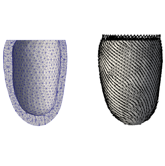
Figure 1. Left: computational mesh of a human left ventricle wall. Right: Baseline fiber orientation field $f$ over the computational mesh.

2.1.3. Boundary conditions

Following e.g. [44], to constrain the displacement at the base of the left ventricle boundary, we applied a Robin boundary condition with a spring constant of $1$ kPa. Moreover, we let the base of the left ventricle be clamped (zero displacement) in the longitudinal direction. At the endocardium (inner) surface, we applied a pressure of $2$ kPa, corresponding to the end-diastolic pressure, as a normal stress boundary condition. At the epicardium (outer) surface, we assumed zero normal stress.

2.1.4. Numerical discretization

To solve (1) with the previously described boundary conditions, we considered a finite element discretization. The fiber-, fiber sheet-, and sheet normal orientation fields were interpolated onto continuous piecewise linear vector fields defined relative to the computational mesh, and we similarly approximated the displacement field using continuous piecewise linear vector fields. The nonlinear systems of equations were solved using Newton’s method and the resulting linear equations were solved using a direct method. The endocardial pressure was applied incrementally to improve the nonlinear convergence.

2.2. Uncertainty quantification

For brevity, in the presentation of the UQ techniques, we will denote the finite element discretization of the forward model described by (1) and associated boundary conditions by $\mathscr{Y}$. In general, this forward model can be viewed as a function, over the space $\boldsymbol{x}\in D$, mapping a set of input parameters $\boldsymbol{\eta}$ to output values $Y$:

(5) $$Y=\mathscr{Y}(\boldsymbol{x},\boldsymbol{\eta}).$$

The mapping $\mathscr{Y}$ is deterministic, so that when evaluated on the same $d$ input parameters ${\boldsymbol{\eta}}=(\eta_{1},\dots,\eta_{d})$ it yields the same specific output values $Y$.

We will consider both the case where each $\eta_{i}$ represents a (single) random variable and the case where some $\eta_{i}$ represent a random field. Concretely, $\boldsymbol{\eta}$ will represent ventricular material parameters such as $C,K,b_{ff},b_{fx},b_{xx}$ and the input parameters of the fiber field model $\alpha_{endo},\alpha_{epi},\beta_{endo},\beta_{epi}$, or variables associated with the uncertainty in the orientation field $f$.

A UQ analysis evaluates the impact in output $Y$ that results from the uncertainty in the parameters $\boldsymbol{\eta}$, assuming a known joint probability distribution $p_{\boldsymbol{\eta}}$ associated with the input vector $\boldsymbol{\eta}$. The most popular technique for UQ analysis is MC simulation, which involves the use of a sampling method to draw a set of samples from the parameter space. Relevant statistics of the output $Y$ is obtained by evaluating the deterministic model (5) on the sampling set. Although simple and widely applicable, the MC technique converges slowly, and typically requires a large number of evaluations of the forward model $\mathscr{Y}$. In our case each evaluation involves solving a non-linear finite element model, leading to a substantial computational cost. We have therefore considered alternative techniques to reduce the required number of $\mathscr{Y}$ evaluations.

2.2.1. Polynomial Chaos Expansion

The Polynomial Chaos expansion (PCE) method [38] expands the uncertain model outputs in a suitable series, which mimics the behaviour of the forward model (5) but is much cheaper to evaluate. This series expansion can then be used to perform cheap UQ and SA, using sampling techniques such as the QMC method [34, 35]. In PCE, evaluations of the forward model (5) are required to build the series expansion, but the number of required model evaluations is normally lower than for standard sampling methods.

Assuming that the output of interest from (5) is a smooth function of $d$ random input parameters $\boldsymbol{\eta}=(\eta_{1},\dots,\eta_{d})$, the PCE approximates $Y$ as a function of $\boldsymbol{\eta}$ by a truncated polynomial expansion as follows [45]:

(6) $$Y(\boldsymbol{x},\boldsymbol{\eta})\approx\hat{Y}(\boldsymbol{x},\boldsymbol{\eta})=\sum_{i=1}^{M}c_{i}(\boldsymbol{x})\Phi_{i}(\boldsymbol{\eta}).$$

Here, $\{\Phi_{i}\}$ is a given multivariate orthogonal polynomial basis for $\boldsymbol{\eta}$, $c_{i}(\boldsymbol{x})$ are the coefficients that quantify the dependence of the model output on the parameters $\boldsymbol{\eta}$, and $M$ is the total number of expansion terms. This number is determined by the dimension $d$ of the random vector $\boldsymbol{\eta}$ and the highest order $N$ of the polynomials $\{\Phi_{i}\}$, more precisely $M=(N+d)!\,(N!\,d!)^{-1}$. The deterministic functions $c_{i}(\boldsymbol{x})$ may be computed by the point collocation method [46]. Within this technique, the unknown coefficients of the expansion are estimated by equating model outputs and the corresponding polynomial chaos expansion at a set of collocation points in the parameter space. For each output of the model, a set of linear equations is formed with the coefficients as the unknowns:

(7) $$\begin{pmatrix}\Phi_{1}(\boldsymbol{q}_{1})\ &\cdots&\Phi_{M}(\boldsymbol{q}_{1})\\ \vdots&\ddots&\vdots\\ \Phi_{1}(\boldsymbol{q}_{N_{s}})&\cdots&\Phi_{M}(\boldsymbol{q}_{N_{s}})\\ \end{pmatrix}\begin{pmatrix}c_{1}(\cdot)\\ \vdots\\ c_{M}(\cdot)\\ \end{pmatrix}=\begin{pmatrix}\mathscr{Y}(\cdot,\boldsymbol{q}_{1})\\ \vdots\\ \mathscr{Y}(\cdot,\boldsymbol{q}_{N_{s}})\\ \end{pmatrix}$$

The collocation points $\{\boldsymbol{q}_{1},\dots\boldsymbol{q}_{N_{s}}\}$ must be chosen in a way so that the matrix (7) is well-conditioned [47]. This requirement allows for the use of conventional QMC sampling methods [48] to select a number of collocation points equal or greater than the number of unknown coefficients $c_{i}(\boldsymbol{x})$ [46].

Once the coefficients are determined and $\hat{Y}(\boldsymbol{x},\boldsymbol{\eta})$ is built, the last step in the PCE method for UQ is to propagate the uncertainties through the simulator in order to estimate statistics of the response quantities. This last step is performed by MC simulations, in which the model solver of (5) is substituted by the surrogate $\hat{Y}$ as a cheaper alternative. It is important to note that for PCE, the convergence depends on both the maximal order $N$ of the polynomials $\{\Phi_{i}\}$ and the number of collocation points $N_{s}$ selected to build $\hat{Y}$. We return to this point in Section 3. Typical statistical response quantities include expected value ($\mu$), standard deviation ($\sigma$), prediction intervals and coefficient of variation, in order to characterize the probability density function (pdf) corresponding to each output quantity of interest [49].

2.2.2. QMC

We have also applied Quasi-Monte Carlo (QMC) [34, 35] simulations with Halton low-discrepancy sampling sequences [50] to verify and validate the results obtained by the PCE methods.

2.2.3. Sobol sensitivity indices

In addition to computing statistical properties of the output probabilities, we perform SA [51, 10, 52] to quantify the contribution of a particular input $\eta_{i}$, and of specific parameter interactions, to the output variance. This analysis may be useful for model personalization, for which input fixing (identify non-influential parameters to fix them within their uncertainty domain) and input prioritization (determination of which factor(s), once fixed to its true value, leads on average to the greatest reduction in the variance of an output) are important goals. In this study we compute the total ($S_{i}^{T}$) and the main ($S_{i}$) variance-based Sobol sensitivity indices [53], which can be used for input fixing and input prioritization, respectively.

Specifically, the main sensitivity index $S_{i}$ is the proportion of the total variance $\mathbb{V}$ of $Y$ that is expected to be reduced if $\eta_{i}$ was fixed on its unknown true value. It can be computed according to [54]:

(8) $$S_{i}=\frac{\mathbb{V}[\mathbb{E}[Y|\eta_{i}]]}{\mathbb{V}[Y]},$$

where the index $i$ varies from 1 to the number of random inputs $d$, and $\mathbb{E}$ is the expected value of the output quantity in question $Y$. Furthermore, the total sensitivity index $S_{i}^{T}$, which represents the total variance due to both the direct effect and all input interactions of $\eta_{i}$, is given by [54]:

(9) $$S_{i}^{T}=\frac{\mathbb{V}[Y]-\mathbb{V}[\mathbb{E}[Y|\boldsymbol{\eta}_{i*}]]}{\mathbb{V}[Y]}$$

in which $\boldsymbol{\eta}_{i*}$ contains all uncertain inputs except $\eta_{i}$.

2.2.4. Karhunen-Loève expansion

One of the key goals of this paper is to quantify and evaluate the impact of uncertainty originating from the variability of the myofiber orientation field $f$ cf. (4). As a statistical model for an input which address variability as function of space, it must be described by a random field variable. In particular, in the following we will consider a random myofiber orientation field as the sum of a random field perturbation and a fiber field generated by the LDRB method of Bayer et al. [16].

(10) $${}f(\boldsymbol{x},\theta)=f_{LDRB}(\boldsymbol{x})+F(\boldsymbol{x},\theta),\quad\boldsymbol{x}\in D,$$

where $\theta\in\Omega$ denotes the dependency of $f$ on some random property. To represent the random field perturbation, we make use of a truncated Karhunen-Loéve expansion. Any second-order random field $F(\boldsymbol{x},\theta)$ defined over $D\times\Omega$, with covariance function $C$ and expected value $\bar{F}$, can be represented by the Karhunen-Loéve expansion [41, 55], also known as the proper orthogonal decomposition, as the following infinite linear combination of orthogonal functions:

(11) $$F(\boldsymbol{x},\theta)=\bar{F}(\boldsymbol{x})+\sum_{k=1}^{\infty}\eta_{k}(\theta)\sqrt{\lambda_{k}}\phi_{k}(\boldsymbol{x}).$$

In (11), $\bar{F}(\boldsymbol{x})$ is the expected value of the stochastic field at $\boldsymbol{x}$, $\{\eta_{k}(\theta)\}$ represents a set of uncorrelated random variables (if $F(\boldsymbol{x},\theta)$ is assumed to be Gaussian then $\{\eta_{k}(\theta)\}$ are also independent), and $\{\lambda_{k}$, $\phi_{k}(\boldsymbol{x})\}$ are eigenvalues and eigenfunction pairs of the homogeneous Fredholm integral equation over $D$:

(12) $$\int_{D}C(\boldsymbol{y},\boldsymbol{x})\,\phi_{i}(\boldsymbol{y})\,{\rm{d}\boldsymbol{y}}=\lambda_{i}\phi_{i}(\boldsymbol{x}),$$

using the covariance function $C(\boldsymbol{y},\boldsymbol{x})$ as kernel [55].

In practice, the infinite series in (11) may be truncated after the terms corresponding to the highest $n_{\rm KL}$ eigenvalues $\{\lambda_{k}\}$:

(13) $${}F(\boldsymbol{x},\theta)\approx\tilde{F}(\boldsymbol{x},\theta)=\bar{F}(\boldsymbol{x})+\sum_{k=1}^{n_{\rm KL}}\eta_{k}(\theta)\sqrt{\lambda_{k}}\phi_{k}(\boldsymbol{x}).$$

The number of terms $n_{\rm KL}$ depends on the decay of eigenvalues, which in turn depends on the smoothness of the covariance function $C$. If the eigenvalues $\{\lambda_{k}\}$ decay sufficiently fast and $n_{\rm KL}$ is large enough, $\tilde{F}$ provides a suitable approximation of $F$.

In this study, as we consider a random field perturbation to the myofiber orientations, we assume $\bar{F}(\boldsymbol{x})=0$, without loss of generality. Moreover, we have chosen the squared exponential covariance structure  [56] as the covariance function;

(14) $$C(\boldsymbol{x},\boldsymbol{y})=\sigma_{\rm KL}^{2}\exp(-\frac{|\boldsymbol{x}-\boldsymbol{y}|^{2}}{2l^{2}})\hskip 28.45274pt\forall\,\boldsymbol{x},\boldsymbol{y}\in D.$$

Here $\sigma_{\rm KL}^{2}$ is the field variance controlling the typical amplitude of the random field, and $l$ is the correlation length that defines the typical length-scale over which the field exhibits significant correlations. Considering the lack of experimental data from which to estimate the spatial uncertainty associated to the myofiber orientation field, we consider this choice of correlation function to be a sensible starting point for study. Finally, in this study, the approach of truncation has been to examine the decay of the eigenvalues $\{\lambda_{k}\}$ in (11) and keep the first $n_{\rm KL}$ eigenvalues $\{\phi_{k}(\boldsymbol{x})\}$ so that the contributions from the remaining eigenvalues are negligible.

This reduction of dimensionality of the stochastic space, from infinite to $n_{\rm KL}$, provides a parametric representation of the random field $F(\boldsymbol{x},\theta)$ through $n_{\rm KL}$ random variables. The uncertainty of the fiber field now stems from the vector of parameters ${\boldsymbol{\eta}}=(\eta_{1},\dots,\eta_{\rm KL})$, with $\{\eta_{k}\}$ the uncorrelated random variables defined in (11). Standard uncertainty propagation methods, like MC or PCE, can be used then to predict the influence of the variability of the myofiber orientation (10) on our model. As an error measure for the random field truncation (13), we have used the error variance introduced by Betz et al. [57]. In particular, $n_{\rm KL}$ has been selected ensuring that in more than the $92\%$ of the discretized points $\boldsymbol{x}$, the error variance is lower than 0.05. In our experiments, $n_{\rm KL}$ range from $4$ to $16$ depending on the correlation length $l$ in (14).

2.2.5. Computing Karhunen-Loéve approximation

Analytical solutions of the eigenvalue problem (12) rarely exist, so in general it has to be solved numerically [58, 59]. For this purpose, we consider the weak formulation (Galerkin projection) of the system of equations (12) on a discretization of the domain $D$. In particular, assume that we have a mesh $\mathcal{T}_{h}$ of the fixed domain $D$ with vertices (nodes) $x_{1}\dots,x_{n}$. Take a continuous piecewise linear basis $\{v_{1},\dots,v_{n}\}$ defined relative to this mesh, and consider the generalized eigenvalue problem [60]: find $\phi_{k}$ and $\lambda_{k}$ such that

(15) $$T\phi_{k}=\lambda_{k}M\phi_{k},$$

where $M$ is the mass matrix:

(16) $$M_{ij}=\int_{D}v_{i}(\boldsymbol{x})v_{j}(\boldsymbol{x})\,{\rm d\boldsymbol{x}},$$

and

(17) $$T=MQM$$

with $Q_{ij}=C(\boldsymbol{x}_{i},\boldsymbol{x}_{j})$ the covariance matrix that emerges from the discrete representation of the random field with covariance kernel $C$.

It is important to note that while the mass matrix $M$ is symmetric positive definite and may be sparse, $T$ is symmetric positive semi-definite and dense. Since $Q$ is dense, we applied a data sparse technique to store it with the Hierarchical matrix ($\mathcal{H}$-matrix) format [60, 61]. Consequently, the computational cost of matrix-vector products involving $Q$ is reduced from $\mathcal{O}(n^{2})$ to $\mathcal{O}(n\log{}n)$, with $n$ the number of discretization points. The $\mathcal{H}$-matrix technique is a hierarchical division of a given matrix into rectangular blocks and further approximation of these blocks by low-rank matrices [62, 63, 64]. In order to compute the low-rank approximations, the Adaptive Cross Approximation (ACA) algorithm [65] was employed.

2.2.6. Statistical properties of random input quantities

Table 1. Statistical properties of the input parameters in Model A: probability distribution ($\rho_{\eta_{i}}$), expected value ($\mu_{\eta_{i}}$) and standard deviation ($\sigma_{\eta_{i}}$).

Parameter	Unit	$\rho_{\eta_{i}}$	$\mu_{\eta_{i}}$	$\sigma_{\eta_{i}}$
$b_{ff}$		Normal	6.6	0.99
$b_{xx}$		Normal	4.0	0.6
$b_{fx}$		Normal	2.6	0.39
$K$	kPa	Log-Normal	10.0	1.5
$C$	kPa	Log-Normal	1.1	0.165
$\alpha_{endo}$	degree	Normal	50.0	7.5
$\alpha_{epi}$	degree	Normal	40.0	6.0
$\beta_{endo}$	degree	Normal	65.0	9.75
$\beta_{epi}$	degree	Normal	25.0	3.75

In this study, we introduce two different models of uncertainty. First, we consider the material stiffnesses $b_{ff},b_{xx},b_{fx}$, the incompressibility parameter $K$ and the weighting factor $C$ as uncertain (random) variables of prescribed probability distributions. The statistical properties for these material parameters were chosen as in [29]. Moreover, we similarly treat randomness in fiber orientations as a direct function of the random input variables $\alpha_{endo}$, $\alpha_{epi}$, $\beta_{endo}$ and $\beta_{epi}$ to the LDRB algorithm. For these variables, we have assumed a normal distribution with expected values following [19] and a coefficient of variation equals to 0.15. The prescribed distributions, expected values and standard deviations are listed in Table 1, and we refer to this case as Model A. All parameters are treated as independent.

In the second model (Model B), we introduce uncertainty in the fiber orientation field only by adding a Gaussian random field to the fiber architecture generated by the LDRB algorithm. We thus introduce a non-uniform perturbation in angle orientation of every fiber axis over the computational geometry. The random perturbation field is approximated via the truncated Karhunen-Loéve expansion as described in Section 2.2.4. The properties of the random field depend strongly on the selected correlation length. We have considered three different correlation lengths: $l=3,5$ or $10$ cm, and two different standard deviations, $\sigma_{\rm KL}=0.1$ and 0.5 radians, respectively. In this second model (Model B), the five material parameters $C,K,b_{ff},b_{fx},b_{xx}$ and the angles $\alpha_{endo},\alpha_{epi},\beta_{endo},\beta_{epi}$ are kept fixed at their mean value given by Table 1.

Three samples of the different (total) random fiber orientation fields, $f(\boldsymbol{x},\theta)$ in (10) assuming a standard deviation of 0.5 radians, are illustrated in Figure 2. Note that short correlation lengths in the random field generates strong fluctuations in the fiber architecture, while a higher value of $l$ implies that the random field approaches a random variable (i.e. constant over the computational domain). The required number of terms $n_{\rm KL}$ in the Karhunen-Loéve decomposition (13) varies from 4, 9, and 16 with decreasing $l$, so the more correlated the orientation field, the smaller the number of terms necessary to retain its essential information in the truncated Karhunen-Loéve expansion.

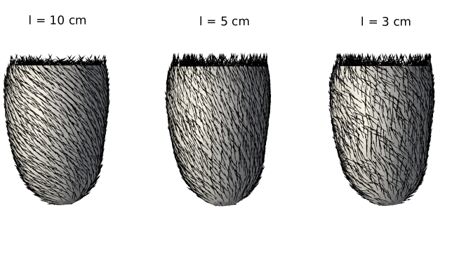
Figure 2. Samples of random fiber orientation fields (Model B), $f(\boldsymbol{x},\theta)$ in (10), generated by a Gaussian random field with a standard deviation $\sigma_{\rm KL}=0.5$ radians and correlation length equals $l=10$ cm (left), $l=5$ cm (middle) and $l=3$ cm (right).

2.2.7. Quantities of interest

As quantities of interest (or target values) we have chosen global, observable quantities: the volume of the inner cavity $Q_{c}$, the lengthening of the apex $Q_{l}$ (difference between epicardial and endocardial axial length), the change in wall thickness $Q_{t}$ (difference between outer and inner radius at base), and the total wall volume $Q_{v}$. The reference values of these quantities of interest (corresponding to the reference configuration of the ventricular domain at zero endocardial pressure) are given in Table 2.

Table 2. Quantities of interest corresponding to the reference configuration of the ventricular domain.

Quantity of interest (unit)	Reference value
Inner cavity volume $Q_{c}$ ($10^{2}$ $\times$ $\rm cm^{3}$)	1.70
Apex lengthening $Q_{l}$ ($\rm cm$)	1.11
Wall thickness $Q_{t}$ ($10^{-1}$ $\rm cm$)	6.99
Wall volume $Q_{v}$ ($10^{2}$ $\times$ $\rm cm^{3}$)	1.26

2.3. Implementation

We used the Python interface to the FEniCS finite element software [66, 67] to implement the forward model described in Section 2.1. The UQ analysis was performed using the ChaosPy toolbox [68], using the FEniCS forward solver as a black box model. We also used FEniCS to assemble the matrices $T$ and $M$ in (15). Finally, the dominant eigenmodes of the eigenvalue problem (15) (approximating the eigenmodes of (12)) were obtained using ARPACK accessed via SciPy [69].

3. Results

The main focus of this work is to quantify the impact of uncertainty in local myofiber architecture on representative global response quantities of interest. Prior to the main study focusing on model A and B as described above, we present results from the calibration of the surrogate PCE models.

3.1. Surrogate model calibration and validation of statistical outputs

The PCE model depends on the polynomial order $N$ ($\leq 3$) and number of sampling points $N_{s}$ ($\leq 4\times M$) used to fit the surrogate model to the finite element model. In order to choose these parameters, for each of the experiments below, we conducted a series of experiments ultimately choosing the $N$ and $N_{s}$ with the minimal mean-square error between the surrogate and the forward (finite element) model outputs for a new/different set of points in the parameter space.

Moreover, an extra convergence test has been performed comparing the standard deviation of every response quantity obtained via this validated single surrogate model with the same magnitude extracted from a QMC simulation through the Halton low-discrepancy sampling sequence. The results are included in Tables 3 and 4–5. Overall, the non-intrusive PCE method was able to successfully generate a surrogate model for each quantity of interest specified in Table 2.

3.2. Impact of input variable uncertainty

We first consider a UQ analysis of Model A, in particular of the nine model input random variables listed in Table 1 and the four output quantities of interest listed in Table 2. We computed statistical properties of the probability density functions associated with these output quantities, including mean value $\mu$, standard deviation $\sigma$, coefficient of variation $\sigma/\mu$ and the 95$\%$ prediction interval for each output quantity. The resulting statistical quantities are listed in Table 3 and the output density functions are depicted in Figures 3–4 (left panels). We observe that all coefficients of variation are at or below $0.08$, with the largest coefficient of variation associated with the inner cavity volume, and the smallest with the wall volume.

Table 3. Model A: Statistical properties of the quantities of interest probability densities: expected value ($\mu$), standard deviation ($\sigma$), coefficient of variation (cov = $\sigma/\mu$), and prediction interval (PI₉₅) via PCE. Standard deviation extracted from QMC simulations is also included (QMC).

Quantity	$\mu$	$\sigma$ (QMC)	cov	PI95
Inner volume ($10^{2}$ $\times$ $\rm cm^{3}$)	3.81	0.30 (0.30)	0.08	[3.23, 4.39]
Lengthening ($\rm cm^{3}$)	0.83	0.05 (0.05)	0.06	[0.73, 0.93]
Wall thickness ($10^{-1}$ $\rm cm^{3}$)	4.79	0.28 (0.27)	0.06	[4.24, 5.34]
Wall volume ($10$ $\times$ $\rm cm^{3}$)	9.83	0.43 (0.42)	0.04	[8.90, 10.7]

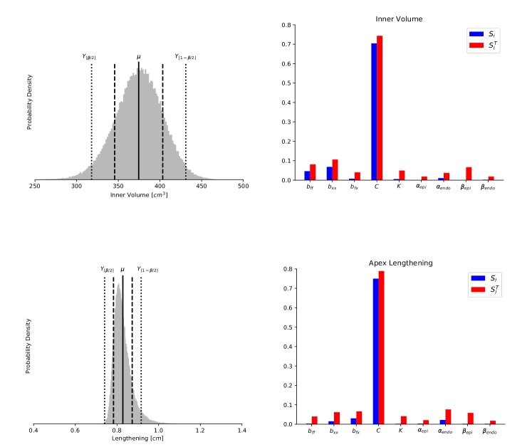
Figure 3. Model A: Probability density (left column) of the inner cavity volume (top) and apex lengthening (bottom) obtained assuming material input parameters included in Table 1. In vertical bars, the mean (solid line), mean $\pm$ standard deviation respectively (dashed lines), and the limits of the 95$\%$ prediction interval (dotted lines) are shown. Main Sobol’ index ($S_{i}$, blue) and total Sobol’ index ($S_{i}^{T}$, red) are depicted in right column for all quantities of interest.

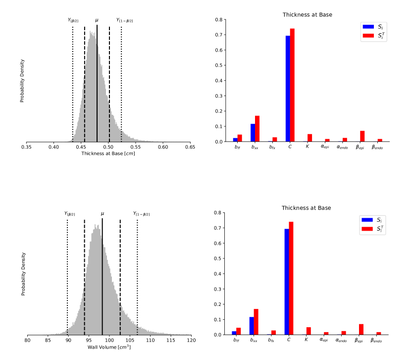
Figure 4. Model A: Probability density (left column) of the wall thickness at base (top) and wall volume (bottom) obtained assuming material input parameters included in Table.1. In vertical bars, the mean (solid line), mean $\pm$ standard deviation respectively (dashed lines), and the limits of the 95$\%$ prediction interval (dotted lines) are shown. Main Sobol’ index ($S_{i}$, blue) and total Sobol’ index ($S_{i}^{T}$, red) are depicted in the right columns for all quantities of interest.

For verification purposes, we also compared the resulting standard variation values with values obtained using QMC directly (without the use of the surrogate PCE model), also listed in Table 3. We observe that the discrepancy in the standard deviation between the PCE and the QMC simulations are less than $2\%$ for all output quantities.

From Figures 3–4, we observe that output density distributions display a high degree of symmetry (skewness $\sim$ 0), though with a certain distortion to the right in the case of the apex lengthening especially, but also for the thickness and wall volume, and slightly negatively skewed data in the case of the inner cavity volume.

In addition to the statistical properties reported in Table 3, we computed the main and total Sobol indices with respect to the input random variables for each output quantity. The indices are plotted in Figure 3–4 (right panels) in conjunction with the respective output quantities. Clearly, the uncertainty in the multiplicative factor $C$ has the highest main sensitivity index $S_{C}$ for all four output quantities, with $S_{c}\geq 0.6$ for all four cases. More precisely, these sensitivity indices indicate that if $C$ was known and fixed to its true value, then the uncertainty in the four output quantities $Q_{c},Q_{l},Q_{t}$, and $Q_{v}$ would be reduced by 70$\%$, 75$\%$, 69$\%$ and 61$\%$, respectively.

For the inner cavity volume, wall thickness, and wall volume, the material stiffness parameters $b_{ff}$ and $b_{xx}$ have main sensitivity index in the range $0.02-0.15$, with $b_{xx}$ having higher index than $b_{ff}$ in the case of thickness at base, while $b_{ff}$ have higher index than $b_{xx}$ in the case of wall volume and inner cavity volume. In particular, $b_{xx}$ yields a main sensitivity index greater than $0.05$ in the cases of inner cavity volume and thickness and thus emerges as a key parameter for these output quantities. Similarly, $b_{ff}$ emerges as a key parameter for the wall volume. For these output quantities, the main sensitivity index for the other variables ($b_{fx}$, $K$, $\alpha_{epi}$, $\alpha_{endo}$, $\beta_{epi}$, $\beta_{endo}$) essentially vanish. For the apex lengthening, we observe that the main sensitivity indices associated with $b_{fx}$, $b_{xx}$, and $\alpha_{endo}$ are small but non-vanishing, while the main sensitivity index associated with other variables ($b_{ff}$, $K$, $\alpha_{epi}$, $\beta_{epi}$, $\beta_{endo}$) essentially vanishes. Overall, the direct contributions of the angles $\alpha_{epi}$, $\beta_{endo}$ and $\beta_{epi}$ to the total variance of any output of interest are negligible: the main sensitivity index of all three angles is close to zero for for all the model outputs.

The total-order sensitivity indices identify the input variables that may be fixed over their range of variability without affecting some specific output variance. Indeed, these are those inputs corresponding to $S_{i}^{T}\simeq 0$ for all the quantities of interest [10, 9]. We observe that the angles $\alpha_{epi}$ and $\beta_{endo}$ satisfy this condition. These input parameters have the smallest total sensitivity indices for all the output quantities, and in particular, these inputs could be fixed in subsequent model calibrations within their range of uncertainty introducing only about $2\%$ of the current output variances. Finally, the total and main sensitivity indices are of similar value for all input parameters, which indicates no significant high-order interaction between the model inputs.

3.3. Impact of fiber field uncertainty

We next turn to consider a UQ analysis of Model B, where the local fiber orientation is modeled as a Gaussian random field. We consider a total of six cases; combining standard deviations $\sigma_{\rm KL}$ of 6.0 degrees (0.1 radians) and 28.6 degrees (0.5 radians) with correlation lenghts 3, 5, and 10 cm. The chosen standard deviation values are based on fiber angle variabilities reported in the literature, which include either measurement errors or a combination of measurement error and biological variations. Samples of the resulting random fields are illustrated in Figure 2. For all six cases, we computed statistical properties of the probability density functions associated with these global response quantities, including the mean value $\mu$, standard deviation $\sigma$, coefficient of variation $\sigma/\mu$ and the 95$\%$ prediction interval for each output quantity listed in Table 2. Statistical measures are presented in Tables 4–5, while the probability density functions are illustrated in Figures  5–6 for the inner volume and the wall thickness, as most relevant output quantities of interest.

For verification purposes, we also compared the resulting standard variation values with values obtained using QMC directly (without the use of the surrogate PCE model), also listed in Tables 4–5. We observe that the discrepancy in the standard deviation between the PCE and the QMC simulations is small, typically of the order $1-3\%$ for the range of output quantities and perturbation fields examined.

Table 4. Model B: Statistical properties of the output quantities distributions: expected value ($\mu$), standard deviation ($\sigma$), coefficient of variation (cov = $\sigma/\mu$), and prediction interval (PI₉₅). Gaussian random fields with a standard deviation $\sigma_{\rm KL}=0.1$ radians and correlation length $l$ equals to 3, 5 and 10 cm. Standard deviation extracted from QMC simulations is also included (QMC).

$l$ (cm)	Quantity	$\mu$	$\sigma$ (QMC)	cov ($\sigma/\mu$)	PI95
10	Inner volume ($10^{2}$ $\times$ $\rm cm^{3}$)	3.97	0.06 (0.06)	0.01	[2.79,5.15]
	Lengthening ($\rm cm$)	0.82	0.03 (0.03)	0.03	[0.76,0.89]
	Wall thickness ($10^{-1}$ $\times$ $\rm cm$)	4.75	0.03 (0.03)	0.006	[4.69,4.81]
	Wall volume ($10$ $\times$ $\rm cm^{3}$)	9.84	0.08 (0.09)	0.008	[9.68,9.99]
5	Inner volume ($10^{2}$ $\times$ $\rm cm^{3}$)	3.97	0.05 (0.05)	0.01	[3.87,4.07]
	Lengthening ($\rm cm$)	0.82	0.02 (0.02)	0.02	[0.78,0.86]
	Wall thickness ($10^{-1}$ $\times$ $\rm cm$)	4.75	0.02 (0.02)	0.004	[4.71,4.79]
	Wall volume ($10$ $\times$ $\rm cm^{3}$)	9.84	0.07 (0.07)	0.007	[9.70,9,98]
3	Inner volume ($10^{2}$ $\times$ $\rm cm^{3}$)	3.97	0.04 (0.04)	0.01	[3.89,4.05]
	Lengthening ($\rm cm$)	0.82	0.02 (0.02)	0.02	[0.78,0.86]
	Wall thickness ($10^{-1}$ $\times$ $\rm cm$)	4.75	0.02 (0.02)	0.004	[4.71,4.79]
	Wall volume ($10$ $\times$ $\rm cm^{3}$)	9.84	0.05 (0.05)	0.005	[9.74,9.94]

Table 5. Model B: Statistical properties of the output quantities distributions: expected value ($\mu$), standard deviation ($\sigma$), coefficient of variation (cov = $\sigma/\mu$), and prediction interval (PI₉₅). Gaussian random fields with a standard deviation $\sigma_{\rm KL}=0.5$ radians and correlation length $l$ equals to 3, 5 and 10 cm. Standard deviation extracted from QMC simulations is also included (QMC).

$l$ (cm)	Quantity	$\mu$	$\sigma$ (QMC)	cov ($\sigma/\mu$)	PI95
10	Inner volume ($10^{2}$ $\times$ $\rm cm^{3}$)	4.03	0.18 (0.17)	0.04	[3.70, 4.36]
	Lengthening ($\rm cm$)	0.78	0.06 (0.06)	0.08	[0.66, 0.90]
	Wall thickness ($10^{-1}$ $\times$ $\rm cm$)	4.70	0.05 (0.06)	0.01	[4.60, 4.82]
	Wall volume ($10$ $\times$ $\rm cm^{3}$)	9.66	0.18 (0.17)	0.02	[9.31, 10.0]
5	Inner volume ($10^{2}$ $\times$ $\rm cm^{3}$)	4.15	0.18 (0.17)	0.04	[3.80, 4.50]
	Lengthening ($\rm cm$)	0.77	0.05 (0.05)	0.07	[0.67, 0.87]
	Wall thickness ($10^{-1}$ $\times$ $\rm cm$)	4.64	0.09 (0.09)	0.02	[4.47, 4.81]
	Wall volume ($10$ $\times$ $\rm cm^{3}$)	9.44	0.21 (0.21)	0.02	[9.04, 9.84]
3	Inner volume ($10^{2}$ $\times$ $\rm cm^{3}$)	4.24	0.18 (0.18)	0.04	[3.89, 4.59]
	Lengthening ($\rm cm$)	0.76	0.05 (0.05)	0.07	[0.66, 0.86]
	Wall thickness ($10^{-1}$ $\times$ $\rm cm$)	4.60	0.06 (0.06)	0.02	[4.48, 4.72]
	Wall volume ($10$ $\times$ $\rm cm^{3}$)	9.35	0.26 (0.28)	0.03	[8.84, 9.86]

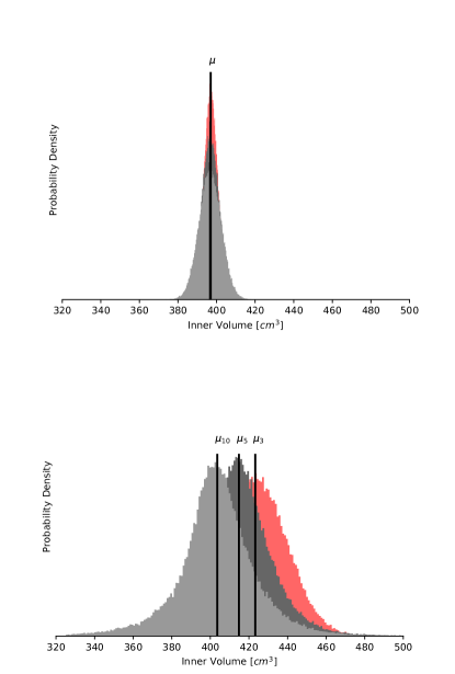
Figure 5. Model B: Probability density functions for the inner volume cavity of the left ventricle assuming two Gaussian random fields as uncertainty in the myofiber architecture: (top) $\sigma_{\rm KL}=0.1$ radians, (bottom) $\sigma_{\rm KL}=0.5$ radians. Colors correspond to different correlation lengths: red ($l=3$ cm), dark gray ($l=5$ cm) and light gray ($l=10$ cm).

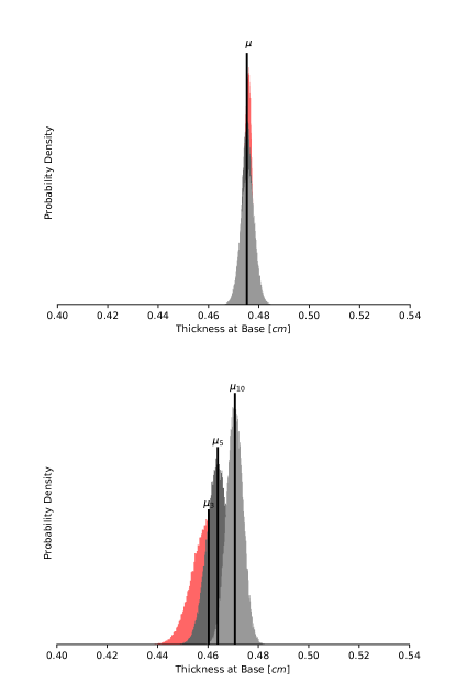
Figure 6. Model B: Probability density functions for the thickness at base assuming two Gaussian random fields as uncertainty in the myofiber architecture: (top) $\sigma_{\rm KL}=0.1$ radians, (bottom) $\sigma_{\rm KL}=0.5$ radians. Colors correspond to different correlation lengths: red ($l=3$ cm), dark gray ($l=5$ cm) and light gray ($l=10$ cm).

Table 4 shows the results of modeling the fiber orientation as a Gaussian random field with a standard deviation of 6 degrees (0.1 radians). We see that all quantities of interest show a constant mean value, independent of the correlation length. The coefficients of variation decreases slightly with decreasing correlation lengths for all quantities of interest except the inner volume, for which its coefficient of variation stays constant at 0.01 across the correlation lengths investigated. Different and more interesting patterns are observed when the standard deviation is increased to 0.5 radians, as shown in Table 5. In this case cavity volume increases from 403 to 424 (cm³) as the correlation length decreases from 10 to 3 (cm). The standard deviation stays approximately constant, and the coefficient of variation is 0.04 for all correlation lengths. Turning now to the apex lengthening, we observe that this is the quantity of interest with the largest coefficient of variation, at $0.07-0.08$ for the correlation lengths examined, with slightly increasing coefficient of variation with increasing correlation length (Table 5). We also observe a slight decrease of the expected value with less correlation in the myofiber variability. Figure 5, shows density distributions for the cavity volume obtained with different perturbation fields. It can be seen that the degree of symmetry remains the same across the correlation lengths compared for both random fields under study. From kurtosis and skewness values (not shown), we confirm that the distributions associated to the inner volume, for both $\sigma_{\rm KL}=0.1$ and 0.5 radians, can be considered as univariate normal distributions (absolute value of both skewness and kurtosis are within the range $\pm 1.96$ [70, 71]). However, in the case of $\sigma_{\rm KL}=0.5$ radians, as the correlation length $l$ increases, the distributions have heavier tails and sharper peak than the normal distribution, while as the correlation of the fiber noise decreases, the diastolic volume results are closer to a Gaussian curve.

From Table 5, we observe that the expected values of both the wall volume and wall thickness decrease with decreasing correlation length, i.e. as the uncertainty in the fiber field approaches a white noise field. The opposite trend holds in terms of the spread or relative uncertainty for these two response quantities; the coefficient of variation increases with increasing correlation length, though always below 3$\%$. These findings are also contrary to the results mentioned above for a narrower width of the perturbation, for which the coefficient of variation diminishes as $l$ decreases. Additionally, the skewness and kurtosis values for those two response quantities are close to zero (absolute value of both moments are within the range $\pm 1.96$ [70, 71]) and thus wall volume and wall thickness distributions fit normal curves, as is also illustrated by Figure 6 for the former quantity. It is interesting to note that in the particular case of correlation length $l=3$ cm and $\sigma_{\rm KL}=0.1$ radians, we observe slightly negatively skewed data, with the left tail of the density distribution being longer and its mass concentrated on the right of the figure.

4. Discussion

The aim of this paper has been to analyze a computational model describing the passive filling phase of the left ventricle using the framework of uncertainty quantification. Our study quantifies the impact of uncertainty in global material parameters, and, more importantly, in measurements of local fiber orientations. The equations governing the passive mechanical behaviour of the heart have been solved using the finite-element software FEniCS [67], and the implemented uncertainty framework is based on polynomial chaos expansions accessible via ChaosPy [68] and truncated Karhunen-Loéve expansions. This non-intrusive method allowed a successful study of the impact of uncertainties, providing statistical analysis through the probability densities of a set of global response model outputs (inner cavity volume, apex lengthening, wall thickening, and wall volume).

In our first simulation model, we identified the main uncertain input parameters and characterized these by random variables obeying certain specific probability distributions. The results clearly point at the multiplicative factor $C$ as the parameter with the largest influence on the variance in model outputs, and $K$, $\alpha_{epi}$, $\beta_{endo}$ and $\beta_{epi}$ as the inputs with the lowest impact on model response uncertainty. Furthermore, the SA results indicate that uncertainty in $C$ may account for up to $75\%$ of the uncertainty in the considered output quantities. Our results suggest that the directional material stiffnesses, both in fiber and cross-fiber directions, contribute less to overall model output variance, but that these parameters are important for wall volume and to some extent wall thickness. On the other hand, our results from model A indicate that randomness in all angle variables, except to some extent the angle at the endocardiac surface ($\alpha_{endo}$), contribute very little to the variance of all output quantities of interest. Thus, even rather rough estimates of these parameters would have little effect on the uncertainty in the output predictions.

These findings may be compared to the results of [29] which also considered the influence of uncertainty in material parameters in the mechanical response of the heart. First, [29] identified the apex lengthening/ventricular elongation as the output quantity most affected by uncertainty in input parameters than the rest of the model outputs compared here. In contrast, our results indicate that the model output with the largest relative uncertainty (largest coefficient of variation) is the variation of the inner cavity volume. Second, a basic sensitivity analysis presented in [29] revealed that the inputs with the largest influence on the uncertainty of the studied response quantities are $b_{xx}$ and $C$. Our results are in partial agreement, as we found that $C$ and $b_{xx}$ are the input parameters with the greatest influence on the output variance only for the inner cavity and the wall volumes. We note that these discrepancies between the present work and previous results may be due to differences in the considered mechanical model and in the applied stochastic sensitivity analysis. In particular, [29] considers an idealized and perfectly symmetric geometrical model, which is likely to substantially impact the results.

Modelling uncertainty in the input parameters for the LDRB algorithm examines only one aspect of the influence of randomness in myocardial fiber architecture. For a more thorough study, we therefore also considered Gaussian perturbation fields of a base LDRB-generated fiber orientation field, thus introducing local perturbations in fiber angle orientation over the computational geometry. Our results reveal that for moderate variability in fiber fields ($\sigma_{\rm KL}=0.1$ radians), the impact on all output quantities of interest is fairly low. The mean values stay constant independent of the correlation length of the field, and the coefficients of variation are small and decrease slightly with decreasing correlation length. For larger field variability ($\sigma_{\rm KL}=0.5$ radians) the influence of the correlation in myofiber uncertainty differs depending on the quantity of interest; for the inner cavity volume the relative uncertainty does not change with the correlation length of the perturbation field, while wall properties, such as thickness or wall volume, experience a larger variation relative to the mean as the correlation length decreases. In contrast, our findings demonstrate the opposite behaviour for the lengthening variation of the left ventricle at apex. Moreover, our results indicate that the variability of the cardiac tissue in terms of fiber arrangement has a greater influence on apex lengthening (coefficient of variation up to 0.08) than any of the parameters considered in model A (coefficient of variation 0.06). This is the only quantity of interest where this is observed. Both for the apex lengthening and inner cavity volume we found non-negligible coefficients of variation for the variability in fiber orientation, independent of the correlation length.

The apparent discrepancies between Model A and Model B have some interesting implications. While most model outputs showed a very low sensitivity to the global input parameters of the LDRB algorithm, the experiment with large local local variations in fiber orientation showed a large impact on the output quantities. These results indicate that as long as a structured, helical arrangements of fiber orientations is maintained, the precise angles of rotation are not that important. On the other hand, any loss of the helical structure, which is seen in Model B for low correlation lengths (Figure 2 right panel), has a substantial impact on the global mechanical properties of the ventricle. In real-world applications, including patient specific simulations, the use of rule-based assignment of fiber orientation will therefore tend to exaggerate tissue organization and thereby the ventricular stiffness. On the other hand, DTMRI based fiber fields capture both true tissue variations and measurement noise, and are likely to underestemate the inherent stiffness of the ventricle.

Future studies may target some of the limitations in this work as discussed here. First, the input parameter uncertainty was modelled using pre-specified normal/log-normal type distributions and independent. For an even more realistic UQ analysis, one should calibrate these probability distributions in accordance with physiological or medical data (if available) via e.g. Bayesian inversion. Second, in order to quantify the variability of the fiber architecture, while we here considered a truncated Karhunen-Loéve expansion, an alternative would be a Principal Component Analysis (PCA). PCA may offer a more realistic quantification of the variability of the fiber perturbation field by its mean and covariance matrix sampled from a cardiac diffusion tensor imaging (DTI) population distribution [28]. Third, other extensions of this study should include not just the filling phase of the heart but also the active contraction of the muscle in the cardiac cycle, as well as taking into account in the same model the uncertainty emerging from both input material parameters and the fiber architecture.

Finally, an important limitation of the present study is that we only consider the propagation of model parameter uncertainty through a forward model of passive cardiac mechanics. In typical applications of cardiac mechanics models, material parameters such as $C,b_{ff},b_{xx},$, and _fx are fitted to match data from patient recordings or experiments. In this context the quantities considered as output variables in the present study become input to a parameter estimation problem [44]. The results obtained in the present study are valuable also in this context, since input variables with high sensitivity indices will be most easily identifiable in an inverse problem setting, while the variables with low sensitivity are essentially non-observable. However, performing a proper UQ of this parameter estimation problem, quantifying how measurement error impact estimated parameters and in turn model predictions, will be a highly relevant extension of the present work.

5. Conclusion

We have performed a detailed UQ and sensitivity analysis of a computational model of passive ventricular mechanics, using a PCE method in combination with a Karhunen-Loéve expansion of stochastic field variables. The methods were verified by comparing selected outputs with results of Quasi-Monte Carlo simulations, confirming that the PCE approach gives an accurate and computationally efficient representation of uncertainty propagation through the cardiac mechanics model. The UQ and sensitivity analysis can be concluded in two main findings. The first is that the the multiplicative factor that scales the strain energy ($C$) is the most sensitive parameter in the material law considered here. The second is that while all considered model outputs are relatively insensitive to the global endo- and epicardial helix angles, they are highly sensitive to local variations and noise in the fiber orientation.

6. Acknowledgments

This research is supported by the Nordic Council of Ministers through Nordforsk grant #74756 (AUQ-PDE), by the Research Council of Norway through FRINATEK grant #250731/F20 (Waterscape) and a Center of Excellence grant to the Center for Biomedical Computing, and by NOTUR grant NN9316K.

References

- [1] Lopez B, Peña E. Patient-Specific Computational Modeling. Lecture Notes in Computational Vision and Biomechanics. Springer Netherlands; 2012.
- [2] Chabiniok R, Wang VY, Hadjicharalambous M, et al. Multiphysics and multiscale modelling, data–model fusion and integration of organ physiology in the clinic: ventricular cardiac mechanics. Interface Focus. 2016;6(2).
- [3] Sack KL, Davies NH, Guccione JM, Franz T. Personalised computational cardiology: Patient-specific modelling in cardiac mechanics and biomaterial injection therapies for myocardial infarction. Heart Fail Rev. 2016;21(6):815–826.
- [4] Zhu Y, Matsumura Y, Wagner WR. Ventricular wall biomaterial injection therapy after myocardial infarction: Advances in material design, mechanistic insight and early clinical experiences. Biomaterials. 2017;129:37–53.
- [5] Biglino G, Capelli C, Bruse J, Bosi GM, Taylor AM, Schievano S. Computational modelling for congenital heart disease: how far are we from clinical translation? Heart. 2017;103(2):98–103.
- [6] Wolters B, Rutten M, Schurink G, Kose U, Hart J, Vosse F. A patient-specific computational model of fluid–structure interaction in abdominal aortic aneurysms. Med Eng Phys. 2005;27(10):871–883.
- [7] Land S, Gurev V, Arens S, et al. Verification of cardiac mechanics software: benchmark problems and solutions for testing active and passive material behaviour. Proc. Mat. Phys. Eng. Sci.. 2015;471(2184).
- [8] Roy CJ, Oberkampf WL. A comprehensive framework for verification, validation, and uncertainty quantification in scientific computing. Comput Methods Appl Mech Engrg. 2011;200(25–28):2131 – 2144.
- [9] Smith RC. Uncertainty Quantification: Theory, Implementation, and Applications. Philadelphia, PA, USA: Society for Industrial and Applied Mathematics; 2013.
- [10] Saltelli A, Ratto M, Andres T, et al. Global Sensitivity Analysis. The Primer. John Wiley & Sons, Ltd; 2008.
- [11] Krishnamurthy A, Villongco CT, Chuang J, et al. Patient-specific models of cardiac biomechanics. J Comput Phys. 2013;244:4 – 21.
- [12] Young AA, Frangi AF. Computational cardiac atlases: from patient to population and back. Exp Physiol. 2009;94(5):578–596.
- [13] Bai W, Shi W, Marvao A, et al. A bi-ventricular cardiac atlas built from 1000+ high resolution MR images of healthy subjects and an analysis of shape and motion. Med Image Anal. 2015;26(1):133–145.
- [14] Wang VY, Lam H, Ennis DB, Cowan BR, Young AA, Nash MP. Modelling passive diastolic mechanics with quantitative {MRI} of cardiac structure and function. Med Image Anal. 2009;13(5):773–784.
- [15] Niederer SA, Plank G, Chinchapatnam P, et al. Length-dependent tension in the failing heart and the efficacy of cardiac resynchronization therapy. Cardiovasc Res. 2011;89(2):336–343.
- [16] Bayer JD, Blake RC, Plank G, Trayanova NA. A novel rule-based algorithm for assigning myocardial fiber orientation to computational heart models. Ann Biomed Eng. 2012;40(10):2243–2254.
- [17] Holzapfel GA, Ogden RW. Constitutive modelling of passive myocardium: a structurally based framework for material characterization. Philos. Trans. A Math Phys. Eng. Sci.. 2009;367(1902):3445–3475.
- [18] Wang HM, Gao H, Luo XY, et al. Structure-based finite strain modelling of the human left ventricle in diastole. J Num Method Biomed Eng. 2013;29(1):83–103.
- [19] Helm P, Beg MF, Miller MI, Winslow RL. Measuring and mapping cardiac fiber and laminar architecture using diffusion tensor mr imaging. Ann New York Acad Sci. 2005;1047(1):296–307.
- [20] Lombaert H, Peyrat J. Human atlas of the cardiac fiber architecture: Study on a healthy population. IEEE Trans Med Imaging. 2012;31(7):1436–1447.
- [21] Toussaint N, Stoeck CT, Schaeffter T, Kozerke S, Sermesant M, Batchelor PG. In vivo human cardiac fibre architecture estimation using shape-based diffusion tensor processing. Med Image Anal. 2013;17(8):1243–1255.
- [22] Nagler A, Bertoglio C, Gee M, Wall W. Personalization of Cardiac Fiber Orientations from Image Data Using the Unscented Kalman Filter:132–140. Springer Berlin Heidelberg 2013.
- [23] Reese TG, Weisskoff RM, Smith RN, Rosen BR, Dinsmore RE, Wedeen VJ. Imaging myocardial fiber architecture in vivo with magnetic resonance. Magn Reson Med. 1995;34(6):786–791.
- [24] Scollan DF, Holmes A, Winslow R, Forder J. Histological validation of myocardial microstructure obtained from diffusion tensor magnetic resonance imaging. American Journal of Physiology - Heart and Circulatory Physiology. 1998;275(6):H2308–H2318.
- [25] Hsu EW, Muzikant AL, Matulevicius SA, Penland RC, Henriquez CS. Magnetic resonance myocardial fiber-orientation mapping with direct histological correlation. Am. J. Physiol. Heart Circ. Physiol. 1998;274(5):H1627–H1634.
- [26] Vadakkumpadan F, Arevalo H, Ceritoglu C, Miller M, Trayanova N. Image-based estimation of ventricular fiber orientations for personalized modeling of cardiac electrophysiology. IEEE Trans Med Imaging. 2012;31(5):1051–1060.
- [27] Geerts L, Kerckhoffs R, Bovendeerd P, Arts T. Towards Patient Specific Models of Cardiac Mechanics: A Sensitivity Study:81–90. Springer Berlin Heidelberg 2003.
- [28] Molléro R, Neumann D, Rohé MM, et al. Propagation of Myocardial Fibre Architecture Uncertainty on Electromechanical Model Parameter Estimation: A Case Study. In: 8th International Conference, FIMH 2015, Maastricht, The Netherlands, June 25-27, 2015. Proceedings:448–456; 2015; Maastricht, Netherlands.
- [29] Osnes H, Sundnes J. Uncertainty analysis of ventricular mechanics using the probabilistic collocation method. IEEE Trans Biomed Eng. 2012;59(8):2171–2179.
- [30] Hurtado DE, Castro S, Madrid P. Uncertainty quantification of 2 models of cardiac electromechanics. J Num Method Biomed Eng. 2017;33(12):e2894–n/a.
- [31] Pluijmert M, Delhaas T, Parra AF, Kroon W, Prinzen FW, Bovendeerd PHM. Determinants of biventricular cardiac function: a mathematical model study on geometry and myofiber orientation. Biomech Model Mechanobiol. 2017;16(2):721–729.
- [32] Hassaballah A, Hassan M, Mardi A, Hamdi M. Modeling the effects of myocardial fiber architecture and material properties on the left ventricle mechanics during rapid filling phase. Appl. Math. Infor. Sci.. 2015;9:161–167.
- [33] Nikou A, Gorman RC, Wenk JF. Sensitivity of left ventricular mechanics to myofiber architecture: A finite element study. Proceedings of the Institution of Mechanical Engineers, Part H: Journal of Engineering in Medicine. 2016;230(6):594–598.
- [34] Wang X. Variance reduction techniques and quasi-Monte Carlo methods. J Comput Appl Math. 2001;132(2):309 – 318.
- [35] Rubinstein RY, Kroese DP. Simulation and the Monte Carlo Method. Wiley-Interscience; 2007.
- [36] Giles MB. Multilevel Monte Carlo methods. Acta Numer. 2015;24:259–328.
- [37] Sudret B, Marelli S, Wiart J. Surrogate models for uncertainty quantification: An overview. In: 11th European Conference on Antennas and Propagation (EUCAP):793–797; 2017.
- [38] Wiener N. The homogeneous chaos. Amer J Math. 1938;60(4):897–936.
- [39] Yang S, Xiong F, Wang F. Polynomial Chaos Expansion for Probabilistic Uncertainty Propagation. Rijeka: InTech; 2017.
- [40] Swenson DJ, Geneser SE, Stinstra JG, Kirby RM, MacLeod RS. Cardiac position sensitivity study in the electrocardiographic forward problem using stochastic collocation and boundary element methods. Ann Biomed Eng. 2011;39(12):2900–2910.
- [41] Loéve M. Fundamental limit theorems of probability theory. Ann. Math. Statist.. 1950;21(3):321–338.
- [42] Guccione JM, Costa KD, McCulloch AD. Finite element stress analysis of left ventricular mechanics in the beating dog heart. J Biomech. 1995;28(10):1167 – 1177.
- [43] Streeter DD, Spotnitz HM, Patel DP, Ross J, Sonnenblick EH. Fiber orientation in the canine left ventricle during diastole and systole. Circ Res. 1969;24(3):339–347.
- [44] Balaban G, Finsberg H, Odland HH, et al. High-resolution data assimilation of cardiac mechanics applied to a dyssynchronous ventricle. J Num Method Biomed Eng. 2017;33(11):e2863–n/a.
- [45] Xiu D. Numerical Methods for Stochastic Computations: A Spectral Method Approach. Princeton University Press; 2010.
- [46] Tatang MA, Pan W, Prinn RG, McRae GJ. An efficient method for parametric uncertainty analysis of numerical geophysical models. J. Geophys. Res. D. 1997;102(D18):21925–21932.
- [47] Hosder S, Walters RW, Balch M. Efficient sampling for non-intrusive polynomial chaos applications with multiple uncertain input variables. In: 48th AIAA/ASME/ASCE/AHS/ASC Structures, Structural Dynamics, and Materials Conference, vol. 125: ; 2007; Honolulu, Hawaii.
- [48] Dick J, Kuo FY, Sloan IH. High-dimensional integration: The quasi-Monte Carlo way. Acta Numer. 2013;22:133–288.
- [49] Kendall MGMG. The advanced theory of statistics. New York, Hafner; 1958.
- [50] Halton JH. On the efficiency of certain quasi-random sequences of points in evaluating multi-dimensional integrals. Numer Math. 1960;2(1):84–90.
- [51] Saltelli A. Making best use of model evaluations to compute sensitivity indices. Comput Phys Comm. 2002;145(2):280 – 297.
- [52] Iooss B, Lemaître P. A Review on Global Sensitivity Analysis Methods:101–122. Boston, MA: Springer US 2015.
- [53] Sobol I. Global sensitivity indices for nonlinear mathematical models and their Monte Carlo estimates. Math Comput Simulation. 2001;55(1-3):271 – 280.
- [54] Eck VG, Donders WP, Sturdy J, et al. A guide to uncertainty quantification and sensitivity analysis for cardiovascular applications. J Num Method Biomed Eng. 2016;32(8):e02755–n/a.
- [55] Roger G. Ghanem PS. Stochastic Finite Elements: A Spectral Approach. Springer-Verlag New York; 1991.
- [56] Rasmussen CE, Williams CKI. Gaussian Processes for Machine Learning (Adaptive Computation and Machine Learning). The MIT Press; 2005.
- [57] Betz W, Papaioannou I, Straub D. Numerical methods for the discretization of random fields by means of the Karhunen–Loéve expansion. Comput Methods Appl Mech Engrg. 2014;271(Supplement C):109 – 129.
- [58] Atkinson K. The Numerical Solution of Integral Equations of the Second Kind. Cambridge University Press; 1997.
- [59] Hackbusch W. Integral Equations: Theory and Numerical Treatment. International Series of Numerical Mathematics. Birkhäuser Basel; 1995.
- [60] Khoromskij BN, Litvinenko A, Matthies HG. Application of hierarchical matrices for computing the Karhunen–Loève expansion. Computing. 2009;84(1):49–67.
- [61] Saibaba AK, Lee J, Kitanidis PK. Randomized algorithms for generalized hermitian eigenvalue problems with application to computing Karhunen–Loéve expansion. Numer Linear Algebra Appl. 2016;23(2):314–339.
- [62] Grasedyck L, Hackbusch W. Construction and arithmetics of H-matrices. Computing. 2003;70(4):295–334.
- [63] Hackbusch W, Khoromskij BN. A sparse H-matrix arithmetic. Part II: Application to multidimensional problems. Computing. 2000;64(1):21–47.
- [64] Hackbusch W. A sparse matrix arithmetic based on H-matrices. Part I: Introduction to H-matrices. Computing. 1999;62(2):89–108.
- [65] Bebendorf M, Rjasanow S. Adaptive low-rank approximation of collocation matrices. Computing. 2003;70(1):1–24.
- [66] Alnæs MS, Blechta J, Hake J, et al. The FEniCS Project Version 1.5. Archive of Numerical Software. 2015;3(100):9–23.
- [67] Logg A, Ølgaard KB, Rognes ME, Wells GN. FFC: the FEniCS Form Compiler. ch. 11. Springer 2012.
- [68] Feinberg J, Langtangen HP. Chaospy: An open source tool for designing methods of uncertainty quantification. J. Comput. Sci.. 2015;11:46 - 57.
- [69] Jones E, Oliphant T, Peterson P. SciPy: Open source scientific tools for Python. 2001.
- [70] Gravetter F, Wallnau L. Essentials of Statistics for the Behavioral Sciences. Boston, MA (USA): Cengage Learning; 2013.
- [71] Trochim W, Donnelly J. The Research Methods Knowledge Base. Boston, MA (USA): Cengage Learning; 2006.