Multiplexing Analysis of Millimeter-Wave Massive MIMO Systems

Abstract

This paper is concerned with spatial multiplexing analysis for millimeter-wave (mmWave) massive MIMO systems. For a single-user mmWave system employing distributed antenna subarray architecture in which the transmitter and receiver consist of $K_{t}$ and $K_{r}$ subarrays, respectively, an asymptotic multiplexing gain formula is firstly derived when the numbers of antennas at subarrays go to infinity. Specifically, assuming that all subchannels have the same average number of propagation paths $\bar{L}$, the formula implies that by employing such a distributed antenna-subarray architecture, an exact average maximum multiplexing gain of $K_{r}K_{t}\bar{L}$ can be achieved. This result means that compared to the co-located antenna architecture, using the distributed antenna-subarray architecture can statistically scale up the maximum multiplexing gain proportionally to $K_{r}K_{t}$. In order to further reveal the relation between diversity gain and multiplexing gain, a simple characterization of the diversity-multiplexing tradeoff is also given. The multiplexing gain analysis is then extended to the multiuser scenario as well as the conventional partially-connected RF structure in the literature. Moreover, simulation results obtained with the hybrid analog/digital processing corroborate the analysis results.

I Introduction

Recently, millimeter-wave (mmWave) communication has gained considerable attention as a candidate technology for 5G mobile communication systems and beyond [1, 2, 3]. The main reason for this is the availability of vast spectrum in the mmWave band (typically 30-300 GHz) that is very attractive for high data rate communications. However, compared to communication systems operating at lower microwave frequencies (such as those currently used for 4G mobile communications), propagation loss in mmWave frequencies is much higher, in the orders-of-magnitude. Fortunately, given the much smaller carrier wavelengths, mmWave communication systems can make use of compact massive antenna arrays to compensate for the increased propagation loss.

Nevertheless, the large-scale antenna arrays together with high cost and large power consumption of the mixed analog/digital signal components makes it difficult to equip a separate radio-frequency (RF) chain for each antenna and perform all the signal processing in the baseband. Therefore, research on hybrid analog-digital processing of precoder and combiner for mmWave communication systems has attracted very strong interests from both academia and industry [4]$\;-$[16]. In particular, a lot of work has been performed to address challenges in using a limited number of RF chains. For example, the authors in [4] considered single-user precoding in mmWave massive MIMO systems and established the optimality of beam steering for both single-stream and multi-stream transmission scenarios. In [10], the authors showed that hybrid processing can realize any fully digital processing if the number of RF chains is twice the number of data streams. However, due to the fact that mmWave signal propagation has an important feature of multipath sparsity in both the temporal and spatial domains [17, 18, 19, 20], it is expected that the potentially available benefits of diversity and multiplexing are indeed not large if the deployment of the antenna arrays is co-located. In order to enlarge diversity/multiplexing gains in mmWave massive MIMO communication systems, this paper consider the use of a more general array architecture, called distributed antenna subarray architecture, which includes lo-located array architecture as a special case. It is pointed out that distributed antenna systems have received strong interest as a promising technique to satisfy such growing demands for future wireless communication networks due to the increased spectral efficiency and expanded coverage [21]$\;-$[25].

It is well known that diversity-multiplexing tradeoff (DMT) is a compact and convenient framework to compare different MIMO systems in terms of the two main and related system indicators: data rate and error performance [26, 27, 28, 29, 30, 31]. This tradeoff was originally characterized by Zheng and Tse [26] for MIMO communication systems operating over independent and identically distributed (i.i.d.) Rayleigh fading channels. The framework has then ignited a lot of interests in analyzing various communication systems and under different channel models. For a mmWave massive MIMO system, how to quantify the diversity and multiplexing performance and further characterize its DMT is a fundamental and open research problem. In particular, to the best of our knowledge, until now there is no unified multiplexing gain analysis for mmWave massive MIMO systems that is applicable to both co-located and distributed antenna array architectures.

To fill this gap, this paper investigates the multiplexing performance of mmWave massive MIMO systems with the proposed distributed subarray architecture. The focus is on the asymptotical multiplexing gain analysis in order to find out the potential multiplexing advantage provided by multiple distributed antenna arrays. The obtained analysis can be used conveniently to compare various mmWave massive MIMO systems with different distributed antenna array structures.

The main contributions of this paper are summarized as follows:

• For a single-user system with the proposed distributed subarray architecture, a multiplexing gain expression is obtained when the number of antennas at each subarray increases without bound. This expression clearly indicates that one can obtain a large multiplexing gain by employing the distributed subarray architecture.

• A simple DMT characterization is further given. It can reveal the relation between diversity gain and multiplexing gain and let us obtain insights to understand the overall resources provided by the distributed antenna architecture.

• The multiplexing gain analysis is then extended to the multiuser scenario with downlink and uplink transmission, as well as the single-user system employing the conventional partially-connected RF structure based distributed subarrays.

• Simulation results are provided to corroborate the analysis results and show that the distributed subarray architecture yields significantly better multiplexing performance than the co-located single-array architecture.

The remainder of this paper is organized as follows. Section II describes the massive MIMO system model and hybrid processing with the distributed subarray architecture in mmWave fading channels. Section III and Section IV provides the asymptotical achievable rate analysis and the multiplexing gain analysis for the single-user mmWave system, respectively. In Section V and VI, the multiplexing gain analysis is extended to the scenario with the partially-connected RF architecture and the multiuser scenario, respectively. Section VII concludes the paper.

Throughout this paper, the following notations are used. Boldface upper and lower case letters denote matrices and column vectors, respectively. The superscripts $(\cdot)^{T}$ and $(\cdot)^{H}$ stand for transpose and conjugate-transpose, respectively. $\mathrm{diag}\{a_{1},a_{2},\ldots,a_{N}\}$ stands for a diagonal matrix with diagonal elements $\{a_{1},a_{2},\ldots,a_{N}\}$. The expectation operator is denoted by $\mathbb{E}(\cdot)$. $[\mathbf{A}]_{ij}$ gives the $(i,j)$th entry of matrix $\mathbf{A}$. $\mathbf{A}\bigotimes\mathbf{B}$ is the Kronecker product of $\mathbf{A}$ and $\mathbf{B}$. We write a function $a(x)$ of $x$ as $o(x)$ if $\lim_{x\to 0}a(x)/x=0$. We use $(x)^{+}$ to denote $\max\{0,x\}$. Finally, $\mathcal{CN}(0,1)$ denotes a circularly symmetric complex Gaussian random variable with zero mean and unit variance.

II System Model

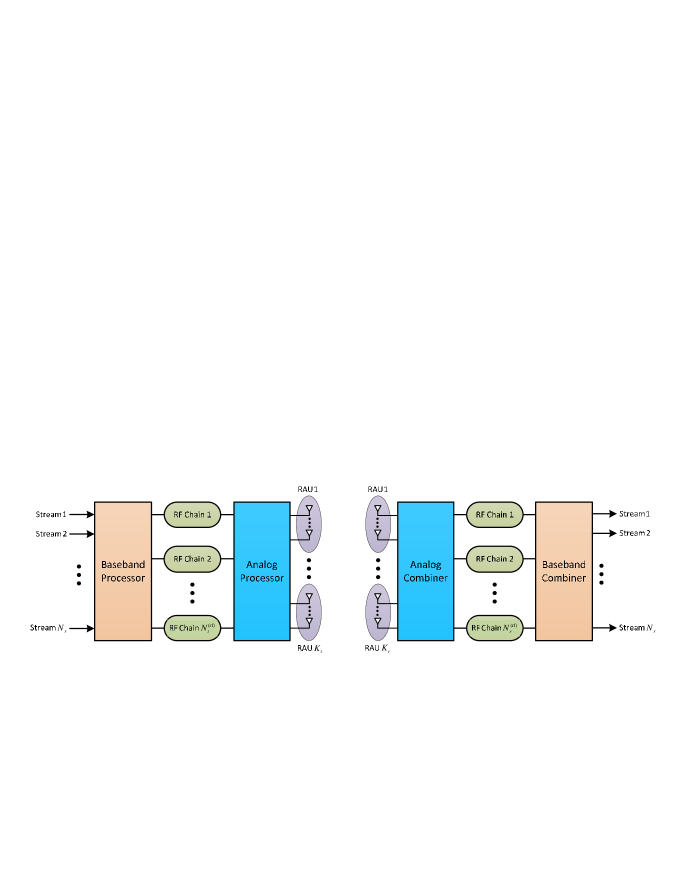
Figure 1: Block diagram of a mmWave massive MIMO system with distributed antenna arrays.

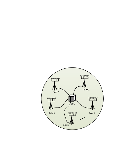
Figure 2: Illustration of distributed antenna array deployment.

Consider a single-user mmWave massive MIMO system as shown in Fig. 1. The transmitter is equipped with a distributed antenna array to send $N_{s}$ data streams to a receiver, which is also equipped with a distributed antenna array. Here, a distributed antenna array means an array consisting of several remote antenna units (RAUs) (i.e., antenna subarrays) that are distributively located, as depicted in Fig. 2. Specifically, the antenna array at the transmitter consists of $K_{t}$ RAUs, each of which has $N_{t}$ antennas and is connected to a baseband processing unit (BPU) by fiber. Likewise, the distributed antenna array at the receiver consists of $K_{r}$ RAUs, each having $N_{r}$ antennas and also being connected to a BPU by fibers. Such a MIMO system shall be referred to as a $(K_{t},N_{t},K_{r},N_{r})$ distributed MIMO (D-MIMO) system. When $K_{t}=K_{r}=1$, the system reduces to a conventional co-located MIMO (C-MIMO) system.

The transmitter accepts as its input $N_{s}$ data streams and is equipped with $N_{t}^{({\rm rf})}$ RF chains, where $N_{s}\leq N_{t}^{({\rm rf})}\leq N_{t}K_{t}$. Given $N_{t}^{({\rm rf})}$ transmit RF chains, the transmitter can apply a low-dimension $N_{t}^{({\rm rf})}\times N_{s}$ baseband precoder, $\mathbf{W}_{t}$, followed by a high-dimension $K_{t}N_{t}\times N_{t}^{({\rm rf})}$ RF precoder, $\mathbf{F}_{t}$. Note that amplitude and phase modifications are feasible for the baseband precoder $\mathbf{W}_{t}$, while only phase changes can be made by the RF precoder $\mathbf{F}_{t}$ through the use of variable phase shifters and combiners. The transmitted signal vector can be written as

$$\mathbf{x}=\mathbf{F}_{t}\mathbf{W}_{t}\mathbf{P}_{t}^{1/2}\mathbf{s},$$ (1)

where $\mathbf{s}$ is the $N_{s}\times 1$ symbol vector such that $\mathbb{E}[\mathbf{s}\mathbf{s}^{H}]=\mathbf{I}_{N_{s}}$, and $\mathbf{P}_{t}=[p_{ij}]$ is a diagonal power allocation matrix with $\sum_{l=1}^{N_{s}}p_{ll}=P$. Thus $P$ represents the average total input power. Considering a narrowband block fading channel, the $K_{r}N_{r}\times 1$ received signal vector is

$$\mathbf{y}=\mathbf{H}\mathbf{F}_{t}\mathbf{W}_{t}\mathbf{P}_{t}^{1/2}\mathbf{s}+\mathbf{n}$$ (2)

where $\mathbf{H}$ is $K_{r}N_{r}\times K_{t}N_{t}$ channel matrix and $\mathbf{n}$ is a $K_{r}N_{r}\times 1$ vector consisting of i.i.d. $\mathcal{CN}(0,1)$ noise samples. Throughout this paper, $\mathbf{H}$ is assumed known to both the transmitter and receiver. Given that $N_{r}^{({\rm rf})}$ RF chains (where $N_{s}\leq N_{r}^{({\rm rf})}\leq N_{r}K_{r}$) are used at the receiver to detect the $N_{s}$ data streams, the processed signal is given by

$$\mathbf{z}=\mathbf{W}_{r}^{H}\mathbf{F}_{r}^{H}\mathbf{H}\mathbf{F}_{t}\mathbf{W}_{t}\mathbf{P}_{t}^{1/2}\mathbf{s}+\mathbf{W}_{r}^{H}\mathbf{F}_{r}^{H}\mathbf{n}$$ (3)

where $\mathbf{F}_{r}$ is the $K_{r}N_{r}\times N_{r}^{({\rm rf})}$ RF combining matrix, and $\mathbf{W}_{r}$ is the $N_{r}^{({\rm rf})}\times N_{s}$ baseband combining matrix. When Gaussian symbols are transmitted over the mmWave channel, the the system achievable rate is expressed as

$$R=\log_{2}|\mathbf{I}_{N_{s}}+\mathbf{R}_{n}^{-1}\mathbf{W}_{r}^{H}\mathbf{F}_{r}^{H}\mathbf{H}\mathbf{F}_{t}\mathbf{W}_{t}\mathbf{P}_{t}\mathbf{W}_{t}^{H}\mathbf{F}_{t}^{H}\mathbf{H}^{H}\mathbf{F}_{r}\mathbf{W}_{r}|$$ (4)

where $\mathbf{R}_{n}=\mathbf{W}_{r}^{H}\mathbf{F}_{r}^{H}\mathbf{F}_{r}\mathbf{W}_{r}$.

Furthermore, according to the architecture of RAUs at the transmitting and receiving ends, $\mathbf{H}$ can be written as

$$\mathbf{H}=\left[\begin{array}[]{lll}\sqrt{g_{11}}\mathbf{H}_{11}&\cdots&\;\;\sqrt{g_{1K_{t}}}\mathbf{H}_{1K_{t}}\\ \;\;\;\;\vdots&\ddots&\;\;\;\;\;\;\;\;\vdots\\ \sqrt{g_{K_{r}1}}\mathbf{H}_{K_{r}1}&\cdots&\sqrt{g_{K_{r}K_{t}}}\mathbf{H}_{K_{r}K_{t}}\end{array}\right].$$ (5)

In the above expression, $g_{ij}$ represents the large scale fading effect between the $i$th RAU at the receiver and the $j$th RAU at the transmitter, which is assumed to be constant over many coherence-time intervals. The normalized subchannel matrix $\mathbf{H}_{ij}$ represents the MIMO channel between the $j$th RAU at the transmitter and the $i$th RAU at the receiver. We assume that all of $\{\mathbf{H}_{ij}\}$ are independent mutually each other.

A clustered channel model based on the extended Saleh-Valenzuela model is often used in mmWave channel modeling and standardization [4] and it is also adopted in this paper. For simplicity of exposition, each scattering cluster is assumed to contribute a single propagation path. Using this model, the subchannel matrix $\mathbf{H}_{ij}$ is given by

$$\mathbf{H}_{ij}=\sqrt{\frac{N_{t}N_{r}}{L_{ij}}}\sum_{l=1}^{L_{ij}}\alpha_{ij}^{l}\mathbf{a}_{r}(\phi^{rl}_{ij},\theta^{rl}_{ij})\mathbf{a}_{t}(\phi^{tl}_{ij},\theta^{tl}_{ij})^{H},$$ (6)

where $L_{ij}$ is the number of propagation paths, $\alpha_{ij}^{l}$ is the complex gain of the $l$th ray, and $\phi^{rl}_{ij}$ ($\theta^{rl}_{ij}$) and $\phi^{tl}_{ij}$ ($\theta^{tl}_{ij}$) are its random azimuth (elevation) angles of arrival and departure, respectively. Without loss of generality, the complex gains $\alpha_{ij}^{l}$ are assumed to be $\mathcal{CN}(0,1)$. The vectors $\mathbf{a}_{r}(\phi^{rl}_{ij},\theta^{rl}_{ij})$ and $\mathbf{a}_{t}(\phi^{tl}_{ij},\theta^{tl}_{ij})$ are the normalized receive/transmit array response vectors at the corresponding angles of arrival/departure. For an $N$-element uniform linear array (ULA) , the array response vector is

$$\mathbf{a}^{\mathrm{ULA}}(\phi)=\frac{1}{\sqrt{N}}\left[1,{\mathrm{e}}^{j2\pi\frac{d_{u}}{\lambda}\sin(\phi)},\ldots,{\mathrm{e}}^{j2\pi(N-1)\frac{d_{u}}{\lambda}\sin(\phi)}\right]^{T}$$ (7)

where $\lambda$ is the wavelength of the carrier and $d_{u}$ is the inter-element spacing. It is pointed out that the angle $\theta$ is not included in the argument of $\mathbf{a}^{\mathrm{ULA}}$ since the response for an ULA is independent of the elevation angle. In contrast, for a uniform planar array (UPA), which is composed of $N_{h}$ and $N_{v}$ antenna elements in the horizontal and vertical directions, respectively, the array response vector is represented by

$$\mathbf{a}^{\mathrm{UPA}}(\phi,\theta)=\mathbf{a}^{\mathrm{ULA}}_{h}(\phi)\otimes\mathbf{a}^{\mathrm{ULA}}_{v}(\theta),$$ (8)

where

$$\mathbf{a}^{\mathrm{ULA}}_{h}(\phi)=\frac{1}{\sqrt{N_{h}}}\left[1,{\mathrm{e}}^{j2\pi\frac{d_{h}}{\lambda}\sin(\phi)},\ldots,{\mathrm{e}}^{j2\pi(N_{h}-1)\frac{d_{h}}{\lambda}\sin(\phi)}\right]^{T}$$ (9)

and

$$\mathbf{a}^{\mathrm{ULA}}_{v}(\theta)=\frac{1}{\sqrt{N_{v}}}\left[1,{\mathrm{e}}^{j2\pi\frac{d_{v}}{\lambda}\sin(\theta)},\ldots,{\mathrm{e}}^{j2\pi(N^{v}-1)\frac{d_{v}}{\lambda}\sin(\theta)}\right]^{T}.$$ (10)

III Asymptotic Achievable Rate Analysis

From the structure and definition of the channel matrix $\mathbf{H}$ in Section II, there is a total of $L_{s}=\sum_{i=1}^{K_{r}}\sum_{j=1}^{K_{t}}L_{ij}$ propagation paths. Naturally, $\mathbf{H}$ can be decomposed into a sum of $L_{s}$ rank-one matrices, each corresponding to one propagation path. Specifically, $\mathbf{H}$ can be rewritten as

$$\mathbf{H}=\sum_{i=1}^{K_{r}}\sum_{j=1}^{K_{t}}\sum_{l=1}^{L_{ij}}\tilde{\alpha}_{ij}^{l}\tilde{\mathbf{a}}_{r}(\phi^{rl}_{ij},\theta^{rl}_{ij})\tilde{\mathbf{a}}_{t}^{H}(\phi^{tl}_{ij},\theta^{tl}_{ij}),$$ (11)

where

$$\tilde{\alpha}_{ij}^{l}=\sqrt{g_{ij}\frac{N_{t}N_{r}}{L_{ij}}}\alpha_{ij}^{l},$$ (12)

$\tilde{\mathbf{a}}_{r}(\phi^{rl}_{ij},\theta^{rl}_{ij})$ is a $K_{r}N_{r}\times 1$ vector whose $b$th entry is defined as

$$[\tilde{\mathbf{a}}_{r}(\phi^{rl}_{ij},\theta^{rl}_{ij})]_{b}=\left\{\begin{array}[]{ll}[\mathbf{a}_{r}(\phi^{rl}_{ij},\theta^{rl}_{ij})]_{b-(i-1)N_{r}},&b\in Q_{i}^{r}\\ 0,&b\notin Q_{i}^{r}\end{array}\right.$$ (13)

where $Q_{i}^{r}=((i-1)N_{r},iN_{r}]$. And $\tilde{\mathbf{a}}_{t}(\phi^{tl}_{ij},\theta^{tl}_{ij})$ is a $K_{t}N_{t}\times 1$ vector whose $b$th entry is defined as

$$[\tilde{\mathbf{a}}_{t}(\phi^{tl}_{ij},\theta^{tl}_{ij})]_{b}=\left\{\begin{array}[]{ll}[\mathbf{a}_{t}(\phi^{tl}_{ij},\theta^{tl}_{ij})]_{b-(j-1)N_{t}},&b\in Q_{j}^{t}\\ 0,&b\notin Q_{j}^{t}.\end{array}\right.$$ (14)

where $Q_{j}^{t}=((j-1)N_{t},jN_{t}]$. Regarding $\{\tilde{\mathbf{a}}_{r}(\phi^{rl}_{ij},\theta^{rl}_{ij})\}$ and $\{\tilde{\mathbf{a}}_{t}(\phi^{tl}_{ij},\theta^{tl}_{ij})\}$, we have the following lemma from [32].

Lemma 1

Suppose that the antenna configurations at all RAUs are either ULA or UPA. Then all $L_{s}$ vectors $\{\tilde{\mathbf{a}}_{r}(\phi^{rl}_{ij},\theta^{rl}_{ij})\}$ are orthogonal to each other when $N_{r}\to\infty$. Likewise, all $L_{s}$ vectors $\{\tilde{\mathbf{a}}_{t}(\phi^{tl}_{ij},\theta^{tl}_{ij})\}$ are orthogonal to each other when $N_{t}\to\infty$.

Mathematically, the distributed massive MIMO system can be considered as a co-located massive MIMO system with $L_{s}$ paths that have complex gains $\{\tilde{\alpha}_{ij}^{l}\}$, receive array response vectors $\{\tilde{\mathbf{a}}_{r}(\phi^{rl}_{ij},\theta^{rl}_{ij})\}$ and transmit response vectors $\{\tilde{\mathbf{a}}_{t}(\phi^{tl}_{ij},\theta^{tl}_{ij})\}$. Furthermore, order all paths in a decreasing order of the absolute values of the complex gains $\{\tilde{\alpha}_{ij}^{l}\}$. Then the channel matrix can be written as

$$\mathbf{H}=\sum_{l=1}^{L_{s}}\tilde{\alpha}^{l}\tilde{\mathbf{a}}_{r}(\phi^{rl},\theta^{rl})\tilde{\mathbf{a}}_{t}(\phi^{tl},\theta^{tl})^{H},$$ (15)

where $\tilde{\alpha}^{1}\geq\tilde{\alpha}^{2}\geq\cdots\geq\tilde{\alpha}^{L_{s}}$.

One can rewrite $\mathbf{H}$ in a matrix form as

$$\mathbf{H}=\mathbf{A}_{r}\mathbf{D}\mathbf{A}_{t}^{H}$$ (16)

where $\mathbf{D}$ is a $L_{s}\times L_{s}$ diagonal matrix with $[\mathbf{D}]_{ll}=\tilde{\alpha}^{l}$, and $\mathbf{A}_{r}$ and $\mathbf{A}_{t}$ are defined as follows:

$$\mathbf{A}_{r}=[\tilde{\mathbf{a}}_{r}(\phi^{r1},\theta^{r1}),\ldots,\tilde{\mathbf{a}}_{r}(\phi^{rL_{s}},\theta^{rL_{s}})]$$ (17)

and

$$\mathbf{A}_{t}=[\tilde{\mathbf{a}}_{t}(\phi^{t1},\theta^{t1}),\ldots,\tilde{\mathbf{a}}_{t}(\phi^{tL_{s}},\theta^{tL_{s}})].$$ (18)

Since both $\{\tilde{\mathbf{a}}_{r}(\phi^{rl},\theta^{rl})\}$ and $\{\tilde{\mathbf{a}}_{t}(\phi^{tl},\theta^{tl})\}$ are orthogonal vector sets when $N_{r}\to\infty$ and $N_{t}\to\infty$, $\mathbf{A}_{r}$ and $\mathbf{A}_{t}$ are asymptotically unitary matrices. Then one can form a singular value decomposition (SVD) of matrix $\mathbf{H}$ as

$$\mathbf{H}=\mathbf{U}\mathbf{\Sigma}\mathbf{V}^{H}=[\mathbf{A}_{r}|\mathbf{A}_{r}^{\bot}]\mathbf{\Sigma}[\tilde{\mathbf{A}}_{t}|\tilde{\mathbf{A}}_{t}^{\bot}]^{H}$$ (19)

where $\mathbf{\Sigma}$ is a diagonal matrix containing all singular values on its diagonal, i.e.,

$$[\mathbf{\Sigma}]_{ll}=\left\{\begin{array}[]{ll}|\tilde{\alpha}^{l}|,&\mbox{for}\;1\leq l\leq L_{s}\\ 0,&\mbox{for}\;l>L_{s}\end{array}\right.$$ (20)

and the submatrix $\tilde{\mathbf{A}}_{t}$ is defined as

$$\tilde{\mathbf{A}}_{t}=[{\mathrm{e}}^{j\psi_{1}}\tilde{\mathbf{a}}_{t}(\phi^{t1},\theta^{t1}),\ldots,{\mathrm{e}}^{j\psi_{L_{s}}}\tilde{\mathbf{a}}_{t}(\phi^{tL_{s}},\theta^{tL_{s}})]$$ (21)

where $\psi_{l}$ is the phase of complex gain $\tilde{\alpha}^{l}$ corresponding to the $l$th path. Based on (19), the optimal precoder and combiner are chosen, respectively, as

$$[\mathbf{F}_{t}\mathbf{W}_{t}]_{\mathrm{opt}}=[{\mathrm{e}}^{j\psi_{1}}\tilde{\mathbf{a}}_{t}(\phi^{t1},\theta^{t1}),\ldots,{\mathrm{e}}^{j\psi_{L_{s}}}\tilde{\mathbf{a}}_{t}(\phi^{tN_{s}},\theta^{tN_{s}})]$$ (22)

and

$$[\mathbf{F}_{r}\mathbf{W}_{r}]_{\mathrm{opt}}=[\tilde{\mathbf{a}}_{r}(\phi^{r1},\theta^{r1}),\ldots,\tilde{\mathbf{a}}_{r}(\phi^{rN_{s}},\theta^{rN_{s}})].$$ (23)

To summarize, when $N_{t}$ and $N_{r}$ are large enough, the massive MIMO system can employ the optimal precoder and combiner given in (22) and (23), respectively.

For a given $l$, there are $l^{\prime}$, $i^{\prime}$ and $j^{\prime}$ such that $\tilde{\alpha}^{l}=\tilde{\alpha}_{i^{\prime}j^{\prime}}^{l^{\prime}}=\sqrt{g_{i^{\prime}j^{\prime}}\frac{N_{t}N_{r}}{L_{i^{\prime}j^{\prime}}}}\alpha_{i^{\prime}j^{\prime}}^{l^{\prime}}$. So we introduce two notations:

$$\tilde{\gamma}_{l}=p_{ll}g_{i^{\prime}j^{\prime}}\frac{N_{t}N_{r}}{L_{i^{\prime}j^{\prime}}}$$ (24)

and

$$\tilde{\beta}_{l}=\alpha_{i^{\prime}j^{\prime}}^{l^{\prime}}.$$ (25)

Then it follows from the above SVD analysis that the instantaneous SNR of the $l$th data stream is given by

$$\mathrm{SNR}_{l}=p_{ll}|\tilde{\alpha}^{l}|^{2}=\tilde{\gamma}_{l}|\tilde{\beta}_{l}|^{2},\;\;l=1,2,\ldots,N_{s}.$$ (26)

So we obtain another lemma.

Lemma 2

Suppose that both sets $\{\tilde{\mathbf{a}}_{r}(\phi^{rl}_{ij},\theta^{rl}_{ij})\}$ and $\{\tilde{\mathbf{a}}_{t}(\phi^{tl}_{ij},\theta^{tl}_{ij})\}$ are orthogonal vector sets when $N_{r}\to\infty$ and $N_{t}\to\infty$. Let $N_{s}\leq L_{s}$. In the limit of large $N_{t}$ and $N_{r}$, then the system achievable rate is given by

$$R=\sum_{l=1}^{Ns}\log_{2}(1+\tilde{\gamma}_{l}|\tilde{\beta}_{l}|^{2}).$$ (27)

Remark 1: (22) and (23) indicate that when $N_{t}$ and $N_{r}$ is large enough, the optimal precoder and combiner can be implemented fully in RF using phase shifters [4]. Furthermore, (13) and (14) imply that for each data stream only a couple of RAUs needs the operation of phase shifters at each channel realization.

Remark 2: By using the optimal power allocation (i.e., the well-known waterfilling power allocation [33]), the system can achieve a maximum achievable rate, which is denoted as $R_{o}$. We use $R_{e}(P/N_{s})$ to denote the achievable rate obtained by using the equal power allocation, namely, $p_{ll}=\frac{P}{N_{s}},\;l=1,2,\ldots,N_{s}.$ Then

$$R_{e}(P/N_{s})\leq R_{o}\leq R_{e}((PN_{s})/N_{s})=R_{e}(P).$$ (28)

By doing expectation operation on (28), (28) becomes,

$$\bar{R}_{e}(P/N_{s})\leq\bar{R}_{o}\leq\bar{R}_{e}(P).$$ (29)

In what follows, we derive an asymptotic expression of the ergodic achievable rate with the equal power allocation, $\bar{R}_{e}(P/N_{s})$ (or $\bar{R}_{e}$ for simplicity). For this reason, we need to define an integral function

$$\Delta(x) = \int_{0}^{+\infty}\log_{2}(1+t)e^{-t/x}\frac{1}{x}dt$$ (30)

$$= \log_{2}(e)e^{1/x}E_{1}(1/x)$$

where $E_{1}(\cdot)$ is the exponential integral of a first-order function defined as [34], [35]

$$E_{1}(y) = \int_{1}^{+\infty}\frac{e^{-yt}}{t}dt$$ (31)

$$= -E+\ln(y)-\sum_{k=1}^{\infty}\frac{(-y)^{k}}{k\cdot k!}$$

with $E$ being the Euler constant.

Theorem 1

Suppose that both sets $\{\tilde{\mathbf{a}}_{r}(\phi^{rl}_{ij},\theta^{rl}_{ij})\}$ and $\{\tilde{\mathbf{a}}_{t}(\phi^{tl}_{ij},\theta^{tl}_{ij})\}$ are orthogonnal vector sets when $N_{r}\to\infty$ and $N_{t}\to\infty$. Let $N_{s}\leq L_{s}$ and $\tilde{\gamma}_{1}=\tilde{\gamma}_{2}=\ldots=\tilde{\gamma}_{L_{s}}=\tilde{\gamma}$. Then in the limit of large $N_{t}$ and $N_{r}$, the ergodic achievable rate with homogeneous coefficient set $\{\tilde{\gamma}_{l}\}$, denoted $\bar{R}_{eh}$, is given by

$$\bar{R}_{eh}=\sum_{l=1}^{N_{s}}\sum_{k=0}^{L_{s}-l}\frac{(-1)^{L_{s}-l-k}L_{s}!}{(L_{s}-l)!(l-1)!}\binom{L_{s}-l}{k}\frac{\Delta(\frac{\tilde{\gamma}}{L_{s}-k})}{L_{s}-k}.$$ (32)

When $N_{s}=L_{s}$, $\bar{R}_{eh}$ can be simplified to

$$\bar{R}_{eh}=L_{s}\Delta(\tilde{\gamma}).$$ (33)

Proof: Due to the assumptions that each complex gain $\alpha_{ij}^{l}$ is $\mathcal{CN}(0,1)$ and the coefficient set $\{\tilde{\gamma}_{l}\}$ is homogeneous, thus the instantaneous SNRs in the $L_{s}$ available data streams are i.i.d.. Let $F(\gamma)$ and $f(\gamma)$ denote the cumulative distribution function (CDF) and the probability density function (PDF) of the unordered instantaneous SNRs, respectively. Then $\tilde{\gamma}$ is just the average receive SNR of each data stream. Furthermore, $F(\gamma)$ and $f(\gamma)$ can be written as

$$F(\gamma)=1-{\mathrm{e}}^{-\frac{\gamma}{\tilde{\gamma}}},\;\;f(\gamma)=\frac{1}{\tilde{\gamma}}{\mathrm{e}}^{-\frac{\gamma}{\tilde{\gamma}}}.$$ (34)

For the $l$th best data stream, based on the theory of order statistics [36], the PDF of the instantaneous receive SNR at the receiver, denoted $\gamma_{l}$, is given by

$$f_{l:L_{s}}(\gamma_{l})=\frac{L_{s}!}{(L_{s}-l)!(l-1)!}[F(\gamma_{l})]^{L_{s}-l}[1-F(\gamma_{l})]^{l-1}f(\gamma_{l}).$$ (35)

Inserting (34) into (35), we have that

$$f_{l:L_{s}}(\gamma_{l})=\sum_{k=0}^{L_{s}-l}\frac{L_{s}!(-1)^{L_{s}-l-k}}{(L_{s}-l)!(l-1)!}\binom{L_{s}-l}{k}\frac{e^{-\gamma_{l}(L_{s}-k)/\tilde{\gamma}}}{\tilde{\gamma}}.$$ (36)

By the definition of the function $\Delta(\cdot)$, the ergodic available rate for the $l$th data stream can therefore be written as

$$R_{eh}^{(l)}=\int_{0}^{+\infty}\log_{2}(1+\gamma_{l})f_{l:L_{s}}(\gamma_{l})d\gamma_{l}$$

$$=\sum_{k=0}^{L_{s}-l}\binom{L_{s}-l}{k}\frac{L_{s}!(-1)^{L_{s}-l-k}}{(L_{s}-l)!(l-1)!}g_{k}(\tilde{\gamma})$$

$$=\sum_{k=0}^{L_{s}-l}\binom{L_{s}-l}{k}\frac{L_{s}!(-1)^{L_{s}-l-k}}{(L_{s}-l)!(l-1)!}\frac{\Delta(\frac{\tilde{\gamma}}{L_{s}-k})}{L_{s}-k}$$ (37)

where

$$g_{k}(\tilde{\gamma})=\int_{0}^{+\infty}\log_{2}(1+\gamma_{l})\frac{e^{-\gamma_{l}(L_{s}-k)/\tilde{\gamma}}}{\tilde{\gamma}}d\gamma_{l}.$$ (38)

So we can obtain the desired result (32).

Finally, when $N_{s}=L_{s}$, we can readily prove (33) with the help of the knowledge of unordered statistics. $\square$

Remark 3: Now let $N_{s}=L_{s}$ and assume that $L_{ij}=L$ for any $i$ and $j$ (i.e., all subchannels $\mathbf{H}_{ij}$ have the same number of propagation paths). When $N_{r}\to\infty$ and $N_{t}\to\infty$, the ergodic achievable rate of the distributed MIMO system, $\bar{R}_{eh}$, can be rewritten as

$$\bar{R}_{eh}(K_{t},K_{r})=K_{t}K_{r}L\Delta(\tilde{\gamma}(K_{t},K_{r})).$$ (39)

Furthermore, consider a co-located MIMO system in which the numbers of transmit and receiver antennas are equal to $K_{t}N_{t}$ and $K_{r}N_{r}$, respectively. Assume that the number of propagation paths is equal to $L$. Then its asymptotic ergodic achievable rate can be expressed as

$$\bar{R}_{eh}(1,1)=L\Delta(K_{t}K_{r}\tilde{\gamma}(K_{t},K_{r})).$$ (40)

Remark 4: Generally, the coefficient set $\{\tilde{\gamma}_{l}\}$ is inhomogeneous. Let $\tilde{\gamma}_{max}=\max\{\tilde{\gamma}_{l}\}$ and $\tilde{\gamma}_{min}=\min\{\tilde{\gamma}_{l}\}$. Then the ergodic achievable rate with inhomogeneous coefficient set $\{\tilde{\gamma}_{l}\}$, $\bar{R}_{e}$, has the following upper and lower bounds:

$$\bar{R}_{eh}(\tilde{\gamma}_{min})\leq\bar{R}_{e}(\{\tilde{\gamma}_{l}\})\leq\bar{R}_{eh}(\tilde{\gamma}_{max}).$$ (41)

Assuming that $N_{t}^{({\rm rf})}=N_{r}^{({\rm rf})}=2N_{s}$ [10] and $N_{r}=N_{t}=N$, Fig.3 plots the ergodic achievable rate curves versus $\mbox{SNR}_{a}=\tilde{\gamma}$ for different numbers of antennas, $N=5,10,50$. In Fig.3, we set $N_{s}=6$, $K_{r}=K_{t}=2$, and $L_{ij}=L=3$. As expected, it can be seen that the rate performance is improved as $N$ increases. Obviously, the rate curve with $N=10$ is very close to the curve with limit results obtained based on (30) while the rate curve with $N=50$ is almost the same as the curve with limit results. This verifies Theorem 1.

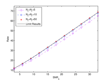
Figure 3: Rate versus $\mbox{SNR}_{a}$ for different numbers of antennas.

IV Multiplexing Gain Analysis and Diversity-Multiplexing Tradeoff

IV-A Multiplexing Gain Analysis

Definition 1

Let $\bar{\gamma}=\frac{1}{L_{s}}\sum_{l=1}^{Ls}\tilde{\gamma}_{l}$. The distributed MIMO system is said to achieve spatial multiplexing gain $G_{m}$ if its ergodic date rate with optimal power allocation satisfies

$$G_{m}(\bar{R}_{o})=\lim_{\bar{\gamma}\to\infty}\frac{\bar{R}_{o}(\bar{\gamma})}{\log_{2}\bar{\gamma}}.$$ (42)

Theorem 2

Assume that both sets $\{\tilde{\mathbf{a}}_{r}(\phi^{rl}_{ij},\theta^{rl}_{ij})\}$ and $\{\tilde{\mathbf{a}}_{t}(\phi^{tl}_{ij},\theta^{tl}_{ij})\}$ are orthogonal vector sets when $N_{r}$ and $N_{t}$ are very large. Assume that $N_{r}$ and $N_{t}$ are always very large but fixed and finite when $\bar{\gamma}\to\infty$. Let $N_{s}\leq L_{s}$. Then the spatial multiplexing gain is given by

$$G_{m}(\bar{R}_{o})=N_{s}.$$ (43)

Proof: We first consider the simple homogeneous case with $\tilde{\gamma}_{1}=\tilde{\gamma}_{2}=\ldots=\tilde{\gamma}_{L_{s}}=\tilde{\gamma}$ and derive the spatial multiplexing gain with respect to $\bar{R}_{eh}$. In this case, $\bar{\gamma}=\tilde{\gamma}$. Obviously,

$$G_{m}(\bar{R}_{eh})=\lim_{\bar{\gamma}\to\infty}\frac{\bar{R}_{eh}(\bar{\gamma})}{\log_{2}\bar{\gamma}}=\sum_{l=1}^{N_{s}}\lim_{\bar{\gamma}\to\infty}\frac{\bar{R}_{eh}^{l}(\bar{\gamma})}{\log_{2}\bar{\gamma}}.$$ (44)

For the $l$th data stream, under the condition of very large $N_{t}$ and $N_{r}$, the individual ergodic rate can be written as

$$R_{eh}^{(l)}(\bar{\gamma})=\mathbb{E}\log_{2}(1+\bar{\gamma}|\tilde{\beta}_{l}|^{2}).$$ (45)

Noting that

$$\mathbb{E}\log_{2}(|\tilde{\beta}_{l}|^{2})\leq\mathbb{E}\log_{2}(1+|\tilde{\beta}_{l}|^{2})=R_{eh}^{(l)}(1)$$ (46)

and $R_{eh}^{(l)}(1)$ is a finite value, we can have that

$$G_{m}^{(l)}(\bar{R}_{eh}) = \lim_{\bar{\gamma}\to\infty}\frac{R_{eh}^{(l)}(\bar{\gamma})}{\log_{2}\bar{\gamma}}$$ (47)

$$= \lim_{\bar{\gamma}\to\infty}\frac{\log_{2}\bar{\gamma}+\mathbb{E}\log_{2}(|\tilde{\beta}_{l}|^{2})}{\log_{2}\bar{\gamma}}$$

$$= 1.$$

Therefore, $G_{m}(\bar{R}_{eh})=\sum_{l=1}^{N_{s}}G_{m}^{(l)}(\bar{R}_{eh})=N_{s}$.

Now we consider the general inhomogeneous case with equal power allocation. Because $c_{min}=\tilde{\gamma}_{min}/\bar{\gamma}$ and $c_{max}=\tilde{\gamma}_{max}/\bar{\gamma}$ be finite when $\bar{\gamma}\to\infty$. Consequently, it readily follows that both of the two systems with the achievable rates $\bar{R}_{eh}(\tilde{\gamma}_{min})$ and $\bar{R}_{eh}(\tilde{\gamma}_{max})$ can achieve a multiplexing gain of $G_{m}(\bar{R}_{eh})=N_{s}$. So we conclude from (41) that the distributed MIMO system with the achievable rate $\bar{R}_{e}(\bar{\gamma})$ can achieve a multiplexing gain of $G_{m}(\bar{R}_{e})=N_{s}$.

Finally, it can be readily shown that the system with the optimal achievable rate $\bar{R}_{o}(\bar{\gamma})$ can only achieve multiplexing gain $G_{m}(\bar{R}_{o})=N_{s}$ since both of the equal power allocation systems with the achievable rates $\bar{R}_{e}(P/N_{s})$ and $\bar{R}_{e}(P)$ have the same spatial multiplexing gain $N_{s}$. $\square$

Corollary 1

Assume that for any $i$ and $j$, the average number of propagation paths $\bar{L}_{ij}=\bar{L}$ . Then the distributed massive MIMO system can obtain an average maximum spatial multiplexing gain of $K_{r}K_{t}\bar{L}$.

Remark 5: Corollary 1 means that compared to the co-located antenna architecture, using the distributed antenna-subarray architecture can statistically scale up the maximum multiplexing gain proportionally to $K_{r}K_{t}$.

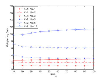
Figure 4: Multiplexing gain versus $\mbox{SNR}_{a}$ for different numbers of data streams.

Now we let $N_{t}^{({\rm rf})}=N_{r}^{({\rm rf})}=2N_{s}$[10] and $K_{r}=K_{t}=K$, and set $L_{ij}=L=3$ and $N_{r}=N_{t}=50$. We consider the homogeneous case and define $\Psi(\bar{\gamma})=\frac{\bar{R}_{eh}(\bar{\gamma})}{\log_{2}\bar{\gamma}}$. In order to verify Theorem 2, Fig.4 plots the curves of $\Psi(\bar{\gamma})$ versus $\mbox{SNR}_{a}=\bar{\gamma}$ for different numbers of data streams, namely, $N_{s}=1,2,3$ when $K=1$ and $N_{s}=3,6,12$ when $K=2$. It can be seen that for any given $N_{s}$, the function $\Psi(\bar{\gamma})$ converges to the limit value $N_{s}$ as $\bar{\gamma}$ grows large. This observation is expected and agrees with Theorem 2.

IV-B Diversity-Multiplexing Tradeoff

The previous subsection shows how much the maximal spatial multiplexing gain we can extract for a distributed mmWave-massive MIMO system while our previous work in [32] indicates how much the maximal spatial diversity gain we can extract. However, maximizing one type of gain will possibly result in minimizing the other. Therefore, we need to bridge between these two extremes in order to simultaneously obtain both types of gains. We firstly give the precise definition of diversity gain before we carry on the analysis.

Definition 2

Let $\bar{\gamma}=\frac{1}{L_{s}}\sum_{l=1}^{Ls}\tilde{\gamma}_{l}$. With an optimal power allocation, the distributed MIMO system is said to achieve spatial diversity gain $G_{d}$ if its average error probability satisfies

$$G_{d}(\bar{P}_{e})=-\lim_{\bar{\gamma}\to\infty}\frac{\log_{2}\bar{P}_{e}(\bar{\gamma})}{\log_{2}\bar{\gamma}}.$$ (48)

or its outage probability satisfies

$$G_{d}(\bar{P}_{out})=-\lim_{\bar{\gamma}\to\infty}\frac{\log_{2}\bar{P}_{out}(\bar{\gamma})}{\log_{2}\bar{\gamma}}.$$ (49)

With the help of a result of diversity analysis in [32], we can derive the following DMT result.

Theorem 3

Assume that both sets $\{\tilde{\mathbf{a}}_{r}(\phi^{rl}_{ij},\theta^{rl}_{ij})\}$ and $\{\tilde{\mathbf{a}}_{t}(\phi^{tl}_{ij},\theta^{tl}_{ij})\}$ are orthogonal vector sets when $N_{r}$ and $N_{t}$ are very large. For a given $d\in[0,L_{s}]$, by using optimal power allocation, the distributed MIMO system can reach the following maximum spatial multiplexing gain at diversity gain $G_{d}=d$

$$G_{m}=\sum_{l=1}^{L_{s}}(1-\frac{d}{L_{s}-l+1})^{+}.$$ (50)

Proof: We first consider the simple case where the distributed system is the one with equal power allocation and the channel is the one with homogeneous large scale fading coefficients. The distributed system has $L_{s}$ available link paths in all. For the $l$th best path, its individual maximum diversity gain is equal to $G_{d}^{(l)}=L_{s}-l+1$ [32]. Due to the fact that each path can not obtain a multiplexing gain of $G_{m}^{(l)}>1$ [31], we therefore design its target data rate $R^{(l)}=r_{l}\log_{2}\bar{\gamma}$ with $0\leq r_{l}\leq 1$. Then the individual outage probability is expressed as

$$P_{out}^{(l)} = \mathbb{P}(\log_{2}(1+\bar{\gamma}|\tilde{\beta}_{l}|^{2})<r_{l}\log_{2}\bar{\gamma})$$ (51)

$$= \mathbb{P}(|\tilde{\beta}_{l}|^{2}<\frac{{\bar{\gamma}}^{r_{l}}-1}{\bar{\gamma}}).$$

From [37], [38], the PDF of the parameter $\mu=|\tilde{\beta}_{l}|^{2}$ can be written as

$$f_{\mu}=a\mu^{L_{s}-l}+o(\mu^{L_{s}-l})$$ (52)

where $a$ is a positive constant. So $P_{out}^{(l)}$ can be rewritten as

$$P_{out}^{(l)}=(c\bar{\gamma})^{-(L_{s}-l+1)(1-r_{l})}+o((\bar{\gamma})^{-(L_{s}-l+1)(1-r_{l})})$$ (53)

where $c$ is a positive constant. This means that this path now can obtain diversity gain

$$G_{d}^{(l)}=(L_{s}-l+1)(1-r_{l}).$$ (54)

Since the distributed system requires its diversity gain $G_{d}\geq d$, this implies that

$$G_{d}^{(l)}=(L_{s}-l+1)(1-r_{l})\geq d$$ (55)

or say

$$r_{l}\leq(1-\frac{d}{L_{s}-l+1})^{+}.$$ (56)

To this end, under the condition that the diversity gain satisfies $G_{d}=d$, the maximum spatial multiplexing gain of the distributed system must be equal to

$$G_{m}(\bar{R}_{eh})=\sum_{l=1}^{L_{s}}r_{l}=\sum_{l=1}^{L_{s}}(1-\frac{d}{L_{s}-l+1})^{+}.$$ (57)

This should be noticed that in order to achieve the maximum spatial multiplexing gain given in (57), the distributed MIMO system must dynamically choose the number of data streams $N_{s}$ by using (56).

This has proved that (50) holds under the special case. Furthermore, we readily show that for a general case, the $l$th best path can also reach a maximum diversity gain of $L_{s}-l+1$. So applying (41) and (29) leads to the desired result. $\square$

Remark 6: When $d$ is an integer, $G_{m}(d)$ can be expressed simply. In particular, $G_{m}(0)=L_{s}$ if $d=0$; $G_{m}(1)=\sum_{l=1}^{L_{s}-1}\frac{L_{s}-l}{L_{s}-l+1}$ if $d=1$; $G_{m}(L_{s}-1)=\frac{1}{L_{s}}$ if $d=L_{s}-1$; $G_{m}(L_{s})=0$ if $d=L_{s}$. In general, if $d=L_{s}-N_{s}+1$ for a given integer $N_{s}\leq L_{s}$, then

$$G_{m}(L_{s}-N_{s}+1)=\sum_{l=1}^{N_{s}-1}\frac{N_{s}-l}{L_{s}-l+1}.$$ (58)

The function $G_{m}(d)$ is plotted in Fig.5. Note that $G_{m}(L_{s}-N_{s})-G_{m}(L_{s}-N_{s}+1)=\sum_{l=1}^{N_{s}}\frac{1}{L_{s}-l+1}.$ Generally, when $d\in[L_{s}-N_{s},L_{s}-N_{s}+1)$ , the multiplexing gain is given by

$$G_{m}(d)=N_{s}-\sum_{l=1}^{N_{s}}\frac{d}{L_{s}-l+1}.$$ (59)

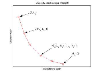
Figure 5: Diversity-multiplexing tradeoff $G_{m}(d)$ for a general integer $d$.

Example 1: We set that $K_{t}=K_{r}=2$ and $L_{ij}=L=3$ . So $L_{s}=12$. The DMT curve with fractional multiplexing gains is shown in Fig.6. If the multiplexing gains be limited to integers, the corresponding DMT curve is also plotted in Fig.6 for comparison.

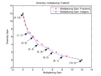
Figure 6: Diversity-multiplexing tradeoff when $L=3$ and $K_{t}=K_{r}=2$.

V DMT Analysis with the Conventional Partially-Connected Structure

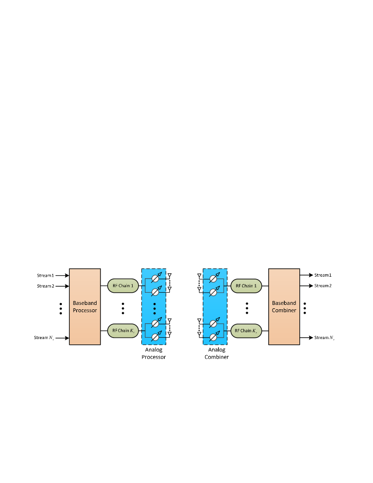
Figure 7: Block diagram of a mmWave massive MIMO system with the conventional partially-connected RF architecture.

The previous section has analyzed the multiplexing gain for the massive MIMO system with the general fully-connected RF architecture and given a DMT characterization. This section focuses on a massive MIMO system employing the conventional partially-connected RF architecture as illustrated in Fig. 7. Here the transmitter equipped with $K_{t}$ RF chains sends $N_{s}$ data streams to the receiver equipped with $K_{r}$ RF chains. Each RF chain at the transmitter or receiver is connected to only one RAU. It is assumed that $N_{s}\leq\min\{K_{t},K_{r}\}$. The numbers of antennas per each RAU at the transmitter and receiver are fixed as $N_{t}$ and $N_{r}$, respectively. Note that $N_{t}\gg N_{s}$ and $N_{r}\gg N_{s}$. Both the transmitter and receiver employ very small digital processors and very large analog processors, represented respectively by $\mathbf{W}_{t}$ and $\mathbf{F}_{t}$ for the transmitter, and $\mathbf{W}_{r}$ and $\mathbf{F}_{r}$ for the receiver.

As before, denote by $\mathbf{s}$ the transmitted symbol vector, by $\mathbf{H}$ the fading channel matrix, and by $\mathbf{n}$ the noise vector. Then at the receiver the processed signal vector $\mathbf{z}$ is given by (3), whereas $\mathbf{H}$ is described as in (5). Due to the partially-connected RF architecture, the analog processors $\mathbf{F}_{t}$ and $\mathbf{F}_{r}$ are block diagonal matrices, expressed as

$$\mathbf{F}_{t}=\mathrm{diag}\{\mathbf{f}_{t1},\mathbf{f}_{t2},\ldots,\mathbf{f}_{tK_{t}}\}$$ (60)

and

$$\mathbf{F}_{r}=\mathrm{diag}\{\mathbf{f}_{r1},\mathbf{f}_{r2},\ldots,\mathbf{f}_{rK_{r}}\}$$ (61)

where $\mathbf{f}_{ti}$ denotes the $N_{t}\times 1$ steering vector of phases for the $i$th RAU at the transmitter, and $\mathbf{f}_{rj}$ the $N_{r}\times 1$ steering vector of phases for the $j$th RAU at the transmitter.

Now let $K_{m}=\min\{K_{r},K_{t}\}$ . Obviously, the distributed system at most has $K_{m}$ available link paths. For the $l$th best path, its individual maximum diversity gain is denoted as $G_{d}^{(l)}$. In general, we can compute $G_{d}^{(l)}$ by an algorithm. If $L_{ij}=L$ for any $i$ and $j$, it follows from [32] that

$$G_{d}^{(l)}=(K_{t}-l+1)(K_{r}-l+1)L,\;\;l=1,2,\ldots,K_{m}.$$ (62)

Theorem 4

Consider the case that the antenna array configuration at each RAU is ULA. For a given $d\in[0,L_{s}]$, by using optimal power allocation, the distributed MIMO system with the partially-connected RF architecture can reach the following maximum spatial multiplexing gain at diversity gain $G_{d}=d$

$$G_{m}=\sum_{l=1}^{K_{m}}(1-\frac{d}{G_{d}^{(l)}})^{+}.$$ (63)

Proof: Following the same steps in the derivation of $G_{m}$ in Theorem 3, we can readily obtain (63). $\square$

Remark 7: Furthermore, we suppose that $L_{ij}=L$ for any $i$ and $j$. Then the distributed system in the limit of large $N_{t}$ and $N_{r}$ can reach the following maximum spatial multiplexing gain at diversity gain $G_{d}=d$

$$G_{m}=\sum_{l=1}^{K_{m}}(1-\frac{d}{(K_{t}-l+1)(K_{r}-l+1)L})^{+}.$$ (64)

VI DMT Analysis for the Multiuser Scenario

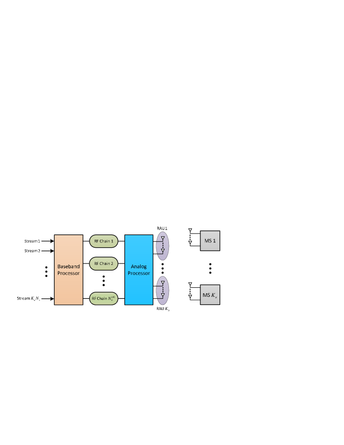
Figure 8: Block diagram of a multiuser mmWave system with distributed antenna arrays.

This section considers the downlink communication in a multiuser massive MIMO system as illustrated in Fig. 8. Here the base station (BS) employs $K_{b}$ RAUs with each having $N_{b}$ antennas and $N_{b}^{({\rm rf})}$ RF chains to transmit data streams to $K_{u}$ mobile stations. Each mobile station (MS) is equipped with $N_{u}$ antennas and $N_{u}^{({\rm rf})}$ RF chains to support the reception of its own $N_{s}$ data streams. This means that there is a total of $K_{u}N_{s}$ data streams transmitted by the BS. The numbers of data streams are constrained as $K_{u}N_{s}\leq N_{b}^{({\rm rf})}\leq K_{b}N_{b}$ for the BS, and $N_{s}\leq N_{u}^{({\rm rf})}\leq N_{u}$ for each MS.

At the BS, denote by $\mathbf{F}_{b}$ the $K_{b}N_{b}\times N_{b}^{({\rm rf})}$ RF precoder and by $\mathbf{W}_{b}$ the $N_{b}^{({\rm rf})}\times N_{s}K_{u}$ baseband precoder. Then under the narrowband flat fading channel model, the received signal vector at the $i$th MS is given by

$$\mathbf{y}_{i}=\mathbf{H}_{i}\mathbf{F}_{b}\mathbf{W}_{b}\mathbf{s}+\mathbf{n}_{i},\;i=1,2,\ldots,K_{u}$$ (65)

where $\mathbf{s}$ is the signal vector for all $K_{u}$ mobile stations, which satisfies $\mathbb{E}[\mathbf{s}\mathbf{s}^{H}]=\frac{P}{K_{u}N_{s}}\mathbf{I}_{K_{u}N_{s}}$ and $P$ is the average total transmit power. The $N_{u}\times 1$ vector $\mathbf{n}_{i}$ represents additive white Gaussian noise, whereas the $N_{u}\times K_{b}N_{b}$ matrix $\mathbf{H}_{i}$ is the channel matrix corresponding to the $i$th MS, whose entries $\mathbf{H}_{ij}$ are described as in Section II. Furthermore, the signal vector after combining can be expressed as

$$\mathbf{z}_{i}=\mathbf{W}_{ui}^{H}\mathbf{F}_{ui}^{H}\mathbf{H}_{i}\mathbf{F}_{b}\mathbf{W}_{b}\mathbf{s}+\mathbf{W}_{ui}^{H}\mathbf{F}_{ui}^{H}\mathbf{n}_{i},\;i=1,2,\ldots,K_{u}$$ (66)

where $F_{ui}$ is the $N_{u}\times N_{u}^{({\rm rf})}$ RF combining matrix and $\mathbf{W}_{ui}$ is the $N_{u}^{({\rm rf})}\times N_{s}$ baseband combining matrix for the $i$th MS.

Theorem 5

Assume that all antenna array configurations for the downlink transmission are ULA. For the $i$th user, let $L_{s}^{(i)}=\sum_{j=1}^{K_{b}}L_{ij}$ and $0\leq d^{(i)}\leq L_{s}^{(i)}$. In the limit of large $N_{b}$ and $N_{u}$, the $i$th user can achieve the following maximum spatial multiplexing gain when its individual diversity gain satisfies $G_{d}^{(i)}=d^{(i)}$

$$G_{m}^{(i)}=\sum_{l=1}^{L_{s}^{i}}(1-\frac{d^{(i)}}{L_{s}^{(i)}-l+1})^{+}.$$ (67)

Proof: For the downlink transmission in a massive MIMO multiuser system, the overall equivalent multiuser basedband channel can be written as

$$\mathbf{H}_{\rm eq}=\left[\begin{array}[]{llll}\mathbf{F}_{u1}^{H}&\mathbf{0}&\cdots&\;\;\mathbf{0}\\ \mathbf{0}&\mathbf{F}_{u2}^{H}&\cdots&\;\;\mathbf{0}\\ \vdots&\vdots&\ddots&\;\;\vdots\\ \mathbf{0}&\mathbf{0}&\cdots&\mathbf{F}_{uK_{u}}^{H}\end{array}\right]\left[\begin{array}[]{l}\mathbf{H}_{1}\\ \mathbf{H}_{2}\\ \vdots\\ \mathbf{H}_{K_{u}}\end{array}\right]\mathbf{F}_{b}.$$ (68)

On the other hand, when both $N_{b}$ and $N_{u}$ are very large, it follows easily that both BS and MS array response vector sets are orthogonal sets. Therefore the multiplexing gain for the $i$th user can depend only on the subchannel matrix $\mathbf{H}_{i}$ and the choices of $\mathbf{F}_{ui}$ and $\mathbf{F}_{b}$. The subchannel matrix $\mathbf{H}_{i}$ has a total of $L_{s}^{(i)}$ propagation paths. Similar to the proof of Theorem 2, by employing the optimal RF precoder and combiner for the $i$th user, when its diversity gain satisfies $G_{d}^{i}=d^{(i)}$, the user can achieve a maximum multiplexing gain of

$$G_{m}^{(i)}=\sum_{l=1}^{L_{s}^{(i)}}(1-\frac{d^{(i)}}{L_{s}^{(i)}-l+1})^{+}.$$ (69)

So we obtain the desired result. $\square$

Remark 8: Furthermore, we suppose that $L_{ij}=L$ for any $i$ and $j$ . Let $0\leq d\leq K_{b}L$. Then in the limit of large $N_{b}$ and $N_{u}$, the downlink transmission in the massive MIMO multiuser system can achieve the following maximum spatial multiplexing gain at diversity gain $G_{d}=d$

$$G_{m}=\sum_{i=1}^{K_{u}}G_{m}^{(i)}=K_{u}\sum_{l=1}^{K_{b}L}(1-\frac{d}{K_{b}L-l+1})^{+}.$$ (70)

Remark 9: In a similar fashion, it is easy to prove that the uplink transmission in the massive MIMO multiuser system can also achieve simultaneously a diversity gain of $G_{d}=d$ ($0\leq d\leq K_{b}L$) and a spatial multiplexing gain of

$$G_{m}=K_{u}\sum_{l=1}^{L_{s}}(1-\frac{d}{K_{b}L-l+1})^{+}.$$ (71)

VII Conclusion

This paper has investigated the distributed antenna subarray architecture for mmWave massive MIMO systems and provided the asymptotical multiplexing analysis when the number of antennas at each subarray goes to infinity. In particular, this paper has derived the closed-form formulas of the asymptotical available rate and spatial maximum multiplexing gain under the assumption which the subchannel matrices between transmit and receive antenna subarrays behave independently. The spatial multiplexing gain formula shows that mmWave systems with the distributed antenna architecture can achieve potentially rather larger multiplexing gain than the ones with the conventional co-located antenna architecture. On the other hand, using the distributed antenna architecture can also achieve potentially rather higher diversity gain. For a given mmWave massive MIMO channel, both types of gains can be simultaneously obtained. This paper has finally given a simple DMT tradeoff solution, which provides insights for designing a mmWave massive MIMO system.

References

- [1] T. S. Rappaport et al., “Millimeter wave mobile communications for 5G cellular: It will work!” IEEE Access, vol. 1, pp. 335-349, May 2013.
- [2] A. L. Swindlehurst, E. Ayanoglu, P. Heydari, and F. Capolino, “Millimeter-wave massive MIMO: the next wireless revolution?” IEEE Commun. Mag., vol. 52, no. 9, pp. 56-62, Sep. 2014.
- [3] W. Roh et al., “Millimeter-wave beamforming as an enabling technology for 5G cellular communications: theoretical feasibility and prototype results,” IEEE Commun. Mag., vol. 52, no. 2, pp. 106-113, Feb. 2014.
- [4] O. E. Ayach, R. W. Heath, S. Abu-Surra, S. Rajagopal and Z. Pi, “The capacity optimality of beam steering in large millimeter wave MIMO systems,” in Proc. IEEE 13th Intl. Workshop on Sig. Process. Advances in Wireless Commun. (SPAWC), pp. 100-104, June 2012.
- [5] O. E. Ayach, R. W. Heath, S. Rajagopal, and Z. Pi, “Multimode precoding in millimeter wave MIMO transmitters with multiple antenna sub-arrays,” in Proc. IEEE Glob. Commun. Conf., 2013, pp. 3476-3480.
- [6] J. Singh and S. Ramakrishna, “On the feasibility of beamforming in millimeter wave communication systems with multiple antenna arrays,“ in Proc. IEEE GLOBECOM, 2014, pp. 3802-3808.
- [7] L. Liang, W. Xu and X. Dong, “Low-complexity hybrid precoding in massive multiuser MIMO systems,” IEEE Wireless Commun. Letters, vol.3, no.6, pp. 653-656, Dec. 2014.
- [8] J. A. Zhang, X. Huang, V. Dyadyuk, and Y. J. Guo, “Massive hybrid antenna array for millimeter-wave cellular communications,” IEEE Wire- less Commun., vol. 22, no. 1, pp. 79-87, Feb. 2015.
- [9] W. Ni and X. Dong, “Hybrid Block Diagonalization for Massive Multiuser MIMO Systems,” IEEE Transactions on Communications, vol.64, no.1, pp.201-211, Jan. 2016.
- [10] F. Sohrabi and W. Yu, “Hybrid digital and analog beamforming design for large-scale antenna arrays,” IEEE Journal of Selected Topics in Signal Processing, vol. 10, no. 3, pp. 501-513, Apr. 2016.
- [11] S. He, C. Qi, Y. Wu, and Y. Huang, “Energy-efficient transceiver design for hybrid sub-array architecture MIMO systems,” IEEE Access, vol. 4, pp. 9895-9905, 2016.
- [12] N. Li, Z. Wei, H. Yang, X. Zhang, D. Yang, “Hybrid Precoding for mmWave Massive MIMO Systems With Partially Connected Structure,” IEEE Access, vol. 5, pp. 15142-15151, 2017.
- [13] D. Zhang, Y. Wang, X. Li, W. Xiang, “Hybridly-Connected Structure for Hybrid Beamforming in mmWave Massive MIMO Systems,” IEEE Transactions on Communication, DOI 10.1109/TCOMM.2017.2756882, Sep. 2017.
- [14] N. Song, T. Yang, and H. Sun, “Overlapped subarray based hybrid beamforming for millimeter wave multiuser massive MIMO,” IEEE Signal Processing Letters, vol. 24, no. 5, pp. 550-554, May 2017.
- [15] S. Kutty and D. Sen, “Beamforming for millimeter wave communications: an inclusive surey,” IEEE Communications Surveys & Tutorials, vol. 18, no.2, pp. 949-973, Second Quarter 2016.
- [16] A. F. Molisch, V. V. Ratnam, S. Han, Z. Li, S. L. H. Nguyen, L. Li, and K. Haneda, “Hybrid beamforming for massive MIMO-a survey,” arXiv preprint arXiv: 1609.05078, 2016.
- [17] Z. Pi and F. Khan, “An introduction to millimeter-wave mobile broadband systems,” IEEE Comm. Mag., vol. 49, no. 6, pp.101-107, 2011.
- [18] T. S. Rappaport, F. Gutierrez, E. Ben-Dor, J. N. Murdock, Y. Qiao, and J. I. Tamir, “Broadband millimeter-wave propagation measurements and models using adaptive-beam antennas for outdoor urban cellular communications,” IEEE Trans. Antennas Propag., vol. 61, no. 4, pp. 1850-1859, Apr. 2013.
- [19] V. Raghavan and A. M. Sayeed, “Multi-antenna capacity of sparse multipath channels,” IEEE Trans. Inf. Theory., 2008. [Online]. Available: dune.ece.wisc.edu/pdfs/sp mimo cap.pdf
- [20] V. Raghavan and A. M. Sayeed, “Sublinear capacity scaling laws for sparse MIMO channels,” IEEE Trans. Inf. Theory., vol. 57, no. 1, pp. 345-364, Jan. 2011.
- [21] M. V. Clark, T. M. W. III, L. J. Greenstein, A. J. Rustako, V. Erceg, and R. S. Roman, “Distributed versus centralized antenna arrays in broadband wireless networks,” in Proc. IEEE Veh. Technology Conf. (VTC’01), May 2001, pp. 33-37.
- [22] W. Roh and A. Paulraj, “MIMO channel capacity for the distributed antenna systems,” in IEEE Veh. Technology Conf. (VTC’02), vol. 3, Sept. 2002, pp. 1520-1524.
- [23] L. Dai, “A comparative study on uplink sum capacity with co-located and distributed antennas,” IEEE J. Sel. Areas Commun., vol. 29, no. 6, pp. 1200-1213, June 2011.
- [24] Q.Wang,D. Debbarma, A. Lo, Z. Cao, I. Niemegeers, S. H. de Groot, “Distributed antenna system for mitigating shadowing effect in 60 GHz WLAN,”, wireless Personal Communications, vol. 82, no. 2, pp. 811-832, May 2015.
- [25] S. Gimenez, D. Calabuig, S. Roger, J. F. Monserrat, and N. Cardona, “Distributed hybrid precoding for indoor deployments using millimeter wave band,” Mobile Information Systems, vol. 2017, Article ID 5751809, 12 pages, Oct. 2017.
- [26] L. Zheng and D. N. C. Tse, “Diversity and multiplexing: A fundamental tradeoff in multiple antenna channels,” IEEE Trans. Inform. Theory, vol. 49, pp. 1073-1096, May 2003.
- [27] D. Tse, P. Viswanath, and L. Zheng, “Diversity-multiplexing tradeoff in multiple access channels,” IEEE Trans. Inform. Theory, vol. 50, pp. 1859-1874, Sep. 2004.
- [28] L. Zhao, W. Mo, Y. Ma, and Z. Wang, “Diversity and multiplexing tradeoff in general fading channels,” Electrical and Computer Engineering Department, Iowa State University, Tech. Rep., 2005.
- [29] R. Narasimhan, “Finite-SNR diversity-multiplexing tradeoff for correlated Rayleigh and Rician MIMO channels,” IEEE Transactions on Information Theory, vol.52, no. 9, pp. 3965- 3979, 2006.
- [30] M. Yuksel and E. Erkip, “Multiple-antenna cooperative wireless systems: A diversity-multiplexing tradeoff perspective,” IEEE Trans. Inform. Theory, vol. 53, pp 3371-3393, Oct. 2007.
- [31] D. Tse and P. Viswanath, Fundamentals of Wireless Communication. Cambridge, U.K.: Cambridge Univ. Press, 2007.
- [32] D.-W. Yue, S. Xu, and H.H. Nguyen “Diversity analysis of millimeter-wave massive MIMO systems,” [Online]. Available: http://arxiv.org/abs/1801.00387.
- [33] I. E. Telatar, ”Capacity of multi-antenna Gaussian channels,” European Trans. on Telecomm., vol. 10, pp. 585-596, Nov.-Dec. 1999.
- [34] M. K. Simon and M. -S. Alouini, Digital Communication over Fading Channels, Second Edition New York: John Wiley & Sons, Inc., 2005.
- [35] I. S. Gradshteyn and I. M. Ryzhik, Table of Integrals, Series, and Products, 5th ed. San Diego, CA: Academic Press, 1994.
- [36] H. A. David, Order Statistics, New York, NY: John Wiley & Sons, Inc., 1981.
- [37] Z. Wang and G. B. Giannakis, “A simple and general parameterization quantifying performance in fading channels,” IEEE Trans. Signal Process., vol. 51, no. 8, pp. 1389-1398, Aug. 2003.
- [38] L. G. Ordóñz, , D. P. Palomar, A. Pagès-Zamora, and J. R. Fonollosa, “High-SNR Analytical Performance of Spatial Multiplexing MIMO Systems With CSI,” IEEE Transactions on Signal Processing, Vol.55, no. 11, pp. 5447-5463, Nov. 2007