Study of the process $e^{+}e^{-}\rightarrow\pi^{+}\pi^{-}\eta$ using initial state radiation

Abstract

We study the process $e^{+}e^{-}\rightarrow\pi^{+}\pi^{-}\eta\gamma$, where the photon is radiated from the initial state. About 8000 fully reconstructed events of this process are selected from the BABAR data sample with an integrated luminosity of 469 $\mbox{\,fb}^{-1}$. Using the $\pi^{+}\pi^{-}\eta$ invariant mass spectrum we measure the $e^{+}e^{-}\rightarrow\pi^{+}\pi^{-}\eta$ cross section in the $e^{+}e^{-}$ center-of-mass energy range from 1.15 to 3.5 $\mathrm{\,Ge\kern-1.00006ptV}$. The cross section is well described by the Vector-Meson Dominance model with four $\rho$-like states. We observe $49\pm 9$ events of the $J/\psi$ decay to $\pi^{+}\pi^{-}\eta$, and measure the product $\Gamma_{J/\Psi\rightarrow e^{+}e^{-}}{\cal B}_{J/\Psi\rightarrow\pi^{+}\pi^{-}\eta}=2.34\pm 0.43_{\text{stat}}\pm 0.16_{\text{syst}}$ $\mathrm{\,e\kern-1.00006ptV}$.

I Introduction

A photon radiated from the initial state in the reaction $e^{+}e^{-}\rightarrow\gamma+\text{hadrons}$ effectively reduces the electron-positron collision energy. This allows the study of hadron production over a wide range of $e^{+}e^{-}$ center-of-mass energies in a single experiment. The possibility of exploiting initial-state-radiation (ISR) events to measure low-energy cross sections at high-luminosity $B$ factories is discussed in Refs. NLO_ISR ; ISRprinciple ; ISRprinciple1 and motivates the study described in this paper. The study of ISR events at the $B$ factories provides independent cross section measurements and contributes to understanding low-mass hadron spectroscopy.

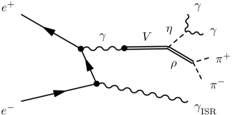
Figure 1: The Feynman diagram for the process $e^{+}e^{-}\rightarrow\gamma_{\rm ISR}\pi^{+}\pi^{-}\gamma\gamma$ via the $\rho\eta$ intermediate state in the Vector-Meson Dominance model.

In $e^{+}e^{-}$ annihilations, final states like $\pi^{+}\pi^{-}\eta$ with positive G-parity must result from the isovector part of the hadronic current. Within the context of the Vector-Meson Dominance (VMD) model NNAChasov , the $e^{+}e^{-}\rightarrow\pi^{+}\pi^{-}\eta$ process can be described by the Feynman diagram in Fig. 1, where V represents any $\rho$ resonance, and $\rho$ is any accessible $\rho$ resonance. The process is important for the determination of the parameters of $\rho$ resonances, gives a sizable contribution to the total hadronic cross section in the energy range 1.35–1.85 GeV. Additionally, results of the research can be used to test the relation between the $e^{+}e^{-}\rightarrow\pi^{+}\pi^{-}\eta$ cross section and the spectral function for the decay $\tau^{-}\rightarrow\pi^{-}\pi^{0}\eta\nu_{\tau}$ predicted under the conserved vector current (CVC) hypothesis CVCEidelman .

The process $e^{+}e^{-}\rightarrow\pi^{+}\pi^{-}\eta$ was studied in several direct $e^{+}e^{-}$ experiments at energies from threshold to 2.4 GeV: DM1 DM1 , ND ND , DM2 DM2 , CMD-2 CMD-2 , and SND 2pieta_SND ; 2pieta_SND2014 . This process was also studied by BABAR using the decay mode $\eta\rightarrow\pi^{-}\pi^{+}\pi^{0}$ with the ISR technique. The BABAR study was based on a 239 $\mbox{\,fb}^{-1}$ data sample BaBar2007 and reached 3 GeV. The cross section and $\pi^{+}$ $\pi^{-}$ mass distributions were consistent with VMD. A theoretical study of the process $e^{+}e^{-}\rightarrow\pi^{+}\pi^{-}\eta$ within VMD and Nambu-Jona-Lasinio chiral approaches was performed in Ref. NNAChasov and Refs. NJL ; ResonChirTh , respectively.

This paper reports a study of the $\pi^{+}\pi^{-}\eta$ hadronic final state with $\eta\rightarrow 2\gamma$ produced together with a energetic photon that is assumed to result from ISR. The invariant mass of the hadronic system determines the reduced effective $e^{+}e^{-}$ center-of-mass (c.m.) energy ($E_{\rm c.m.}$ $\equiv m_{\pi^{+}\pi^{-}\eta}c^{2}$), and we measure the $e^{+}e^{-}\rightarrow\pi^{+}\pi^{-}\eta$ cross section in the range $1.15<E_{\rm c.m.}<3.5$ $\mathrm{\,Ge\kern-1.00006ptV}$. The different $\eta$ decay mode makes this independent of our previous work. We fit the results using the VMD model and extract $\rho$ resonances parameters, and we calculate a $\tau\rightarrow\pi^{+}\pi^{0}\eta\nu_{\tau}$ branching fraction under the CVC hypothesis.

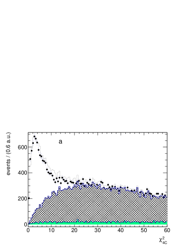
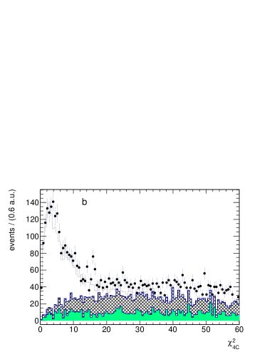
Figure 2: (color online) The distributions of $\chi^{2}_{\rm 4C}$ for events from the invariant mass ranges $1.15<m_{\pi^{+}\pi^{-}\eta}<2.00$ ${\mathrm{\,Ge\kern-1.00006ptV\!/}c^{2}}$ (a) and $2.0<m_{\pi^{+}\pi^{-}\eta}<3.5$ ${\mathrm{\,Ge\kern-1.00006ptV\!/}c^{2}}$ (b). The points with error bars are data. The open histogram represents the sum of the simulated distributions for signal and backgrounds events. The shaded histogram represents non-ISR background, while the hatched area shows ISR background.

II The BABAR detector and data set

The data used in this analysis were collected with the BABAR detector at the PEP-II asymmetric-energy $e^{+}e^{-}$ collider at the SLAC National Accelerator Laboratory. The integrated luminosity of 468.6 $\mbox{\,fb}^{-1}$ lumi used in this analysis comprises 424.7 $\mbox{\,fb}^{-1}$ collected at the $\mathchar 28935\relax(4S)$ resonance, and 43.9 $\mbox{\,fb}^{-1}$ collected 40 MeV below the peak.

The BABAR detector is described in detail elsewhere Detector ; Detector1 . Charged particles are reconstructed using a tracking system, which comprises a silicon vertex tracker (SVT) and a drift chamber (DCH) inside a 1.5 T solenoid magnet. Separation of pions and kaons is accomplished by means of the detector of internally reflected Cherenkov light (DIRC) and energy-loss measurements in the SVT and DCH. The energetic ISR photon and photons from $\pi^{0}$ and $\eta$ decays are detected in the electromagnetic calorimeter (EMC). Muon identification is provided by the instrumented flux return of the magnetic field.

To study the detector acceptance and efficiency, a special package of programs for simulation of ISR processes was developed based on the approach suggested in Ref. EVA . Multiple collinear soft-photon emission from the initial $e^{+}e^{-}$ state is implemented with the structure-function technique structuremethod , while additional photon radiation from the final-state particles (FSR) is simulated using the PHOTOS package photos . The precision of the radiative-correction simulation does not contribute more than 1% uncertainty to the efficiency calculation.

The process $e^{+}e^{-}\rightarrow\pi^{+}\pi^{-}\eta\gamma$ is simulated assuming the intermediate $\rho(770)\eta$ hadronic state. Generated events are processed through the detector response simulation GEANT4 and then reconstructed using the same procedure as the real data. Variations in the detector and background conditions are taken into account in the simulation.

We simulate the background ISR processes $e^{+}e^{-}\rightarrow K^{+}K^{-}\eta\gamma$, $\pi^{+}\pi^{-}\pi^{0}\pi^{0}\gamma$, $\pi^{+}\pi^{-}3\pi^{0}\gamma$, $\pi^{+}\pi^{-}\pi^{0}\eta\gamma$, and $\pi^{+}\pi^{-}\pi^{0}\gamma$, and non-ISR processes $e^{+}e^{-}\rightarrow\tau^{+}\tau^{-}$ and $e^{+}e^{-}\rightarrow q\overline{q}$ $(q=u,d,s)$. The latter process is generated using the Jetset 7.4 udssim event generator.

III Event selection and kinematic fit

Preliminary selection criteria require detection of a high-energy photon with a c.m. energy greater than 3 $\mathrm{\,Ge\kern-1.00006ptV}$, at least two charged-particle tracks, and at least two additional photons with invariant mass near the $\eta$ mass, in the range 0.44–0.64 ${\mathrm{\,Ge\kern-1.00006ptV\!/}c^{2}}$. Each of the photons is required to have an energy greater than 100 $\mathrm{\,Me\kern-1.00006ptV}$ and a polar angle in the range 0.3–2.1 radians. The photon with the highest c.m. energy is assumed to be from ISR. Charged-particle tracks are required to originate within 0.25 cm of the beam axis and within 3 cm of the nominal collision point along the axis. Each of the tracks is required to have momentum higher than 100 ${\mathrm{\,Me\kern-1.00006ptV\!/}c}$, and be in the polar angle range 0.4–2.4 radians. Additionally, the tracks are required to be not identified as kaons or muons. If there are three or more tracks, the oppositely charged pair with closest distance to the interaction region is used for the further analysis. The selected candidate events are subjected to a 4C kinematic fit under the $e^{+}e^{-}\rightarrow\pi^{+}\pi^{-}3\gamma$ hypothesis, which includes four constraints of energy-momentum balance. The common vertex of the charged-particle tracks is used as the point of origin for the detected photons. There is no constraint on the $\eta$ candidate mass, since this will be used below to extract the number of signal events. Monte-Carlo (MC) simulation and data samples contain a significant number of false photons arising from split-off charged-pion EMC clusters and beam-generated background, as well as additional ISR or FSR photons. For events with more than three photons we perform a kinematic fit for all photon-pair combinations not including the ISR photon, and choose the combination with the lowest value of $\chi^{2}_{\rm 4C}$. The parameter $\chi^{2}_{\rm 4C}$ is used to discriminate between signal and background events.

Since the production of the two-pion system is predominantly via $\rho$-meson intermediate states we require that the invariant mass of the two pions, $m_{2\pi}$, is greater than 0.4 GeV/c². Because of very different background conditions, the $\pi^{+}\pi^{-}\eta$ invariant mass interval under study is divided into two regions: $1.15<m_{\pi^{+}\pi^{-}\eta}<2.00$ ${\mathrm{\,Ge\kern-1.00006ptV\!/}c^{2}}$ (I) and $2.0<m_{\pi^{+}\pi^{-}\eta}<3.5$ ${\mathrm{\,Ge\kern-1.00006ptV\!/}c^{2}}$ (II). Two additional selection conditions are used for Region II: the energies of photons from the $\eta$ decay are required to be greater than 200 MeV and $m_{\pi^{\pm}\gamma_{\text{ISR}}}>1$ GeV/c², where $m_{\pi^{\pm}\gamma_{\text{ISR}}}$ is the invariant mass of the charged pion and the ISR photon. The latter condition rejects $e^{+}e^{-}\rightarrow\tau^{+}\tau^{-}$ background events with one of the $\tau$ decaying into $\rho^{\pm}\nu\rightarrow\pi^{\pm}\pi^{0}\nu$, where an energetic photon, considered as $\gamma_{\rm ISR}$, arises from $\pi^{0}$ decay. In this case the spectrum of invariant mass of the most energetic photon and one of the selected charged pions is peaked near the $\rho$ mass.

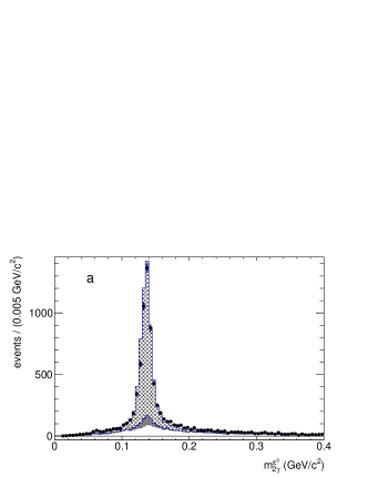
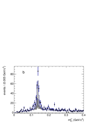
Figure 3: The distribution of $m^{\pi^{0}}_{2\gamma}$ for Region I (a) and for Region II (b). The points with error bars are data. The open histogram represents signal simulation, the shaded and hatched areas shows simulated non-ISR and ISR background contributions, respectively.

The $\chi^{2}_{\rm 4C}$ distributions for events from Region I and Region II are shown in Fig. 2. The points with error bars represent data, while the histograms show, cumulatively, the contributions of simulated non-ISR background (shaded), ISR background (hatched), and signal $e^{+}e^{-}\rightarrow\pi^{+}\pi^{-}\eta\gamma$ events (open histogram). For background, the distributions are normalized to the expected numbers of events calculated using known experimental cross sections, in particular, 2pi2pi0datababar for $e^{+}e^{-}\rightarrow\pi^{+}\pi^{-}\pi^{0}\pi^{0}\gamma$, babar2keta for $e^{+}e^{-}\rightarrow K^{+}K^{-}\eta\gamma$, snd3pieta for $e^{+}e^{-}\rightarrow\pi^{+}\pi^{-}\pi^{0}\eta\gamma$ and tautausim for $e^{+}e^{-}\rightarrow\tau^{+}\tau^{-}$. For the non-ISR $e^{+}e^{-}\rightarrow q\overline{q}$ background, the expected number is corrected to take into account the observed data-MC simulation difference (see below). The signal distribution is normalized in such a way that the total simulated distribution matches the first seven bins of the data distribution. It is seen that the simulated backgrounds at $\chi^{2}_{\rm 4C}>20$ are adequate in the lower-mass $m_{\pi^{+}\pi^{-}\eta}$ region, but not in the higher. The conditions $\chi^{2}_{\rm 4C}<25$ and $\chi^{2}_{\rm 4C}<15$ are used for Region I and II, respectively.

Most background processes contain neutral pions in the final state. To suppress this background, we check all possible combinations of pairs of photons with energy higher than 100 MeV and choose the one with invariant mass ($m^{\pi^{0}}_{2\gamma}$) closest to the $\pi^{0}$ mass. The obtained $m^{\pi^{0}}_{2\gamma}$ distribution is shown in Fig. 3. We apply the requirement $m^{\pi^{0}}_{2\gamma}>0.16$ GeV/c². With these conditions, 11469 data events are selected.

The remaining simulated ISR background is still dominated by the $e^{+}e^{-}\rightarrow\pi^{+}\pi^{-}\pi^{0}\pi^{0}\gamma$ process. In the non-ISR background, about 50% of events come from the process $e^{+}e^{-}\rightarrow q\overline{q}\rightarrow\pi^{+}\pi^{-}\pi^{0}\eta$, which imitates the process under study when one of photons from the $\pi^{0}$ decay is soft and the other is identified as the ISR photon. Such events preferentially have a small $\chi^{2}_{\rm 4C}$ like signal events. Remaining non-ISR events come from the process $e^{+}e^{-}\rightarrow q\overline{q}\rightarrow\pi^{-}\pi^{+}\pi^{0}\pi^{0}$ or from processes with higher neutral particle multiplicity ($e^{+}e^{-}\rightarrow q\overline{q}\rightarrow\pi^{+}\pi^{-}\pi^{0}\pi^{0}\pi^{0}$, $e^{+}e^{-}\rightarrow q\overline{q}\rightarrow\pi^{-}\pi^{+}\eta\pi^{0}\pi^{0}$, etc.), and have a uniform $\chi^{2}_{\rm 4C}$ distribution. To check the quality of the Jetset simulation, we select non-ISR events in data and simulation using the following procedure.

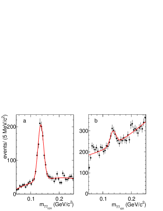
Figure 4: The distributions of the invariant mass for all combinations of the ISR-photon candidate with any other photon in an event in $e^{+}e^{-}\rightarrow q\bar{q}$ simulation (a) and data (b). The curves are the results of the fits described in the text.

We remove the condition $m^{\pi^{0}}_{2\gamma}>0.16$ GeV/c² and modify the $\chi^{2}_{\rm 4C}$ condition to $\chi^{2}_{\rm 4C}<100$. The invariant masses for all combinations of the ISR-photon candidate with any other photon in an event are calculated. The mass distributions are shown in Fig. 4 for simulated $q\bar{q}$ and data events. The $\pi^{0}$ peak is clearly seen both in data and in simulation, indicating the presence of non-ISR processes. The distributions are fitted with a sum of a Gaussian function describing the $\pi^{0}$ resolution function and a second-order polynomial. In the fit to the data distribution, the parameters of the Gaussian function are fixed to the values obtained in the fit to the simulated distribution. The ratio of the number of data events in the $\pi^{0}$ peak to that expected from the Jetset simulation is found to be $0.70\pm 0.05$. This data-MC simulation scale factor is an average over the mass range $1.15<m_{\pi^{+}\pi^{-}\eta}<3.5$ ${\mathrm{\,Ge\kern-1.00006ptV\!/}c^{2}}$. We do not observe a $m_{\pi^{+}\pi^{-}\eta}$ dependence of the scale factor at the level of the available statistics. After the simulation normalization the number of $e^{+}e^{-}\rightarrow q\overline{q}\rightarrow\pi^{+}\pi^{-}\pi^{0}\eta$ events satisfying our standard selection criteria is estimated to be 171$\pm$12.

\begin{overpic}[scale={0.4}]{m2g_1.1_2.3.eps} \end{overpic}

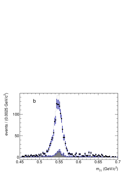
Figure 5: The two-photon invariant mass distribution for events from Region I (a), and Region II (b) after all selections. The points with error bars represent data. The histograms cumulatively show simulated contributions for peaking background (shaded), nonpeaking background (hatched), and signal $e^{+}e^{-}\rightarrow\pi^{+}\pi^{-}\eta\gamma$ events (open).

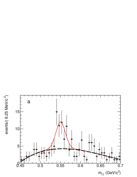
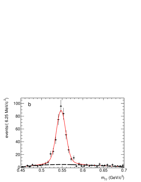
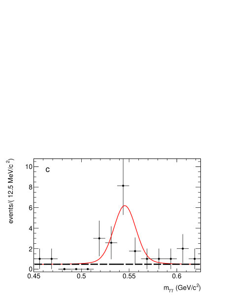
Figure 6: The two-photon invariant mass spectrum for data events (points with error bars) from the three $m_{\pi^{+}\pi^{-}\eta}$ intervals: $1.300-1.325$  ${\mathrm{\,Ge\kern-1.00006ptV\!/}c^{2}}$ (a), $1.500-1.525$ ${\mathrm{\,Ge\kern-1.00006ptV\!/}c^{2}}$ (b), and $3.4-3.5$ ${\mathrm{\,Ge\kern-1.00006ptV\!/}c^{2}}$ (c). The solid curve is the result of the fit described in the text. The dashed curve represents the fitted background.

IV Background subtraction

Figure 5 shows the distribution of the $\eta$-meson candidate invariant mass ($m_{\gamma\gamma}$) for Regions I and II. The invariant mass is calculated using the photon parameters returned by the 4C kinematic fit. The points with error bars represent data. The open histograms show the $m_{\gamma\gamma}$ distribution for signal simulated events. The shaded and hatched histograms show the expected contributions from background events peaking and nonpeaking at the $\eta$-meson mass, respectively. The peaking background arises from the processes $e^{+}e^{-}\rightarrow\pi^{+}\pi^{-}\pi^{0}\eta$, $e^{+}e^{-}\rightarrow K^{+}K^{-}\eta\gamma$, and $e^{+}e^{-}\rightarrow\pi^{+}\pi^{-}\pi^{0}\eta\gamma$.

\begin{overpic}[scale={0.5}]{Nevents_1.eps} \put(44.0,29.0){\includegraphics[scale={0.24}]{Nevents_2_3_1.eps}} \end{overpic}

Figure 7: The measured $\pi^{+}\pi^{-}\eta$ invariant mass spectrum (solid circles). The open circles show the same distribution for the peaking background obtained using MC simulation.

The number of signal events is determined from the fit to the $m_{\gamma\gamma}$ spectrum by a sum of signal and background distributions. The signal line shape is described by a double-Gaussian function, the parameters of which are obtained from MC simulation. The shape and the number of events for peaking background are calculated using MC simulation. In Region I, where simulation reproduces the $m_{\gamma\gamma}$ spectrum reasonably well (see Fig. 5a), the nonpeaking background shape is taken from MC simulation. In Region II (Fig. 5b), the background shape is assumed to be uniform in the $m_{\gamma\gamma}$ range from 0.45 to 0.65 ${\mathrm{\,Ge\kern-1.00006ptV\!/}c^{2}}$. The free fit parameters are the numbers of signal events and number of nonpeaking background events.

The fit is performed in the 59 $m_{\pi^{+}\pi^{-}\eta}$ bins listed in Table 1. The mass bin width is chosen to be 25 $\rm MeV/$$c^{2}$ below 2.0 ${\mathrm{\,Ge\kern-1.00006ptV\!/}c^{2}}$, and 50 (100) $\rm MeV/$$c^{2}$ in the range $2.0<m_{\pi^{+}\pi^{-}\eta}<3.1$ ($3.1<m_{\pi^{+}\pi^{-}\eta}<3.5$) ${\mathrm{\,Ge\kern-1.00006ptV\!/}c^{2}}$. Our measurement is restricted to the mass range $1.15<m_{\pi^{+}\pi^{-}\eta}<3.50$ ${\mathrm{\,Ge\kern-1.00006ptV\!/}c^{2}}$. Outside this range the signal to background ratio is too small to observe the signal. The fit results are shown in Fig. 6 for three representative $m_{\pi^{+}\pi^{-}\eta}$ bins. The fitted number of signal events as a function of the $\pi^{+}\pi^{-}\eta$ invariant mass is shown in Fig. 7 together with the $m_{\pi^{+}\pi^{-}\eta}$ spectrum for peaking background calculated using MC simulation. The total number of signal events is found to be $8065\pm 101$, while the numbers of peaking and nonpeaking background events are $239\pm 18$ and $3164\pm 64$, respectively.

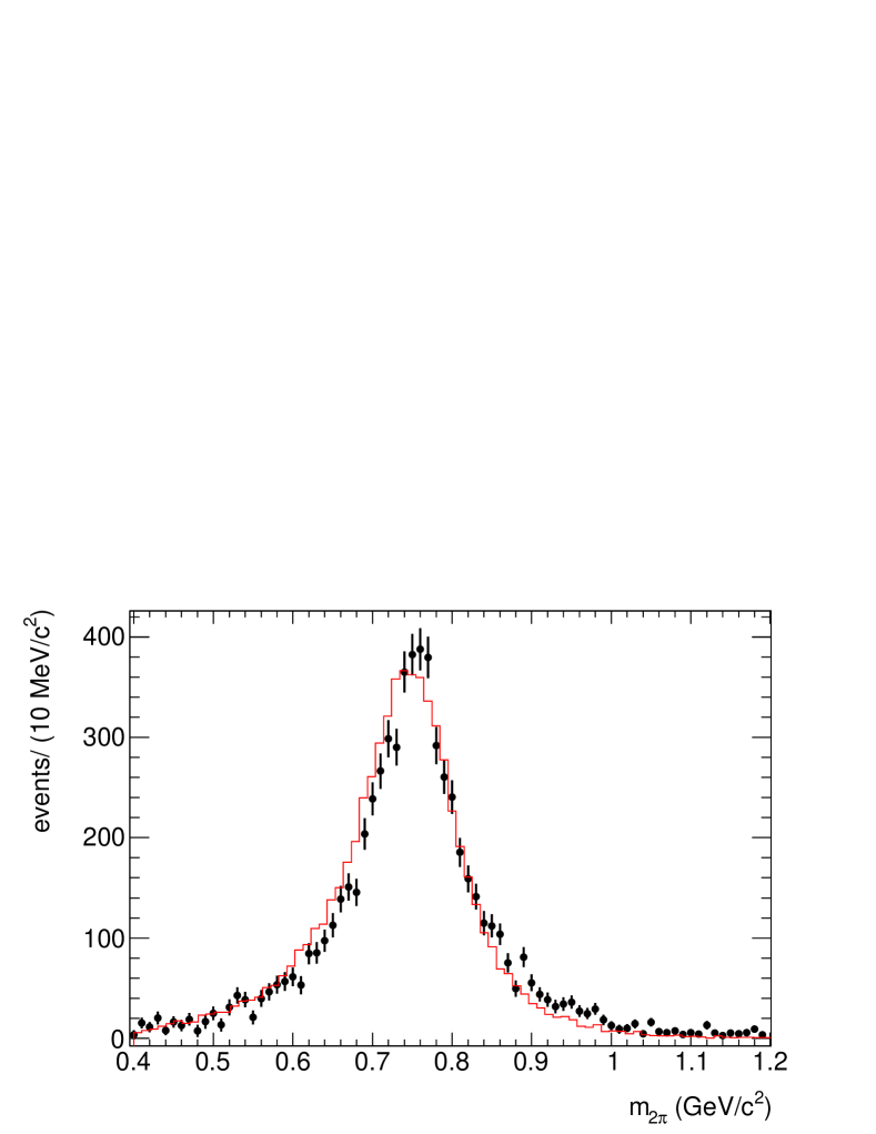
Figure 8: The two-pion invariant mass distribution for data (points with error bars) and simulated (histogram) events from the mass range $1.4<m_{\pi^{+}\pi^{-}\eta}<2.0$ ${\mathrm{\,Ge\kern-1.00006ptV\!/}c^{2}}$.

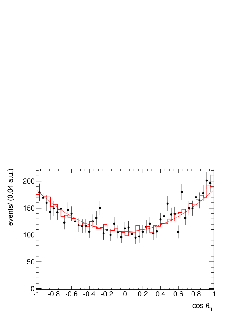
Figure 9: The $\cos{\theta_{\eta}}$ distribution for data (points with error bars) and simulated (histogram) events from the mass range $1.4<m_{\pi^{+}\pi^{-}\eta}<2.0$ ${\mathrm{\,Ge\kern-1.00006ptV\!/}c^{2}}$. The curve is the result of the fit described in the text.

A similar procedure of background subtraction is used to obtain the $\pi^{+}\pi^{-}$ invariant mass spectrum for data events in the range $1.4<m_{\pi^{+}\pi^{-}\eta}<2.0$ ${\mathrm{\,Ge\kern-1.00006ptV\!/}c^{2}}$. The spectrum is shown in Fig. 9 in comparison with the simulated signal spectrum. The simulation uses the model of the $\eta\rho(770)$ intermediate state. The observed difference between data and simulated spectra may be explained by the contribution of other intermediate states, for example $\eta\rho$(1450), and their interference with the dominant $\eta\rho(770)$ amplitude. This effect was observed previously in the SND experiment 2pieta_SND2014 .

Figure 9 shows the $\cos{\theta_{\eta}}$ distribution, where $\theta_{\eta}$ is the angle between the $\eta$ momentum in the $\pi^{+}\pi^{-}\eta$ rest frame and the ISR photon direction in the c.m. frame. In the $\eta\rho$ model this distribution is expected to be $(1+\cos^{2}{\theta_{\eta}})$. However the detection efficiency of the process under study depends on cos $\theta_{\eta}$ and data events are distributed as $(1+(0.73\pm 0.08)\cdot\cos^{2}{\theta_{\eta}})$ according to the fit shown by a curve in the figure. The detection efficiency is correctly reproduced in MC simulation and the distribution of reconstructed simulated events shown by a histogram in the figure is in reasonable agreement with data.

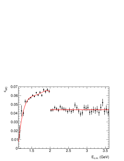
Figure 10: The detection efficiency $\varepsilon_{\text{MC}}$ obtained using MC simulation as a function of $E_{\rm c.m.}$. The lines are fits to a fourth-order polynomial for $E_{c.m.}<2$ GeV and to a constant for $E_{c.m.}>2$ GeV.

Table 1: Results of the $e^{+}e^{-}\rightarrow\pi^{+}\pi^{-}\eta$ reaction study: The c.m. energy range ($E_{\rm c.m.}$), number of selected events after $\pi^{+}\pi^{-}\eta$-mass-resolution correction ($N_{\rm corr}$), detection efficiency ($\varepsilon$), differential ISR luminosity ($L$), and measured cross section ($\sigma$). The systematic uncertainty on the cross section in different energy intervals is listed in Table 2.

$E_{\rm c.m.}$, GeV	$N_{\rm corr}$	$\varepsilon$, %	L, nb-1	$\sigma$, nb	$E_{\rm c.m.}$, GeV	$N_{\rm corr}$	$\varepsilon$, %	L, nb-1	$\sigma$, nb
1.150 - 1.175	$<$ 1 (90% C.L.)	1.36	1439.2	$<$ 0.05 (90% C.L.)	1.875 - 1.900	86 $\pm$ 12	6.17	2430.7	0.575 $\pm$ 0.081
1.175 - 1.20	$<$ 1 (90% C.L.)	2.12	1468.3	$<$ 0.03 (90% C.L.)	1.900 - 1.925	136 $\pm$ 14	6.19	2468.7	0.888 $\pm$ 0.092
1.20 - 1.225	9 $\pm$ 3	2.77	1498.0	0.231 $\pm$ 0.083	1.925 - 1.950	113 $\pm$ 13	6.18	2506.9	0.728 $\pm$ 0.086
1.225 - 1.250	2 $\pm$ 2	3.33	1528.0	0.058 $\pm$ 0.052	1.950 - 1.975	115 $\pm$ 13	6.15	2545.2	0.736 $\pm$ 0.085
1.250 - 1.275	13 $\pm$ 4	3.79	1558.6	0.228 $\pm$ 0.081	1.975 - 2.00	102 $\pm$ 12	6.08	2583.7	0.648 $\pm$ 0.081
1.275 - 1.300	38 $\pm$ 7	4.18	1589.6	0.583 $\pm$ 0.112	2.00 - 2.05	138 $\pm$ 12	4.14	5283.5	0.632 $\pm$ 0.057
1.300 - 1.325	32 $\pm$ 7	4.51	1621.1	0.444 $\pm$ 0.103	2.05 - 2.10	122 $\pm$ 11	4.14	5439.3	0.544 $\pm$ 0.050
1.325 - 1.350	72 $\pm$ 10	4.77	1652.9	0.914 $\pm$ 0.134	2.10 - 2.15	78 $\pm$ 9	4.14	5596.4	0.337 $\pm$ 0.039
1.350 - 1.375	107 $\pm$ 12	4.98	1685.1	1.280 $\pm$ 0.154	2.15 - 2.20	76 $\pm$ 9	4.14	5754.7	0.317 $\pm$ 0.038
1.375 - 1.40	144 $\pm$ 15	5.15	1717.7	1.628 $\pm$ 0.170	2.20 - 2.25	58 $\pm$ 8	4.14	5914.1	0.236 $\pm$ 0.033
1.400 - 1.425	195 $\pm$ 17	5.28	1750.7	2.103 $\pm$ 0.189	2.25 - 2.30	52 $\pm$ 7	4.14	6074.8	0.209 $\pm$ 0.031
1.425 - 1.450	281 $\pm$ 20	5.38	1784.0	2.920 $\pm$ 0.216	2.30 - 2.35	82 $\pm$ 9	4.14	6236.7	0.317 $\pm$ 0.036
1.450 - 1.475	357 $\pm$ 23	5.46	1817.6	3.582 $\pm$ 0.235	2.35 - 2.40	74 $\pm$ 9	4.14	6399.7	0.281 $\pm$ 0.033
1.475 - 1.500	380 $\pm$ 24	5.53	1851.6	3.699 $\pm$ 0.237	2.40 - 2.45	60 $\pm$ 8	4.14	6564.1	0.223 $\pm$ 0.030
1.500 - 1.525	419 $\pm$ 25	5.57	1885.9	3.970 $\pm$ 0.241	2.45 - 2.50	80 $\pm$ 9	4.14	6729.8	0.287 $\pm$ 0.032
1.525 - 1.550	436 $\pm$ 26	5.61	1920.5	4.035 $\pm$ 0.240	2.50 - 2.55	49 $\pm$ 7	4.14	6897.0	0.173 $\pm$ 0.026
1.550 - 1.575	424 $\pm$ 25	5.65	1955.3	3.826 $\pm$ 0.231	2.55 - 2.60	28 $\pm$ 5	4.14	7065.5	0.096 $\pm$ 0.019
1.575 - 1.600	394 $\pm$ 24	5.68	1990.5	3.476 $\pm$ 0.218	2.60 - 2.65	44 $\pm$ 7	4.14	7235.7	0.147 $\pm$ 0.023
1.600 - 1.625	355 $\pm$ 23	5.71	2025.9	3.065 $\pm$ 0.203	2.65 - 2.70	29 $\pm$ 5	4.14	7407.5	0.095 $\pm$ 0.018
1.625 - 1.650	324 $\pm$ 22	5.74	2061.6	2.732 $\pm$ 0.189	2.70 - 2.75	30 $\pm$ 5	4.14	7581.0	0.097 $\pm$ 0.018
1.650 - 1.675	307 $\pm$ 21	5.78	2097.5	2.528 $\pm$ 0.179	2.75 - 2.80	28 $\pm$ 5	4.14	7756.4	0.088 $\pm$ 0.017
1.675 - 1.700	269 $\pm$ 20	5.82	2133.7	2.161 $\pm$ 0.166	2.80 - 2.85	33 $\pm$ 6	4.14	7933.8	0.101 $\pm$ 0.018
1.700 - 1.725	285 $\pm$ 21	5.86	2170.1	2.233 $\pm$ 0.164	2.85 - 2.90	26 $\pm$ 5	4.14	8113.3	0.079 $\pm$ 0.015
1.725 - 1.750	278 $\pm$ 20	5.91	2206.7	2.130 $\pm$ 0.159	2.90 - 2.95	15 $\pm$ 4	4.14	8294.9	0.044 $\pm$ 0.012
1.750 - 1.775	280 $\pm$ 20	5.96	2243.6	2.091 $\pm$ 0.155	2.95 - 3.00	22 $\pm$ 5	4.14	8478.9	0.063 $\pm$ 0.014
1.775 - 1.800	270 $\pm$ 20	6.01	2280.6	1.965 $\pm$ 0.149	3.00 - 3.05	20 $\pm$ 5	4.14	8665.4	0.058 $\pm$ 0.014
1.800 - 1.825	282 $\pm$ 20	6.06	2317.9	2.005 $\pm$ 0.146	3.15 - 3.20	11 $\pm$ 4	4.14	9241.0	0.030 $\pm$ 0.010
1.825 - 1.850	182 $\pm$ 17	6.11	2355.3	1.262 $\pm$ 0.118	3.20 - 3.30	26 $\pm$ 5	4.14	19077	0.033 $\pm$ 0.007
1.850 - 1.875	145 $\pm$ 15	6.15	2392.9	0.987 $\pm$ 0.101	3.30 - 3.40	14 $\pm$ 4	4.14	19893	0.017 $\pm$ 0.005
1.875 - 1.900	86 $\pm$ 12	6.17	2430.7	0.575 $\pm$ 0.081	3.40 - 3.50	7 $\pm$ 3	4.14	20737	0.008 $\pm$ 0.003

V Detection efficiency and systematic uncertainties

Table 2: Summary of the efficiency corrections and systematic uncertainties on the measured cross section.

Source	Correction, %	Systematic
		uncertainty, %
Selection criteria		2.5
Background subtraction
$m_{\pi^{+}\pi^{-}\eta}<1.35$		9
$1.35<m_{\pi^{+}\pi^{-}\eta}<1.80$		2
$1.80<m_{\pi^{+}\pi^{-}\eta}<2.50$		5
$2.50<m_{\pi^{+}\pi^{-}\eta}<3.10$		10.5
$3.10<m_{\pi^{+}\pi^{-}\eta}<3.50$		11
Trigger and filters	-1.5	1.6
$\eta$ reconstruction	-2.0	1.0
ISR photon efficiency	-1.1	1.0
Track reconstruction	-1.1	1.0
Radiative correction		1.0
Luminosity		1.0
Total
$m_{\pi^{+}\pi^{-}\eta}<1.35$	-5.7	10
$1.35<m_{\pi^{+}\pi^{-}\eta}<1.80$	-5.7	4.5
$1.80<m_{\pi^{+}\pi^{-}\eta}<2.50$	-5.7	6.5
$2.50<m_{\pi^{+}\pi^{-}\eta}<3.10$	-5.7	11
$3.10<m_{\pi^{+}\pi^{-}\eta}<3.50$	-5.7	12

The corrected detection efficiency is defined as follows:

$$\varepsilon=\varepsilon_{\text{MC}}\prod_{i}(1+\delta_{i}),$$ (1)

where $\varepsilon_{\text{MC}}$ is the detection efficiency determined from MC simulation as the ratio of the true $\pi^{+}\pi^{-}\eta$ mass spectrum obtained after applying the selection criteria to the generated mass spectrum, and $\delta_{i}$ are the efficiency corrections, which take into account data-MC simulation differences in track and photon reconstruction, $\chi^{2}_{\rm 4C}$ distribution, etc. The detection efficiency $\varepsilon_{\text{MC}}$ as a function of $E_{c.m.}$ is shown in Fig. 10 where the lines are fits to a fourth-order polynomial for $E_{c.m.}<2$ GeV and to a constant for $E_{c.m.}>2$ GeV. A discontinuity in the efficiency at 2 GeV is caused by additional selection conditions used for Region II as mentioned in Sec. III.

To estimate efficiency corrections associated with the selection criteria, we loosen a criterion, perform the procedure of background subtraction described in the previous section, and calculate the ratio of the number of selected events in data and simulation. For example, the condition $\chi^{2}_{\rm 4C}<25(15)$ is loosened to $\chi^{2}_{\rm 4C}<300$. The efficiency correction is calculated as a relative difference between the data-MC simulation ratios calculated with the loosened and standard selection criteria. We do not observe any significant changes in data-MC simulation ratios due to variation of selection criteria and do not apply any corrections. The sum of the statistical uncertainties on the corrections for different selection criteria added in quadrature (2.5%) is taken as an estimate of the systematic uncertainty associated with the selection criteria.

To estimate the uncertainty related to the description of the nonpeaking background in the fit to the $m_{\gamma\gamma}$ spectrum, we repeat the fits using a quadratic background. The main source of peaking background is the process $e^{+}e^{-}\rightarrow\pi^{+}\pi^{-}\pi^{0}\eta$. Its contribution is calculated using the Jetset $q\bar{q}$ simulation normalized as described in Sec. III. In the normalization we assume that Jetset reproduces correctly the fraction of $\pi^{+}\pi^{-}\pi^{0}\eta$ events in the full sample of $q\bar{q}$ events satisfying our selection criteria. To estimate the systematic uncertainty associated with this assumption, we vary the fraction of $\pi^{+}\pi^{-}\pi^{0}\eta$ events by 50%. The obtained uncertainties associated with the nonpeaking and peaking backgrounds added in quadrature are listed in the section “Background subtraction” of Table 2.

We also study the quality of the simulation of the first-level trigger and background filters used in the primary event selection. The overlap of the samples of events passing different filters and trigger selections is used to estimate the filter and trigger efficiency. The latter is found to be reproduced by simulation, with accuracy better than $5\cdot 10^{-3}$. The correction due to data-MC simulation difference in the filter inefficiency is determined to be $(-1.5\pm 1.6)\%$.

To determine the efficiency correction for the data-MC simulation difference in $\eta$ candidate reconstruction, we use the results of the study of the $\pi^{0}$ reconstruction efficiency as a function of momentum described in Ref. pi0gg_BaBar . We assume that the $\eta\rightarrow\gamma\gamma$ efficiency is approximately equal to the $\pi^{0}\rightarrow\gamma\gamma$ efficiency at the same energy, and obtain the correction averaged over the $\eta$ momentum spectrum $\delta_{\eta}=(-2\pm 1)\%$. The correction is independent of the ${\pi^{+}\pi^{-}\eta}$ mass.

The ISR photon and charged-particle track reconstruction efficiencies are studied in Ref. 4pic_BaBar . The efficiency corrections and systematic uncertainties discussed in this section are summarized in Table 2.

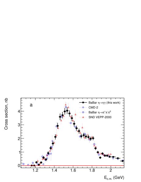
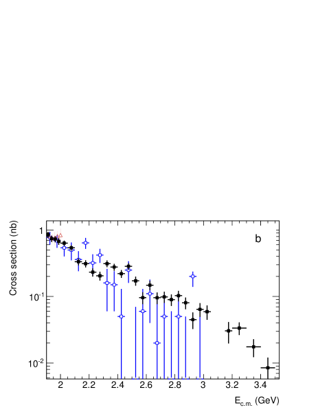
Figure 11: (color online) The $e^{+}e^{-}\rightarrow\pi^{+}\pi^{-}\eta$ cross section measured in this work (BABAR) in comparison with most precise previous measurements: CMD-2 CMD-2 , the independent BABAR(2007) BaBar2007 , SND 2pieta_SND2014 ) at $E_{\rm c.m.}<2.15$ GeV (a) and $E_{\rm c.m.}>1.9$ GeV (b).

VI The $\boldsymbol{e^{+}e^{-}\rightarrow\pi^{+}\pi^{-}\eta}$ cross section

From the measured $\pi^{+}\pi^{-}\eta$ mass spectrum, we calculate the Born cross section

$$\sigma(m)=\frac{(dN/dm)_{\text{corr}}}{dL/dm\cdot\varepsilon(m)\cdot R}~{},$$ (2)

where $m\equiv E_{\rm c.m.}/c^{2}$ is the invariant mass of the $\pi^{+}\pi^{-}\eta$ system, $(dN/dm)_{\text{corr}}$ is the $\pi^{+}\pi^{-}\eta$ mass spectrum after correction for the detector mass resolution (unfolding), $dL/dm$ is the so-called ISR differential luminosity 3piBaBar , $\varepsilon(m)$ is the detection efficiency, and $R$ is the radiative correction factor accounting for the Born $\pi^{+}\pi^{-}\eta$ mass spectrum distortion due to emission of several photons by the initial electron and positron. In our case the value of R is close to unity, and the theoretical uncertainty of $R$ does not exceed 1% NLO_ISR . The uncertainty of the total integrated luminosity collected by BABAR is less than 1% lumi .

The number of events in each bin $i$ ($N_{i}$) of the measured $\pi^{+}\pi^{-}\eta$ mass spectrum shown in Fig. 7 is related to the “true” number of events ($N_{\text{corr},i}$) as $N_{i}=\sum{A_{ij}N_{\text{corr},j}}$, where $A_{ij}$ is a migration matrix describing the probability for an event with “true” mass in the bin $j$ to contribute to bin $i$. The matrix $A_{ij}$ is determined from the signal MC simulation. For the 25 $\mathrm{\,Me\kern-1.00006ptV}$ bin width, diagonal elements of $A_{ij}$ are about 0.83, and next-to-diagonal elements are about 0.08. The inverse of the migration matrix is applied to the measured spectrum. The obtained $(dN/dm)_{\text{corr}}$ spectrum is used to calculate the cross section. Since the cross section does not contain narrow structures, the unfolded mass spectrum is close to the measured spectrum. The differences between their bin contents are found to be less than half the statistical uncertainty. But the correction leads to an increase in the errors (by 4-15%) and to correlations between the corrected numbers $N_{\text{corr},i}$. The neighbour to diagonal elements of the correlation matrix are about -20% and the elements after next about 2%.

The obtained $e^{+}e^{-}\rightarrow\pi^{+}\pi^{-}\eta$ cross section is listed in Table 1 and shown in Fig. 11 in comparison with the most precise previous measurements. The BABAR(2007) results used a different $\eta$ decay mode, and are independent. The energy region near the $J/\psi$ resonance (3.05–3.15 GeV) is excluded from the data listed in Table 1 and is discussed below. The nonresonant cross section at $E_{\rm c.m.}=m_{J/\psi}$ will be obtained in Sec. IX.

Our cross section results are in agreement with previous measurements, have comparable accuracy below 1.6 GeV and better accuracy above. In the energy range 3.0–3.5 GeV the cross sections are measured for the first time.

VII Fit to the $\boldsymbol{e^{+}e^{-}\rightarrow\pi^{+}\pi^{-}\eta}$ cross section

In the framework of the VMD model the $e^{+}e^{-}\rightarrow\pi^{+}\pi^{-}\eta$ cross section can be described by a coherent sum of contributions from isovector states V that decay into $\rho(770)\eta$ NNAChasov :

$$\sigma(s)=\frac{4\alpha^{2}}{3}\frac{1}{s\sqrt{s}}|F(s)|^{2}G(s),\,\,\,G(s)=\int_{4m_{\pi}^{2}}^{(\sqrt{s}-m_{\eta})^{2}}dq^{2}\frac{\sqrt{q^{2}}\Gamma_{\rho}(q^{2})p_{\eta}^{3}(s,q^{2})}{(q^{2}-m_{\rho}^{2})^{2}+(\sqrt{q^{2}}\Gamma_{\rho}(q^{2}))^{2}},$$ (3)

$$p_{\eta}^{2}=\frac{(s-m_{\eta}^{2}-q^{2})^{2}-4m_{\eta}^{2}q^{2}}{4s},\,\,\,\Gamma_{\rho}(q^{2})=\Gamma_{\rho}(m_{\rho}^{2})\frac{m_{\rho}^{2}}{q^{2}}\left(\frac{p^{2}_{\pi}(q^{2})}{p^{2}_{\pi}(m_{\rho}^{2})}\right)^{\frac{3}{2}},\,\,\,p^{2}_{\pi}(q^{2})=q^{2}/4-m_{\pi}^{2},$$ (4)

where $\sqrt{s}=E_{c.m.}$, $q$ is the $\pi^{+}\pi^{-}$ invariant mass, $m_{\eta}$ and $m_{\pi}$ are the $\eta$ meson and charged pion masses, $m_{\rho}$ and $\Gamma_{\rho}(m_{\rho}^{2})$ are the $\rho(770)$ mass and width, and

$$F(s)=\sum_{V}\frac{m_{V}^{2}g_{V}e^{i\phi_{V}}}{s-m_{V}^{2}+i\sqrt{s}\Gamma_{V}(s)},$$ (5)

where the sum is over all $\rho$ resonances and the complex parameter $g_{V}e^{i\phi_{V}}$ is the combination $g_{V\rho\eta}/g_{V\gamma}$ of the coupling constants describing the transitions $V\rightarrow\rho\eta$ and $V\rightarrow\gamma^{\star}$, respectively.

The VMD model [Eq.(3)] is used to fit our cross section data. The free fit parameters are $g_{V}$, and the masses and widths of the excited $\rho$-like states. The $\rho(770)$ mass and width are fixed at their Particle Data Group (PDG) values PDG . The phase $\phi_{\rho(770)}$ is set to zero. The coupling constants $g_{V\rho\eta}$ and $g_{V\gamma}$ are not expected to have sizable imaginary parts 2pieta_SND2014 . Therefore, we assume that $\phi_{V}$ for the excited states are 0 or $\pi$.

The models with one, two, and three excited states are tested. In Model 1, the cross section data are fitted in the energy range $E_{\rm c.m.}=1.2-1.70$ $\mathrm{\,Ge\kern-1.00006ptV}$ with two resonances, $\rho(770)$ and $\rho(1450)$. The model with $\phi_{\rho(1450)}=0$ fails to describe the data. The fit result with $\phi_{\rho(1450)}=\pi$ is shown in Fig. 12 by the long-dashed curve. The obtained fit parameters are listed in Table 3. It is seen that Model 1 cannot reproduce the structure in the cross section near 1.8 GeV.

Table 3: The coupling constants and resonance parameters obtained in the fits to the $e^{+}e^{-}\rightarrow\pi^{+}\pi^{-}\eta$ cross section data.

Parameter	Model 1	Model 2	Model 3	Model 4
$g_{\rho(770)}$, GeV-1	$1.1\pm 0.3$	$2.3\pm 0.3$	$1.8\pm 0.3$	$1.7\pm 0.3$
$g_{\rho(1450)}$, GeV-1	$0.49\pm 0.02$	$0.36\pm 0.05$	$0.44\pm 0.02$	$0.46\pm 0.03$
$g_{\rho(1700)}$, GeV-1	–	$0.044\pm 0.019$	$0.080\pm 0.012$	$0.016\pm 0.007$
$g_{\rho^{\prime\prime\prime}}$, GeV-1	–	–	–	$0.09\pm 0.02$
$m_{\rho(1450)}$, ${\mathrm{\,Ge\kern-1.00006ptV\!/}c^{2}}$	$1.487\pm 0.016$	$1.54\pm 0.01$	$1.50\pm 0.01$	$1.49\pm 0.01$
$m_{\rho(1700)}$, ${\mathrm{\,Ge\kern-1.00006ptV\!/}c^{2}}$	–	$1.76\pm 0.01$	$1.83\pm 0.01$	$1.83\pm 0.01$
$m_{\rho^{\prime\prime\prime}}$, ${\mathrm{\,Ge\kern-1.00006ptV\!/}c^{2}}$	–	–	–	$2.01\pm 0.04$
$\Gamma_{\rho(1450)}$, GeV	$0.33\pm 0.02$	$0.31\pm 0.03$	$0.28\pm 0.02$	$0.29\pm 0.02$
$\Gamma_{\rho(1700)}$, GeV	–	$0.16\pm 0.04$	$0.17\pm 0.02$	$0.08\pm 0.02$
$\Gamma_{\rho^{\prime\prime\prime}}$, GeV	–	–	–	$0.42\pm 0.09$
$\phi_{770,1450;...}$	0; $\pi$	0; $\pi;~{}\pi$	0; $\pi$; 0	0; $\pi$; 0; 0
$\chi^{2}$ per d.o.f.	14/16	35/21	19/21	28/26

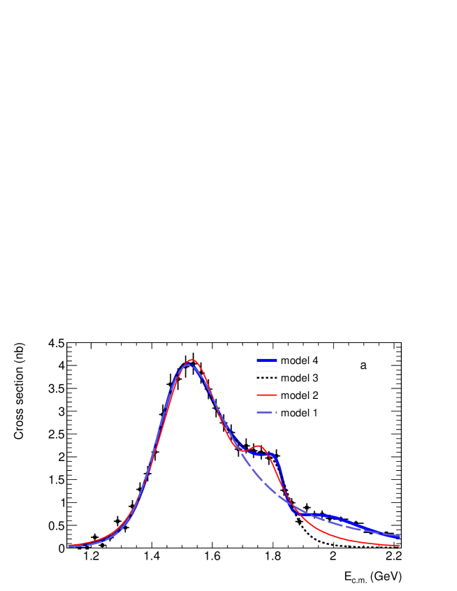
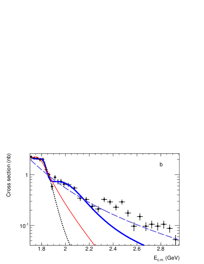
Figure 12: (color online) The measured $e^{+}e^{-}\rightarrow\pi^{+}\pi^{-}\eta$ cross section fitted with the four models described in the text.

In Models 2 and 3 we include an additional contribution from the $\rho(1700)$ resonance with phases $\phi_{\rho(1700)}$ = $\pi$ and 0, respectively. The fits are done in the range $E_{\rm c.m.}=$ 1.2–1.90 $\mathrm{\,Ge\kern-1.00006ptV}$. The fit results are shown in Fig. 12 and listed in Table 3. Both models describe the data below 1.90 $\mathrm{\,Ge\kern-1.00006ptV}$ reasonably well. Model 3 has better $\chi^{2}$ ($P(\chi^{2})=0.58$ instead of $0.03$ for Model 2). Above 1.90 $\mathrm{\,Ge\kern-1.00006ptV}$ the fit curves for both the models lie below the data.

Model 4 is Model 3 with a fourth resonance $\rho^{\prime\prime\prime}$ added. The phase $\phi_{\rho^{\prime\prime\prime}}$ is set to zero. The fitted energy range is extended up to 2.2 $\mathrm{\,Ge\kern-1.00006ptV}$. The fit result is shown in Fig. 12. The fitted resonance mass $m_{\rho^{\prime\prime\prime}}=2.01\pm 0.04$ GeV is between the masses of the $\rho(1900)$ and $\rho(2150)$ states listed in the PDG table PDG . The fitted value $g_{\rho}=1.7\pm 0.3$ GeV^-1 agrees with the VMD estimation of $1.57\pm 0.07$ GeV^-1 from the partial width $\rho(770)\rightarrow\eta\gamma$. It is seen that the model successfully describes the cross section data up to 2.3 $\mathrm{\,Ge\kern-1.00006ptV}$. Above $E_{\rm c.m.}=$ 2.3 $\mathrm{\,Ge\kern-1.00006ptV}$ Model 4 lies below the data, which could be explained by another resonance. Alternatively, the change of the cross section slope near 1.9 GeV may be interpreted without inclusion of a fourth resonance, as a threshold effect due to the opening of the nucleon-antinucleon production channel. Structures near the nucleon-antinucleon threshold are observed in the $e^{+}e^{-}\rightarrow 3(\pi^{+}\pi^{-})$ and $2(\pi^{+}\pi^{-}\pi^{0})$ cross sections threshold1 ; threshold2 as well as in the $\eta^{\prime}\pi^{+}\pi^{-}$ mass spectrum in the decay $J/\psi\rightarrow\gamma\eta^{\prime}\pi^{+}\pi^{-}$ threshold4 . A slope change near 1.9 GeV is seen in the $e^{+}e^{-}\rightarrow\pi^{+}\pi^{-}\pi^{+}\pi^{-}$ cross section threshold3 .

The fit is also performed with another parametrization. The parameters $g_{V}$ are replaced by the products

$$\Gamma(V\rightarrow e^{+}e^{-}){\cal B}(V\rightarrow\eta\pi^{+}\pi^{-})=\frac{\alpha^{2}}{9\pi}\frac{|g_{V}|^{2}m_{V}}{\Gamma_{V}}G(m_{V}^{2}).$$ (6)

From the fit in Model 3 we obtain:

$$\Gamma(\rho(1450)\rightarrow e^{+}e^{-}){\cal B}(\rho(1450)\rightarrow\eta\pi^{+}\pi^{-})=$$

$$(210\pm 24_{\text{stat}}\pm 10_{\text{syst}})\rm~{}eV$$

$$\Gamma(\rho(1700)\rightarrow e^{+}e^{-}){\cal B}(\rho(1700)\rightarrow\eta\pi^{+}\pi^{-})=$$

$$(84\pm 26_{\text{stat}}\pm 4_{\text{syst}})\rm~{}eV$$ (7)

The model uncertainties of these parameters estimated from the difference of fit results for Model 2, 3, and 4, are large, 20% for $\rho(1450)$ and 80% for $\rho(1700)$.

VIII Test of CVC

The CVC hypothesis and isospin symmetry allow the prediction of the $\pi^{-}\pi^{0}\eta$ mass spectrum and the branching fraction for the $\tau^{-}\rightarrow\pi^{-}\pi^{0}\eta\nu_{\tau}$ decay from data for the $e^{+}e^{-}\rightarrow\pi^{+}\pi^{-}\eta$ cross section CVC . The branching fraction can be calculated as:

$$\begin{gathered}\frac{{\cal B}(\tau^{-}\rightarrow\pi^{-}\pi^{0}\eta\nu_{\tau})}{{\cal B}(\tau^{-}\rightarrow e^{-}\bar{\nu_{e}}\nu_{\tau})}=\int_{(2m_{\pi}+m_{\eta})^{2}}^{m^{2}_{\tau}}dq^{2}\\ \sigma^{I=1}_{e^{+}e^{-}\rightarrow\pi^{+}\pi^{-}\eta}(q^{2})\frac{3|V_{ud}|^{2}S_{\text{EW}}}{2\pi\alpha^{2}}\frac{q^{2}}{m_{\tau}^{2}}(1-\frac{q^{2}}{m_{\tau}^{2}})^{2}(1+2\frac{q^{2}}{m_{\tau}^{2}}),\end{gathered}$$ (8)

where $q^{2}$ is the squared 4-momentum of the $\pi^{\pm}\pi^{0}\eta$ system, $|V_{ud}|$ is the Cabibbo-Kobayashi-Maskawa matrix element, and $S_{\text{EW}}=1.0194$ is a factor taking into account electroweak radiative corrections, and ${\cal B}(\tau^{-}\rightarrow e^{-}\bar{\nu_{e}}\nu_{\tau})$ = 17.83 $\pm$ 0.04% PDG .

We integrate Eq.(8) using the fit function for the cross section of model $\#4$ from the previous section and obtain

$$\begin{gathered}{\cal B}(\tau^{-}\rightarrow\pi^{-}\pi^{0}\eta\nu_{\tau})=(0.1616\pm 0.0026_{\text{stat}}\pm\\ 0.0080_{\text{syst}}\pm 0.0011_{\text{model}})\%=(0.162\pm 0.009)\%,\end{gathered}$$ (9)

where the first error is statistical, the second is systematic (see Table 2), and the third is model uncertainty.

The latter is estimated from the difference between the branching fraction values obtained with the cross section parametrization in Model 2 and Model 3 discussed in the previous section.

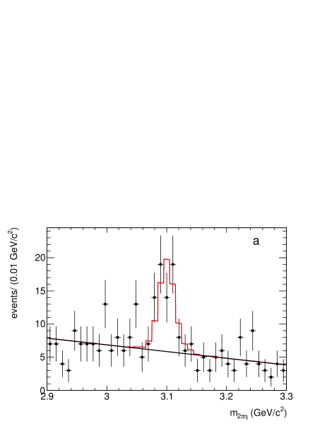
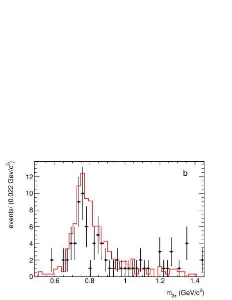
Figure 13: (a) The fit to the $\pi^{+}\pi^{-}\eta$ mass spectrum for data events from the $J/\psi$ region. (b) The $m_{\pi^{+}\pi^{-}}$ invariant mass distribution for data events with $3.05<m_{\pi^{+}\pi^{-}\eta}<3.15$ GeV/c² (points with error bars) and simulated signal events generated using the model with the $\rho(770)\eta$ intermediate state (histogram).

The calculation based on the previous BABAR measurement of the $\pi^{+}\pi^{-}\eta\rightarrow\pi^{+}\pi^{-}\pi^{+}\pi^{-}\pi^{0}$ final state BaBar2007 gives ${\cal B}(\tau^{\pm}\rightarrow\pi^{\pm}\pi^{0}\eta\nu_{\tau})=(0.1695\pm 0.0085_{\text{stat}}\pm 0.0136_{\text{syst}})\%$, compatible with the new result (9). The systematic uncertanties on the luminosity, radiative corrections, photon and track efficiencies are the same for the new and previous BABAR measurements. Combining the two BABAR values we obtain

$${\cal B}(\tau^{-}\rightarrow\pi^{-}\pi^{0}\eta\nu_{\tau})=(0.163\pm 0.008)\%,$$ (10)

which is in good agreement with, but more precise than, the estimate based on the SND $e^{+}e^{-}\rightarrow\pi^{+}\pi^{-}\eta$ measurement $(0.156\pm 0.011)\%$ 2pieta_SND2014 .

The PDG value of this branching fraction is ${\cal B}(\tau^{-}\rightarrow\pi^{-}\pi^{0}\eta\nu_{\tau})_{\rm exp}=(0.139\pm 0.010)\%$ PDG . The difference between the experimental result and our CVC-based calculation is $1.8\sigma$. The difference, about 15% of the branching fraction, is too large to be explained by isospin-breaking corrections. The quoted PDG value is based on the three measurements: $(0.135\pm 0.003\pm 0.007)\%$ by Belle Belle2009 , $(0.18\pm 0.04\pm 0.02)\%$ by ALEPH ALEPH1997 , and $(0.17\pm 0.02\pm 0.02)\%$ by CLEO CLEO1992 . Its error includes a scale factor of 1.4. The difference between our CVC prediction and the most precise measurement by Belle is $2.4\sigma$.

IX The $\boldsymbol{J/\psi\rightarrow\pi^{+}\pi^{-}\eta}$ decay

The $\pi^{+}\pi^{-}\eta$ mass spectrum for selected data events in the region near the $J/\psi$ is shown in Fig. 13(a). The spectrum is fitted by a sum of a function describing the $J/\psi$ line shape and a linear background function. The $J/\psi$ line shape is obtained using MC simulation. The fit yields $49\pm 9$ events of the decay $J/\psi\rightarrow\pi^{+}\pi^{-}\eta$.

From the fitted number of $J/\psi$ events we calculate the product NLO_ISR

$$\begin{gathered}\Gamma(J/\psi\rightarrow e^{+}e^{-}){\cal B}(J/\psi\rightarrow\pi^{+}\pi^{-}\eta)=\\ \frac{N_{J/\psi}m_{J/\psi}^{2}}{6\pi^{2}dL/dm(m_{J/\psi})\varepsilon(m_{J/\psi})}=\\ (2.34\pm 0.43_{\text{stat}}\pm 0.16_{\text{syst}})~{}\rm eV.\end{gathered}$$ (11)

Using the nominal value of the $J/\psi$ electron width $(5.55\pm 0.14)$ eV PDG we obtain the branching fraction

$${\cal B}(J/\psi\rightarrow\pi^{+}\pi^{-}\eta)=(4.2\pm 0.8)\times 10^{-4},$$ (12)

which has better precision than the current PDG value $(4.0\pm 1.7)\times 10^{-4}$ PDG .

Figure 13(b) shows the $m_{\pi^{+}\pi^{-}}$ invariant mass distributions for data events from the $J/\psi$ peak ($3.05<m_{\pi^{+}\pi^{-}\eta}<3.15$ GeV/c²) and simulated events. The simulation uses the model with the $\rho(770)\eta$ intermediate state. The difference between the $m_{\pi^{+}\pi^{-}}$ distributions for data and simulation is explained by the contribution of the isoscalar $\omega\eta$ intermediate state and its interference with the isovector amplitudes, where $\rho(770)\eta$ gives the main contribution J_psi_VP_DM2 ; J_psi_VP_MARK3 .

The G-parity of $\pi^{+}\pi^{-}\eta$ is +1, whereas G($J/\psi$) = -1. Therefore, this final state cannot be reached in strong-interaction (“direct”) decays. An allowed way for the decay is electromagnetic, $J/\psi\rightarrow\gamma^{*}\rightarrow\pi^{+}\pi^{-}\eta$. If this is the only way, the branching fraction has to fulfill:

$$\begin{gathered}{\cal B}(J/\psi\rightarrow\pi^{+}\pi^{-}\eta)/{\cal B}(J/\psi\rightarrow\mu^{+}\mu^{-})=\\ \sigma_{c}(e^{+}e^{-}\rightarrow\pi^{+}\pi^{-}\eta)/\sigma_{c}(e^{+}e^{-}\rightarrow\mu^{+}\mu^{-}),\end{gathered}$$ (13)

where $\sigma_{c}$ is the continuum cross section at $\sqrt{s}=m_{J/\psi}$ and $\sigma_{c}(e^{+}e^{-}\rightarrow\mu^{+}\mu^{-})=\frac{4\pi\alpha^{2}}{3m^{2}_{J/\psi}}$.

We obtain the continuum cross section for $\pi^{+}\pi^{-}\eta$ production by linear interpolation between four points near $m_{J/\psi}$, where two lie below 3.05 GeV/c² and two above 3.15 GeV/c²:

$$\sigma_{c}(e^{+}e^{-}\rightarrow\pi^{+}\pi^{-}\eta)=(47\pm 8_{\text{stat}}\pm 5_{\text{syst}})\mbox{pb}.$$ (14)

Inserting this result into Eq.(13) leads to

$$\begin{gathered}{\cal B}(J/\psi\rightarrow\pi^{+}\pi^{-}\eta)=\frac{3m^{2}_{J/\psi}}{4\pi\alpha^{2}}{\cal B}(J/\psi\rightarrow\mu^{+}\mu^{-})\\ \times\sigma_{c}(e^{+}e^{-}\rightarrow\pi^{+}\pi^{-}\eta)=(3.1\pm 0.6)\times 10^{-4}.\end{gathered}$$ (15)

This is smaller than the result in Eq.(12) by $(1.1\pm 1.0)\times 10^{-4}$. A second way to violate G-parity is the direct decay $J/\psi\rightarrow\omega\eta$ followed by the G-violating decay $\omega\rightarrow\pi^{+}\pi^{-}$. Our result confirms that there could be a sizeable contribution of the $\omega\eta$ intermediate state to the decay $J/\psi\rightarrow\pi^{+}\pi^{-}\eta$.

X Summary

In this paper we have studied the process $e^{+}e^{-}\rightarrow\pi^{+}\pi^{-}\eta\gamma$, in which the photon is emitted from the initial state. Using the ISR technique we have measured the $e^{+}e^{-}\rightarrow\pi^{+}\pi^{-}\eta$ cross section in the c.m. energy range from 1.15 up to 3.5 GeV. Our results are in agreement with previous measurements, including our own previous result in the independent $\eta\rightarrow\pi^{+}\pi^{-}\pi^{0}$ channel, and have comparable precision below 1.6 GeV and better precision above. In the energy range below 2.2 GeV the measured cross section is well described by the VMD model with four $\rho$-like resonances. Parameters of these resonances have been obtained.

Using the measured cross section and the CVC hypothesis, the branching fraction of the decay $\tau^{-}\rightarrow\eta\pi^{-}\pi^{0}\nu_{\tau}$ is determined to be ${\cal B}(\tau^{-}\rightarrow\pi^{-}\pi^{0}\eta\nu_{\tau})=(0.162\pm 0.009)$ %.

From the measured number of $e^{+}e^{-}\rightarrow J/\psi\gamma\rightarrow\pi^{+}\pi^{-}\eta\gamma$ events we have determined the product $\Gamma_{J/\Psi\rightarrow e^{-}e^{+}}{\cal B}_{J/\psi\rightarrow\pi^{+}\pi^{-}\eta}=2.34\pm 0.46$ eV, and the branching fraction ${\cal B}(J/\psi\rightarrow\pi^{+}\pi^{-}\eta)=(0.042\pm 0.008)\%$.

XI ACKNOWLEDGMENTS

We are grateful for the extraordinary contributions of our PEP-II colleagues in achieving the excellent luminosity and machine conditions that have made this work possible. The success of this project also relies critically on the expertise and dedication of the computing organizations that support BABAR. The collaborating institutions wish to thank SLAC for its support and the kind hospitality extended to them. This work is supported by the US Department of Energy and National Science Foundation, the Natural Sciences and Engineering Research Council (Canada), the Commissariat à l’Energie Atomique and Institut National de Physique Nucléaire et de Physique des Particules (France), the Bundesministerium für Bildung und Forschung and Deutsche Forschungsgemeinschaft (Germany), the Istituto Nazionale di Fisica Nucleare (Italy), the Foundation for Fundamental Research on Matter (The Netherlands), the Research Council of Norway, the Ministry of Education and Science of the Russian Federation, Ministerio de Economía y Competitividad (Spain), the Science and Technology Facilities Council (United Kingdom), and the Binational Science Foundation (U.S.-Israel). Individuals have received support from the Marie-Curie IEF program (European Union) and the A. P. Sloan Foundation (USA).

References

- (1) M. Benayoun et al., Mod. Phys. Lett. A 14, 2605 (1999).
- (2) A. B. Arbuzov et al., JHEP 9812, 009 (1998).
- (3) S. Binner, J. H. Kühn, and K. Melnikov, Phys. Lett. B 459, 279 (1999).
- (4) N. N. Achasov and V. A. Karnakov, JETP Lett. 39, 285 (1984).
- (5) V. A. Cherepanov and S. I. Eidelman, JETP Lett. 89, 9 (2009).
- (6) A. Cordier et al. (DM1 Collaboration), Nucl. Phys. B 172, 13 (1980).
- (7) V. P. Druzhinin et al. (ND Collaboration), Phys. Lett. B 174, 115 (1986).
- (8) A. Antonelli et al. (DM2 Collaboration), Phys. Lett. B 212, 133 (1988).
- (9) R. R. Akhmetshin et al. (CMD-2 Collaboration), Phys. Lett. B 489, 125 (2000).
- (10) M. N. Achasov et al. (SND Collaboration), JETP Lett. 92, 80 (2010).
- (11) V. M. Aulchenko et al. (SND Collaboration), Phys. Rev. D 91, 052013 (2015).
- (12) B. Aubert et al. (BABAR Collaboration), Phys. Rev. D. 76, 092005 (2007).
- (13) M. K. Volkov et al., Phys. Rev. C 89, 015202 (2014).
- (14) D. G. Dumm et al., Phys. Rev. D 86, 076009 (2012).
- (15) J. P. Lees et al. (BABAR Collaboration), Nucl. Instrum. Methods Phys. Res., Sect. A 726, 203 (2013).
- (16) B. Aubert et al. (BABAR Collaboration), Nucl. Instrum. Methods Phys. Res., Sect. A 479, 1 (2002).
- (17) B. Aubert et al. (BABAR Collaboration), Nucl. Instrum. and Meth. A 729, 615 (2013).
- (18) H. Czy and J. H. Khn, Eur. Phys. J. C 18, 497 (2001).
- (19) M. Caffo, H. Czy, E. Remiddi, Nuo. Cim. A 110, 515 (1997); Phys. Lett. B 327, 369 (1994).
- (20) E. Barberio, B. van Eijk and Z. Was, Comput. Phys. Commun. 66, 115 (1991).
- (21) S. Agostinelli et al. (Geant4 Collaboration), Nucl. Instrum. Methods Phys. Res., Sect. A 506, 250 (2003).
- (22) T. Sjöstrand, Comput. Phys. Commun. 82, 74 (1994).
- (23) J. P. Lees et al. (BABAR Collaboration), Phys. Rev. D 96, 092009 (2017).
- (24) B. Aubert et al. (BABAR Collaboration), Phys. Rev. D 77, 092002 (2008).
- (25) R. R. Akhmetshin et al., Phys. Lett. B 773, 150 (2017).
- (26) S. Jadach and Z. Was, Comput. Phys. Commun. 85, 453 (1995).
- (27) B. Aubert et al. (BABAR Collaboration), Phys. Rev. D 70, 072004 (2004).
- (28) B. Aubert et al. (BABAR Collaboration), Phys. Rev. D 80, 052002 (2009).
- (29) J. P. Lees et al. (BABAR Collaboration), Phys. Rev. D 85, 112009 (2012).
- (30) Y. S. Tsai, Phys. Rev. D 4, 2821 (1971).
- (31) R. R. Akhmetshin et al. (CMD-3 Collaboration), Phys. Lett. B 723, 82 (2013).
- (32) J. Haidenbauer, C. Hanhart, X. W. Kang and U. G. Meibner, Phys. Rev. D 92, 054032 (2015).
- (33) M. Ablikim et al. (BESIII Collaboration), Phys. Rev. Lett. 117, 042002 (2016).
- (34) J. P. Lees et al. (BABAR Collaboration), Phys. Rev. D 85, 112009 (2012).
- (35) C. Patrignani et al. (Particle Data Group), Chin. Phys. C 40, 100001 (2016).
- (36) K. Inami et al. (Belle Collaboration), Phys. Lett. B 672, 209 (2009).
- (37) D. Buskulic et al. (ALEPH Collaboration), Z. Phys. C 74, 263 (1997).
- (38) M. Artuso et al. (CLEO Collaboration), Phys. Rev. Lett. 69, 3278 (1992).
- (39) J. Jousset et al. (DM2 Collaboration), Phys. Rev. D 41, 5 (1990).
- (40) D. Coffman et al. (MARK-III Collaboration), Phys. Rev. D 38, 2695 (1988).