Spectroscopic diagnostics of the non-Maxwellian $\kappa$-distributions
using SDO/EVE observations of the 2012 March 7 X-class flare

Abstract

Spectroscopic observations made by the Extreme Ultraviolet Variability Experiment (EVE) on board the Solar Dynamics Observatory (SDO) during the 2012 March 7 X5.4-class flare (SOL2012-03-07T00:07) are analyzed for signatures of the non-Maxwellian $\kappa$-distributions. Observed spectra were averaged over 1 minute to increase photon statistics in weaker lines and the pre-flare spectrum was subtracted. Synthetic line intensities for the $\kappa$-distributions are calculated using the KAPPA database. We find strong departures ($\kappa$ $\lesssim$ 2) during the early and impulsive phases of the flare, with subsequent thermalization of the flare plasma during the gradual phase. If the temperatures are diagnosed from a single line ratio, the results are strongly dependent on the value of $\kappa$. For $\kappa$ = 2, we find temperatures about a factor of two higher than the commonly used Maxwellian ones. The non-Maxwellian effects could also cause the temperatures diagnosed from line ratios and from the ratio of GOES X-ray channels to be different. Multithermal analysis reveals the plasma to be strongly multithermal at all times with flat DEMs. For lower $\kappa$, the DEM_κ are shifted towards higher temperatures. The only parameter that is nearly independent of $\kappa$ is electron density, where we find log$(n_{\mathrm{e}}\,[\mathrm{cm}^{-3}])$ $\approx$ 11.5 almost independently of time. We conclude that the non-Maxwellian effects are important and should be taken into account when analyzing solar flare observations, including spectroscopic and imaging ones.

0000-0003-1308-7427]Jaroslav Dudík

1 Introduction

Solar flares (e.g. Fletcher et al., 2011) are brilliant yet transient manifestations of the solar magnetic activity. During flares, magnetic reconnection (e.g., Dungey, 153; Parker, 1957; Sweet, 1958; Priest & Forbes, 2000; Zweibel & Yamada, 2009; Aulanier et al., 2012; Janvier et al., 2013, 2015; Janvier, 2017) converts excess magnetic energy into other forms, such as thermal and kinetic energies (e.g., Emslie et al., 2012). A considerable portion of the released energy is converted into accelerated particles, producing enhanced high-energy tails, which are ubiquitously detected from flare free-free emission (e.g., Brown, 1971; Lin & Hudson, 1971; Holman et al., 2003; Saint-Hilaire et al., 2008; Krucker et al., 2008; Kašparová & Karlický, 2009; Veronig et al., 2010; Fletcher et al., 2011; Holman et al., 2011; Kontar et al., 2011; Zharkova et al., 2011; Oka et al., 2013, 2015; Simões et al., 2015; Battaglia & Kontar, 2013; Kuhar et al., 2016) and occur even in microflares (e.g., Hannah et al., 2008; Glesener et al., 2017; Wright et al., 2017). Generally, departures from the equilibrium Maxwellian distribution arise whenever particle acceleration is occurring, and the fundamental reason for existence of high-energy tails is the $\sim$$E^{-2}$ behavior of the electron collisional cross-section with the kinetic energy $E$ (Scudder & Olbert, 1979; Meyer-Vernet, 2007; Scudder & Karimabadi, 2013).

In this work, we study the influence of the high-energy tails on the intensities of the optically thin emission lines produced at flare temperatures. To quantify the departure from Maxwellian, we utilize the non-Maxwellian $\kappa$-distributions. These distributions are characterized by a power-law high-energy tail, and occur naturally in situations characterized by turbulence (Hasegawa et al., 1985; Laming & Lepri, 2007) which happen under flare conditions as well (Bian et al., 2014). Indeed, indications of the $\kappa$-distributions have been obtained from flare observations. Kašparová & Karlický (2009) showed that the bremsstrahlung spectra arising from flare plasma at coronal altitudes can be described by a $\kappa$-distribution. In their event, the flare chromospheric footpoint emission was occulted by the solar limb. Oka et al. (2013, 2015) showed that the $\kappa$-distributions provide a good description of the high-energy tail detected in above-the-loop-top sources, although a thermal Maxwellian component was also present.Indications of $\kappa$-distributions of ions with extremely non-Maxwellian values of $\kappa$ were also found by Jeffrey et al. (2016, 2017). These authors studied the emission arising in flare loop-top, ribbon, and hard X-ray footpoints, and showed that the emission line profiles are well-described by a $\kappa$-distribution.

Indications of the electron $\kappa$-distributions were also found in a transient coronal loop occurring in the same location as a previous B-class flare (Dudík et al., 2015). These authors analyzed the Fe XI–Fe XII emission line ratios observed by the Extreme-Ultraviolet Imaging Spectrometer (EIS, Culhane et al., 2007) onboard the Hinode satellite. The Fe XI–Fe XII line ratios were found to be strongly non-Maxwellian. Indications of the strongly non-Maxwellian distributions of both electrons and ions were also found in the transition region observations performed by the Interface Region Imaging Spectrograph (De Pontieu et al., 2014). Indications of the non-Maxwellian ions were found from the line profiles of Si IV and O IV, and electrons from the relative intensities of these lines (Dudík et al., 2017a). The values of $\kappa$ found from line profiles and line intensities were similar.

A review of the applications of the $\kappa$-distributions in solar physics can be found in Dudík et al. (2017c). Other astrophysical applications can be found e.g. in Pierrard & Lazar (2010) and Bykov et al. (2013). Finally we note that the $\kappa$-distributions can be used for description of plasma with multiple Maxwellian components (Hahn & Savin, 2015). Most of the additional Maxwellians are used to approximate the tail of the distribution, and their relative amplitudes decrease with increasing temperatures of these Maxwellians. In principle, a $\kappa$-distribution could thus represent a special case of multi-thermal plasma. Battaglia et al. (2015) used a differential emission measure (DEM) represented by a $\kappa$-distribution and fitted it to observations of a single-loop flare performed simultaneously by the Reuven-Ramaty High-Energy Solar Spectroscopic Imager (RHESSI, Lin et al., 2002) and the Atmospheric Imaging Assembly (AIA, Lemen et al., 2012; Boerner et al., 2012) onboard the Solar Dynamics Observatory (SDO, Pesnell et al., 2012). This analysis yielded $\kappa$ $\approx$ 4.

This paper is organized as follows. The flare selected for analysis (SOL2012-03-07T00:07) and its observations by the Extreme Ultraviolet Variability Experiment (EVE, Woods et al., 2012) onboard SDO are described in Sect. 2. The synthesis of non-Maxwellian optically thin spectra are detailed in Sect. 3. In Sect. 4, we describe the diagnostics of the flare plasma, including diagnostics of electron density (Sect. 4.1), temperature (Sect. 4.2), the parameter $\kappa$ (Sect. 4.3), differential emission measure (Sect. 4.4), as well as its influence on diagnostics of $\kappa$ (Sect. 4.5). A summary of the results is given in Sect. 5. Details on EVE lines and their blends are given in Appendix A.

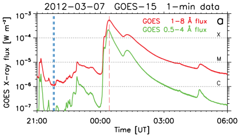
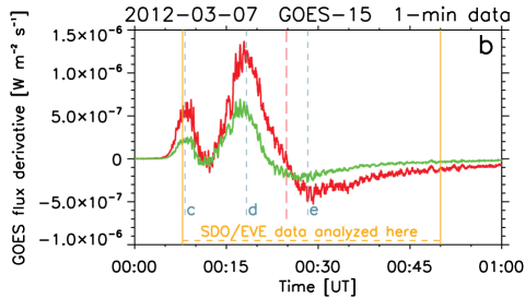
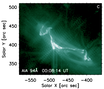
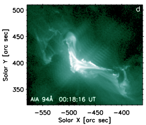
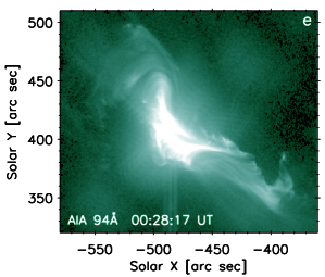
Figure 1: Context observations of the X5.4-class flare of 2012 March 7 from GOES-15 and SDO/AIA. (a)–(b): GOES-15 X-ray flux and its derivative, respectively. Red and blue vertical dashed lines indicate the time of the flare peak and the interval where the pre-flare spectrum was selected, respectively. (c)–(e): SDO/AIA imaging observations (log scaled) of the flare in the 94 Å channel dominated by Fe XVIII. The times shown are indicated in panel (b) by green vertical dashed lines.

2 Observations

2.1 The X5.4-class flare of 2012 March 07

The X5.4-class flare of 2012 March 07 (SOL2012-03-07T00:07) is the fourth largest flare of the current Solar cycle 24, according to the X-ray Flare Dataset. It occurred in the Active region NOAA 11429, which was a well-known flaring region studied by many authors (e.g., Doschek et al., 2013; Simões et al., 2013; Schrijver & Higgins, 2015; Brown et al., 2016; Harra et al., 2016; Polito et al., 2017; Dudík et al., 2017b). On 2012 March 07, the AR 11429 possessed a $\delta$-spot in anti-Hale configuration, a situation prone to strong flaring (Chintzoglou et al., 2015). The X5.4-class flare was followed in its gradual phase by another X1.3-class flare about an hour later (Fig. 1). These two flares were sources of two super-fast CMEs (Chintzoglou et al., 2015).

Spectroscopic analysis of the Hinode/EIS observations of confined flares occurring prior to the eruptive ones were performed by Syntelis et al. (2016). Formation of the two erupting flux ropes during the confined flares and the pre-eruptive magnetic geometry were studied by Chintzoglou et al. (2015). The hydrogen Lyman series and C III emission of the X-class flare from SDO/EVE was examined by Brown et al. (2016). Other aspects of the X-class flares, such as the $\gamma$-ray and proton observations, as well as the CMEs and their propagation were studied by Ajello et al. (2014), Kouloumvakos et al. (2016) and Patsourakos et al. (2016). The flare was not observed by RHESSI, which started its observations only after 02:05 UT.

The X-ray flux and its derivative during the X5.4-class flare are shown in Fig. 1, panels (a) and (b), respectively. A strong rise of the X-ray flux started at about 00:06 UT on 2012 March 07, followed by the impulsive phase. The flare reached its maximum at about 00:25 UT (red dashed line in Fig. 1a) and progressed to the gradual phase. The morphology of the flare is shown in panels (c) to (e) of Fig. 1. There, the imaging observations performed by the SDO/AIA instrument (Lemen et al., 2012; Boerner et al., 2012) in its 94 Å channel are shown. The 94 Å channel is dominated by Fe XVIII 93.93 Å emission under flaring conditions (O’Dwyer et al., 2010; Petkaki et al., 2012). The morphology at the flare onset (panel c) is suggestive of a sheared magnetic configuration (c.f., Chintzoglou et al., 2015) with brightenings close to the polarity inversion line. Subsequently, the flare develops into an arcade of flare loops, growing both laterally along the polarity inversion line as well as across it, with decreasing magnetic shear, in agreement with the Standard solar flare model in 3D (Aulanier et al., 2012; Janvier et al., 2013, 2015). The flare is very bright and thus most of the AIA pass-bands are saturated even at lower exposure times.

2.2 SDO/EVE observations of the flare

The Extreme Ultraviolet Variability Experiment (EVE, Woods et al., 2012) on board the Solar Dynamics Observatory (SDO, Pesnell et al., 2012) is a collection of instruments for measuring the solar EUV irradiance from 1 to 1050 Å with spectral resolution of $\approx$1 Å at a cadence of about 10 s. For our purposes, we used the data obtained by the Multiple EUV Grating Spectrographs A and B. The MEGS-A was a routinely operating (until 2014 May 26) grazing-incidence, off-Rowland circle spectrograph measuring at 50–370 Å. The MEGS-B is a normal-incidence, dual-pass spectrograph operating at wavelengths above 350Å and up to 1050 Å. The MEGS-B instrument suffered degradation limiting its operations.

Both MEGS-A and B instruments observed the 2012 March 07 flare at full cadence of 10 s throughout the rise, impulsive, peak, and gradual phases of the flare. Here, we analyze both MEGS-A and B observations made during 00:08 – 00:50 UT. During this interval, the flare lines, including the weaker lines required for diagnostics (Sect. 4) are well-observed. This time interval captures nearly the entirety of the flare from the early phase up to the beginning of its gradual phase (c.f., Fig. 1b).

The EVE observations of the flare were analyzed by Del Zanna & Woods (2013). There, example spectra during the pre-flare, impulsive, peak, and gradual phases are shown together with the lightcurves of the selected strong lines, especially Fe lines from various ionization stages (Fe IX–Fe XXIII; see also Harra et al., 2016). Diagnostics of temperature, electron density, and emission measure were also performed and discussed by Del Zanna & Woods (2013). The low EVE spectral resolution of $\approx$1 Å means that most of the lines observed are blended. The known and unknown blends, their wavelengths, contribution to the intensity of the main line, behavior with temperature and flare evolution were also discussed by Del Zanna & Woods (2013).

3 Non-Maxwellian line intensity calculations

Here, we re-visit the EVE flare observations to perform non-Maxwellian diagnostics of the plasma, as well as to analyze the influence of the departures from the Maxwellian on the diagnosed temperature $T$ and electron density $n_{\mathrm{e}}$. To do that, we use the non-Maxwellian $\kappa$-distributions (e.g., Olbert, 1968; Vasyliunas, 1968a, b; Owocki & Scudder, 1983; Livadiotis, 2015; Dzifčáková et al., 2015)

$$f_{\kappa}(E)dE=A_{\kappa}\frac{2}{\sqrt{\pi}\left(k_{\mathrm{B}}T_{\kappa}\right)^{3/2}}\frac{E^{1/2}dE}{\left(1+\frac{E}{(\kappa-3/2)k_{\mathrm{B}}T_{\kappa}}\right)^{\kappa+1}}\,,$$ (1)

which allows for modeling of the effect of the high-energy tails by using only one extra free parameter, $\kappa$. Maxwellian distribution is recovered for $\kappa$ $\to$ $\infty$, while extreme non-Maxwellian situations occur for $\kappa$ $\to$ 3/2. In Eq. (1), $E$ is the electron kinetic energy, $k_{\mathrm{B}}$ = 1.38 $\times$10^-16 erg K^-1 is the Boltzmann constant, and $A_{\kappa}$ = $\Gamma(\kappa+1)/(\Gamma(\kappa-1/2)(\kappa-3/2)^{3/2}$ is the normalization constant.

The $\kappa$-distribution is characterized by a near-Maxwellian core with temperature $T_{\mathrm{C}}$ = $(\kappa-3/2)/\kappa$ (Oka et al., 2013, Section 2 and Figure 1 therein) and a power-law high-energy tail with the power-law index of $\kappa+1/2$ (Eq. 1). In terms of the power-law index of bremsstrahlung radiation (see also Dudík et al., 2012) routinely observed in X-rays in case of a thin-target source, $\gamma_{\mathrm{thin}}$ = $\delta$+1 = $\delta^{\prime}$+1/2, where $\gamma_{\mathrm{thin}}$ is the power-law index of the photon flux spectrum, and $\delta$ and $\delta^{\prime}$ are the power-law indices of electron energy flux and energy distributions, respectively (c.f., Brown, 1971; Tandberg-Hanssen & Emslie, 1988). For a $\kappa$-distribution, $\delta^{\prime}$ = $\kappa$+1/2 (Equation 1). This means that $\delta$ = $\kappa$ and $\gamma_{\mathrm{thin}}$ = $\kappa+1$ (see Dudík et al., 2012, 2017c).

The behavior of the emission lines with $\kappa$ is more complicated. The intensity $I_{ji}$ of a spectral line arising from plasma along a line of sight $l$ is given by (cf., Mason & Monsignori Fossi, 1994; Phillips et al., 2008)

$$I_{ji}=\int A_{X}G_{X,ji}(T,n_{\mathrm{e}},\kappa)n_{\mathrm{e}}n_{\mathrm{H}}\mathrm{d}l\,,$$ (2)

where $G_{X,ji}(T,n_{\mathrm{e}},\kappa)$ is the line contribution function

$$G_{X,ji}(T,n_{\mathrm{e}},\kappa)=\frac{hc}{\lambda_{ji}}\frac{A_{ji}}{n_{\mathrm{e}}}\frac{n(X_{j}^{+k})}{n(X^{+k})}\frac{n(X^{+k})}{n(X)}\,.$$ (3)

In these equations, $j$ and $i$ stand for the upper and lower level corresponding to the radiative transition arising from the $X^{+k}$ ion of the element $X$ of abundance $A(X)$. The corresponding wavelength is denoted as $\lambda_{ji}$ and the Einstein coefficient as $A_{ji}$. The fractions $n(X_{j}^{+k})/n(X^{+k})$ and $n(X^{+k})/n(X)$ denote the density of excited fraction of the ion $X^{+k}$ and the relative abundance of this ion, respectively. These ratios are both a function of $\kappa$ due to the dependence of individual excitation, deexcitation, ionization, and recombination rates on $\kappa$ (e.g., Dzifčáková, 1992, 2002; Dzifčáková & Dudík, 2013; Dudík et al., 2014b; Dzifčáková et al., 2015). These rates are integral quantities of the respective cross-sections over the electron energy distribution. Thus, collisional processes across many orders of electron energies are involved in the line intensity calculation. The rates of all processes show significant departures from the Maxwellian with decreasing $\kappa$. For small $\kappa$, the ionization and ionization rates are increased by orders of magnitude at low $T$ (e.g., Dzifčáková, 2006; Dzifčáková & Dudík, 2013; Dudík et al., 2014a) compared to Maxwellian. The recombination rates are increased by a factor of about two for $\kappa$ = 2, however, the peak of the dielectronic recombination can be shifted to higher $T$.

In inhomogeneous situations involving many emitting structures along a given line of sight, or in case of EVE indeed the full Sun, the expression (2) is usually recast as

$$I_{ji}=\int A_{X}G_{X,ji}(T,n_{\mathrm{e}},\kappa)\mathrm{DEM}_{\kappa}(T)\mathrm{d}T\,,$$ (4)

where the quantity DEM${}_{\kappa}(T)=n_{\mathrm{e}}n_{\mathrm{H}}\mathrm{d}l/\mathrm{d}T$ is the differential emission measure, i.e., the contribution to total emission measure along the line of sight from plasma at a given $T$. Here, the subscript $\kappa$ indicates that the DEM can be a function of $\kappa$ (c.f., Mackovjak et al., 2014; Dudík et al., 2015).

Spectral synthesis and calculation of line intensities for the $\kappa$-distributions were performed using the KAPPA database (Dzifčáková et al., 2015). KAPPA is based on the CHIANTI database and software, version 7.1 (Dere et al., 1997; Landi et al., 2013). We note that CHIANTI has been updated to version 8 (Del Zanna et al., 2015); however, the atomic data for the Fe XVIII–Fe XXIII that we use here are the same in CHIANTI versions 7.1 and 8. The main atomic data used for level population were obtained by Witthoeft et al. (2006) and Del Zanna (2006) for Fe XVIII, (Gu, 2003) and Landi & Gu (2006) for Fe XIX, Witthoeft et al. (2007) for Fe XX, Badnell & Griffin (2001) and Landi & Gu (2006) for Fe XXI, Badnell et al. (2001) and Landi & Gu (2006) for Fe XXII, and Chidichimo et al. (2005) and Del Zanna et al. (2005) for Fe XXIII. The former references listed stand for the effective collision strengths, while the latter for the $A$-values. Finally, for Fe XXIV, we use the atomic data of Berrington & Tully (1997) and Whiteford et al. (2002) available within CHIANTI v7.1 and KAPPA databases. These are different from the atomic data available within CHIANTI v8, which relies on Whiteford et al. (2001) and Badnell (2011). The different atomic datasets result in very similar intensities; the difference for typical flare conditions is about 14% for the 192.03 Å line used here.

Finally, atomic data for ionization and recombination used for ionization equilibrium calculations (Dzifčáková & Dudík, 2013) were taken from the works of Dere (2007) and Dere et al. (2009) for ionization, and Badnell et al. (2003), Colgan et al. (2003), Colgan et al. (2004), Mitnik & Badnell (2004), Badnell (2006), Altun et al. (2005, 2006, 2007), Zatsarinny et al. (2005a), Zatsarinny et al. (2005b), Zatsarinny et al. (2006), Bautista & Badnell (2007), and Nikolić et al. (2010) for recombination.

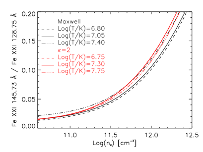
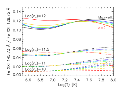
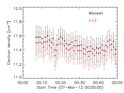
Figure 2: Electron density diagnostics. Top and middle: Theoretical dependence of the Fe XXI 145.73 Å / 128.75 Å ratio on electron density as a function of $T$ and $\kappa$. Colors stand for different $\kappa$, while individual linestyles denote dependence on $T$ (top) or $n_{\mathrm{e}}$ (middle). Bottom: Diagnosed values of $n_{\mathrm{e}}$ and their uncertainties as a function of time, assuming either a Maxwellian (black) or $\kappa$ = 2 (red) distribution.

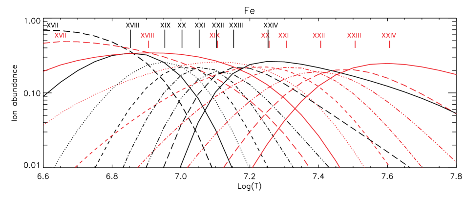
Figure 3: Relative ion abundances in ionization equilibrium as a function of $T$ plotted for the Maxwellian distribution (black) and $\kappa$ = 2 (red color). Loci of the peaks of the abundance of individual ions are shown by vertical lines with labels.

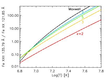
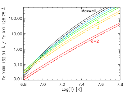
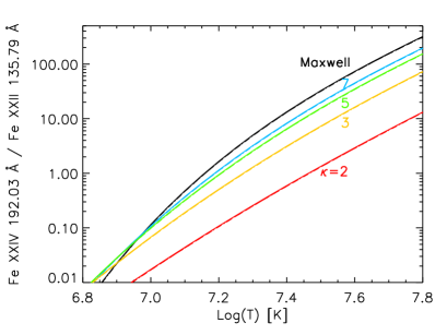
Figure 4: Temperature diagnostics from line intensity ratios as a function of $\kappa$. Colors denote individual values of $\kappa$. Individual linestyles denote different electron densities. Full and dashed lines stand for log($n_{\mathrm{e}}$ [cm^-3]) = 11 and 12, respectively. Note the logarithmic scaling of the line intensity ratio axes.

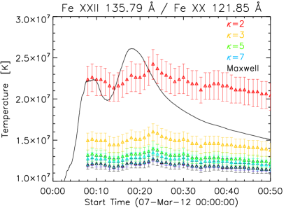
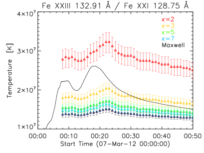
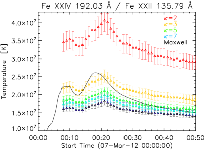
Figure 5: Temperatures and their evolution diagnosed using the individual theoretical ratios from Fig. 4. Colors denote the value of $\kappa$ as indicated. The thin black lines stand for the temperature derived from the ratio of the two GOES channels.

4 Plasma diagnostics

We now proceed to diagnose the basic plasma parameters: Electron density $n_{\mathrm{e}}$, electron temperature $T$, the $\kappa$ index, as well as the differential emission measure. To do this, line intensity ratios are used for diagnostics of $n_{\mathrm{e}}$, $T$, and $\kappa$, while lines spanning many ionization stages are used to diagnose the flare DEM${}_{\kappa}(T)$.

Because of the low spectral resolution of EVE ($\approx$1 Å, Woods et al., 2012) and the typical FWHM of flare lines is about 0.75 Å, most of the lines are blended (Del Zanna & Woods, 2013). Known blends from Fe flare lines were added to theoretical intensity calculations. To estimate the contribution of non-Fe unresolvable blends, we re-calculated the intensities of lines of interest including all contributions included in the CHIANTI v7.1 and KAPPA databases. These contributions were calculated as a function of temperature and then folded over the DEM${}_{\kappa}(T)$ derived from the flare (Sect. 4.4). These re-calculated contribution functions involving non-Fe were however not used for diagnostics, because of possible difficulties with anomalous abundances during flares (see Doschek et al., 2015; Doschek & Warren, 2016). Subsequently, lines that were strongly blended by non-Fe lines were excluded from diagnostics. Weaker significant blends, as well as all other details on individual lines used for different types of diagnostics are discussed in Appendix A.

To enhance the signal-to-noise ratio in weaker lines, we performed averaging over 1 minute intervals. Furthermore, from each 1-minute averaged spectrum, we subtracted the pre-flare spectrum, which was obtained as an average over 3 minutes during the pre-flare period at 21:46 – 21:49 UT, i.e., when the GOES X-ray signal was low, unperturbed by other flaring activity. These times are noted by blue dashed lines in Fig. 1a. We note that subtracting the pre-flare spectrum is a standard practice for analysis of EVE spectra (e.g., Milligan et al., 2012; Del Zanna & Woods, 2013). This greatly helps to remove the blends from coronal and low-temperature lines. We also note that the coronal lines do not change strongly ($\lessapprox$20%) during the flare, see Fig. 1 in Del Zanna & Woods (2013).

Each subtracted spectrum was fitted using the XCFIT procedure available within SolarSoft, assuming a constant pseudo-continuum and Gaussian functions for each visible line feature including resolved blends within line wings. Details on the fitting of each line are also given in Appendix A. Finally, the uncertainties of the measured intensities include the photon noise uncertainty added in quadrature with the EVE calibration uncertainty, which is about 20% (Woods et al., 2012). For the weakest lines used here, the overall uncertainty can reach $\approx$40%.

4.1 Electron density diagnostics

The electron density $n_{\mathrm{e}}$ is not a parameter of the distribution in Eq. (1) in the same manner as $T$ or $\kappa$. Thus, it can and should be diagnosed prior and separately from $T$ and $\kappa$ (Dzifčáková & Kulinová, 2010; Dudík et al., 2014b, 2015). Here, we use the well-known density-sensitive line ratio of Fe XXI 145.73 Å / 128.75 Å (Mason et al., 1979, 1984; Milligan et al., 2012; Del Zanna & Woods, 2013) which is density-sensitive above $\approx$10¹¹ cm^-3, i.e., in conditions corresponding to large flares (Milligan et al., 2012). The sensitivity to $n_{\mathrm{e}}$ arises due to the presence of metastable levels within Fe XXI, whose population is not strongly sensitive to either $T$ or $\kappa$.

The theoretical line intensity ratio is shown in Fig. 2 top as a function of $n_{\mathrm{e}}$. There, black and red colors denote Maxwellian and $\kappa$ = 2 distributions, respectively, i.e., the extreme values of the parameter $\kappa$ considered here. Individual linestyles denote different temperatures. The full lines correspond to the peak of the ionization equilibrium for a given $\kappa$, while the dashed and dash-dotted lines correspond to ion abundance being 10^-2 of the ion abundance peak. Thus, they denote the temperature interval where the ion is dominantly formed (see Fig. 3). Further quantification of the dependence of the Fe XXI 145.73 Å / 128.75 Å ratio on $T$ and $\kappa$ is provided in Fig. 2 middle. It is obvious that the line intensity ratio is not strongly sensitive to either $T$ or $\kappa$.

Both Fe XXI 128.75 Å and 145.73 Å lines are well observed by EVE (Milligan et al., 2012; Del Zanna & Woods, 2013). However, due to the relatively large uncertainty of the line intensities, the diagnosed electron densities (Fig. 2, bottom) have an uncertainty of about 0.3 in log$(n_{\mathrm{e}}\,[\mathrm{cm}^{-3}])$. The densities diagnosed under the assumption of a Maxwellian or a $\kappa$-distribution are similar, about log$(n_{\mathrm{e}}\,[\mathrm{cm}^{-3}])$ $\approx$ 11.5; with the densities diagnosed for $\kappa$ = 2 being $\approx$0.15 dex smaller than those for the Maxwellian distribution. We note that this is a typical feature of the non-Maxwellian density diagnostics (see Dzifčáková & Kulinová, 2010; Dudík et al., 2014b, 2015).

The observed densities do not evolve significantly during the flare, apart from perhaps a modest decrease with time. This decrease is however much smaller than the uncertainties of the diagnosed densities. We note that the observed density and its evolution is an average over the flare, since EVE is a full-Sun spectrometer. The absence of significant evolution is thus likely due to appearance of newer and newer flare loops. We also note that hydrodynamic models reflecting the overall evolution of many flare loops have been constructed, yielding similar absence of strong density evolution lasting for thousands of seconds (e.g., Sun et al., 2013; Polito et al., 2016). In this respect, the reported density evolution is not unusual as it likely reflects a continuing energy release in the flare.

4.2 Electron temperature diagnostics

As mentioned in Sect. 3, both $T$ and $\kappa$ are free parameters of the distribution. Thus, diagnostics of temperature has to be done either simultaneously with $\kappa$ (Sect. 4.3), or under an assumption of a constant $\kappa$. Since the latter is instructive in terms of influence of the $\kappa$-distributions on the observed spectra, we discuss this method first.

Under an assumption of constant $\kappa$, the diagnosed temperatures will necessarily depend on the assumed value of $\kappa$. This behavior comes primarily from the dependence of the ionization equilibrium on $\kappa$ (Fig. 3): The peaks of the relative ion abundance are wider and shifted to higher $T$ for lower $\kappa$ (Dzifčáková & Dudík, 2013). Thus, the temperatures diagnosed for smaller $\kappa$ will be higher.

To perform this diagnostics of $T$, we use the same three line intensity ratios as Del Zanna & Woods (2013). These line ratios involve a pair of ions from different ionization stages, where the difference in ion charge is 2. This offers large sensitivity to $T$. The lines used are Fe XX 121.85 Å, Fe XXI 128.75 Å, Fe XXII 135.79 Å, Fe XXIII 132.91 Å, and Fe XXIV 192.03 Å (see Appendix A for details). The theoretical temperature-diagnostic curves for different $\kappa$ are shown in Fig. 4. With progressively smaller $\kappa$, the curves are shifted to larger $T$ and are less steep, as expected.

The temperatures diagnosed using an assumption of constant $\kappa$ and the observed line ratios of Fe XXII 135.79 Å / Fe XX 121.85 Å, Fe XXIII 132.91 Å / Fe XXI 128.75 Å, and Fe XXIV 192.03 Å / Fe XXII 135.79 Å are shown in Fig. 5 together with their respective uncertainties. The diagnosed temperatures indeed depend on the assumed value of $\kappa$. Progressively larger $T$ are obtained for smaller $\kappa$, with the $T_{\kappa=2}$ being about a factor of two higher than the $T_{\mathrm{Maxw}}$. This illustrates the importance of non-Maxwellian effects for diagnostics of temperature.

For comparison, the temperatures derived from the ratio of the two GOES channels (assuming Maxwellian) are shown as thin solid line. In accordance with the results of Del Zanna & Woods (2013), it is seen that the GOES temperatures are discrepant from the Maxwellian temperatures by a factor of up to about two. That the $\kappa$-distributions yield higher temperatures for small $\kappa$ could hint at a possible resolution of this discrepancy. We however note that the $T_{\mathrm{GOES}}$ are likely a function of $\kappa$ as well, since at least the slope of the free-free continuum within the GOES pass-bands is a function of $\kappa$ at flare temperatures (see Fig. 2 in Dudík et al., 2012). The calculations of the GOES responses to $\kappa$-distributions, including contributions from various lines and continuum, is however out of the scope of the present work.

Except the dependence on $\kappa$, different line ratios yield different temperatures. In particular, using lines from ions from higher charge states yields higher temperatures. This likely reflects the fact that the EVE spectra are full-Sun and thus multithermal (see Sect. 4.4). We however note that the $\approx$14% difference in the 192.03 Å line intensities between CHIANTI v7.1 and v8 is approximately sufficient to bring the temperatures from the Fe XXIV / Fe XXII ratio into agreement with the Fe XXIII / Fe XXI one.

The temperatures show a clear evolution during the flare (Fig. 5). Initial temperatures diagnosed from the line ratios start above 10 MK for Maxwellian and above 20 MK for $\kappa$ = 2, respectively. A rise is detected at about 00:12 UT, lasting until the peak at about 00:22 UT. This peak occurs after the strongest gradient of the X-ray flux during the impulsive phase (at about 00:18 UT, see Fig. 1), but before the peak of the X-ray flux at 00:25 UT. After 00:22 UT, the temperature decreases steadily, with the temperatures diagnosed from Fe XXIV / Fe XXII dropping faster those diagnosed from other ratios involving lower charge states.

4.3 Diagnostics of the non-Maxwellian parameter $\kappa$

The parameter $\kappa$ has to be diagnosed simultaneously with $T$, since both are parameters of the distribution (see Eq. 1). To do this, we use the ratio-ratio method (Dzifčáková & Kulinová, 2010; Dudík et al., 2014b, 2015), where a dependence of one line ratio is plotted against a different line ratio. Typically, one ratio is chosen to include single-ion lines either separated in wavelength or with different behavior of the excitation cross-section with $E$. Such ratios are sensitive to $\kappa$ since the two lines are excited by different parts of the distribution. The second ratio typically involves temperature-sensitive lines. Using lines from two neighboring ionization stages increases the sensitivity to $T$ but could introduce uncertainties due to the non-equilibrium ionization. However, we note that the high flare densities mean that the plasma is expected to be close to ionization equilibrium, especially after the early phase of the flare, see Smith & Hughes (2010) and Dudík et al. (2017c, and references therein).

To diagnose $\kappa$ and $T$ simultaneously, we use a ratio-ratio diagram based on lines of Fe XIX combined with Fe XVIII, and an additional ratio-ratio diagram using Fe XXII in combination with Fe XXI. These ratio-ratio diagrams are shown in Fig. 6.

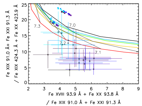
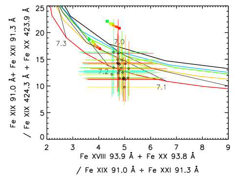
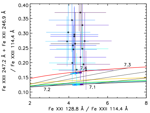
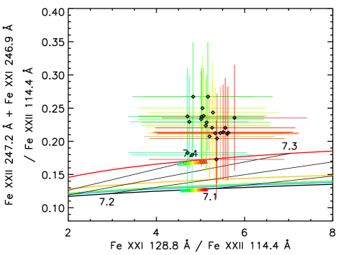
Figure 6: Diagnostics of the electron distribution. Colored curves give the theoretical ratios as a function of $\kappa$. Maxwellian is black, while $\kappa$ = 2 is red. Thin black lines denote isotherms, with the value of log($T$ [K]) indicated. The crosses indicate the observed line intensity ratios and their uncertainties. The color of the crosses denote time during the flare (00:08 – 00:50 UT), as indicated by the color bar. The left panels show results until the peak at 00:25 UT, while the right images show the results during 00:26–00:50 UT. Colored asterisks and triangles denote the theoretical line ratios for Maxwellian and $\kappa$ = 2, folded over the respective DEM${}_{\kappa}(T)$.

4.3.1 Diagnostics from Fe XIX

The sensitivity to $\kappa$ in the first ratio-ratio diagram arises from a combination of the Fe XIX lines at 91.0 Å and 424.3 Å, which are widely separated in wavelength. Both these lines are blended with either Fe XX or Fe XXI. For details, see Appendix A.2. The sensitivity to temperature is obtained from a combination of the 91.0 Å blend with the well-known Fe XVIII line at 93.9 Å, which is also blended with Fe XX (Appendix A.1). The theoretical ratio-ratio diagram is shown in Fig. 6, top. There, the curves shown by full lines denote the theoretical ratios as a function of $\kappa$, with their color-coding is the same as in Figs. 4 and 5. In particular, black lines represent Maxwellian theoretical ratios, and red represents $\kappa$ = 2. Isotherms connecting points with different $\kappa$ but the same log($T$ [K]) are indicated as thin black lines.

The observed ratios and their 1–$\sigma$ uncertainties are shown by diamonds and colored crosses, where the color indicates the time during the flare, starting from 00:08 UT (black and violet) to 00:50 UT (red). Diagnostics prior to 00:80 UT is not possible since the weaker lines cannot be identified in the observed spectra before this time. After 00:80 UT, the results of the diagnostics indicate a range of $\kappa$ values, depending on the time. We note that accurate determination of a $\kappa$ value is not possible due to the large observational uncertainties with respect to the spread of the theoretical curves for different $\kappa$ values. Within the limit of the uncertainties, we can only determine that the plasma is likely extremely non-Maxwellian, with values of $\kappa$ $\lesssim$ 2 diagnosed during the early and impulsive phases of the flare, from 00:08 UT to approximately 00:20 UT (black, violet, and blue; Fig. 6, top left). Subsequently, the plasma thermalizes, with the yellow to red crosses being consistent even with the Maxwellian distribution within their respective uncertainties.

We further note that at around 00:80 UT, some of the observed ratios (black crosses) are far from the diagnostic curves. The cause of this is not clear. It could indicate possible departures of the true electron energy distribution from a $\kappa$-distribution at the start of the flare, or problems with blends or identifications of weaker lines.

Finally, we note that the $T$ diagnosed simultaneously with $\kappa$ is lower than those obtained in Sect. 4.2. In our case, we obtain log($T$ [K]) $\approx$ 7.1–7.2, which is likely caused by the plasma multithermality: The values of $T$ obtained from the ratio-ratio diagrams reflect the $G_{X,ji}(T,n_{\mathrm{e}},\kappa)$ of the ions used to diagnose $T$ and $\kappa$ simultaneously.

4.3.2 Diagnostics from Fe XXII

To verify the results of the non-Maxwellian diagnostics, as well as to perform it from lines formed at higher $T$, we use the Fe XXII ratio-ratio diagrams. The ratio Fe XXII 247.2 Å / 114.4 Å is sensitive to $\kappa$ since it involves lines formed at wavelengths different by about a factor of two. The Fe XXII 247.2 Å line is however blended with Fe XXI (Appendix A.5). The sensitivity to $T$ comes from the combination of Fe XXII 114.4 Å with Fe XXI 128.75 Å.

The theoretical ratio-ratio curves together with the observed intensities are shown in Fig. 6, bottom. Overall, the results confirm the picture obtained from Fe XIX. It is again seen that the plasma is strongly non-Maxwellian during the early and impulsive phases of the flare, while the plasma becomes closer to Maxwellian during the peak and gradual phases. The observed points are however further away from the theoretical ratios than in the case of diagnostics from Fe XIX. This could be at least in part due to the unresolved AR blend of S XI at 246.90 Å (Appendix A.5) that was not included in the theoretical intensity calculations of the Fe XXII+Fe XXI blend at 247.2 Å. This is since sulfur is not a low-FIP element as iron, and thus it could possibly experience anomalous abundances during flares (c.f., Doschek et al., 2015; Doschek & Warren, 2016).

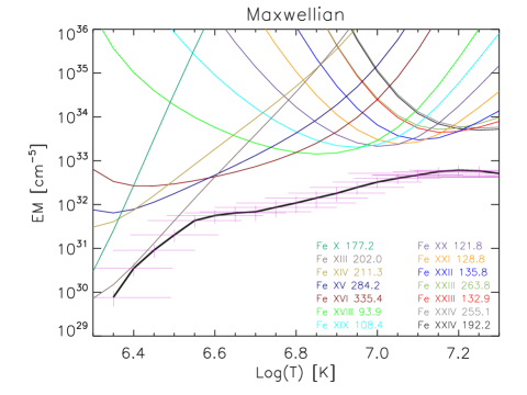
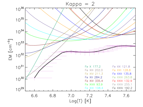
Figure 7: Emission measure distributions and its uncertainties derived from the spectrum at 00:25 UT together with the respective EM-loci plots. The spectral lines used are indicated. Top: EM${}_{\mathrm{Maxw}}(T)$ derived for the Maxwellian distribution. Bottom: The $EM_{\kappa=2}(T)$ derived for $\kappa$ = 2.

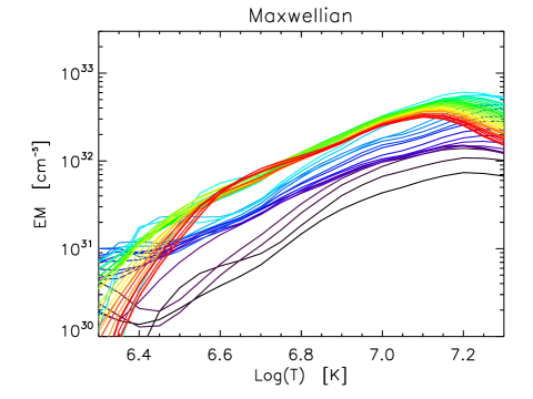
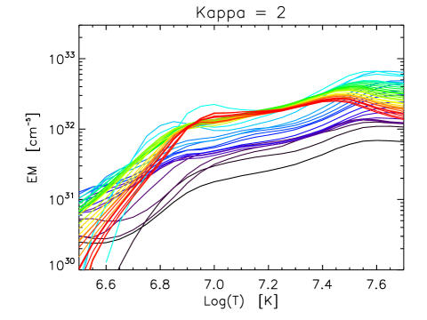
Figure 8: Evolution of the EM(T) distribution during the studied time interval. The colors denotes time during the flare.

4.4 Differential emission measure

In previous Sections 4.2 and 4.3, we obtained different temperatures using line ratios from different ionization stages, suggesting that the plasma is multithermal. This is not surprising, since EVE is a full-Sun spectrometer, and the flare is an eruptive one, i.e., it involves multiple emitting flare loops (Fig. 1c–e).

To quantify the degree of multithermality of the flare, we performed DEM${}_{\kappa}(T)$ analysis using the regularization inversion method of Hannah & Kontar (2012). This method can be straightforwardly generalized for non-Maxwellian distributions simply by supplying it with the non-Maxwellian $G_{X,ji}(T,n_{\mathrm{e}},\kappa)$ (Mackovjak et al., 2014). The advantage of this method is that it provides not only the DEM${}_{\kappa}(T)$, but also its uncertainties in both the DEM and $T$ as well. To reconstruct the DEM, we used the EVE flare lines together with additional well-known lower-$T$ EUV lines to constrain the temperature space. These lower-$T$ lines include the Fe X 177.2 Å, Fe XIII 202.0 Å, Fe XIV 211.3 Å, Fe XV 284.2 Å, and Fe XVI 335.4 Å lines (e.g., O’Dwyer et al., 2010; Warren et al., 2012; Del Zanna, 2013). Especially the Fe X and Fe XIII provide strong constraints (Fig. 7) for temperatures below log($T$ [K]) = 6.3 and 6.6 for Maxwellian and $\kappa$ = 2, respectively. In addition, the line of Fe XIX 108.4 Å was used instead of other Fe XIX lines, since this is the best line for EM analyses, see Del Zanna & Woods (2013).

We first applied this method to obtain the DEM${}_{\kappa}(T)$ for the flare peak at 00:25 UT. The corresponding emission measure distributions EM${}_{\kappa}(T)$, obtained as DEM${}_{\kappa}(T)\mathrm{d}T$, are shown in Fig. 7. There, the EM${}_{\kappa}(T)$ are shown for the Maxwellian and $\kappa$ = 2 together with the respective EM-loci plots (Strong, 1978; Veck et al., 1984; Del Zanna & Mason, 2003; Mackovjak et al., 2014). The EM${}_{\kappa}(T)$ obtained for these two distributions are similar, except a shift towards higher $T$ for $\kappa$ = 2, which occurs mainly as a result of the behavior of the ionization equilibrium with $\kappa$ (see Fig. 3).

Both EM${}_{\kappa}(T)$ distributions are relatively flat at temperatures above log($T$ [K]) = 6.6 and 6.9 for the Maxwellian and $\kappa$ = 2, respectively, indicating strongly multithermal plasma. Their peak occurs at about log($T$ [K]) = 7.2 and 7.5, respectively, and the EM${}_{\kappa}(T)$ decrease only about an order of magnitude between log($T$ [K]) = 6.6–7.2 (Maxwellian) and 6.9–7.6 ($\kappa$ = 2). At lower $T$, the EM${}_{\kappa}(T)$ decrease sharply, mainly as a result of the subtraction of the pre-flare spectrum. It is this decrease that suppresses the QS and AR blends to EVE flare lines (see Appendix A for details).

We note that the high-temperature end of the DEM${}_{\kappa}(T)$ is poorly constrained due to lack of EVE lines formed at temperatures above the formation temperature of Fe XXIV. This ion has maximum of the relative ionization abundance at log($T$ [K]) = 7.25 for Maxwellian and 7.60 for $\kappa$ = 2. This increase with $\kappa$ occurs due to large increase in both ionization and recombination rates with decreasing $\kappa$. Subsequently, the peak of the DEM${}_{\kappa}(T)$ found for this flare occurs close to peak formation temperature of Fe XXIV, i.e., log($T$ [K]) = 7.25 for Maxwellian and 7.60 for $\kappa$ = 2 (Figs. 7 and 8). Such peaks are by necessity poorly constrained as well. However, without observations of the flare plasma in X-rays from either RHESSI or the X-ray Telescope (XRT, Golub et al., 2007) onboard Hinode/XRT, it is not possible to provide accurate high-temperature constraints for our DEMs.

The evolution of the EM${}_{\kappa}(T)$ during the flare is shown in Fig. 8. There, the color-coding of the EM${}_{\kappa}(T)$ curves is the same as in Fig. 6. It is seen that the flat EM${}_{\kappa}(T)$ curves persist throughout the 00:08–00:50 UT period, and that their character do not change strongly over time, except for an increase in the overall emission measure, by about an order of magnitude. Largest EMs occur at about 00:25 UT; i.e., during the peak phase of the soft X-ray flux (c.f., Fig. 1), and persist until the end of the analyzed period 25 min later. Finally, the maxima of the EM${}_{\kappa}(T)$ curves at log($T$ [K]) $\approx$ 7.2 for the Maxwellian and log($T$ [K]) $\approx$ 7.6 for $\kappa$ = 2 occur already at the start of the flare at about 00:08 UT, and persist until about the peak phase at 00:25 UT (blue and cyan color). These maxima are however poorly constrained as discussed above. At later times, the maxima decrease to log($T$ [K]) = 7.1 and 7.4 during the gradual phase (red curves) for the Maxwellian and $\kappa$ = 2, respectively.

4.5 Influence of DEM${}_{\kappa}(T)$ on the diagnostics of $\kappa$

Since the ratio-ratio diagrams used to diagnose $\kappa$ in Sect. 4.3 were constructed under the isothermal assumption, we used the DEM${}_{\kappa}(T)$ obtained in Sect. 4.4 to calculate the DEM-predicted diagnostic line ratios as a function of $\kappa$ (see Eq. 4) and time. This is useful in estimating the theoretical ratios as a function of $\kappa$ for multithermal situations; and it is the same procedure as outlined in Dudík et al. (2015, Sect. 4.3.2 therein).

Effectively, the DEM-predicted line ratios are the ratio-ratio curves weighted by the DEM${}_{\kappa}(T)$. I.e., the DEM-predicted ratios will always lie close to the theoretical curves in the ratio-ratio diagrams; departure from the curve is possible only in the local direction of curvature. This also means that for flat curves, the DEM-predicted ratios will lie very close to the respective curves.

This is indeed what we found. In Fig. 6, the DEM-predicted ratios are shown for the Maxwellian and $\kappa$ = 2 as colored asterisks (for Maxwellian) and triangles (for $\kappa$ = 2), where the color again stands for time. Since the DEM${}_{\kappa}(T)$ do not change their shape appreciably, the DEM-predicted ratios for different times are clustered. The ratio-ratio diagram involving Fe XIX lines contains diagnostic curves that are locally convex; the DEM-predicted ratios then lie above these curves. In particular, the DEM-predicted ratios for $\kappa$ = 2 lie at the ratio-ratio curves corresponding to $\kappa$ = 3–7. However, we note that the distance between the DEM-predicted ratios for the Maxwellian and $\kappa$ = 2 distribution is much smaller than the size of the error-bar of individual observed ratios. This means that only the observed ratios far from the DEM-predicted ratios can be confidently described as strongly non-Maxwellian. These are the ratios detected during the flare start and impulsive phases at about 00:08–00:20 UT (Sect. 4.3.1).

The ratio-ratio diagram involving Fe XXII has much flatter ratio-ratio curves than the one involving Fe XIX, and the DEM-predicted ratios for Maxwellian and $\kappa$ = 2 lie very close to the respective curves as expected. Again, this increases the confidence that the ratios during the start and impulsive phases of the flare are strongly non-Maxwellian.

We however note that some ratios observed at the very start of the flare (black crosses in Fig. 6) are very far from the respective DEM-predicted ones even for $\kappa$ = 2. In the case of Fe XXII, they are away from the DEM-predicted ones by as much as a factor of 2.5. The reason for this is unknown. It is unlikely to be due to the known QS or AR blends (see, e.g., Appendix A). It is possible either that at the start of the flare, the true electron energy distribution is not well-described by a $\kappa$-distribution, or there are other effects at play, such as non-equilibrium ionization, or both. We note that the ionization equilibration timescales in flares can be of the order of seconds, tens of seconds, or possibly even minutes depending on the electron density (Doschek et al., 1979; Doschek & Tanaka, 1987; Golub et al., 1989; Bradshaw et al., 2004; Smith & Hughes, 2010; Polito et al., 2016).The high densities above log$(n_{\mathrm{e}}\,[\mathrm{cm}^{-3}])$ = 11 diagnosed in Sect. 4.1 should strongly suppress the non-equilibrium ionization effects.

5 Summary

We performed the non-Maxwellian diagnostics of the eruptive X5.4-class flare of 2012 March 07 using full-Sun spectra observed by the SDO/EVE instrument. The spectra were averaged over 1 minute during 00:08–00:50 UT and a pre-flare spectrum was subtracted. Theoretical line intensity calculations were performed for the non-Maxwellian $\kappa$-distributions by using the KAPPA database. While these distributions might not totally describe the evolving flare plasma, they allow for modeling of the effect of high-energy tails on the spectra at the expense of only one extra parameter, $\kappa$. The theoretical non-Maxwellian line intensity calculations were compared with the observed ones for a range of ions, from Fe XIX to Fe XXIV. The main findings can be summarized as follows:

1. The electron densities diagnosed using Fe XXI reach log$(n_{\mathrm{e}}\,[\mathrm{cm}^{-3}])$ = 11.5, and do not evolve strongly during the entire studied time interval. The Fe XXI 145.7 / 128.8 Å ratio is not strongly sensitive to either $T$ or $\kappa$, making the electron densities the only plasma parameter independent of the other ones.

2. The temperatures diagnosed under an assumption of a constant $\kappa$ depend strongly on the assumed value of $\kappa$. This is a consequence mainly of the behavior of the ionization equilibrium. The temperatures diagnosed for $\kappa$ = 2 are about a factor of 2 higher than the Maxwellian temperatures. Additionally, the temperatures depend on the line ratios used, with Fe XXII/Fe XX, Fe XXIII/Fe XXI and Fe XXIV/Fe XXII yielding progressively higher temperatures, which is a signature of multithermality.

3. Maxwellian temperatures diagnosed from line ratios are inconsistent with the temperature derived from a ratio of GOES channels. The GOES temperatures are higher than those from the line ratios, as found already by Del Zanna & Woods (2013). We suggest that the $\kappa$-distributions could represent a possible resolution of this discrepancy.

4. The temperatures evolve during the flare, rising at 00:12 UT and peaking at 00:22 UT, after the strongest gradient of the X-ray flux during the impulsive phase, but before the peak of the soft X-ray flux as detected by GOES. The temperatures then decrease afterwards.

5. Extremely non-Maxwellian values of $\kappa$ $\lesssim$ 2 are diagnosed until about 00:20 UT, i.e., during the early and impulsive phases of the flare. Subsequently, the plasma thermalizes, i.e., moves closer to Maxwellian. The error-bars of the observed ratios are however large compared to the spread of the curves for diagnostics of $\kappa$, which precludes determination of $\kappa$ after about 00:20 UT, i.e., during the thermalization.

6. The plasma is found to be multithermal, with relatively flat DEM${}_{\kappa}(T)$ independently of the $\kappa$ value used. The shape of the DEM does not strongly evolve with time, except an overall increase of the total emission measure, and decrease of its peak. The peak occurs at log($T$ [K]) $\approx$ 7.2 and 7.6 for the Maxwellian and $\kappa$ = 2 during the early and impulsive phases of the flare. This peak is however likely poorly constrained due to absence of observations at higher temperatures. The peak subsequently decreased to log($T$ [K]) $\approx$ 7.1 and 7.4 during the gradual phase.

Our results show that the departures from the Maxwellian distribution can be determined using flare lines observed by SDO/EVE. Furthermore, these departures from Maxwellian can be extreme during the early and impulsive phases of the flare. As we have shown, the non-Maxwellian distributions influence both the temperature and DEM diagnostics of the flare plasma. We suggest that these effects ought to be taken into account during such analyses of flare observations, performed by a number of authors in the past (e.g., Hannah & Kontar, 2013; Kennedy et al., 2013; Cheng et al., 2014; Sun et al., 2014; Song et al., 2015; Gou et al., 2015; Scullion et al., 2016; Lee et al., 2017a).

Appendix A EVE lines and their blends

Here, we discuss the details involving individual EVE flare lines used for diagnostics of plasma parameters during the flare, especially $n_{\mathrm{e}}$, $T$, and $\kappa$.

A.1 Fe XVIII

The EVE line at 93.9 Å is a well-known blend of Fe XVIII 93.93 Å with Fe XX 93.78 Å (e.g., O’Dwyer et al., 2010; Lemen et al., 2012; Testa et al., 2012; Warren et al., 2012; Del Zanna & Woods, 2013). Unresolvable blends include Fe VIII, Fe X, Fe XII, Fe XIV, and other QS and AR lines (e.g., O’Dwyer et al., 2010; Del Zanna, 2013; Del Zanna & Woods, 2013) The contribution of these blends is in our case (i.e., for the DEM${}_{\kappa}(T)$ obtained in Sect. 4.4) not significant. Resolvable blends in the wings of the Fe XVIII line include Ni XX 94.50 Å and Fe XX 94.64 Å that were fitted using XCFIT. These blends are typically $<$5% of 93.9 Å line intensity.

A.2 Fe XIX

The EVE line at 91 Å is a blend of Fe XIX 91.01 Å with Fe XXI 91.27 Å. Del Zanna & Woods (2013) lists multiple other unresolvable blends: in quiet Sun (hereafter, QS), Fe X, Fe XI, and Fe XII, while in active region (AR) conditions additional blends occur from Fe XIII, Fe XVI, and O VIII. We re-calculated the total contribution function including all blends, and verified that for the DEM${}_{\kappa}(T)$ derived for the flare (Sect. 4.4) the QS and AR blends at temperatures below log($T$ [K]) = 6.6 are effectively removed by the subtraction of the pre-flare spectrum. The resolvable blends in wings of the 91.0 Å line include Fe XX 90.59 Å and Ni XXIII 91.87 Å, which were approximated using XCFIT. Their intensities are typically $\lesssim$10% of the 91.0 Å line.

The 424.3 Å EVE line is a blend of Fe XIX 424.27 Å with Fe XX 423.93 Å. The unresolvable AR blend of Ar XV 423.98 Å (formed at log($T$ [K]) $\approx$ 6.7 at Maxwellian conditions) was not included in the theoretical intensity calculations. It contributes less than 10%. The resolved blends include Fe XX 423.11 Å, which was included in XCFIT, and Fe XIX 425.21 Å line, which was unobserved and thus not fitted.

Finally, the EVE line of Fe XIX 108.35 Å is the strongest Fe XIX line and thus best for EM analyses (Sect. 4.4), as noted by Del Zanna & Woods (2013). These authors state that this line is blended with Fe XXI, which however contributes only about 10%. This blend has been neglected, since its contribution is smaller than the overall uncertainty of the line, especially considering the 20% EVE calibration uncertainty (Woods et al., 2012).

A.3 Fe XX

The Fe XX 121.85 Å line is a strong line suitable for EM analyses (Del Zanna & Woods, 2013). It has a selfblend at 121.99 Å, whose contribution is $\leq$1% of the main line. The Fe XXI 121.21 Å blend, which broadens the line, was included as an additional Gaussian in XCFIT. Its typical contribution to the total intensity is about 8% of the main line. Several resolved lines nearby include Fe XX 119.98 Å and Fe XXI 123.83 Å, which were fitted by XCFIT. An unknown QS blend at 122.5 Å, possibly Ne VI, was mentioned by Del Zanna & Woods (2013).

A.4 Fe XXI

Both Fe XXI 128.75 Å and 145.73 Å lines used for diagnostics of $n_{\mathrm{e}}$ are well observed by EVE, as already mentioned in Sect. 4.1. The Fe XXI 128.75 Å is relatively free of blends, with only a few QS blends (Del Zanna & Woods, 2013). These QS blends are expected to be negligible in the pre-flare subtracted spectra. We have verified this by including their theoretical contribution as a function of $T$ into the synthetic $G_{X,ji}(T,n_{\mathrm{e}},\kappa)$ and folding over the DEM${}_{\kappa}(T)$ calculated from the observations (see Sect. 4.4). The nearby lines, Fe XX 127.84 Å and Mn XIX 130.58 Å are resolved in EVE spectra and were included in the fitting with XCFIT.

The Fe XXI 145.73 Å is blended by Mn XXI 145.4590 Å. This blend cannot be subtracted during line profile fitting. However, its contribution to the Fe XXI 145.73 Å  intensity is $\leq$10%. The contribution of this blend is not included in our theoretical calculations of the Fe XXI 145.73 Å line. An additional blend could be a Ni X QS line (Del Zanna & Woods, 2013), not included in CHIANTI v7.1 or v8. Its contribution should however be negligible, since it is a QS line. The nearby lines of Ni XXII 144.81 Å and Fe XXIII 147.25 Å are resolved and were included in the fitting with XCFIT together with their blends.

A.5 Fe XXII

The Fe XXII 135.79 Å line (used for diagnostics of $T$ in Sect. 4.2) is a self-blend with the 136.0 Å transition. This line has no other significant blends. Resolved lines nearby include Fe XXII 134.69 Å and Fe XXIII 136.53 Å, which were included in the XCFIT together with their blends.

The Fe XXII line at 114.4 Å used for diagnostics of $\kappa$ (Sect. 4.3) is visible at densities above log$(n_{\mathrm{e}}\,[\mathrm{cm}^{-3}])$ $\approx$ 11.5 (Del Zanna & Woods, 2013). This line does not have any significant unresolved blends. Resolved lines in its vicinity arise from Fe XX at 113.35 Å, Fe XIX at 115.40 Å, and Mn XVIII at 115.37 Å. These lines were included in the Gaussian fitting of the spectra by XCFIT. The QS blends of Fe IX, Fe XI, Ne VI are not significant, and we verified that these are effectively suppressed by the DEM${}_{\kappa}(T)$ obtained in Sect. 4.4.

The Fe XXII line at 247.2 Å used for diagnostics of $\kappa$ is even weaker than the previous one. It is a sum of Fe XXII 247.19 Å with Fe XXI 246.95 Å. These contributions were summed together in theoretical calculations. The unresolved blend from S XI 246.90 Å (formed at about log($T$ [K]) = 6.3 for Maxwellian distribution) was not included. For the DEM${}_{\kappa}(T)$ obtained here, it contributes about 10% to the total observed 247 Å line intensity for coronal abundances of Feldman et al. (1992). Strongest resolved lines in the vicinity include Fe XIII 246.21 Å, Si VI 246.00 Å, and O V 248.46 Å, which can be visible in the subtracted spectrum, and were subsequently fitted by XCFIT.

A.6 Fe XXIII

The Fe XXIII 132.91 Å used for diagnostics of $T$ (Sect. 4.2) is blended with Fe XX 132.84 Å. This blend has been removed using the procedure outlined by Del Zanna & Woods (2013), i.e., from the Fe XX 121.84 Å, since both these Fe XXI lines are decays to the ground state. The additional blend of Fe XIX 132.62 Å is very weak, below 1%.

The Fe XXIII 263.77 Å line used for DEM analysis (Sect. 4.4) has no significant blends.

A.7 Fe XXIV

The Fe XXIV 192.03 Å line used for temperature diagnostics (Sect. 4.2) is a well-known flare line also observed by Hinode/EIS and other instruments (see, e.g., Warren & Reeves, 2001; O’Dwyer et al., 2010, 2011; Hara et al., 2011; Doschek et al., 2013; Young et al., 2013; Graham et al., 2013; Lee et al., 2017b). This line has no significant blends, except the QS O V, Fe XI, and Fe XII (Ko et al., 2009), that are negligible in large flares (Del Zanna & Woods, 2013). Nearby resolved lines of Fe XII 191.05 Å and Ca XVII 192.85 Å were included in the approximation by XCFIT together with their respective blends.

The Fe XXIV 255.11 Å line is blended with Fe XVII 254.89 Å, which contributes about 5% for the DEMs obtained in Sect. 4.4.

A.8 Additional lines used for DEM analyses

Several lines formed at QS or AR temperatures are used for DEM analyses in Sect. 4.4. The Fe X 177.2 Å is blended with Fe IX 176.96 Å, which contributes about 20%. An additional blend of Fe IX 177.6 Å is weaker by a factor of 2–4, depending on $\kappa$ (Dudík et al., 2014b).

The Fe XIII 202.04 Å EVE line is blended with Fe XII 201.74 Å, which contributes about 15 %. The Fe XIV 211.32 Å has no significant blends. The Fe XV 284.16 Å line is blended in EVE spectra with Fe XVII 283.95 Å, which contributes about 5% to the total intensity. Finally, the Fe XVI 335.41 Å is blended with Fe XXI 335.62 Å, which contributes about 5% of the total intensity.

References

- Ajello et al. (2014) Ajello, M., Albert, A., Allafort, A., et al. 2014, ApJ, 789, 20
- Altun et al. (2005) Altun, Z., Yumak, A., Badnell, N. R., Colgan, J., & Pindzola, M. S. 2005, A&A, 433, 395
- Altun et al. (2006) Altun, Z., Yumak, A., Badnell, N. R., Loch, S. D., & Pindzola, M. S. 2006, A&A, 447, 1165
- Altun et al. (2007) Altun, Z., Yumak, A., Yavuz, I., et al. 2007, A&A, 474, 1051
- Aulanier et al. (2012) Aulanier, G., Janvier, M., & Schmieder, B. 2012, A&A, 543, A110
- Badnell (2006) Badnell, N. R. 2006, A&A, 447, 389
- Badnell (2011) —. 2011, Computer Physics Communications, 182, 1528
- Badnell & Griffin (2001) Badnell, N. R., & Griffin, D. C. 2001, Journal of Physics B Atomic Molecular Physics, 34, 681
- Badnell et al. (2001) Badnell, N. R., Griffin, D. C., & Mitnik, D. M. 2001, Journal of Physics B Atomic Molecular Physics, 34, 5071
- Badnell et al. (2003) Badnell, N. R., O’Mullane, M. G., Summers, H. P., et al. 2003, A&A, 406, 1151
- Battaglia & Kontar (2013) Battaglia, M., & Kontar, E. P. 2013, ApJ, 779, 107
- Battaglia et al. (2015) Battaglia, M., Motorina, G., & Kontar, E. P. 2015, ApJ, 815, 73
- Bautista & Badnell (2007) Bautista, M. A., & Badnell, N. R. 2007, A&A, 466, 755
- Berrington & Tully (1997) Berrington, K. A., & Tully, J. A. 1997, A&AS, 126, doi:10.1051/aas:1997384
- Bian et al. (2014) Bian, N. H., Emslie, A. G., Stackhouse, D. J., & Kontar, E. P. 2014, ApJ, 796, 142
- Boerner et al. (2012) Boerner, P., Edwards, C., Lemen, J., et al. 2012, Sol. Phys., 275, 41
- Bradshaw et al. (2004) Bradshaw, S. J., Del Zanna, G., & Mason, H. E. 2004, A&A, 425, 287
- Brown (1971) Brown, J. C. 1971, Sol. Phys., 18, 489
- Brown et al. (2016) Brown, S. A., Fletcher, L., & Labrosse, N. 2016, A&A, 596, A51
- Bykov et al. (2013) Bykov, A. M., Malkov, M. A., Raymond, J. C., Krassilchtchikov, A. M., & Vladimirov, A. E. 2013, Space Sci. Rev., 178, 599
- Cheng et al. (2014) Cheng, X., Ding, M. D., Zhang, J., et al. 2014, ApJ, 789, L35
- Chidichimo et al. (2005) Chidichimo, M. C., Del Zanna, G., Mason, H. E., et al. 2005, A&A, 430, 331
- Chintzoglou et al. (2015) Chintzoglou, G., Patsourakos, S., & Vourlidas, A. 2015, ApJ, 809, 34
- Colgan et al. (2004) Colgan, J., Pindzola, M. S., & Badnell, N. R. 2004, A&A, 417, 1183
- Colgan et al. (2003) Colgan, J., Pindzola, M. S., Whiteford, A. D., & Badnell, N. R. 2003, A&A, 412, 597
- Culhane et al. (2007) Culhane, J. L., Harra, L. K., James, A. M., et al. 2007, Sol. Phys., 243, 19
- De Pontieu et al. (2014) De Pontieu, B., Title, A. M., Lemen, J. R., et al. 2014, Sol. Phys., 289, 2733
- Del Zanna (2006) Del Zanna, G. 2006, A&A, 459, 307
- Del Zanna (2013) —. 2013, A&A, 558, A73
- Del Zanna et al. (2005) Del Zanna, G., Chidichimo, M. C., & Mason, H. E. 2005, A&A, 432, 1137
- Del Zanna et al. (2015) Del Zanna, G., Dere, K. P., Young, P. R., Landi, E., & Mason, H. E. 2015, A&A, 582, A56
- Del Zanna & Mason (2003) Del Zanna, G., & Mason, H. E. 2003, A&A, 406, 1089
- Del Zanna & Woods (2013) Del Zanna, G., & Woods, T. N. 2013, A&A, 555, A59
- Dere (2007) Dere, K. P. 2007, A&A, 466, 771
- Dere et al. (1997) Dere, K. P., Landi, E., Mason, H. E., Monsignori Fossi, B. C., & Young, P. R. 1997, A&AS, 125, 149
- Dere et al. (2009) Dere, K. P., Landi, E., Young, P. R., et al. 2009, A&A, 498, 915
- Doschek et al. (1979) Doschek, G. A., Kreplin, R. W., & Feldman, U. 1979, ApJ, 233, L157
- Doschek & Tanaka (1987) Doschek, G. A., & Tanaka, K. 1987, ApJ, 323, 799
- Doschek & Warren (2016) Doschek, G. A., & Warren, H. P. 2016, ApJ, 825, 36
- Doschek et al. (2015) Doschek, G. A., Warren, H. P., & Feldman, U. 2015, ApJ, 808, L7
- Doschek et al. (2013) Doschek, G. A., Warren, H. P., & Young, P. R. 2013, ApJ, 767, 55
- Dudík et al. (2014a) Dudík, J., Del Zanna, G., Dzifčáková, E., Mason, H. E., & Golub, L. 2014a, ApJ, 780, L12
- Dudík et al. (2014b) Dudík, J., Del Zanna, G., Mason, H. E., & Dzifčáková, E. 2014b, A&A, 570, A124
- Dudík et al. (2012) Dudík, J., Kašparová, J., Dzifčáková, E., Karlický, M., & Mackovjak, Š. 2012, A&A, 539, A107
- Dudík et al. (2017a) Dudík, J., Polito, V., Dzifčáková, E., Del Zanna, G., & Testa, P. 2017a, ApJ, 842, 19
- Dudík et al. (2017b) Dudík, J., Zuccarello, F. P., Aulanier, G., Schmieder, B., & Démoulin, P. 2017b, ApJ, 844, 54
- Dudík et al. (2015) Dudík, J., Mackovjak, Š., Dzifčáková, E., et al. 2015, ApJ, 807, 123
- Dudík et al. (2017c) Dudík, J., Dzifčáková, E., Meyer-Vernet, N., et al. 2017c, Sol. Phys., 292, 100
- Dungey (153) Dungey, J. W. 153, Phil. Mag., 44
- Dzifčáková (2002) Dzifčáková, E. 2002, Sol. Phys., 208, 91
- Dzifčáková (2006) —. 2006, Sol. Phys., 234, 243
- Dzifčáková & Dudík (2013) Dzifčáková, E., & Dudík, J. 2013, ApJS, 206, 6
- Dzifčáková et al. (2015) Dzifčáková, E., Dudík, J., Kotrč, P., Fárník, F., & Zemanová, A. 2015, ApJS, 217, 14
- Dzifčáková & Kulinová (2010) Dzifčáková, E., & Kulinová, A. 2010, Sol. Phys., 263, 25
- Dzifčáková (1992) Dzifčáková, E. 1992, Sol. Phys., 140, 247
- Emslie et al. (2012) Emslie, A. G., Dennis, B. R., Shih, A. Y., et al. 2012, ApJ, 759, 71
- Feldman et al. (1992) Feldman, U., Mandelbaum, P., Seely, J. F., Doschek, G. A., & Gursky, H. 1992, ApJS, 81, 387
- Fletcher et al. (2011) Fletcher, L., Dennis, B. R., Hudson, H. S., et al. 2011, Space Sci. Rev., 159, 19
- Glesener et al. (2017) Glesener, L., Krucker, S., Hannah, I. G., et al. 2017, ApJ, 845, 122
- Golub et al. (1989) Golub, L., Hartquist, T. W., & Quillen, A. C. 1989, Sol. Phys., 122, 245
- Golub et al. (2007) Golub, L., Deluca, E., Austin, G., et al. 2007, Sol. Phys., 243, 63
- Gou et al. (2015) Gou, T., Liu, R., & Wang, Y. 2015, Sol. Phys., 290, 2211
- Graham et al. (2013) Graham, D. R., Hannah, I. G., Fletcher, L., & Milligan, R. O. 2013, ApJ, 767, 83
- Gu (2003) Gu, M. F. 2003, ApJ, 582, 1241
- Hahn & Savin (2015) Hahn, M., & Savin, D. W. 2015, ApJ, 809, 178
- Hannah et al. (2008) Hannah, I. G., Christe, S., Krucker, S., et al. 2008, ApJ, 677, 704
- Hannah & Kontar (2012) Hannah, I. G., & Kontar, E. P. 2012, A&A, 539, A146
- Hannah & Kontar (2013) —. 2013, A&A, 553, A10
- Hara et al. (2011) Hara, H., Watanabe, T., Harra, L. K., Culhane, J. L., & Young, P. R. 2011, ApJ, 741, 107
- Harra et al. (2016) Harra, L. K., Schrijver, C. J., Janvier, M., et al. 2016, Sol. Phys., 291, 1761
- Hasegawa et al. (1985) Hasegawa, A., Mima, K., & Duong-van, M. 1985, Physical Review Letters, 54, 2608
- Holman et al. (2003) Holman, G. D., Sui, L., Schwartz, R. A., & Emslie, A. G. 2003, ApJ, 595, L97
- Holman et al. (2011) Holman, G. D., Aschwanden, M. J., Aurass, H., et al. 2011, Space Sci. Rev., 260
- Janvier (2017) Janvier, M. 2017, Journal of Plasma Physics, 83, 535830101
- Janvier et al. (2015) Janvier, M., Aulanier, G., & Démoulin, P. 2015, Sol. Phys., 290, 3425
- Janvier et al. (2013) Janvier, M., Aulanier, G., Pariat, E., & Démoulin, P. 2013, A&A, 555, A77
- Jeffrey et al. (2016) Jeffrey, N. L. S., Fletcher, L., & Labrosse, N. 2016, A&A, 590, A99
- Jeffrey et al. (2017) —. 2017, ApJ, 836, 35
- Kašparová & Karlický (2009) Kašparová, J., & Karlický, M. 2009, A&A, 497, L13
- Kennedy et al. (2013) Kennedy, M. B., Milligan, R. O., Mathioudakis, M., & Keenan, F. P. 2013, ApJ, 779, 84
- Ko et al. (2009) Ko, Y.-K., Doschek, G. A., Warren, H. P., & Young, P. R. 2009, ApJ, 697, 1956
- Kontar et al. (2011) Kontar, E. P., Brown, J. C., Emslie, A. G., et al. 2011, Space Sci. Rev., 279
- Kouloumvakos et al. (2016) Kouloumvakos, A., Patsourakos, S., Nindos, A., et al. 2016, ApJ, 821, 31
- Krucker et al. (2008) Krucker, S., Battaglia, M., Cargill, P. J., et al. 2008, A&A Rev., 16, 155
- Kuhar et al. (2016) Kuhar, M., Krucker, S., Martínez Oliveros, J. C., et al. 2016, ApJ, 816, 6
- Laming & Lepri (2007) Laming, J. M., & Lepri, S. T. 2007, ApJ, 660, 1642
- Landi & Gu (2006) Landi, E., & Gu, M. F. 2006, ApJ, 640, 1171
- Landi et al. (2013) Landi, E., Young, P. R., Dere, K. P., Del Zanna, G., & Mason, H. E. 2013, ApJ, 763, 86
- Lee et al. (2017a) Lee, J.-Y., Raymond, J. C., Reeves, K. K., Moon, Y.-J., & Kim, K.-S. 2017a, ApJ, 844, 3
- Lee et al. (2017b) Lee, K.-S., Imada, S., Watanabe, K., Bamba, Y., & Brooks, D. H. 2017b, ApJ, 836, 150
- Lemen et al. (2012) Lemen, J. R., Title, A. M., Akin, D. J., et al. 2012, Sol. Phys., 275, 17
- Lin & Hudson (1971) Lin, R. P., & Hudson, H. S. 1971, Sol. Phys., 17, 412
- Lin et al. (2002) Lin, R. P., Dennis, B. R., Hurford, G. J., et al. 2002, Sol. Phys., 210, 3
- Livadiotis (2015) Livadiotis, G. 2015, Journal of Geophysical Research (Space Physics), 120, 1607
- Mackovjak et al. (2014) Mackovjak, Š., Dzifčáková, E., & Dudík, J. 2014, A&A, 564, A130
- Mason et al. (1984) Mason, H. E., Bhatia, A. K., Neupert, W. M., Swartz, M., & Kastner, S. O. 1984, Sol. Phys., 92, 199
- Mason et al. (1979) Mason, H. E., Doschek, G. A., Feldman, U., & Bhatia, A. K. 1979, A&A, 73, 74
- Mason & Monsignori Fossi (1994) Mason, H. E., & Monsignori Fossi, B. C. 1994, A&A Rev., 6, 123
- Meyer-Vernet (2007) Meyer-Vernet, N. 2007, Basics of the Solar Wind (Cambridge University Press)
- Milligan et al. (2012) Milligan, R. O., Kennedy, M. B., Mathioudakis, M., & Keenan, F. P. 2012, ApJ, 755, L16
- Mitnik & Badnell (2004) Mitnik, D. M., & Badnell, N. R. 2004, A&A, 425, 1153
- Nikolić et al. (2010) Nikolić, D., Gorczyca, T. W., Korista, K. T., & Badnell, N. R. 2010, A&A, 516, A97
- O’Dwyer et al. (2011) O’Dwyer, B., Del Zanna, G., Mason, H. E., et al. 2011, A&A, 525, A137
- O’Dwyer et al. (2010) O’Dwyer, B., Del Zanna, G., Mason, H. E., Weber, M. A., & Tripathi, D. 2010, A&A, 521, A21
- Oka et al. (2013) Oka, M., Ishikawa, S., Saint-Hilaire, P., Krucker, S., & Lin, R. P. 2013, ApJ, 764, 6
- Oka et al. (2015) Oka, M., Krucker, S., Hudson, H. S., & Saint-Hilaire, P. 2015, ApJ, 799, 129
- Olbert (1968) Olbert, S. 1968, in Astrophysics and Space Science Library, Vol. 10, Physics of the Magnetosphere, ed. R. D. L. Carovillano & J. F. McClay, 641
- Owocki & Scudder (1983) Owocki, S. P., & Scudder, J. D. 1983, ApJ, 270, 758
- Parker (1957) Parker, E. N. 1957, J. Geophys. Res., 62, 509
- Patsourakos et al. (2016) Patsourakos, S., Georgoulis, M. K., Vourlidas, A., et al. 2016, ApJ, 817, 14
- Pesnell et al. (2012) Pesnell, W. D., Thompson, B. J., & Chamberlin, P. C. 2012, Sol. Phys., 275, 3
- Petkaki et al. (2012) Petkaki, P., Del Zanna, G., Mason, H. E., & Bradshaw, S. J. 2012, A&A, 547, A25
- Phillips et al. (2008) Phillips, K. J. H., Feldman, U., & Landi, E. 2008, Ultraviolet and X-ray Spectroscopy of the Solar Atmosphere (Cambridge University Press)
- Pierrard & Lazar (2010) Pierrard, V., & Lazar, M. 2010, Sol. Phys., 267, 153
- Polito et al. (2017) Polito, V., Del Zanna, G., Valori, G., et al. 2017, A&A, 601, A39
- Polito et al. (2016) Polito, V., Reep, J. W., Reeves, K. K., et al. 2016, ApJ, 816, 89
- Priest & Forbes (2000) Priest, E., & Forbes, T. 2000, Magnetic Reconnection
- Saint-Hilaire et al. (2008) Saint-Hilaire, P., Krucker, S., & Lin, R. P. 2008, Sol. Phys., 250, 53
- Schrijver & Higgins (2015) Schrijver, C. J., & Higgins, P. A. 2015, Sol. Phys., 290, 2943
- Scudder & Karimabadi (2013) Scudder, J. D., & Karimabadi, H. 2013, ApJ, 770, 26
- Scudder & Olbert (1979) Scudder, J. D., & Olbert, S. 1979, J. Geophys. Res., 84, 2755
- Scullion et al. (2016) Scullion, E., Rouppe van der Voort, L., Antolin, P., et al. 2016, ApJ, 833, 184
- Simões et al. (2013) Simões, P. J. A., Fletcher, L., Hudson, H. S., & Russell, A. J. B. 2013, ApJ, 777, 152
- Simões et al. (2015) Simões, P. J. A., Graham, D. R., & Fletcher, L. 2015, Sol. Phys., 290, 3573
- Smith & Hughes (2010) Smith, R. K., & Hughes, J. P. 2010, ApJ, 718, 583
- Song et al. (2015) Song, H. Q., Chen, Y., Zhang, J., et al. 2015, ApJ, 808, L15
- Strong (1978) Strong, K. T. 1978, PhD thesis, , Univ. College London, (1978)
- Sun et al. (2014) Sun, J. Q., Cheng, X., & Ding, M. D. 2014, ApJ, 786, 73
- Sun et al. (2013) Sun, X., Hoeksema, J. T., Liu, Y., et al. 2013, ApJ, 778, 139
- Sweet (1958) Sweet, P. A. 1958, in IAU Symposium, Vol. 6, Electromagnetic Phenomena in Cosmical Physics, ed. B. Lehnert, 123
- Syntelis et al. (2016) Syntelis, P., Gontikakis, C., Patsourakos, S., & Tsinganos, K. 2016, A&A, 588, A16
- Tandberg-Hanssen & Emslie (1988) Tandberg-Hanssen, E., & Emslie, A. G. 1988, The physics of solar flares
- Testa et al. (2012) Testa, P., Drake, J. J., & Landi, E. 2012, ApJ, 745, 111
- Vasyliunas (1968a) Vasyliunas, V. M. 1968a, J. Geophys. Res., 73, 2839
- Vasyliunas (1968b) Vasyliunas, V. M. 1968b, in Astrophysics and Space Science Library, Vol. 10, Physics of the Magnetosphere, ed. R. D. L. Carovillano & J. F. McClay, 622
- Veck et al. (1984) Veck, N. J., Strong, K. T., Jordan, C., et al. 1984, MNRAS, 210, 443
- Veronig et al. (2010) Veronig, A. M., Rybák, J., Gömöry, P., et al. 2010, ApJ, 719, 655
- Warren & Reeves (2001) Warren, H. P., & Reeves, K. K. 2001, ApJ, 554, L103
- Warren et al. (2012) Warren, H. P., Winebarger, A. R., & Brooks, D. H. 2012, ApJ, 759, 141
- Whiteford et al. (2002) Whiteford, A. D., Badnell, N. R., Ballance, C. P., et al. 2002, Journal of Physics B Atomic Molecular Physics, 35, 3729
- Whiteford et al. (2001) —. 2001, Journal of Physics B Atomic Molecular Physics, 34, 3179
- Witthoeft et al. (2006) Witthoeft, M. C., Badnell, N. R., del Zanna, G., Berrington, K. A., & Pelan, J. C. 2006, A&A, 446, 361
- Witthoeft et al. (2007) Witthoeft, M. C., Del Zanna, G., & Badnell, N. R. 2007, A&A, 466, 763
- Woods et al. (2012) Woods, T. N., Eparvier, F. G., Hock, R., et al. 2012, Sol. Phys., 275, 115
- Wright et al. (2017) Wright, P. J., Hannah, I. G., Grefenstette, B. W., et al. 2017, ApJ, 844, 132
- Young et al. (2013) Young, P. R., Doschek, G. A., Warren, H. P., & Hara, H. 2013, ApJ, 766, 127
- Zatsarinny et al. (2006) Zatsarinny, O., Gorczyca, T. W., Fu, J., et al. 2006, A&A, 447, 379
- Zatsarinny et al. (2005a) Zatsarinny, O., Gorczyca, T. W., Korista, K. T., et al. 2005a, A&A, 438, 743
- Zatsarinny et al. (2005b) —. 2005b, A&A, 440, 1203
- Zharkova et al. (2011) Zharkova, V. V., Arzner, K., Benz, A. O., et al. 2011, Space Sci. Rev., 156
- Zweibel & Yamada (2009) Zweibel, E. G., & Yamada, M. 2009, ARA&A, 47, 291