An Improved Analysis of Least Squares Superposition Codes with Bernoulli Dictionary

Abstract

For the additive white Gaussian noise channel with average power constraint, sparse superposition codes, proposed by Barron and Joseph in 2010, achieve the capacity. While the codewords of the original sparse superposition codes are made with a dictionary matrix drawn from a Gaussian distribution, we consider the case that it is drawn from a Bernoulli distribution. We show an improved upper bound on its block error probability with least squares decoding, which is fairly simplified and tighter bound than our previous result in 2014.

I Introduction

We argue the error probability of superposition codes [6, 7] with Bernoulli dictionary and least squares decoding. In this paper, we improve the upper bound of the error probability shown in [12]. The obtained bound is tighter and is in a simpler form than the previous result.

Sparse superposition codes proposed by Barron and Joseph are applied on the Additive White Gaussian Noise (AWGN) channel and shown to achieve the capacity [6, 7]. In the coding of sparse superposition codes, we generate a real valued matrix, which we call dictionary, then make codewords by superposition of column vectors from the dictionary. Namely, codewords vector $c$ is described with the matrix $X$ and a coefficient vector $\beta$ as follows;

$$c=X\beta.$$

In the original sparse superposition codes, we make a dictionary by drawing from a Gaussian distribution. Using this Gaussian dictionary, the error probability with least square decoding is shown to be

$$O\left(\exp\left\{-(d(C-R)^{2}-\log n/n)n\right\}\right),$$ (1)

where $d$ is a certain positive constant, $n$ is code length, $R$ is a transmission rate, and $C$ is a channel capacity [6]. The bound (1) is exponentially small in $n$ when $R$ satisfies

$$|C-R|=\Omega((\log n)^{1/2}/n^{1/2}).$$ (2)

However, it is difficult to realize the Gaussian dictionary in a real device since the Gaussian random variable can take arbitrary large or small value. In [12], we studied the case that the dictionary is drawn from the unbiased Bernoulli distribution. Namely, each entry of the dictionary only takes $+1$ or $-1$ with probability $1/2$, respectively. We proved that the error probability with Bernoulli dictionary with least square decoding is

$$O\left(\exp\left\{-(d(C-R)^{2}-\log n/n^{1/4})n\right\}\right).$$ (3)

Although the above bound is worse than (1), it is exponentially small in $n$ when $R$ satisfies

$$|C-R|=\Omega((\log n)^{1/2}/n^{1/8}).$$ (4)

To show the above bound, we analyzed the error between binomial and Gaussian distributions, where evaluation of sectional measurement is one of important factors [12]. However, we found the sectional measurement in the analysis loose. Concretely we found that it is better to use Euler-Maclaurin formula in that analysis. Then the above bound (3) is refined as

$$O\left(\exp\left\{-(d(C-R)^{2}-1/n^{1/2})n\right\}\right).$$ (5)

Comparing the above bound to (3), $\log n/n^{1/4}$ is reduced to $1/n^{1/2}$. Consequently, the condition (4) is improved to

$$|C-R|=\Omega(1/n^{1/4}).$$ (6)

In this paper, we treat the least squares decoder, which is optimal in terms of error probability, but computationally intractable. Efficient decoding algorithms are also researched until now, such as [1, 2, 3, 5, 7, 8, 9]. For the efficient decoding algorithms [7], the block error probability is

$$O\left(\exp\left\{-d(C_{n}-R)^{2}n\right\}\right),$$ (7)

where $R<C_{n}<C$ and

$$(C-C_{n})/C=O(\log\log n/\log n).$$ (8)

The above bound is exponentially small while there is a considerable gap between $C_{n}$ and $C$ for the practical code length. It is still an open problem to show that sparse superposition codes with Bernoulli dictionary achieve the capacity with efficient algorithms.

We review the sparse superposition codes in Section II. In section III, we show the new upper bound of the error probability with Bernoulli dictionary. Section IV provides proofs of some lemmas used in Section III.

II Sparse superposition codes

In this section, we review the sparse superposition codes and show the performance of Gaussian dictionary with the least squares estimator.

In the following, ‘$\log$’ denotes the logarithm of base 2 and ‘$\ln$’ denotes the natural logarithm. Gaussian distribution with mean $\mu$ and variance $\sigma^{2}$ is denoted by $N(\mu,\sigma^{2})$.

II-A Problem setting

We consider communication via the AWGN channel. Assume that a message is a $K$ bit string $u\in\{0,1\}^{K}$ and that it is generated from the uniform distribution on $\{0,1\}^{K}$. We use a real value vector $c\in\Re^{n}$ as a codeword to send a message. The codeword $c$ is polluted by the Gaussian noise in the channel. Namely, letting $Y\in\Re^{n}$ be the output of the channel, we have

$$Y=c+\epsilon,$$

where $\epsilon$ is a real number string with length $n$ and each coordinate is independently subject to $N(0,\sigma^{2})$. The power of $c$ is defined as $(1/n)\sum_{i=1}^{n}c_{i}^{2}$ and it is constrained to be not more than $P$ averagely. We also define a signal-to-noise ratio as $v=P/\sigma^{2}$.

We consider the task to estimate the message $u$ based on $Y$ and $X$. Let $\hat{u}$ be an estimated $u$. We call the event $\hat{u}\neq u$ “block error”. Further, we define the transmission rate $R$ as $K/n$. It is desired that we transmit messages at large $R$ with sufficiently small block error probability. It is well known that at all rate less than

$$C=\frac{1}{2}\log(1+v)\ {\rm(bit/transmission)},$$

we can transmit messages with arbitrary small block error probability for sufficiently large $n$.

II-B Coding

We state the coding method of sparse superposition codes. First, we map a message $u$ into a coefficient vector $\beta\in\{0,1\}^{N}$ by a one to one function. The vector $\beta$ is split into $L$ sections of size $M$ and each section has one nonzero element and the other elements are all zero. Then the codeword $c$ is formed as follows:

$$c=X\beta=\beta_{1}X_{1}+\beta_{2}X_{2}+\cdots+\beta_{N}X_{N},$$

where $X$ is an $n\times N$ matrix (dictionary) and $X_{j}$ is the $j$th column vector of $X$. Thus $c$ is a superposition of $L$ column vectors of $X$, with exactly one column selected from each section. We illustrate an example of coding method in Fig.1.

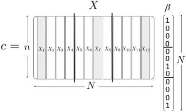
Figure 1: Coding method with $L=3$, $M=4$, $N=12$

In this paper, we set all nonzero elements 1. On the other hand, for the efficient decoding algorithms such as the addaptive successive decoder proposed in [7], we set nonzero elements decaying exponentially among sections. However, we do not treat it here.

In the original paper [6], each element of the dictionary $X$ is independently drawn from $N(0,P/L)$. This distribution is optimal for the random coding argument used to prove the channel coding theorem for the AWGN channel with average power constraint by $P$ [11]. While in this paper, we analyze the case in which each entry of the dictionary is independently drawn as the following random variable:

$$X_{ij}=\left\{\begin{array}[]{l}-\sqrt{P/L}\ ({\rm with\ probability}\ 1/2)\\ \sqrt{P/L}\ ({\rm otherwise})\end{array}\right.$$

The parameters $L$, $M$, and $N$ are selected so as to satisfy the following. The number of messages is $2^{K}$ according to our problem setting about $u$, and the number of codewords is $M^{L}$ according to the way of making $\beta$. Thus we arrange $2^{K}=M^{L}$, equivalently, $K=L\log M$. According to the original paper [6], the value of $M$ is set to be $L^{a}$ and the parameter $a$ is referred to as section size rate. Then we have $K=aL\log L$ and $n=(aL\log L)/R$.

II-C Decoding

We analyze the least squares estimator, which makes the error probability minimum ignoring computational complexity. From the received word $Y$ and knowledge of the dictionary $X$, we estimates the original message $u$, equivalently, estimates the corresponding $\beta$.

Define a set ${\cal B}$ as

$${\cal B}=\{\beta\in\{0,1\}^{N}|\beta_{j}\ {\rm has\ one\ }1\ {\rm in\ each\ section}\}.$$

Then the least squares decoder $\hat{\beta}$ is denoted as

$$\hat{\beta}=\arg\min_{\beta\in{\cal B}}\|Y-X\beta\|^{2},$$

where $\|\cdot\|$ denotes the Euclidean norm.

Let $\beta^{*}$ denote the true $\beta$, then the event $\hat{\beta}\neq\beta^{*}$ corresponds to the block error. Let $mistakes$ denote the number of sections in which the position of the nonzero element in $\hat{\beta}$ is different from that in the $\beta^{*}$. Define the error event ${\cal E}_{\alpha_{0}}=\{mistakes\geq\alpha_{0}L\},$ that the decoder makes $mistakes$ in at least $\alpha_{0}$ fraction of sections. A proportion of $mistakes$ $\alpha=mistakes/L$ is called section error rate.

II-D Performance

It is proved in the paper [6] that given $0<\alpha_{0}\leq 1$, the probability of the event ${\cal E}_{\alpha_{0}}$ is exponentially small in $n$. The following theorem (Proposition 1 in [6]) provides an upper bound on the probability of the event ${\cal E}_{\alpha_{0}}$, where

$$w_{v}=\frac{v}{[4(1+v)^{2}]\sqrt{1+(1/4)v^{3}/(1+v)}}$$

and $g(x)=\sqrt{1+4x^{2}}-1$. It follows that

$$g(x)\geq\min\{\sqrt{2}x,x^{2}\}\ \ {\rm for\ all}\ \ x\geq 0.$$

The definition of $a_{v,L}$ in the statement is given later as (13).

Theorem 1 (Joseph and Barron 2012)

Suppose that each entry of $X$ is independently drawn from $N(0,P/L)$. Assume $M=L^{a}$, where $a\geq a_{v,L}$, and the rate $R$ is less than the capacity $C$. Then

$$\Pr[{\cal E}_{\alpha_{0}}]=e^{-nE(\alpha_{0},R)}$$

with $E(\alpha_{0},R)\geq h(\alpha_{0},C-R)-(\ln(2L))/n$, where

$$h(\alpha,\Delta)=\min\left\{\alpha w_{v}\Delta,\frac{1}{4}g\left(\frac{\Delta}{2\sqrt{v}}\right)\right\}$$

is evaluated at $\alpha=\alpha_{0}$ and $\Delta=C-R$.

Remark: In this theorem, the unit of $R$ and $C$ is nat/transmission. Then, since $n=(aL\ln L)/R$, $L$ is bounded by $nR/a$ when $\ln L\geq 1$.

As noted in Joseph and Barron [6], in order to bound the block error probability, we can use composition with an outer Reed-Solomon (RS) code [10] of rate near one. If $R_{outer}=1-\delta$ is the rate of an RS code, with $0<\delta<1$, then section error rates less than $\delta/2$ can be corrected. Thus, through concatenation with an outer RS code, we get a code with rate $(1-2\alpha_{0})R$ and block error probability less than or equal to $\Pr[{\cal E}_{\alpha_{0}}]$. Arrange as $R=C-\Delta$ and $\alpha_{0}=\Delta$, with $\Delta>0$. Then the overall rate $(1-2\Delta)(C-\Delta)$ continues to have drop from capacity of order $\Delta$. The composite code have block error probability of order $\exp\{-nd\Delta^{2}\}$, where $d$ is a positive constant.

To prove Theorem 1, we evaluate the probability of the event $E_{l}=\{mistakes=l\}$ for $l=1,2,\ldots,L$. The probability $\Pr[E_{l}]$ is used to evaluate

$$\Pr[{\cal E}_{\alpha_{0}}]=\sum_{l\geq\alpha_{0}L}\Pr[E_{l}].$$

We introduce the function $C_{\alpha}=(1/2)\ln(1+\alpha v)$ for $0\leq\alpha\leq 1$. It equals the channel capacity $C$ when $\alpha=1$. Then $C_{\alpha}-\alpha C$ is a nonnegative function which equals $0$ when $\alpha$ is $0$ or $1$ and is strictly positive in between. Thus the quantity $C_{\alpha}-\alpha R$ is larger than $\alpha(C-R)$, which is positive when $R<C$.

For a positive $\Delta$ and $\rho\in[-1,1]$, we define a quantity $D(\Delta,1-\rho^{2})$ as

$$D(\Delta,1-\rho^{2})=\max_{\lambda\geq 0}\Bigl{\{}\lambda\Delta+\frac{1}{2}\ln(1-\lambda^{2}(1-\rho^{2}))\Bigr{\}}$$ (10)

and $D_{1}(\Delta,1-\rho^{2})$ as

$$D_{1}(\Delta,1-\rho^{2})=\max_{0\leq\lambda\leq 1}\Bigl{\{}\lambda\Delta+\frac{1}{2}\ln(1-\lambda^{2}(1-\rho^{2}))\Bigr{\}}.$$ (11)

Note that these quantities are nonnegative.

The following lemma (Lemma 4 in [6]) provides an upper bound on $\Pr[E_{l}]$.

Lemma 2 (Joseph and Barron 2012)

Suppose that each entry of $X$ is independently drawn from $N(0,P/L)$. Let a positive integer $l\leq L$ be given and let $\alpha=l/L$. Then, $\Pr[E_{l}]$ is bounded by the minimum for $t_{\alpha}$ in the interval $[0,C_{\alpha}-\alpha R]$ of $err_{Gauss}(\alpha)$, where

$$err_{Gauss}(\alpha) = {{}_{L}C_{\alpha L}}\exp\{-nD_{1}(\Delta_{\alpha},1-\rho_{1}^{2})\}$$ (12)

$$+\exp\{-nD(t_{\alpha},1-\rho_{2}^{2})\}$$

with $\Delta_{\alpha}=C_{\alpha}-\alpha R-t_{\alpha}$, $1-\rho_{1}^{2}=\alpha(1-\alpha)v/(1+\alpha v)$, and $1-\rho_{2}^{2}=\alpha^{2}v/(1+\alpha^{2}v)$.

To make (12) exponentially small, it is sufficient that the section size rate $a$ is larger than

$$a_{v,L}=\max_{\alpha\in\{\frac{1}{L},\frac{2}{L},\ldots,1-\frac{1}{L}\}}\frac{R\ln{}_{L}C_{L\alpha}}{D_{1}(C_{\alpha}-\alpha C,1-\rho_{1}^{2})L\ln L}.$$ (13)

The quantity $a_{v,L}$ converges to a finite value as $L$ goes to infinity (see Lemma 5 in [6]).

III Main results

In this section, we analyze the performance of sparse superposition codes with Bernoulli dictionary. The result stated here is an improvement of the result in [12], where we use the same code. We improve the upper bound of the error probability by refining some lemmas used in [12]. First, we state the main theorem in this paper.

Theorem 3

Suppose that each entry of $X$ is independent equiprobable $\pm\sqrt{P/L}$. Assume $M=L^{a}$, where $a\geq a_{v,L}$, and rate $R$ is less than capacity $C$. Then,

$$\Pr[{\cal E}_{\alpha_{0}}]=e^{-nE(\alpha_{0},R)}$$

with

$$E(\alpha_{0},R)\geq h(\alpha_{0},C-R)-(\ln(2L))/n-\iota(L),$$

where $\iota(L)=\max\{\iota_{1},\iota_{2}\}$, which are defined in Lemma 4.

Remark: This theorem is the correspondent of Theorem 1 in Bernoulli dictionary case and the error exponent is worse than that in Theorem 1 by $\iota(L)$. This theorem is the same form as the previous result in Theorem 5 in [12], however $\iota(L)$ converges to zero more rapidly than that in the previous result as details mentioned later.

In order to prove Theorem 3, we use the following lemma, which is the correspondent in this case to Lemma 2. The definition of $\iota_{1}$ and $\iota_{2}$ in Theorem 3 is given in the following lemma.

Lemma 4

Suppose that each entry of $X$ is independently equiprobable $\pm\sqrt{P/L}$. Let $\alpha_{0}$ be a certain real number in $(0,1]$ and $\alpha=l/L$. Then, for every $L\geq 2$ and for all $l$ such that $\alpha_{0}\leq\alpha\leq 1$, $\Pr[E_{l}]$ is bounded by the minimum for $t_{\alpha}$ in the interval $[0,C_{\alpha}-\alpha R]$ of $err_{Ber}(\alpha)$, where

$$err_{Ber}(\alpha) = {{}_{L}C_{\alpha L}}\exp\{-n(D_{1}(\Delta_{\alpha},1-\rho_{1}^{2})-\iota_{1})\}$$

$$+\exp\{-n(D(t_{\alpha},1-\rho_{2}^{2})-\iota_{2})\}$$

with $\Delta_{\alpha}=C_{\alpha}-\alpha R-t_{\alpha}$, $1-\rho_{1}^{2}=\alpha(1-\alpha)v/(1+\alpha v)$, and $1-\rho_{2}^{2}=\alpha^{2}v/(1+\alpha^{2}v)$. The variables $\iota_{1}$ and $\iota_{2}$ are defined by the following series of equations

$$\iota_{1} = \ln((1+\iota_{3})(1+\max\{\iota_{4},\iota_{5}\}))$$

$$\iota_{2} = \phi(L)+\ln\left(1+\frac{2\eta}{L}\right)$$

where

$$1+\iota_{3} = \max_{\alpha_{0}L\leq l\leq L}\left(e^{\phi(l)}\left(1+\frac{\eta(1+v)}{l}\right)\right)$$

$$1+\iota_{4} = \!\!\!\!\!\!\!\max_{\alpha_{0}L\leq l\leq L-\sqrt{L}}\left(e^{\phi(l)+\phi(L-l)}\!\left(1+\frac{\eta}{l}\right)\!\!\left(1+\frac{\eta}{L-l}\right)\right)$$

$$1+\iota_{5} = \max_{L-\sqrt{L}\leq l\leq L-1}\left(\frac{e^{\phi(l)}}{\sqrt{1-1/\sqrt{L}}}\left(1+\frac{\eta}{l}\right)\right),$$

$\eta=\sqrt{9/(8\pi e)}$, and the function $\phi$ is defined in Lemma 5.

Remark: The function $\phi$ is $O(1/L)$ by Lemma 5. Thus we have $\iota_{1}=O(1/\sqrt{L})$ and $\iota_{2}=O(1/L)$. So $\iota=\iota(L)$ in Theorem 3 is $O(1/\sqrt{L})$. In the previous result in [12], the order of $\iota$ was $O(\sqrt{\ln L}/L^{1/4})$. Thus $\iota$ in this paper goes to $0$ faster than that in the previous paper.

To prove this lemma, we evaluate the difference between binomial distribution and Gaussian distribution. We do it by the following two steps. The first step is evaluating the proportion of the probability mass function of binomial distribution to the probability density function of Gaussian. The following lemma is given in [12] to evaluate that.

Lemma 5 (Takeishi et.al 2014)

For any natural number $l$,

$$\max_{k\in\{0,1,\ldots,l\}}\frac{{}_{l}C_{k}(1/2)^{l}}{N(k|l/2,l/4)}\leq\exp\{\phi(l)\}$$

holds, where

$$\phi(l)=\inf_{\zeta\in(0,1/2)}\phi_{\zeta}(l),$$

$$\phi_{\zeta}(l)=\max\left\{\left(\frac{3}{16}c_{\zeta}^{2}+\frac{1}{12}\right)\frac{1}{l},\ -\frac{4\zeta^{4}}{3}l+\ln\frac{l}{2}+\frac{1}{12l},\right.$$

$$\left.-\left(\ln 2-\frac{1}{2}\right)l+\frac{1}{2}\ln\frac{\pi l}{2}\right\}$$

and $c_{\zeta}=1/(1+2\zeta)^{2}+1/(1-2\zeta)^{2}$. In particular, for any $l\geq 1000$, it follows that $\phi(l)\leq 5/l.$

The second step is to evaluate the error in replacing summation about discrete random variable with integral about continuous random variable. It is a feasible way to replace the summation with the integral by the sectional measurement. In the previous result [12], they evaluated the error in the sectional measurement by Lemmas 8, 9, and 10 in [12]. In this paper, we improve these lemmas. The following lemma is an improvement of Lemma 8 in [12].

Lemma 7

For a natural number $n$, let $h=2/\sqrt{n}$ and $x_{k}=h(k-n/2)$ ($k=0,1,\ldots,n$). For $\mu\in\Re$ and $s>0$, define

$$I_{d} = h\sum_{k=0}^{n}\exp\left\{-\frac{s^{2}}{2}(x_{k}-\mu)^{2}\right\},$$

$$I_{c} = \int_{-\infty}^{\infty}\exp\left\{-\frac{s^{2}}{2}(x-\mu)^{2}\right\}dx.$$

Then, we have

$$I_{d}\leq\left(1+\frac{\eta s^{2}}{n}\right)I_{c},$$

where $\eta=\sqrt{9/(8\pi e)}\leq 0.37$.

Further, by reconsidering the proof and using Lemma 7, we also improve Lemmas 9 and 10 in [12]. The following lemmas are improvements of Lemmas 9 and 10 in [12], respectively.

Lemma 8

For a natural number $n$, define $h=2/\sqrt{n}$ and ${\cal X}=\{h(k-n/2)\mid k=0,1,\ldots,n\}$. Further, for a 2-dimensional real vector ${\bf x}=(x_{1},x_{2})^{T}$ and a strictly positive definite $2\times 2$ matrix $A$, define

$$I_{d}=\int_{-\infty}^{\infty}h\sum_{x_{1}\in{\cal X}}\exp\left\{-\frac{{\bf x}^{T}A{\bf x}}{2}\right\}dx_{2}$$

and

$$I_{c}=\int_{-\infty}^{\infty}\int_{-\infty}^{\infty}\exp\left\{-\frac{{\bf x}^{T}A{\bf x}}{2}\right\}dx_{1}dx_{2}.$$

Then, we have

$$I_{d}\leq\left(1+\frac{\eta A_{11}}{n}\right)I_{c},$$

where $\eta=\sqrt{9/(8\pi e)}\leq 0.37$ and $A_{11}$ is (1,1) element of matrix $A$.

Lemma 9

For natural numbers $n$ and $n^{\prime}$, define ${\cal X}_{1}=\{h_{1}(k-n/2)\mid k=0,1,\ldots,n\}$ and ${\cal X}_{2}=\{h_{2}(k-n^{\prime}/2)\mid k=0,1,\ldots,n^{\prime}\}$, where $h_{1}=2/\sqrt{n}$ and $h_{2}=2/\sqrt{n^{\prime}}$. Further, for a 3-dimensional real vector ${\bf x}=(x_{1},x_{2},x_{3})^{T}$ and a strictly positive definite $3\times 3$ matrix $A$, define

$$I_{d}=\int_{-\infty}^{\infty}h_{1}h_{2}\sum_{x_{1}\in{\cal X}_{1}}\sum_{x_{2}\in{\cal X}_{2}}\exp\left\{-\frac{{\bf x}^{T}A{\bf x}}{2}\right\}dx_{3}$$

and

$$I_{c}=\int_{\Re^{3}}\exp\left\{-\frac{{\bf x}^{T}A{\bf x}}{2}\right\}d{\bf x}.$$

Then, we have

$$I_{d}\leq\left(1+\frac{\eta A_{11}}{n}\right)\left(1+\frac{\eta A_{22}}{n^{\prime}}\right)I_{c},$$

where $\eta=\sqrt{9/(8\pi e)}\leq 0.37$ and $A_{ij}$ is $(i,j)$ element of matrix $A$.

III-A Proof of Lemma 4

We prove Lemma 4 along the lines of the proof of Lemma 6 in [12], which is based on Lemma 4 in [6].

We evaluate the probability of the event $E_{l}$. The random variables are the dictionary $X=(X_{1},X_{2},\ldots,X_{N})$ and the noise $\epsilon$.

For $\beta\in{\cal B}$, let $S(\beta)=\{j|\beta_{j}=1\}$ denote the set of indices $j$ for which $\beta_{j}$ is nonzero. Further, let ${\cal A}=\{S(\beta)|\beta\in{\cal B}\}$ denote the set of allowed subsets of terms. Let $\beta^{*}$ denote $\beta$ which is sent, and let $S^{*}=S(\beta^{*})$. Furthermore, for $S\in{\cal A}$, let $X_{S}=\sum_{j\in S}X_{j}$. For the occurrence of $E_{l}$, there must be an $S\in{\cal A}$ which differs from $S^{*}$ in an amount $l$ and which has $\|Y-X_{S}\|^{2}\leq\|Y-X_{S^{*}}\|^{2}$. Let $S$ denote a subset which differs from $S^{*}$ in an amount $l$. Here we define $T(S)$ as

$$T(S)=\frac{1}{2}\left[\frac{|Y-X_{S}|^{2}}{\sigma^{2}}-\frac{|Y-X_{S^{*}}|^{2}}{\sigma^{2}}\right],$$

where for a vector $x$ of length $n$, $|x|^{2}$ denote $(1/n)\sum_{i=1}^{n}x_{i}^{2}$. Then $T(S)\leq 0$ is equivalent to $\|Y-X_{S}\|^{2}\leq\|Y-X_{S^{*}}\|^{2}$. The subsets $S$ and $S^{*}$ have an intersection $S_{1}=S\cap S^{*}$ of size $L-l$ and a deference $S_{2}=S\setminus S_{1}$ of size $l$. Note that $X_{S}$ and $Y$ are independent of $X_{S_{2}}$.

We use the decomposition $T(S)=\widetilde{T}(S)+T^{*}$, where

$$\widetilde{T}(S)=\frac{1}{2}\left[\frac{|Y-X_{S}|^{2}}{\sigma^{2}}-\frac{|Y-(1-\alpha)X_{S^{*}}|^{2}}{\sigma^{2}+\alpha^{2}P}\right]$$

and

$$T^{*}=\frac{1}{2}\left[\frac{|Y-(1-\alpha)X_{S^{*}}|^{2}}{\sigma^{2}+\alpha^{2}P}-\frac{|Y-X_{S^{*}}|^{2}}{\sigma^{2}}\right].$$

For a positive $\tilde{t}=t_{\alpha}$, let $\tilde{E}_{l}$ denote an event that there is an $S\in{\cal A}$ which differs from $S^{*}$ in an amount $l$ and $\widetilde{T}(S)\leq\tilde{t}$. Similarly, for a negative $t^{*}=-t_{\alpha}$, let $E_{l}^{*}$ denotes a corresponding event that $T^{*}\leq t^{*}$. Then we have

$$\Pr[E_{l}]\leq\Pr[E_{l}^{*}]+\Pr[\tilde{E}_{l}].$$

First, we evaluate $\Pr[E_{l}^{*}]$. We use Markov’s inequality for $e^{-n\lambda T^{*}}$ as in [6] with a parameter $0\leq\lambda<1/\sqrt{1-\rho_{2}^{2}}=1+1/\alpha^{2}v$. Then we have

$$\Pr[E_{l}^{*}]\leq e^{n\lambda t^{*}}\mathbb{E}_{Y,X_{S^{*}}}e^{-n\lambda T^{*}}.$$

Here we write down the expectation $\mathbb{E}_{Y,X_{S^{*}}}e^{-n\lambda T^{*}}$ and apply Lemma 5 in this paper as in [12]. Then we have for ${\bf x}=(x_{1},x_{2})^{T}$

$$\Pr[E_{l}^{*}]\leq e^{n\lambda t^{*}}\left(\frac{e^{\phi(L)}}{2\pi}\int_{-\infty}^{\infty}h_{1}\sum_{x_{1}\in{\cal X}_{1}}e^{-{\bf x}^{T}A{\bf x}/2}dx_{2}\right)^{n}$$

where $h_{1}=2/\sqrt{L}$, ${\cal X}_{1}=\{h_{1}(k-L/2)|k=0,1,\ldots,L\}$, and $A=I-\lambda B$ with the identity matrix $I$ and

$$B=(1-\rho_{2}^{2})\begin{pmatrix}-1&\frac{1}{\alpha\sqrt{v}}\\ \frac{1}{\alpha\sqrt{v}}&1\end{pmatrix}.$$

Then applying Lemma 8, we have

$$\frac{e^{\phi(L)}}{2\pi}\int_{-\infty}^{\infty}h_{1}\sum_{x_{1}\in{\cal X}_{1}}e^{-{\bf x}^{T}A{\bf x}/2}dx_{2}$$

$$\leq \frac{e^{\phi(L)}}{2\pi}\left(1+\frac{\eta A_{11}}{L}\right)\int_{-\infty}^{\infty}\int_{-\infty}^{\infty}e^{-{\bf x}^{T}A{\bf x}/2}dx_{1}dx_{2}$$

$$= \left(1+\frac{\eta A_{11}}{L}\right)\frac{e^{\phi(L)}}{\sqrt{1-\lambda^{2}(1-\rho_{2}^{2})}}.$$

Here, using

$$A_{11}=1+\lambda(1-\rho_{2}^{2})\leq 1+\sqrt{1-\rho_{2}^{2}}\leq 2,$$

we have

$$\frac{e^{\phi(L)}}{2\pi}\int_{-\infty}^{\infty}h_{1}\sum_{x_{1}\in{\cal X}_{1}}e^{-{\bf x}^{T}A{\bf x}/2}dx_{2}\leq\frac{e^{\iota_{2}}}{\sqrt{1-\lambda^{2}(1-\rho_{2}^{2})}}.$$

Then we have

$$\Pr[E_{l}^{*}] \leq e^{n\lambda t^{*}}\left(\frac{e^{\iota_{2}}}{\sqrt{1-\lambda^{2}(1-\rho_{2}^{2})}}\right)^{n}$$

$$=\exp\{-n(\lambda t_{\alpha}+(1/2)\ln(1-\lambda^{2}(1-\rho_{2}^{2}))-\iota_{2})\}.$$ (14)

Second, we evaluate $\Pr[\tilde{E}_{l}]$. Similarly as the analysis of $E_{l}^{*}$, using the parameter $0\leq\lambda\leq 1$, we have

$$\Pr[\tilde{E}_{l}]\!\leq\!\sum_{S_{1}}\mathbb{E}_{Y,X_{S^{*}}}e^{-n\lambda(\widetilde{T}_{1}(S_{1})-\tilde{t})}\!\Bigl{(}\sum_{S_{2}}\mathbb{E}_{X_{S_{2}}}e^{-n\widetilde{T}_{2}(S)}\Bigr{)}^{\lambda},\!\!\!\!\!$$ (15)

where we defined

$$\widetilde{T}_{1}(S_{1})=\frac{1}{2}\left[\frac{|Y-X_{S_{1}}|^{2}}{\sigma^{2}+\alpha P}-\frac{|Y-(1-\alpha)X_{S^{*}}|^{2}}{\sigma^{2}+\alpha^{2}P}\right]$$

and

$$\widetilde{T}_{2}(S)=\frac{1}{2}\left[\frac{|Y-X_{S}|^{2}}{\sigma^{2}}-\frac{|Y-X_{S_{1}}|^{2}}{\sigma^{2}+\alpha P}\right].$$

As for $\widetilde{T}_{2}(S)$, recalling $C_{\alpha}=(1/2)\ln(1+\alpha v)$ we can write

$$e^{-n\widetilde{T}_{2}(S)}=\frac{p^{h}_{Y|X_{S}}(Y|X_{S})}{p^{(c)}_{Y|X_{S_{1}}}(Y|X_{S_{1}})}e^{-nC_{\alpha}},$$

where $P^{(c)}_{Y|X_{S_{1}}}$ is the conditional probability density function of $Y$ given $X_{S_{1}}$ in case $X_{ij}\sim N(0,P/L)$, and $p^{h}_{Y|X_{S}}$ denotes the conditional probability density function $Y$ given $X_{S}$ under the hypothesis that $X_{S}$ was sent. Hence we have

$$e^{-n\widetilde{T}_{2}(S)}=\frac{p_{Y|X_{S_{1}}}(Y|X_{S_{1}})}{p^{(c)}_{Y|X_{S_{1}}}(Y|X_{S_{1}})}\frac{p^{h}_{Y|X_{S}}(Y|X_{S})}{p_{Y|X_{S_{1}}}(Y|X_{S_{1}})}e^{-nC_{\alpha}}.$$

Since $(X_{S_{1}},Y)$ is independent of $X_{S_{2}}$, we have

$$\mathbb{E}_{X_{S_{2}}}e^{-n\widetilde{T}_{2}(S)}=e^{-nC_{\alpha}}\frac{p_{Y|X_{S_{1}}}(Y|X_{S_{1}})}{p^{(c)}_{Y|X_{S_{1}}}(Y|X_{S_{1}})}\mathbb{E}_{X_{S_{2}}}\frac{p^{h}_{Y|X_{S}}(Y|X_{S})}{p_{Y|X_{S_{1}}}(Y|X_{S_{1}})}.$$ (16)

As for the last factor’s expectation of (16), we have

$$\mathbb{E}_{X_{S_{2}}}\frac{p^{h}_{Y|X_{S}}(Y|X_{S})}{p_{Y|X_{S_{1}}}(Y|X_{S_{1}})}=\sum_{X_{S_{2}}}\frac{p^{h}_{Y|X_{S}}(Y|X_{S})p(X_{S_{2}})}{p_{Y|X_{S_{1}}}(Y|X_{S_{1}})},$$

where $p(X_{S_{2}})$ denotes the probability mass function of $X_{S_{2}}$. Since $X_{S}=X_{S_{1}}\cup X_{S_{2}}$, and since $p_{Y|X_{S_{1}}}(Y|X_{S_{1}})=p^{h}_{Y|X_{S_{1}}}(Y|X_{S_{1}})$ (because $S_{1}=S^{*}\cap S$), we have

$$\mathbb{E}_{X_{S_{2}}}\frac{p^{h}_{Y|X_{S}}(Y|X_{S})}{p_{Y|X_{S_{1}}}(Y|X_{S_{1}})} =\sum_{X_{S_{2}}}\frac{p^{h}_{Y|X_{S_{1}}}(Y,X_{S_{2}}|X_{S_{1}})}{p^{h}_{Y|X_{S_{1}}}(Y|X_{S_{1}})}$$

$$=\sum_{X_{S_{2}}}p^{h}_{X_{S_{2}}|Y,X_{S_{1}}}(X_{S_{2}}|Y,X_{S_{1}})=1.$$

Note that this analysis’ idea is same as that for the corresponding evaluation in [6].

Hence from (16), we have

$$\mathbb{E}_{X_{S_{2}}}e^{-n\widetilde{T}_{2}(S)}\leq\frac{P_{Y|X_{S_{1}}}(Y|X_{S_{1}})}{P^{(c)}_{Y|X_{S_{1}}}(Y|X_{S_{1}})}e^{-nC_{\alpha}}.$$ (17)

To evaluate the right side of (17), we will prove that $P_{Y|X_{S_{1}}}(Y|X_{S_{1}})$ is nearly bounded by $P^{(c)}_{Y|X_{S_{1}}}(Y|X_{S_{1}})$ uniformly for all $Y$ and $X_{S_{1}}$. Here, we define $Y^{\prime}=Y-X_{S_{1}}$ and define $P_{Y^{\prime}}$ as the probability density function of each coordinate of $Y^{\prime}$ and $P_{Y^{\prime}}^{(c)}$ as $P_{Y^{\prime}}$ in case $X_{ij}\sim N(0,P/L)$. Then we have

$$\frac{P_{Y|X_{S_{1}}}(Y|X_{S_{1}})}{P_{Y|X_{S_{1}}}^{(c)}(Y|X_{S_{1}})}=\prod_{i=1}^{n}\frac{P_{Y^{\prime}}(Y^{\prime}_{i})}{P^{(c)}_{Y^{\prime}}(Y^{\prime}_{i})}.$$ (18)

Define a set ${\cal X}_{2}=\{h_{2}(k-l/2)|k=0,1,\ldots,l\}$ with $h_{2}=2/\sqrt{l}$. Note that $Y^{\prime}=X_{S^{*}-S_{1}}+\epsilon$. Hence, $P_{Y^{\prime}}(Y_{i}^{\prime})$ is the convolution of $N(0,\sigma^{2})$ and the density of unbiased binomial distribution of size $l$. Then, by applying Lemma 5, we have

$$P_{Y^{\prime}}(Y^{\prime}_{i}) \leq \frac{e^{\phi(l)}h_{2}}{2\pi\sqrt{\sigma^{2}}}\!\sum_{w_{2}\in{\cal X}_{2}}\!\exp\left\{-\frac{a_{2}(w_{2}-a_{3}Y^{\prime}_{i})^{2}+a_{4}{Y^{\prime}_{i}}^{2}}{2}\right\},$$

where $a_{2}=1+\alpha v$, $a_{3}=\sqrt{\alpha v/\sigma^{2}}/a_{2}$ and $a_{4}=1/(\sigma^{2}a_{2})$ $=(\sigma^{2}+\alpha P)^{-1}$.

Using Lemma 7, we have

$$h_{2}\!\sum_{w_{2}\in{\cal X}_{2}}\!\exp\left\{-\frac{a_{2}(w_{2}-a_{3}Y^{\prime}_{i})^{2}+a_{4}{Y^{\prime}_{i}}^{2}}{2}\right\}$$

$$\leq \left(1+\frac{\eta a_{2}}{l}\right)\int_{-\infty}^{\infty}\exp\left\{-\frac{a_{2}(w_{2}-a_{3}Y^{\prime}_{i})^{2}+a_{4}{Y^{\prime}_{i}}^{2}}{2}\right\}dw_{2}.$$

Thus, we have

$$P_{Y^{\prime}}(Y^{\prime}_{i})\leq(1+\iota_{3})P_{Y^{\prime}}^{(c)}(Y^{\prime}_{i}).$$ (19)

From (17), (18) and (19), we have

$$\mathbb{E}_{X_{S_{2}}}e^{-n\widetilde{T}_{2}(S)}\leq(1+\iota_{3})^{n}e^{-nC_{\alpha}}.$$ (20)

From (15) and (20), we have

$$\Pr[\tilde{E}_{l}]\leq(1+\iota_{3})^{n}\sum_{S_{1}}{\mathbb{E}}_{Y,X_{S^{*}}}e^{-n\lambda\tilde{T}_{1}(S_{1})}e^{-n\lambda\Delta_{\alpha}}.$$ (21)

Recall $\Delta_{\alpha}=C_{\alpha}-\alpha R-t_{\alpha}$.

To evaluate the right side of (21), we will make case argument for (i) $l\leq L-\sqrt{L}$ and (ii) $l>L-\sqrt{L}$. First, we consider the case (i) $l\leq L-\sqrt{L}$. In this case, $l^{\prime}=L-l$ is lager than $\sqrt{L}$. According to [12], for $0\leq\lambda\leq 1$ and ${\bf x}=(x_{1},x_{2},x_{3})^{T}$, we have

$${\mathbb{E}}_{Y,X_{S^{*}}}e^{-n\lambda\tilde{T}_{1}(S_{1})}$$

$$\leq\left(\frac{e^{\phi(l)+\phi(l^{\prime})}}{(2\pi)^{3/2}}\int_{-\infty}^{\infty}\!\!h_{2}h_{3}\sum_{x_{1}\in{\cal X}_{2}}\!\sum_{x_{2}\in{\cal X}_{3}}\!e^{-{\bf x}^{T}\tilde{A}{\bf x}/2}dx_{3}\right)^{n},$$

where $h_{3}=2/\sqrt{l^{\prime}}$, ${\cal X}_{3}=\{h_{3}(k^{\prime}-l^{\prime}/2)|k^{\prime}=0,1,\ldots,l^{\prime}\}$, and $\tilde{A}=I-\lambda\tilde{B}$ with the identity matrix $I$ and

$$\tilde{B}=\left(\begin{array}[]{ccc}\frac{\alpha v}{1+\alpha v}-\frac{\alpha^{3}v}{1+\alpha^{2}v}&-\frac{\alpha^{2}\sqrt{\alpha(1-\alpha)}v}{1+\alpha^{2}v}&\frac{\sqrt{\alpha v}}{1+\alpha v}-\frac{\alpha\sqrt{\alpha v}}{1+\alpha^{2}v}\\ -\frac{\alpha^{2}\sqrt{\alpha(1-\alpha)}v}{1+\alpha^{2}v}&\-\frac{\alpha^{2}(1-\alpha)v}{1+\alpha^{2}v}&-\frac{\alpha\sqrt{(1-\alpha)v}}{1+\alpha^{2}v}\\ \frac{\sqrt{\alpha v}}{1+\alpha v}-\frac{\alpha\sqrt{\alpha v}}{1+\alpha^{2}v}&-\frac{\alpha\sqrt{(1-\alpha)v}}{1+\alpha^{2}v}&\frac{1}{1+\alpha v}-\frac{1}{1+\alpha^{2}v}\\ \end{array}\right).$$ (25)

Applying Lemma 9, we have

$$\frac{e^{\phi(l)+\phi(l^{\prime})}}{(2\pi)^{3/2}}\int_{-\infty}^{\infty}\!\!h_{2}h_{3}\sum_{x_{1}\in{\cal X}_{2}}\!\sum_{x_{2}\in{\cal X}_{3}}\!e^{-{\bf x}^{T}\tilde{A}{\bf x}/2}dx_{3}$$

$$\leq\frac{e^{\phi(l)+\phi(l^{\prime})}}{(2\pi)^{3/2}}\left(1+\frac{\eta\tilde{A}_{11}}{l}\right)\left(1+\frac{\eta\tilde{A}_{22}}{L-l}\right)\int_{\Re^{3}}e^{-{\bf x}^{T}\tilde{A}{\bf x}/2}d{\bf x}$$

$$\leq\left(1+\frac{\eta\tilde{A}_{11}}{l}\right)\left(1+\frac{\eta\tilde{A}_{22}}{L-l}\right)\frac{e^{\phi(l)+\phi(l^{\prime})}}{\sqrt{1-\lambda^{2}(1-\rho_{1}^{2})}}$$

$$\leq\frac{1+\iota_{4}}{\sqrt{1-\lambda^{2}(1-\rho_{1}^{2})}},$$

where we used $\tilde{A}_{11}\leq 1$ and $\tilde{A}_{22}\leq 1$. Thus, we have

$${\mathbb{E}}_{Y,X_{S^{*}}}e^{-n\lambda\tilde{T}_{1}(S_{1})}\leq\left(\frac{1+\iota_{4}}{\sqrt{1-\lambda^{2}(1-\rho_{1}^{2})}}\right)^{n}.$$ (26)

Now we consider the case (ii) $l>L-\sqrt{L}$. Since $l^{\prime}=L-l$ can be small in this case, we cannot use the same method as the case (i). Instead, we calculate the expectation ${\mathbb{E}}_{Y,X_{S^{*}}}e^{-n\lambda\tilde{T}_{1}(S_{1})}$ specifically, and evaluate the value by using the fact that $l^{\prime}$ is small. The detailed evaluation is written in p.2744r. l-16 - p.2745l. l-28. of [12]. We have improved the part of evaluation of applying Lemma 8 in that paper by using Lemma 7 in this paper. Namely, the quantity

$$1+\iota_{5}^{\prime}=e^{\kappa h_{2}(B_{4}+h_{2})/\tilde{a}_{33}}+\frac{\sqrt{\kappa/\tilde{a}_{33}}}{B_{4}\xi_{4}^{\prime}}e^{-\xi_{4}^{\prime}B_{4}^{2}/2+\kappa h_{2}^{2}/\tilde{a}_{33}}$$

is replaced by $1+\eta\tilde{A}_{11}/l$, where $B_{4}$, $\xi_{4}^{\prime}$ and $\kappa$ are defined in [12]. Using $\tilde{A}_{11}\leq 1$, we have

$${\mathbb{E}}_{Y,X_{S^{*}}}e^{-n\lambda\tilde{T}_{1}(S_{1})}\leq\left(\frac{1+\iota_{5}}{\sqrt{1-\lambda^{2}(1-\rho_{1}^{2})}}\right)^{n}.$$ (27)

From (21), (26) and (27)

$$\Pr[\tilde{E}_{l}] \leq (1+\iota_{3})^{n}{}_{L}C_{\alpha L}\frac{(1+\max(\iota_{4},\iota_{5}))^{n}}{(1-\lambda^{2}(1-\rho_{1}^{2}))^{n/2}}e^{-n\lambda\Delta_{\alpha}}$$

$$= {}_{L}C_{\alpha L}e^{-n(\lambda\Delta_{\alpha}+(1/2)\ln(1-\lambda^{2}(1-\rho_{1}^{2}))-\iota_{1})}$$

where $\iota_{1}=\ln((1+\iota_{3})(1+\max(\iota_{4},\iota_{5}))$. Minimizing the right side for $0\leq\lambda\leq 1$, we have

$$\Pr[\tilde{E}_{l}]\leq{}_{L}C_{\alpha L}\exp\{-n(D_{1}(\Delta_{\alpha},1-\rho_{1}^{2})-\iota_{1})\}.$$ (28)

Thus (14) and (28) yield the bound to be obtained.

IV Proofs of lemmas

In this section, we prove the lemmas used in Section III.

IV-A Proof of Lemma 7

We prove Lemma 7 by making use of the Euler-Maclaurin formula [4], which has several variants. Among those, we employ the following one stated as Theorem 1 in [13]. In the statement below, $b_{k}$ is the Bernoulli number ($b_{0}=1$, $b_{1}=-1/2$, $b_{2}=1/6$, …) and $B_{n}(x)$ is the Bernoulli polynomial defined by

$$B_{n}(x)=\sum_{k=0}^{n}{}_{n}C_{k}b_{n-k}x^{k}.$$

Note that, in [13] the residual term is not given in the statement but in the proof.

Theorem 10 (the Euler-MacLaurin formula)

Let $f(x)$ be a class $C^{2m+2}$ function over $[a,b]\subset\Re$. Let $\delta=(b-a)/(n+2)$, and $y_{k}=a+(k+1)\delta$ ($k=-1,0,1,...,n$). Note that $y_{-1}=a$ and $y_{n+1}=b$. Then

$$\delta\Bigl{(}\frac{1}{2}f(a)+\sum_{k=0}^{n}f(y_{k})+\frac{1}{2}f(b)\Bigr{)}-\int_{a}^{b}f(x)dx$$

$$=\sum_{j=1}^{m+1}\frac{b_{2j}\delta^{2j}}{(2j)\mbox{\rm!}}\Bigl{(}f^{(2j-1)}(b)-f^{(2j-1)}(a)\Bigr{)}+R_{m+1}$$ (29)

holds, where

$$R_{m+1} = -\delta^{2m+2}\sum_{k=-1}^{n}J_{k,m+1},$$

$$J_{k,m+1} = \frac{1}{(2m+2)\mbox{\rm!}}\int_{0}^{\delta}B_{2m+2}\Bigl{(}\frac{t}{\delta}\Bigr{)}f^{(2m+2)}(y_{k}+t)dt.$$

For the proof, see [13] for example. We use this theorem with $m=0$, which yields the tightest order result (Lemma 8) for our goal. Further, for $m=0$ we can easily obtain some generalization of the Euler-Maclaurin formula as the following lemma, with which we can optimize the constant factor of the upper bound in Lemma 8.

Lemma 11 (some extension of the Euler-Maclaurin formula with $m=0$)

For an arbitrary real number $\bar{b}_{2}$, define $\bar{B}_{2}(t)=\bar{b}_{2}-t+t^{2}$. Let $f(x)$ be a class $C^{2}$ function over $[a,b]\subset\Re$. Let $\delta=(b-a)/(n+2)$, and $y_{k}=a+(k+1)\delta$ ($k=-1,0,1,...,n$). Note that $y_{-1}=a$ and $y_{n+1}=b$. Then, for all $\bar{b}_{2}$,

$$\delta\Bigl{(}\frac{1}{2}f(a)+\sum_{k=0}^{n}f(y_{k})+\frac{1}{2}f(b)\Bigr{)}-\int_{a}^{b}f(x)dx$$

$$=\frac{\bar{b}_{2}\delta^{2}}{2}\Bigl{(}f^{(1)}(b)-f^{(1)}(a)\Bigr{)}-\delta^{2}\sum_{k=-1}^{n}\bar{J}_{k,1}$$ (30)

holds, where

$$\bar{J}_{k,1}=\frac{1}{2}\int_{0}^{\delta}\bar{B}_{2}\Bigl{(}\frac{t}{\delta}\Bigr{)}f^{(2)}(y_{k}+t)dt.$$

Proof: Note that $\bar{B}_{2}(0)=\bar{B}_{2}(1)$ and $\bar{B}_{2}^{\prime}(t)=2B_{1}(t)=2t-1$ hold. Using the technique of integration by parts twice, we have

$$\bar{J}_{k,1}= \frac{\bar{b}_{2}(f^{\prime}(y_{k+1})-f^{\prime}(y_{k}))}{2}-\frac{1}{\delta}\int_{0}^{\delta}B_{1}\Bigl{(}\frac{t}{\delta}\Bigr{)}f^{\prime}(y_{k}+t)dt$$

$$= \frac{\bar{b}_{2}(f^{\prime}(y_{k+1})-f^{\prime}(y_{k}))}{2}-\frac{f(y_{k+1})+f(y_{k})}{2\delta}$$

$$+\frac{1}{\delta^{2}}\int_{x_{k}}^{y_{k+1}}f(t)dt.$$

Summing the first side and the third side of the above from $k=-1$ to $k=n$, we have

$$\sum_{k=-1}^{n}\bar{J}_{k,1}\!\! = \!\!\frac{\bar{b}_{2}(f^{\prime}(y_{n+1})-f^{\prime}(y_{-1}))}{2}$$

$$+ \!\!\frac{1}{\delta}\Bigl{(}\frac{1}{2}f(a)+\sum_{k=0}^{n}f(y_{k})+\frac{1}{2}f(b)\Bigr{)}\!\!+\!\!\frac{1}{\delta^{2}}\!\!\int_{a}^{b}f(t)dt,$$

which yields (30).

Remark 1: This proof is based on the proof of Theorem 10 given in [13].

Remark 2: In particular with $\bar{b}_{2}=b_{2}$, (30) is reduced to the Euler-Maclaurin formula with $m=0$.

Remark 3: In the formula in [4], the residual term is given as

$$-\delta^{2m+3}\sum_{k=-1}^{n}\frac{1}{(2m+3)\mbox{\rm!}}\int_{0}^{\delta}B_{2m+3}\Bigl{(}\frac{t}{\delta}\Bigr{)}f^{(2m+3)}(y_{k}+t)dt,$$

which has $f^{(2m+3)}(y_{k}+t)$ rather than $f^{(2m+2)}(y_{k}+t)$. If we use the formula in [4], we have

$$I_{d}/I_{c}-1=O(s^{3}),$$

which is worse order about $s$ than Lemma 7. It is due to higher order derivative of $f(x)$ defined below. Note that if we make partial integration to the residual term of the formula in [4], it yields the same one as $R_{m+1}$ in (29).

Now, we can prove Lemma 7.

Proof of Lemma 7: We define $f(x)=\exp\{-s^{2}(x-\mu)^{2}/2\}$. Further we define

$$I_{d}^{\prime} = I_{d}+\frac{f(x_{-1})+f(x_{n+1})}{2}h$$

$$= h\left[\frac{1}{2}f(x_{-1})+\sum_{k=0}^{n}f(x_{k})+\frac{1}{2}f(x_{n+1})\right],$$

$$I_{c}^{\prime} = \int_{x_{-1}}^{x_{n+1}}f(x)dx,$$

where we defined $x_{-1}=x_{0}-h$ and $x_{n+1}=x_{n}+h$. Then we have $I_{d}-I_{c}\leq I_{d}^{\prime}-I_{c}^{\prime}.$

Now, we evaluate $I_{d}^{\prime}-I_{c}^{\prime}$ according to the extended Euler-Maclaurin formula (30), letting $a=-h(n/2+1)$ and $b=h(n/2+1)$, which means $y_{k}=x_{k}$, $\delta=h$, and $2/\sqrt{n}=(b-a)/(n+2)$. Hence we have

$$I^{\prime}_{d}-I^{\prime}_{c}=h^{2}\bar{b}_{2}\frac{f^{\prime}(x_{n+1})-f^{\prime}(x_{-1})}{2}-h^{2}\sum_{k=-1}^{n}\bar{J}_{k,1}.$$

Here, we have

$$\left|\sum_{k=-1}^{n}\bar{J}_{k,1}\right|\leq\sum_{k=-1}^{n}\frac{1}{2}\int_{0}^{h}\left|\frac{t^{2}}{h^{2}}-\frac{t}{h}+\bar{b}_{2}\right||f^{\prime\prime}(x_{k}+t)|dt.$$

Noting that

$$\min_{\bar{b}_{2}\in\Re}\max_{0\leq x\leq 1}|x^{2}-x+\bar{b}_{2}|=\frac{1}{8},$$

we can evaluate the above as

$$\left|\sum_{k=-1}^{n}\bar{J}_{k,1}\right| \leq \sum_{k=-1}^{n}\frac{1}{16}\int_{0}^{h}|f^{\prime\prime}(x_{k}+t)|dt$$

$$= \frac{1}{16}\int_{x_{-1}}^{x_{n+1}}|f^{\prime\prime}(t)|dt.$$

Thus, we have

$$I^{\prime}_{d}-I^{\prime}_{c}\leq\frac{h^{2}}{16}\left[|f^{\prime}(x_{n+1})-f^{\prime}(x_{-1})|+\int_{x_{-1}}^{x_{n+1}}|f^{\prime\prime}(t)|dt\right].$$

Now, we evaluate

$$f^{\prime}(x)=-s^{2}(x-\mu)\exp\left\{-\frac{s^{2}(x-\mu)^{2}}{2}\right\}.$$

We can find $\max_{x\in\Re}f^{\prime}(x)=-\min_{x\in\Re}f^{\prime}(x)=s/\sqrt{e}$ and the fluctuation of $f^{\prime}(x)$ from $x=-\infty$ to $x=\infty$ is $4s/\sqrt{e}$, which is an upper bound on $\int_{x_{-1}}^{x_{n+1}}|f^{\prime\prime}(t)|dt.$

Thus, we have

$$I_{d}-I_{c}\leq I_{d}^{\prime}-I_{c}^{\prime}\leq\frac{h^{2}}{16}\left[\frac{s}{\sqrt{e}}+\frac{s}{\sqrt{e}}+\frac{4s}{\sqrt{e}}\right]=\frac{3sh^{2}}{8\sqrt{e}}.$$

Recalling $h=2/\sqrt{n}$ and noting $I_{c}=\sqrt{2\pi}/s$, we have

$$I_{d}\leq\left(1+\frac{3s^{2}}{2\sqrt{2\pi e}n}\right)I_{c}=\left(1+\frac{\eta s^{2}}{n}\right)I_{c},$$

where we have defined $\eta=\sqrt{9/(8\pi e)}$.

IV-B Proof of Lemma 8

We prove Lemma 8. Recall the definition of $I_{d}$ in this Lemma,

$$I_{d}=\int_{-\infty}^{\infty}h\sum_{x_{1}\in{\cal X}}\exp\left\{-\frac{{\bf x}^{T}A{\bf x}}{2}\right\}dx_{2}.$$

We evaluate the summation about $x_{1}$ in the above by using Lemma 7. We can see

$${\bf x}^{T}A{\bf x} = A_{11}x_{1}^{2}+(A_{12}+A_{21})x_{1}x_{2}+A_{22}x_{2}^{2}$$

$$= A_{11}(x_{1}+ax_{2})^{2}+bx_{2}^{2},$$

where $a$ and $b$ are certain constants depending on $A$. Thus, we have

$$I_{d} =\int_{-\infty}^{\infty}h\sum_{x_{1}\in{\cal X}}\exp\left\{-\frac{A_{11}(x_{1}+ax_{2})^{2}+bx_{2}^{2}}{2}\right\}dx_{2}$$

$$\leq\left(1+\frac{\eta A_{11}}{n}\right)\!\!\int_{-\infty}^{\infty}\int_{-\infty}^{\infty}\exp\left\{-\frac{{\bf x}^{T}A{\bf x}}{2}\right\}dx_{1}dx_{2}$$

$$=\left(1+\frac{\eta A_{11}}{n}\right)I_{c},$$

which proves the lemma.

IV-C Proof of Lemma 9

We prove Lemma 9. Recall the definition of $I_{d}$ in this Lemma,

$$I_{d}=\int_{-\infty}^{\infty}h_{1}h_{2}\sum_{x_{1}\in{\cal X}_{1}}\sum_{x_{2}\in{\cal X}_{2}}\exp\left\{-\frac{{\bf x}^{T}A{\bf x}}{2}\right\}dx_{3}.$$

We evaluate the summation about $x_{1}$ and $x_{2}$ in above by using Lemma 7. We can see

$${\bf x}^{T}A{\bf x}=A_{11}(x_{1}+ax_{2}+bx_{3})^{2}+c(x_{2},x_{3}),$$

where $a$ and $b$ are certain constants depending on $A$, and $c$ is a quadratic function of $x_{2}$ and $x_{3}$. Thus, we have

$$\!\!\!\!h_{1}\sum_{x_{1}\in{\cal X}_{1}}\exp\left\{-\frac{A_{11}(x_{1}+ax_{2}+bx_{3})^{2}+c(x_{2},x_{3})}{2}\right\}$$

$$\leq \!\!\!\!\left(1+\frac{\eta A_{11}}{n}\right)\!\!\int_{-\infty}^{\infty}\exp\left\{-\frac{{\bf x}^{T}A{\bf x}}{2}\right\}dx_{1}.$$

Using the above inequality, we can bound $I_{d}$ by

$$\left(1+\frac{\eta A_{11}}{n}\right)\times$$

$$\int_{-\infty}^{\infty}\int_{-\infty}^{\infty}h_{2}\!\!\sum_{x_{1}\in{\cal X}_{1}}\sum_{x_{2}\in{\cal X}_{2}}\exp\left\{-\frac{{\bf x}^{T}A{\bf x}}{2}\right\}dx_{1}dx_{3}.$$ (31)

With the same way, we can find

$${\bf x}^{T}A{\bf x}=A_{22}(x_{2}+a^{\prime}x_{1}+b^{\prime}x_{3})^{2}+c^{\prime}(x_{1},x_{3}),$$

where $a^{\prime}$ and $b^{\prime}$ are certain constants depending on $A$, and $c^{\prime}$ is a quadratic function of $x_{1}$ and $x_{3}$. Thus, we have

$$\!\!\!\!h_{2}\sum_{x_{2}\in{\cal X}_{2}}\exp\left\{-\frac{A_{22}(x_{2}+a^{\prime}x_{1}+b^{\prime}x_{3})^{2}+c^{\prime}(x_{1},x_{3})}{2}\right\}$$ (32)

$$\leq \!\!\!\!\left(1+\frac{\eta A_{22}}{n^{\prime}}\right)\!\!\int_{-\infty}^{\infty}\exp\left\{-\frac{{\bf x}^{T}A{\bf x}}{2}\right\}dx_{2}.$$

According to (31) and (32), $I_{d}$ is bounded by

$$\left(1+\frac{\eta A_{11}}{n}\right)\left(1+\frac{\eta A_{22}}{n^{\prime}}\right)I_{c},$$

which proves the lemma.

References

- [1] J. Barbier and F. Krzakala, “Replica analysis and approximate message passing decoder for superposition codes,” in Proc. IEEE Int. Symp. Inf. Theory, 2014.
- [2] J. Barbier and F. Krzakala, “Approximate message-passing decoder and capacity-achieving sparse superposition codes,” 2015. Online: https://arxiv.org/abs/1503.08040.
- [3] A. R. Barron and S. Cho, “High-rate sparse superposition codes with iteratively optimal estimates,” in Proc. IEEE Int. Symp. Inf. Theory, 2012.
- [4] N. Bourbaki, Functions of a Real Variable, (Japanese translation), TokyoTosho, Tokyo, 1986.
- [5] S. Cho and A. R. Barron, “Approximate iterative bayes optimal estimates for high-rate sparse superposition codes,” in Sixth Workshop on Information-Theoretic Methods in Science and Engineering, 2013.
- [6] A. Joseph and A. R. Barron, “Least squares superposition codes of moderate dictionary size are reliable at rates up to capacity,” IEEE Trans. Inf. Theory, vol. 58, no. 5, pp. 2541-2557, May 2012.
- [7] A. Joseph and A. R. Barron, “Fast sparse superposition codes have near exponential error probability for ,” IEEE Trans. Inf. Theory, vol. 60, no. 2, pp. 919-942, Feb. 2014.
- [8] C. Rush, A. Greig, and R. Venkataramanan, “Capacity-achieving sparse regression codes via approximate message passing decoding,” Proc. IEEE Int. Symp. Inf. Theory, 2015. Full version: http://arxiv.org/abs/1501.05892.
- [9] C. Rush and R. Venkataramanan, “The Error Exponent of Sparse Regression Codes with AMP Decoding,” 2017. Online: http://www.columbia.edu/~cgr2130/pubs.html
- [10] I. S. Reed and G. Solomon, “Polynomial codes over certain finite fields,” J. SIAM, vol. 8, pp. 300-304, Jun. 1960.
- [11] C. E. Shannon, “A mathematical theory of communication,” Bell Syst. Tech. J., vol.27, pp. 379-423, 1948.
- [12] Y. Takeishi, M. Kawakita, and J. Takeuchi, “Least squares superposition codes with Bernoulli dictionary are still reliable at rates up to capacity,” IEEE Trans. Inf. Theory, vol. 60, no. 5, pp. 2737-2750, May 2014.
-
[13]
N. Osada, “A story: numerical analysis part 3; the Euler-MacLaurin formula,”
Rikei Heno Suugaku, July 2008. (in Japanese)
http://www.cis.twcu.ac.jp/osada/rikei/rikei2008-7.pdf