Data Augmentation for Brain-Computer Interfaces:
Analysis on Event-Related Potentials Data

Abstract

On image data, data augmentation is becoming less relevant due to the large amount of available training data and regularization techniques. Common approaches are moving windows (cropping), scaling, affine distortions, random noise, and elastic deformations. For electroencephalographic data, the lack of sufficient training data is still a major issue. We suggest and evaluate different approaches to generate augmented data using temporal and spatial/rotational distortions. Our results on the perception of rare stimuli (P300 data) and movement prediction (MRCP data) show that these approaches are feasible and can significantly increase the performance of signal processing chains for brain-computer interfaces by $1\%$ to $6\%$.

Keywords: Transfer Learning, Brain-Computer Interface, Electroencephalogram, P300, Movement Prediction

1 Introduction

Brain-computer interfaces (BCIs) are becoming increasingly popular with applications outside of the lab being pushed by companies like Kernel, Facebook’s Building 8, Neuralink, and Neurable. BCIs detect a specific brain activity (e.g., in the electroencephalogram (EEG)), which is correlated with the users intent (e.g., attention, movement preparation, etc.), and use it to link a user with external systems, e.g., for typing words or inferring the user’s intentions (for review see [43, 27]). The interest of companies comes from a great progress that has been achieved in the last decade in EEG-based BCI applications by using machine learning techniques. In particular, single-trial detection of event-related potentials (ERPs), which correlates cognitives processes, allows to deliver the users intent to external systems per event in real time [6, 29, 38]. For a more wide spread of BCIs, especially embedded brain-reading is interesting. It uses single trials from EEG signals to infer human’s intentions in real time and thus allows to adapt the human-machine (or computer) interaction (HMI, HCI)[17, 15].

However, before having BCIs running on large scale, hardware and software still have to be optimized. EEG data processing chains are usually handcrafted and the optimization is very difficult for various reasons: a) EEG data is very noisy and non-stationary, b) there are large differences in data between different recording days with the same subject and different subjects, and c) real-world applications do not often allow to record a large number of labeled training samples in a reasonable recording time. Whereas some classical paradigms in the controlled conditions produce a decent amount of training data, real-world applications do not. For example for stroke rehabilitation, it is sometimes not easy to get a sufficient amount of training data, since it is hard for the patient to perform more than $30$ movements due to fatigue. In other cases, e.g., for P300 or error potential data acquisition, the relevant stimulus needs to be rare to avoid that the user/subject gets annoyed or that the brain pattern changes.

To overcome the problems of transferability and an insufficient amount of data, several approaches have been applied like ensemble learning [25, 23], transfer learning [9, 14, 23, 10], and online learning [34, 24, 42]. Here, our approach is to modify the existing data to increase its amount and to support the learning algorithm in learning data invariances (data augmentation). This has been so far done mainly in the temporal domain [3, 17, 16, 23, 41, 31], e.g., by different data segmentation techniques or by modifying the covariance matrix [23, 12] but neither for P300 data nor for the spatial dimension. We consider the spatial data augmentation to account for moving caps and different head shapes whereas the temporal distortion could compensate for varying ERP onsets. Recently, data augmentation has been successfully used for deep learning [31, 41]. Concerning adding noise to the data, the exhaustive analysis by Um et al. showed that the performance might increase in a few cases but that there is no real benefit in it. Instead of segmenting their signal into smaller chunks or having sliding windows, Um et al. used a permutation of the signal segments to generate new data. Another very successful approach was to multiply the signal from a randomly chosen sensor by $-1$, because for their signal of interest, the sign was not relevant. This kind of rotation is not related to the movement of the cap but to properties of the data. Both approaches were not applicable to event-related potentials because here the order of segments and their sign is crucial.

Another motivation for data augmentation comes from the increasing interest in applying deep learning algorithms to this kind of data and its success in image data processing where it is common to apply different distortions [36], scaling, or moving windows/pixel shifts to create additional data to also make the data processing more robust/invariant to these transformations. For the break through in image data processing with deep learning, data augmentation was crucial to avoid “substantial overfitting” [22]. An overview on recent approaches in EEG data processing with deep learning was published not long ago by Schirrmeister et al. [31]. Only recently, the spatial dimension of EEG data has been paid attention to by either training a layer for spatial filters [31] or by mapping the electrodes to an image [2] which increases the dimensionality problem even more. To fully consider the spatial dimension, mapping strategies from multi-sensor arrays can be used to find a compact ordering of the electrodes and to enable convolutional filters. These are very similar to the Laplacian reference in EEG data processing [28] but weights are not fixed but learned (see also the appendix, Section A)

In this paper, we propose several data augmentation approaches for EEG data, i.e., temporal and spatial/rotational distortions (Section 2). We evaluate especially the spatial approaches by comparing different parameterizations (Section 3). We provide a conclusion and outlook in Section 4. This paper largely extends a paper with preliminary results obtained for rotational distortions [20].

2 Methods for EEG Data Augmentation

In this section, we give an overview on the structure of EEG data and then introduce our approaches for the spatial as well as the temporal part of the signal.

2.1 Structure of EEG Data

EEG data can be seen as two-, three-, or four-dimensional data. The temporal dimension/axis is the most important one, because the data comes with a very high resolution (e.g., $5$kHZ) that is directly related to the current brain activity. Usually a maximum of $100$ Hz is needed for data analysis.

The other dimension(s) correspond to the spatial component of the data (different sensors/electrodes). This dimension is usually handled as a linear list with arbitrary sorting (1D) because the spatial resolution is very poor and does not directly correspond to the real positions of the sources in the brain. However, as regards content, it corresponds to the sensors on the head surface (2D) with positions in the 3D space. In most EEG-based BCI applications/processing cases, electrode positions and the underlying spatial relations are not considered. In fact, there are correlations in the data between neighboring electrodes and hence electrode positions should be taken into consideration.

2.2 Spatial distortions

For EEG data processing, spatial robustness is a major issue. When an EEG cap slightly shifts during experiments over time, it is not easy to find the original places of electrodes and to reset the current positions of electrodes to their original positions accordingly. Hence, there can be differences in electrode positions between a first and second recording session or even during the same recording day (spatial shifts within session and between sessions). Furthermore, individually different head shapes of subjects can contribute to differences in electrode positions between subjects (spatial shifts between subjects).

One way to handle this issue is to use different modeling approaches, e.g., exact measuring and tracking of electrode positions or transforming the data to a space that is invariant from the electrode positions. An example for such a space is the source space, where the signal is mapped to anatomical regions inside the brain. However, for an accurate mapping the individual anatomy of the head as well as electrode positions of every recording session are needed. For real-world applications, these requirements may be too cumbersome.

Our approach generates artificial data associated with differently shifted electrode positions in a much easier way. For reasons of simplicity, the way to generate new data is restricted to rotations around the three main axes of the head as displayed in Figure 1[left]. Since electrode positions and head-shape are usually unknown, we use the standard positions, according to the extended $10$-$20$ system extracted from analyzer2 and mapped to cartesian coordinates. The new positions can be determined by standard rotation matrices for the respective axes (e.g., $Q_{x}=[[1,0,0],[0,\cos(\theta),\sin(\theta)],[0,-\sin(\theta),\cos(\theta)]]$ for the x-axis). So even though we are using the true positions in 3D, we stay on the head surface (2D) by using only rotations and not arbitrary distortions. Furthermore, the relative positions of the sensors to each other are retained. The data of the rotation is obtained by applying the interpolation based on radial basis functions $\Phi$ (RBF) like for example linear: $r$, cubic: $r^{3}$, and quintic: $r^{5}$ [11]. For this interpolation, it is crucial that the data is normalized beforehand such that electrodes show comparable ranges. For each time point, the current amplitudes $f(p_{i})$ from each sensor $p_{i}$ are taken and a new interpolation function $f$ is trained to map electrode positions to the function values

$$f(p_{j})=\sum w_{i}\Phi(\left\|p_{j}-p_{i}\right\|)\text{ with learned weights }w_{i}\,.$$ (1)

Then the rotated coordinates are taken and the interpolation function is applied to obtain the new function values (e.g., $f(Q_{x}p_{i})$). For significant speedup, the similarity to linear regression and the fixed electrode coordinates in the interpolation can be used by storing the required matrix inversion (of the matrix $P^{T}P$ with $P=[\Phi(\left\|p_{i}-p_{j}\right\|)]_{ij}$) at the beginning of the processing and reuse is.

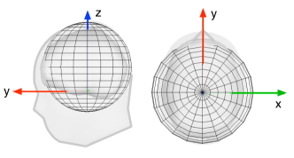
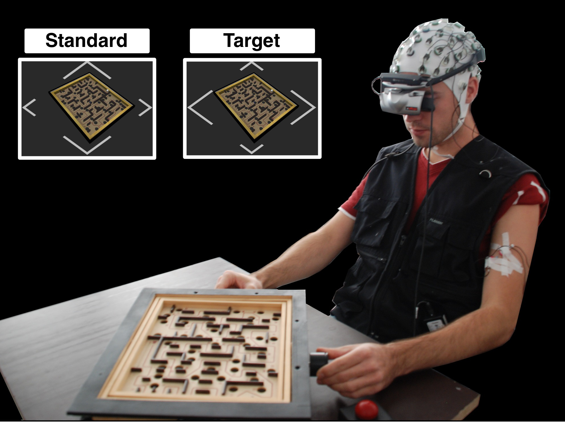
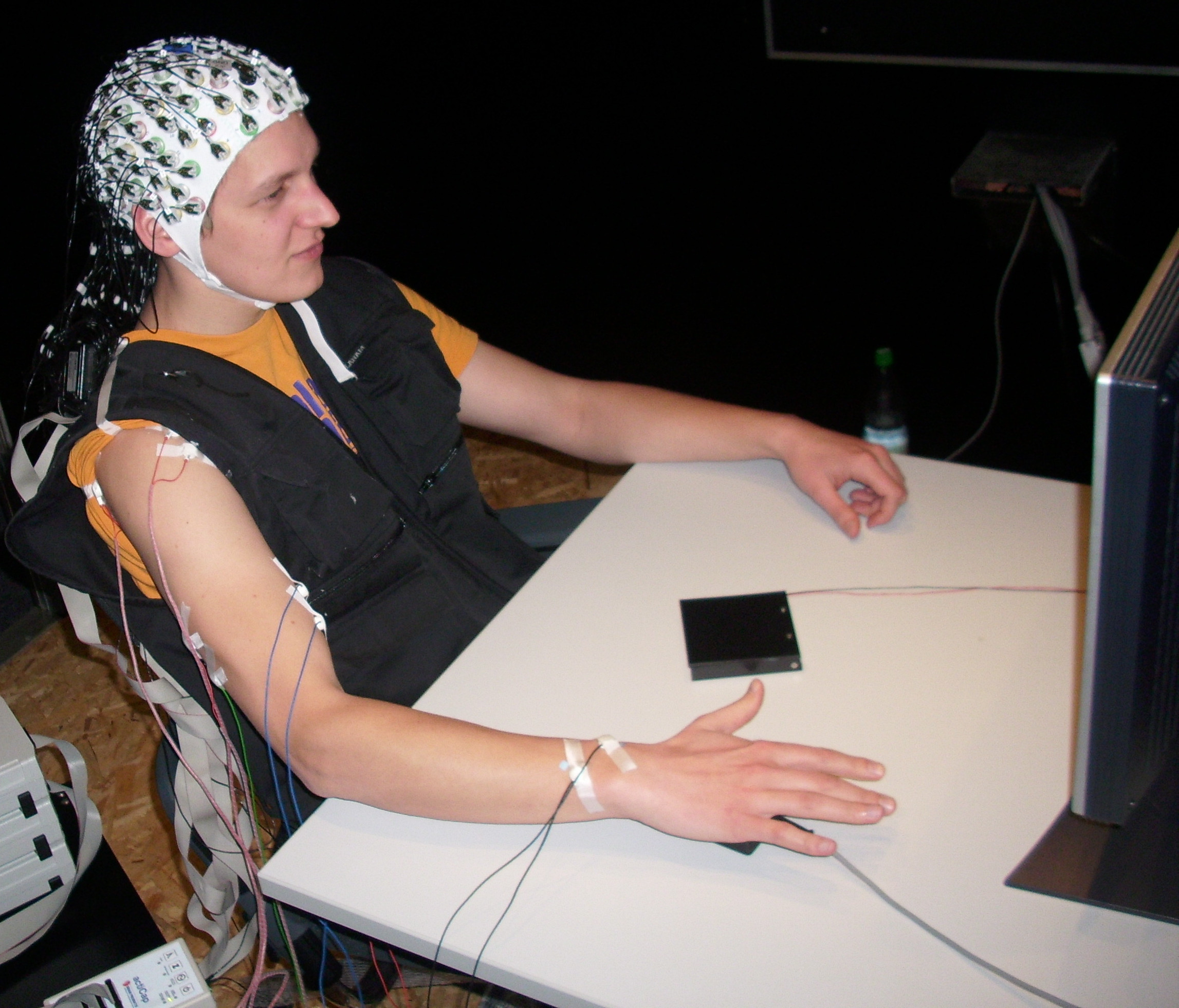
Figure 1: [left] Spherical head model – The x-axis points to the right, the y-axis to the front, and the z-axis runs through the vertex. [middle] Recording setup P300 dataset – The subject plays a virtual Labyrinth game and reacts to the target stimuli with larger left and right corner by pressing the buzzer [17]. [right] Recording setup MRCP dataset [39] – The subject moves his/her hand voluntarily from a switch to a buzzer while he/she sees a fixation cross on a monitor.

2.3 Temporal distortions

In most cases, EEG classification deals with the detection of cognitive processes, which are triggered by events that occur at specific time points. For P300 classification, there are two different events: a) rare occurring task-relevant events (targets) and b) more frequently occurring task-irrelevant events (non-targets). Around $300$ ms after its presentation, the task-relevant event leads to a specific pattern in the brain called P300 [4]. The time point of presentation of an event is marked in the EEG stream (event marker). A common approach is to segment the continuous EEG based on these event markers. Although the event markers are accurate, a latency delay of the P300 can occur for different reasons. For example, it is possible that there is a delay between the display of the events (on the monitor) and the perception of the events, since the subjects have different visual focuses. Workload changes during the experiment can also lead to a latency delay of the P300 [19] and amplitude changes (e.g., a reduction of the P300 amplitude [18]). Note that the processing is usually resistant to different amplitudes (scaling) of the pattern due to the aforementioned data standardization.

Another example of ERP classification is movement prediction based on movement-related cortical potentials (MRCPs) (e.g., [1, 33, 5]). MRCPs include pre-movement components that mainly reflect preparatory processes of the brain before a movement [35]. Since the preparation is a covert process where its onset in single-trial is unknown [38], the event that can be marked in the EEG is just the movement onset. Further, there is not even a perfect estimate on when the movement starts, since usually the time point of the event has to be extracted from a different data stream and is not given by the experiment. So using different data segments that are shifted in time is promising here, too.

For data augmentation of EEG data, it might be also possible to stretch or compress the signal as it is common for image data. This would be for example appropriate, when the pattern of an ERP is expected to change in its length but not its latency. Adding random noise to the data is not a good idea, because the data already has a very low signal to noise ratio in contrast to image data. If frequency changes were expected in the data, the frequency domain of the time signal should be taken into consideration and shifts or distortions should be performed in it [8]. Also, if there is no real triggering event but a certain condition over time (e.g., imagining movements), sliding windows could be used to cut out data segments from the data [31].

To keep the processing load for our evaluation low, we focus on shifting the marker of the triggering event. This can be easily accomplished by cutting out additional segments according to artificially shifted event markers (Details, see Section 3.3).

3 Evaluation

In this section, both spatial and temporal data augmentation approaches were evaluated on the P300 and the MRCP data (Section 3.1). In Section 3.2, we analyzed different parameters and properties of the rotational distortion. In Section 3.3, the aspect of shifting the phase was evaluated. All data processing was performed with the open-source signal processing and classification environment pySPACE [21] on a high performance cluster.

3.1 Dataset, Preprocessing, Classification

For our experiments we used an initial simple setting on P300 data and for the statistical evaluation, we analyzed the transfer between subjects for P300 as well as for MRCP data.

The experimental scenario for P300 data (displayed in Figure 1[middle]) is based on an oddball paradigm (for details see, Kirchner et al. [17] and the appendix, Section B). Here, we used the recorded EEG data from $5$ subjects. Two recording sessions were collected per subject on two different days. Each session consisted of five runs and each run contained $720$ standards and $120$ targets. We first analyzed the transfer between different recording days (inter-session) on P300 data (sample size $10$) and for statistical analysis we used the transfer between sessions of different subjects (sample size $80$ due to more possible combinations). For movement prediction based on MRCPs, data from $8$ subjects performing voluntary arm movements with $3$ different speeds was used (for details see [39], the appendix, Section C, and Figure 1[right]). For every speed condition, three runs each containing $40$ movements were collected. We merged all datasets of a subject and analyzed again the transfer between subjects. Both studies were approved by the ethic committee of the University of Bremen.

For processing, we used classical pipelines [17, 32] consisting of stream segmentation, standardization, downsampling, FFT frequency filter, xDAWN spatial filter, local straight line features, a linear support vector machine (SVM) [7] with 2x5-fold cross-validation for hyperparameter optimization, and a threshold optimization to adapt the decision boundary to the chosen metric (details see the appendix, Sections D and E). The rotational data augmentation was applied directly before the spatial filter. To account for the unbalanced class ratio, we use the balanced accuracy as performance metric, which is the arithmetic mean of true positive and true negative rate [37].

3.2 Rotational Data Augmentation

Before we evaluated our data augmentation approaches, we investigated the general effect of rotating the cap positions on classification performance. Here, no data augmentation was applied (Section 3.2.1). We analyze the effect of different rotation axes (Section 3.2.2) and changes of data dimensions on classification performance (Section 3.2.3).

Eventually, the core results are investigated with statistical verification on subject transfer setups on the two different datasets. For all cases, the effect of different rotation angles on classification performance was considered.

3.2.1 Cap Shifts

One idea underlying spatial robustness is based on the common knowledge: a) The electrodes can be shifted during the recording session and b) The electrode positions will be usually different between recording sessions (i.e., different recording days with the same subject). The shift of electrode positions can be greater between subjects. Thus, the effect of shift of electrode positions on classification performance can be revealed within the same session and such effect will be even stronger in the transfer between sessions and subjects.

In this evaluation, we visualized the effect of shifted electrode positions and determine whether our interpolation method (details, see Section 2.2) is capable of compensating for the shift of electrode positions. Here, the data was not augmented but the original training data was replaced with a rotation around a single axis. The testing data was kept the same. The expected shape would be a perfect bell curve, centered around zero. For the different axes, the classification performances are depicted in Figure 2 for cap shifts with different angles except for the x-axis where no relevant effect could be observed. For the y-axis, a deviation from optimum at an angle of zero can be observed in $7$ out of $10$ cases. When the train and test data are exchanged, the deviations from the zero angle should be reversely mirrored. Such opposite pattern are apparent for subject 3 and subject 4. For the z-axis, all subjects showed deviations and the opposite pattern except for one subject. Especially, the opposite pattern was obviously visible for subject 6. All relevant angle shifts were between $-4$\mathrm{\SIUnitSymbolDegree}$$ to $6$\mathrm{\SIUnitSymbolDegree}$$.

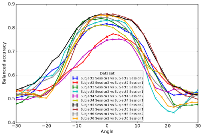
Figure 2: Cap shift with different angles for a single axis (left: y-axis, right: z-axis) in the setting of transfer between sessions. No relevant effect for the x-axis could be observed.

Altogether, this indicates that cap shifts occurred between $-4$\mathrm{\SIUnitSymbolDegree}$$ to $6$\mathrm{\SIUnitSymbolDegree}$$ and can be (at least partially) compensated with our approach, although other factors also seem to have an influence. Furthermore, we can see that the influence is largest on the z-axis, followed by the y-axis, and it is probably irrelevant on the x-axis. This effect was further analyzed in the next section together with the data augmentation.

3.2.2 Rotation Axes

In this section, we analyze the effect of the three rotation axes in the data augmentation for P300 data. Here, we evaluate both single axis data and possible axes combinations. For the data augmentation, we took the original data and added an artificial sample for the chosen angle in positive and negative direction.

Using the x-axis reduces performance on average, whereas the augmentation around the y- and z-axis increases performance, in which the z-axis slightly outperforms the y-axis (for details we refer to the appendix, Section H). This is consistent with the observation in Section 3.2.1 that the z-axis has the largest effect of cap shifts and the x-axis is not affected by it. The combination of y- and z-axis slightly increases classification performance, whereas adding data, augmented with a rotation around the x-axis, decreases classification performance in every combination.

The best performance was achieved with an angle between $12$\mathrm{\SIUnitSymbolDegree}$$ and $24$\mathrm{\SIUnitSymbolDegree}$$ over all subjects. This pattern is different from the evaluation of a single axis, in which the much smaller angles were relevant for the cap shifts (see Section 3.2.1). A possible reason is that the classifier interpolates for the angles in-between or generalizes better with this larger difference of the angles.

We also looked at the variability between subjects in the performance (see also the appendix, Section H) Such subject-specific performance should be considered, since we aim to configure the data augmentation as independent from data properties as possible. We observed a performance increase in $5$ out of $10$ cases. In the other cases, there is no change or a slight decrease. This absence of a substantial decrease is very important for the applicability of our approach.

3.2.3 Data Reduction and Data Dimensionality Increase

In general, the dimensionality correlates with the cap configuration (i.e., cap with different numbers of electrodes). It is well known that machine learning algorithms behave differently depending on the ratio between dimension of the data after the preprocessing and number of provided samples for each class. For the xDAWN in the processing chain, the use of a larger number of filters increases data dimension for the SVM classifier. For the case of using small rotation angles, the performance was reduced due to an increased feature dimension (see Figure 3 [left]). For $16$ filters, the dimension is doubled, and for $32$ it is quadrupled. Fortunately, it is not relevant for larger angles over $14$\mathrm{\SIUnitSymbolDegree}$$ (statistic details in the appendix, Section I). This is very positive for our augmentation strategy because it is still applicable when there is a lack of data. The reason for the performance drop for small angles is probably that the data augmentation is modeled by the classifier as noise and degrades the classifier model whereas larger angles are modeled like new data.

Figure 3 [right] shows a similar effect when reducing the data size. Again, there is a performance drop for small angels when $20\%$ or $40\%$ of the data is used, but still the performance is increased for rotation augmentation between $18$\mathrm{\SIUnitSymbolDegree}$$ and $20$\mathrm{\SIUnitSymbolDegree}$$(statistic details in the appendix, Section I). The overall performance is decreased due to the reduction of data size, which is expected. Note that the performance drop for small angles was not shown when sufficient amounts of data are available ($60\%$, $100\%$).

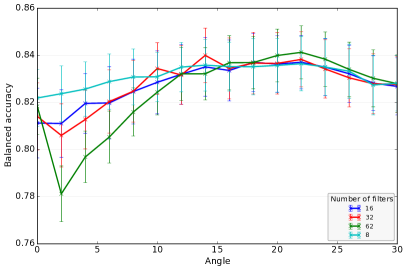
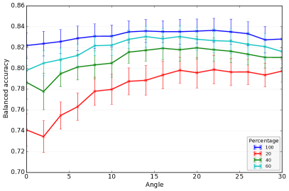
Figure 3: Comparison with different increased dimensionality (number of spatial filters – left) and data reduction (percentage of used training data – right).

3.2.4 Subject Transfer

In this section, we investigated our rotational data augmentation approach for the more challenging transfer setting between subjects with statistical verification. In this transfer setting, we obtained $80$ performance values (sample size of $80$): for each of the $5$ subjects, there were $2$ sessions for training, which each were combined with testing on the data of the other $4$ subjects with $2$ sessions ($5$ subjects $\cdot$ $2$ sessions $\cdot$ $4$ subjects $\cdot$ $2$ sessions) for P300 data. We obtained $56$ performance values (sample size of $56$) for MRCP data: $8$ training datasets from the $8$ subjects combined with each of the remaining $7$ datasets for testing. For the comparison between different axes (x, y, z) and their combination (y, z) in different angles, we performed a two-way repeated measures ANOVA with axis and angel as within-subjects factors. Note that we only combined y and z based on the previous evaluation on the session-transfer setting. For the comparison between interpolation strategies in different angles, we performed a two-way repeated measures ANOVA with interpolation strategy and angel as within-subjects factors. For multiple comparisons, Bonferroni-Holm was applied. Hence, we correct for multiple testing on the same dataset.

In Figure 4[left], we compared different axes (with the “cubic” parameter for the interpolation function according to the previous evaluation in the appendix, Section G). The performance is clearly affected by the axes [$F_{3,237}$ = $23.9$, $p<0.001$]. Again, the z-axis has the largest impact on the performance across angles [$z$ vs. $y$: $p<0.003$, $z$ vs. $x$: $p<0.002$] but this time the combination with the y-axis does not further improve the performance over all angles [$z$ vs. $z,y$: $p=n.s.$]. The overall performance is reduced due to the more difficult transfer setting (transfer between subjects) but rotations with an angle between $18$\mathrm{\SIUnitSymbolDegree}$$ and $26$\mathrm{\SIUnitSymbolDegree}$$ shows an increase in performance as beforehand [rotation effect: $F_{15,1185}$ = $5.50$, $p<0.001$, interaction effect: $F_{45,3555}$ = $1.07$, $p=n.s.$, no rotation ($0$\mathrm{\SIUnitSymbolDegree}$$) vs. between $18$\mathrm{\SIUnitSymbolDegree}$$ and $26$\mathrm{\SIUnitSymbolDegree}$$: $p<0.05$, between $2$\mathrm{\SIUnitSymbolDegree}$$ and $4$\mathrm{\SIUnitSymbolDegree}$$ vs. between $18$\mathrm{\SIUnitSymbolDegree}$$ and $26$\mathrm{\SIUnitSymbolDegree}$$: $p<0.05$] for z-axis and axis combination of z and y. In Figure 5[left], we compared different interpolation strategies while rotating around the y- and z-axes. All interpolation methods have a similar performance [interpolation effect: $F_{5,395}$ = $5.50$, $p=n.s.$,]. Again, the performance increases with rotations with an angle between $18$\mathrm{\SIUnitSymbolDegree}$$ and $26$\mathrm{\SIUnitSymbolDegree}$$ except for multiquadric and gaussian [no rotation ($0$\mathrm{\SIUnitSymbolDegree}$$) vs. between $18$\mathrm{\SIUnitSymbolDegree}$$ and $26$\mathrm{\SIUnitSymbolDegree}$$: $p<0.05$].

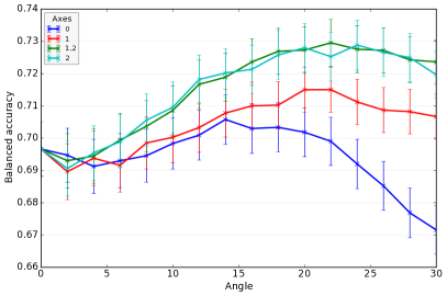
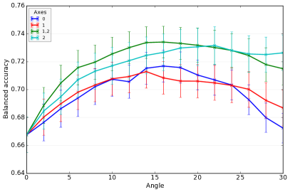
Figure 4: Data augmentation with a rotation around the different axes: x (0), y (1), z (2). For the training the original data is taken and the augmented data with a rotation angle of +angle and -angle is added. This triples the amount of data and in case of combining the augmented data by rotating around y and z (1,2) it is $5$ times the original data. An angle of $0$ corresponds to the baseline with no augmentation. See also Figure 1 for the meaning of the axes. For testing no data augmentation was applied. [left] Subject transfer P300 data. [right] Subject transfer MRCP data.

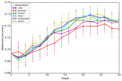
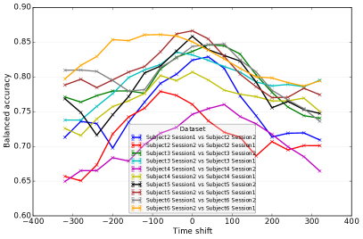
Figure 5: [left] Data augmentation with rotation around the z- and the y-axis for different interpolation parameters (P300 subject transfer) where $0$ corresponds to no augmentation. [right] Comparison of different time shifts (in milliseconds) (P300 session transfer).

We obtained a similar results on MRCP data as P300 data. Figure 4[right] shows an effect of the rotation angle on classification performance [$F_{3,165}=15.02,p<0.001$]. Again, the z-axis achieves a better performance compared to x- and y-axis [$z$ vs. $x$: $p<0.001$, $z$ vs. $y$: $p<0.002$]. Performance improvements through the axis combination is not observed as P300 data. [$z$ vs. $z,y$: $p=n.s.$]. Further, improvements through rotations with an angle is observed both for z-axis and axis combination of z and y between $16$ and $30$ and between $10$ and $24$ respectively [no rotation ($0$\mathrm{\SIUnitSymbolDegree}$$) vs. between $16$\mathrm{\SIUnitSymbolDegree}$$ and $30$\mathrm{\SIUnitSymbolDegree}$$: $p<0.03$ for z-axis, no rotation ($0$\mathrm{\SIUnitSymbolDegree}$$) vs. between $10$\mathrm{\SIUnitSymbolDegree}$$ and $24$\mathrm{\SIUnitSymbolDegree}$$: $p<0.04$ for z,y-axis].

3.3 Time shift

In this section, we did not analyze spatial but temporal shifts. The preprocessing was exactly the same but when cutting out segments, different offsets were used to generate shifted data. Similar to Section 3.2.1, we first analyzed the effect of the time shift on the classification performance. Second, we augmented the data by adding data with positive and/or negative offset to the data with zero offset.

For P300 data, using data with a non-zero offset slightly improved performance for individual subjects (Figure 5[right]) which is reasonable due to the arguments in Section 2.3. Furthermore, a change in the sign of the optimal time shifts was observed when comparing two sessions. On average, performance decreased when the original zero offset was not used.

The results did not show a clear favoring time for augmentation that holds for all subjects. Hence, we tested the augmentation with positive and negative time together. Adding data with $40$ and $-40$ ms shift ($3$ times the training data) did not change performance on average but using larger offsets decreased performance (see also the appendix, Section F). Hence, this approach does not add temporal robustness in our case (P300 detection) but at least increases the number of samples.

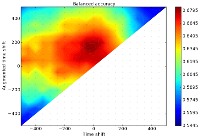
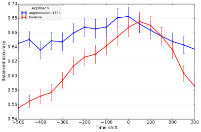
Figure 6: Subject transfer MRCP data. [left] Classification performance of augmentation through combined time shifts (in milliseconds) depending on an initial time shift. [right] Comparison of different single time shifts (red) and augmented time shift of $150$ ms (blue) depending on the initial time shift. Note, for the testing data neither initial nor augmented time shift was applied.

For the investigation of the effect of augmentation through time shift for the MRCP data, we performed a two-way repeated measures ANOVA with time shift and augmentation as within-subjects factors. For multiple comparisons, Bonferroni-Holm was applied. Figure 6[left] shows the classification performance when the training data used to detect movement preparation was augmented by a time shift. The diagonal represents the baseline where only a single time was used for training the classifier (i.e., no augmentation equivalent to red line in Figure 6[right]). The highest classification performance was not observed on the diagonal but with a time shift of $+150$ ms, i.e., augmentation improves the performance (blue line in Figure 6[right]). Obviously, both augmentation and time shift had an impact on the performance (Figure 6[right]) [augmentation effect: $F_{1,55}=55.06,p<0.001$, time shift effect: $F_{8,440}=11.14,p<0.001$]. Considering the results without an initial time shift (time shift $0$ ms), we observed performance improvement through data augmentation with a time shift of $150$ ms [baseline vs. augmentation: $p<0.05$]. In comparison to the rotational augmentation, the increase in performance through time augmentation was smaller ($6$ % vs $1$ %). A possible explanation could be the subject transfer setting: best time shifts and best time shift combinations through augmentation might be subject specific.

4 Conclusion

In this paper, we proposed several data augmentation techniques for EEG data to generate new data without reducing the performance. We analyzed and compared the behavior of these on real EEG data for P300 detection and movement prediction (MRCP data). Our analyses showed that the data augmentation did not substantially reduce the performance on average with appropriately chosen configurations. In particular, concerning rotational shifts, we showed a significant increase of classification performance with a general setting of rotating only around the z-axis with an angle around $18$ degrees. Additionally, we obtained significant improvements on MRCP data with a temporal shift.

In future, we want to analyze further augmentation strategies, use our findings for deep learning, and evaluate it on other paradigms. Furthermore, it would be interesting to investigate whether complex head models or aggregation of augmented results to one decision can improve the performance further.

Appendix A Structure of EEG Data and How to Obtain 2D-Representations of 3D Sensor Positions

EEG data can be seen as two-, three-, or four-dimensional data. The temporal dimension/axis is the most important one, because the data comes with a very high resolution of up to $5$kHZ that is directly related to the current brain activity. Usually a maximum of $100$Hz is needed for data analysis. Hence, it is common to standardize the data, reduce the frequency range at least to less than $100$Hz and remove slow drifts which can for example result from conductivity changes by sweating.

There are, of course, approaches that consider the spatial relations between electrodes (e.g, source localization methods [26], connectivity methods, etc.). However, such methods require a considerable amount of expert knowledge and computational power compared to the classical BCI applications. Correlations between electrode measurements are considered by dimensionality reduction algorithms like spatial filters without considering the real positions.

It is also possible to map the electrodes to a rectangular 2D-shape to enable a spatial convolution instead or additionally to a spatial filter layer in deep learning as outlined in the following.

For obtaining 2D coordinates that correspond to the true 3D positions, there are three different methods. Given the spherical coordinates $(r,\phi,\theta)$, one possible mapping is x = r2 * numpy.cos(theta) * 60, y = r2 * numpy.sin(theta) * 60 with r2 = r / numpy.power(numpy.cos(phi), 0.2). This representation is very common for plots of the signal but not that useful for convolutional filter even though the resulting visualizations could be used for applying standard image CNNs [2].

But it is also possible to map the electrodes by hand to a rectangular shape (see Table 1). Note, that this mapping is targeting a specific selection of sensors. For a more general setting with arbitrary types of homogeneous sensors an identification algorithm by Kampmann [13](section 5.1.6) can be used. First, a graph is constructed by the similarity between sensors (like distance or covariance) and rearranged by the force-directed layout algorithm to have neighboring sensors to be also nearby in the 2D graph representation. For the final mapping of the graph to a rectangular shape, self-organizing map are used.

Table 1: 2D rectangular mapping of EEG electrode positions.

F7	AF7	FP1	AF3	Fz	AF4	FP2	AF8	F8
FT9	F5	F3	F1	FCz	F2	F4	F6	FT10
FT7	FC5	FC3	FC1	Cz	FC2	FC4	FC6	FT8
T7	C5	C3	C1	CPz	C2	C4	C6	T8
TP9	CP5	CP3	CP1	Pz	CP2	CP4	CP6	TP10
P7	P5	P3	P1	POz	P2	P4	P6	P8
PO9	PO7	O1	PO3	Oz	PO4	O2	PO8	PO10

Appendix B P300 Data

In the experimental scenario, the subject saw a task-irrelevant event (standard) every second with a latency jitter of $\pm 100$ ms. With a probability of $1/6$, a task-relevant event (target) was randomly displayed. The task relevant event/stimulus required a reaction from the subject (see also Figure 1[middle]). The stimuli were chosen to be very similar to avoid the effect of color or shape on the brain pattern. Based on this reaction to the targets, we can infer the true label for standards and targets. When the subject correctly responded to targets, we can ensure that targets were correctly perceived. The perceived task-relevant event leads to a specific pattern in the brain, called P300. In this scenario, the continuous EEG was recorded from $5$ subjects using a 64 channel actiCap system (Brain Products GmbH, Munich, Germany) with reference at FCz (extended 10-20 system). Two electrodes of the 64 channel system were used to record the electromyogram (EMG) which is related with to pressing of the buzzer. Impedance was kept below $5$ k$\Omega$. EEG and EMG signals were sampled at $1$ kHz, amplified by two 32 channel BrainAmp DC amplifiers (Brain Products GmbH, Munich, Germany) and filtered with a low cut-off of $0.1$ Hz and high cut-off of $1$ kHz. Two recording sessions were collected per subject on two different days. Each session consists of five runs and each run contains $720$ standards and $120$ targets. Targets without a response by the subject were not considered in our evaluation. The motivation of the previous study by Kirchner et al. [17] was to transfer the trained classified to distinguish missed and perceived targets by treating missed targets like standards due to similarities in the shape. Hence, a few of the provided trials (missed targets) had to be removed because no clear label could be assigned. We first analyzed the transfer between different recording days (inter-session) on P300 data and for statistical analysis we used the transfer between sessions of different subjects.

Appendix C MRCP Data

Eight healthy, right-handed male subjects took part in the experiment where they performed self-initiated movements. Subjects sat in a comfortable chair in a dimly lit room, resting their arms on a table in front of them. Subjects placed their hand on a flat switch and saw a fixation cross presented on a monitor (see also Figure 1[right]). A buzzer was placed approximately $20$ cm to the right from the switch. Subjects could initiate whenever they want a movement from the switch to the buzzer but a resting time of at least $5$ s between consecutive movements had to be maintained. Subjects were informed on the monitor if they violated that condition and the performed movement was marked as invalid. Invalid trials were not considered in data analysis. Each experimental run consisted of $40$ valid movements. For each condition, e.g. different speeds, three runs were recorded. Subjects were first instructed to perform the movements in their normal speed. The subject performed fast and slow movements according to predefined speed restriction, which was individually calculated per subject.

EEG data was recorded with actiCAP ($128$ electrodes placed according to the extended 10-20 scheme) and four BrainAmp DC amplifiers (all Brain Products GmbH, Munich, Germany). FCz was used as reference and impedances were kept below $5$ k$\Omega$. Before storing the data with a sampling frequency of $5$ kHz to disk, a band-pass filter between $0.1$ und $1000$ Hz was applied. The start and end of a movement was marked into the EEG stream based on events from the switch and buzzer, respectively.

Appendix D P300 Preprocessing

We segmented the continuous EEG based on each event with a segment length of one second and normalized them to zero mean and a standard deviation of one. The sampling rate of the data was reduced from $1000$Hz to $25$Hz. Then the data was low-pass filtered with a cut-off frequency of $4$Hz, which was chosen based on our previous evaluations.

After this preprocessing step, the data augmentation approaches were applied except of the temporal shifts. Those were already applied at the beginning of the processing chain during the cutting of the segments. Next, the xDAWN spatial filter [30] was trained on the complete training data and then applied. Afterwards, local straight lines were fitted and the respective slopes were taken as features. Features were normalized to zero-mean and unit-variance on the training data. The used classifier was a standard (affine) SVM implementation with a linear kernel [7] and limited number of iterations ($100$ times the number of samples). The regularization hyperparameter $C$ of the SVM was optimized using $5$ fold cross validation with two repetitions and with the values $[10^{0},10^{-0.5},\ldots,10^{-4}]$. Eventually, a threshold optimization was applied.

For an inter-session P300 evaluation, we train with the data of one recording session and then test on the other remaining recording session of the same subject. This results in $10$ samples ($5$ subjects * $2$ sessions). Setting the cap anew at this other day, can result in slight changes of the electrode positions. For an inter-subject P300 evaluation, we train with the data of one recording session and then test on the recording sessions of the remaining subjects. This results in $80$ samples ($5$ subjects * $2$ sessions * $4$ subjects * $2$ sessions).

Appendix E MRCP Preprocessing

We segmented the continuous EEG based on the switch event (switch release). Since event has some delay in detecting the actual movement onset, we used a window of one second length ending $100$ ms before the switch event. In this way we could ensure that the upcoming movement is predicted and not just detected. For the opposite class, we cut out non-overlapping windows starting soonest $1$ s after subjects entered the switch and ended latest $0.8$ s before subjects left the switch. For the time augmentation we varied the end time of the windows for the movement preparation class between $-0.6$ to $+0.5$ s with respect to the switch release.

First, the data was normalized channel-wise to zero mean and unit variance. Next, a decimation from $5$ kHz to $20$ Hz was performed in two steps. Then, the data was band-pass filtered between $0.1$ and $4$ Hz using a FFT. Subsequently the data was reduced to the last $200$ ms since the most relevant information is expected in that range. At this point the rotational data augmentation was applied in our analysis. Afterwards the xDAWN spatial filter [30] was trained which reduced the dimension of the data to $4$ pseudo-channels. These were directly used as features ($4$ channels $\times$ $4$ time points $=16$ features), normalized (zero-mean, unit-variance) and passed to a standard (affine) SVM implementation with a linear kernel [7] and limited number of iterations ($100$ times the number of samples). The regularization hyperparameter $C$ of the SVM was optimized using $5$ fold cross validation with two repetitions and with the values $[10^{0},10^{-1},\ldots,10^{-6}]$. To account for the class imbalance a class weight of $2$ was used inside the SVM. Finally a threshold optimization was performed to adapt the decision boundary to the chosen performance metric, i.e., the balanced accuracy.

Appendix F Temporal Distortions P300

The results for the temporal are depicted in Figure F.7. Here, zero was not the best choice for the offset which is reasonable due to possible changes of the P300 offset between experiments. Furthermore, a change in the sign of the optimal time shifts was observed when comparing two sessions which strengthens the impression that this a systematic effect. On average, performance decreased when the original zero offset was not used. But for the data augmentation, adding data with $40$ and $-40$ ms shift did not change performance on average but using larger offsets decreased performance. Hence, this approach does not add temporal robustness in our case (P300 detection) but at least increases the number of samples.

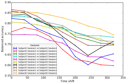
Figure F.7: Data augmentation through time shift in milliseconds in the setting of transfer between sessions. [left] Augmentation with one time shift additionally to the original data ($0$). [right] Augmentation with two time shifts: $\pm$ time shift additionally to the original data.

Appendix G Interpolation Strategy

For the interpolation, different strategies could be used in SciPy. In a preliminary analysis on synthetic data, we found out that the scipy.interpolate.Rbf library fits best to our research issue. Due to the 3-dimensional positioning of the electrodes, the interpolation is not straightforward. Different parameters can be used for an internal modeling function. So far, we used the default strategy (“multiquadric”). As shown for Figure G.8 [left], the default method performed quite well but slightly better results might be achieved with another interpolation function like “quintic” or “cubic”.

Further, we evaluated whether the data augmentation/interpolation is possible for smaller electrode constellations ($32$ and $19$ electrodes according to the $10$-$20$ system). This evaluation shows that the data augmentation did not reduce the performance for smaller electrode constellation, but there was also no relevant improvement between angles (see Figure G.8 [right]). This indicates that the interpolation is not good enough if the electrodes are positioned too sparse.

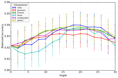
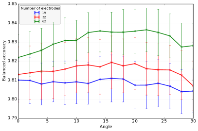
Figure G.8: Comparison of interpolation strategies (left) and different cap configurations containing a different number of electrodes (right).

Appendix H Comparison of Rotation Axes for Inter-Session Evaluation on P300 Data

Figure H.9 depicts the result for the comparison on the inter-session evaluation on P300 data for the comparison different axes as well as the individual results for the case of rotating around z- and the y-axis.

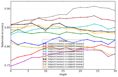
Figure H.9: Data augmentation with a rotation around the different axes: x (0), y (1), z (2) and a rotation angle of +angle and -angle (combined). For the left image, the augmented data of the different rotation axes is combined for training. The right picture shows the data augmentation with rotation around the z- and the y-axis (corresponds to “1,2”) for each session transfer.

Appendix I Statistical evaluation

In regards to Section 3.2.3 Data Reduction and Data Dimensionality Increase: For comparison between different number of filters and rotation angles (Figure 3 [left]), we performed a two-way ANOVA with number of filters and rotation angle as within-subjects factors. For multiple comparisons, Bonferroni-Holm was applied. Rotation angle has an effect on the classification performance [$F_{15,135}=2.53,p<0.031$,], but the number of filters does not [$F_{3,27}=0.96,p=n.s.$]. We observe the performance decrease for small rotation angles ($2$\mathrm{\SIUnitSymbolDegree}$$), but this performance reduction recovers when increasing rotation angles (between $14$\mathrm{\SIUnitSymbolDegree}$$ and $20$\mathrm{\SIUnitSymbolDegree}$$). This pattern is obviously revealed for large data dimension (filter number of $64$) [$2$\mathrm{\SIUnitSymbolDegree}$$ vs. between $14$\mathrm{\SIUnitSymbolDegree}$$ and $20$\mathrm{\SIUnitSymbolDegree}$$: $p<0.05$].

For comparison between training sizes and rotation angels (Figure 3 [right]), we performed a two-way ANOVA with training size and rotation angle as within-subjects factors. For multiple comparisons, Bonferroni-Holm was applied. Both training size and rotation angels have an effect on the classification performance [effect of training size: $F_{3,27}=66.99,p<0.001$, effect of rotation angel: $F_{15,135}=3.52,p<0.001$]. We found no interaction effect between both factors [$F_{45,405}=0.41,p=n.s.$]. Especially, performance increase through rotation is observed between $18$\mathrm{\SIUnitSymbolDegree}$$ and $20$\mathrm{\SIUnitSymbolDegree}$$ [no rotation ($0$\mathrm{\SIUnitSymbolDegree}$$) vs. between $18$\mathrm{\SIUnitSymbolDegree}$$ and $20$\mathrm{\SIUnitSymbolDegree}$$: $p<0.05$]. This kind of performance improvement is particularly revealed for the training size of $20\%$, i.e., a significant effect of rotation angle is only revealed when the training size is small. A statistic with significant effects with larger training size is provided for the subject transfer setting (Section 3.2.4). For the transfer between P300 recording sessions, the sample size was only $10$ in contrast to $80$ and $56$ for the other comparisons.

References

- [1] O. Bai, V. Rathi, P. Lin, D. Huang, H. Battapady, D.-Y. Fei, L. Schneider, E. Houdayer, X. Chen, and M. Hallett. Prediction of human voluntary movement before it occurs. Clinical Neurophysiology, 122(2):364–372, Feb. 2011.
- [2] P. Bashivan, I. Rish, M. Yeasin, and N. Codella. Learning Representations from EEG with Deep Recurrent-Convolutional Neural Networks. nov 2016.
- [3] B. Blankertz, G. Dornhege, S. Lemm, M. Krauledat, G. Curio, and K.-R. Müller. The Berlin Brain-Computer Interface: Machine Learning Based Detection of User Specific Brain States. Journal of Universal Computer Science, 12(6):581–607, 2006.
- [4] E. Courchesne, S. A. Hillyard, and R. Y. Courchesne. P3 Waves to the Discrimination of Targets in Homogeneous and Heterogeneous Stimulus Sequences. Psychophysiology, 14(6):590–597, nov 1977.
- [5] R. Darmakusuma, A. S. Prihatmanto, A. Indrayanto, T. L. Mengko, L. A. Andarini, and A. F. Idrus. Analysis of Arm Movement Prediction by Using the Electroencephalography Signal. Makara Journal of Technology, 20(1):38–44, 2016.
- [6] S. A. Hillyard and M. Kutas. Electrophysiology of cognitive processing. Annual review of psychology, 34(1):33–61, 1983.
- [7] C.-J. Hsieh, K.-W. Chang, C.-J. Lin, S. S. Keerthi, and S. Sundararajan. A dual coordinate descent method for large-scale linear SVM. In Proceedings of the 25th International Conference on Machine learning (ICML 2008), pages 408–415. ACM Press, jul 2008.
- [8] Huijuan Yang, S. Sakhavi, Kai Keng Ang, and Cuntai Guan. On the use of convolutional neural networks and augmented CSP features for multi-class motor imagery of EEG signals classification. In 2015 37th Annual International Conference of the IEEE Engineering in Medicine and Biology Society (EMBC), pages 2620–2623. IEEE, aug 2015.
- [9] P. jan Kindermans, H. Verschore, D. Verstraeten, and B. Schrauwen. A p300 bci for the masses: Prior information enables instant unsupervised spelling. In F. Pereira, C. J. C. Burges, L. Bottou, and K. Q. Weinberger, editors, Advances in Neural Information Processing Systems 25, pages 710–718. Curran Associates, Inc., 2012.
- [10] V. Jayaram, M. Alamgir, Y. Altun, B. Scholkopf, and M. Grosse-Wentrup. Transfer learning in brain-computer interfaces. IEEE Computational Intelligence Magazine, 11(1):20–31, Feb 2016.
- [11] E. Jones, T. Oliphant, P. Peterson, and Others. SciPy: Open source scientific tools for Python, 2001.
- [12] E. Kalunga, S. Chevallier, and Q. Barthélemy. Data augmentation in riemannian space for brain-computer interfaces. In ICML Workshop on Statistics, Machine Learning and Neuroscience (Stamlins 2015), 2015.
- [13] P. Kampmann. Development of a multi-modal tactile force sensing system for deep-sea applications. Phd thesis, University of Bremen, Bremen, 2016.
- [14] P.-J. Kindermans, M. Tangermann, K.-R. Müller, and B. Schrauwen. Integrating dynamic stopping, transfer learning and language models in an adaptive zero-training erp speller. Journal of Neural Engineering, 11(3):035005, 2014.
- [15] E. A. Kirchner. Embedded Brain Reading. PhD thesis, Universität Bremen, 2014.
- [16] E. A. Kirchner, J. Albiez, A. Seeland, M. Jordan, and F. Kirchner. Towards assistive robotics for home rehabilitation. In M. F. Chimeno, J. Solé-Casals, A. Fred, and H. Gamboa, editors, Proceedings of the 6th International Conference on Biomedical Electronics and Devices (BIODEVICES-13), pages 168–177, Barcelona, Feb 2013. ScitePress.
- [17] E. A. Kirchner, S. K. Kim, S. Straube, A. Seeland, H. Wöhrle, M. M. Krell, M. Tabie, and M. Fahle. On the applicability of brain reading for predictive human-machine interfaces in robotics. PloS ONE, 8(12):e81732, jan 2013.
- [18] E. A. Kirchner, S. K. Kim, M. Tabie, H. Woehrle, M. Maurus, and F. Kirchner. An intelligent man-machine interface - multi-robot control adapted for task engagement based on single-trial detectability of p300. Frontiers in Human Neuroscience, 10(291), 2016.
- [19] A. Kok. On the utility of p3 amplitude as a measure of processing capacity. Psychophysiology, 38(3):557–577, 2001.
- [20] M. M. Krell and S. K. Kim. Rotational data augmentation for electroencephalographic data. In 2017 39th Annual International Conference of the IEEE Engineering in Medicine and Biology Society (EMBC), pages 471–474. IEEE, jul 2017.
- [21] M. M. Krell, S. Straube, A. Seeland, H. Wöhrle, J. Teiwes, J. H. Metzen, E. A. Kirchner, and F. Kirchner. pySPACE — a signal processing and classification environment in Python. Frontiers in Neuroinformatics, 7(40):1–11, dec 2013.
- [22] A. Krizhevsky, I. Sutskever, and G. E. Hinton. ImageNet Classification with Deep Convolutional Neural Networks. In Advances in Neural Information Processing Systems, pages 1097–1105, 2012.
- [23] F. Lotte. Signal Processing Approaches to Minimize or Suppress Calibration Time in Oscillatory Activity-Based Brain-Computer Interfaces. Proceedings of the IEEE, 103(6):871–890, jun 2015.
- [24] D. J. McFarland, W. A. Sarnacki, and J. R. Wolpaw. Should the parameters of a BCI translation algorithm be continually adapted? Journal of Neuroscience Methods, 199(1):103–107, jul 2011.
- [25] J. H. Metzen, S. K. Kim, and E. A. Kirchner. Minimizing calibration time for brain reading. In R. Mester and M. Felsberg, editors, Pattern Recognition, Lecture Notes in Computer Science, volume 6835, pages 366–375. Springer Berlin Heidelberg, Frankfurt, aug 2011.
- [26] C. M. Michel, M. M. Murray, G. Lantz, S. Gonzalez, L. Spinelli, and R. Grave de Peralta. EEG source imaging. Clinical Neurophysiology: Official Journal of the International Federation of Clinical Neurophysiology, 115(10):2195–2222, Oct. 2004.
- [27] J. d. R. Millán, R. Rupp, G. Müller-Putz, R. Murray-Smith, C. Giugliemma, M. Tangermann, C. Vidaurre, F. Cincotti, A. Kübler, R. Leeb, C. Neuper, K.-R. Müller, and D. Mattia. Combining brain-computer interfaces and assistive technologies: State-of-the-art and challenges. Frontiers in Neuroscience, 4(161), 2010.
- [28] H. Ramoser, J. Müller-Gerking, and G. Pfurtscheller. Optimal spatial filtering of single trial EEG during imagined hand movement. IEEE transactions on rehabilitation engineering : a publication of the IEEE Engineering in Medicine and Biology Society, 8(4):441–6, dec 2000.
- [29] D. Regan. Human brain electrophysiology: evoked potentials and evoked magnetic fields in science and medicine. 1989.
- [30] B. Rivet, A. Souloumiac, V. Attina, and G. Gibert. xDAWN Algorithm to Enhance Evoked Potentials: Application to Brain-Computer Interface. IEEE Transactions on Biomedical Engineering, 56(8):2035–2043, aug 2009.
- [31] R. T. Schirrmeister, J. T. Springenberg, L. D. J. Fiederer, M. Glasstetter, K. Eggensperger, M. Tangermann, F. Hutter, W. Burgard, and T. Ball. Deep learning with convolutional neural networks for brain mapping and decoding of movement-related information from the human EEG. CoRR, abs/1703.05051, 2017.
- [32] A. Seeland, L. Manca, F. Kirchner, and E. A. Kirchner. Spatio-temporal Comparison Between ERD/ERS and MRCP-based Movement Prediction. In A. C. Jr., A. Fred, H. Gamboa, and D. Elias, editors, Proceedings of the 8th International Conference on Bio-inspired Systems and Signal Processing (BIOSIGNALS-15), pages 219–226, Lisbon, Jan 2015. ScitePress.
- [33] A. Seeland, H. Woehrle, S. Straube, and E. A. Kirchner. Online movement prediction in a robotic application scenario. In 6th International IEEE EMBS Conference on Neural Engineering (NER), pages 41–44, San Diego, California, Nov 2013.
- [34] P. Shenoy, M. Krauledat, B. Blankertz, R. P. N. Rao, and K.-R. Müller. Towards adaptive classification for BCI. Journal of Neural Engineering, 3(1):R13–R23, mar 2006.
- [35] H. Shibasaki and M. Hallett. What is the Bereitschaftspotential? Clinical Neurophysiology, 117(11):2341–2356, 2006.
- [36] P. Simard, D. Steinkraus, and J. Platt. Best practices for convolutional neural networks applied to visual document analysis. In Seventh International Conference on Document Analysis and Recognition, 2003, volume 1, pages 958–963. IEEE Comput. Soc, aug 2003.
- [37] S. Straube and M. M. Krell. How to evaluate an agent’s behaviour to infrequent events? – Reliable performance estimation insensitive to class distribution. Frontiers in Computational Neuroscience, 8(43):1–6, jan 2014.
- [38] S. Sur and V. Sinha. Event-related potential: An overview. Industrial psychiatry journal, 18(1):70, 2009.
- [39] M. Tabie and E. A. Kirchner. EMG Onset Detection - Comparison of Different Methods for a Movement Prediction Task based on EMG. In S. Alvarez, J. Solé-Casals, A. Fred, and H. Gamboa, editors, Proceedings of the International Conference on Bio-inspired Systems and Signal Processing, pages 242–247, Barcelona, Spain, feb 2013. SciTePress.
- [40] F. Tadel, S. Baillet, J. C. Mosher, D. Pantazis, and R. M. Leahy. Brainstorm: A User-Friendly Application for MEG/EEG Analysis. Computational Intelligence and Neuroscience, 2011:1–13, 2011.
- [41] T. T. Um, F. M. J. Pfister, D. Pichler, S. Endo, M. Lang, S. Hirche, U. Fietzek, and D. Kulić. Data augmentation of wearable sensor data for parkinson’s disease monitoring using convolutional neural networks. arXiv preprint arXiv:1706.00527, 2017.
- [42] H. Woehrle, M. M. Krell, S. Straube, S. K. Kim, E. A. Kirchner, and F. Kirchner. An Adaptive Spatial Filter for User-Independent Single Trial Detection of Event-Related Potentials. IEEE Transactions on Biomedical Engineering, 62(7):1696–1705, jul 2015.
- [43] J. R. Wolpaw, N. Birbauer, D. J. McFarland, G. Pfurtscheller, and T. Vaughan. Brain-computer interfaces for communication and control. Clinical Neurophysiology, 113:767–791, 2002.