Exact moments of the Sachdev-Ye-Kitaev model up to order $1/N^{2}$

Abstract

We analytically evaluate the moments of the spectral density of the $q$-body Sachdev-Ye-Kitaev (SYK) model, and obtain order $1/N^{2}$ corrections for all moments, where $N$ is the total number of Majorana fermions. To order $1/N$, moments are given by those of the weight function of the Q-Hermite polynomials. Representing Wick contractions by rooted chord diagrams, we show that the $1/N^{2}$ correction for each chord diagram is proportional to the number of triangular loops of the corresponding intersection graph, with an extra grading factor when $q$ is odd. Therefore the problem of finding $1/N^{2}$ corrections is mapped to a triangle counting problem. Since the total number of triangles is a purely graph-theoretic property, we can compute them for the $q=1$ and $q=2$ SYK models, where the exact moments can be obtained analytically using other methods, and therefore we have solved the moment problem for any $q$ to $1/N^{2}$ accuracy. The moments are then used to obtain the spectral density of the SYK model to order $1/N^{2}$. We also obtain an exact analytical result for all contraction diagrams contributing to the moments, which can be evaluated up to eighth order. This shows that the Q-Hermite approximation is accurate even for small values of $N$.

1 Introduction

Although the study of strongly interacting quantum many body systems has a long history, many aspects still remain poorly understood. One of the difficulties is that the size of the Hilbert space increases exponentially with the number of particles which severely limits the scope of numerical studies. This is why analytical studies of even simplified many-body systems contribute significantly to our understanding of this problem. One such model is the Sachdev-Ye-Kitaev (SYK) model sachdev1993 ; kitaev2015 ; maldacena2016 which is a Hamiltonian system with an infinite range $q$-body interaction acting on a many-body Hilbert space of Majorana fermions. A similar model with complex fermions was introduced several decades ago in the context of nuclear physics where it became known as the two-body random ensemble french1970 ; french1971 ; mon1975 ; bohigas1971 ; bohigas1971a ; brody1981 . The motivation for this model is that the nuclear interaction is mostly a two-body interaction with matrix elements that appear close to random. It was also known that the level spacing distribution of nuclear levels can be described by Random Matrix Theory wigner1951 ; dyson1962a ; dyson1962b ; dyson1962c ; dyson1962d , while the overall shape of the nuclear level density does not resemble a semi-circle at all but increases exponentially as $\exp(c\sqrt{E})$ where $E$ is the energy above the ground state bethe1936 . The two-body random ensemble addressed both of these issues, and has been studied intensively since then verbaarschot1984 ; mon1975 ; benet2001 ; benet2003 ; srednicki2002 ; small2014 ; small2015 ; borgonovi2016 .

The recent interest in the SYK model sachdev1993 ; kitaev2015 ; maldacena2016 ; jensen2016 ; Jevicki:2016ito ; Jevicki:2016bwu ; Bagrets:2016cdf ; cotler2016 ; Liu:2016rdi ; Bagrets:2017pwq ; Stanford:2017thb ; altland2017 ; Witten:2016iux ; Klebanov:2016xxf ; Turiaci:2017zwd ; Das:2017pif ; Das:2017wae ; krishnan2017 stems from the possibility that its gravity dual may be a quantum Anti-de Sitter space in two bulk dimensions (AdS₂) kitaev2015 . We note the possible relation between classical AdS₂ geometries and the SYK model was first proposed in Ref.sachdev2010 . Both the SYK model and the AdS₂ gravity background are maximally chaotic kitaev2015 ; maldacena2016 , share the same pattern of soft conformal symmetry breaking maldacena2016 ; maldacena2016a , and similar low energy excitations maldacena2016 ; garcia2016 ; garcia2017 and low temperature thermodynamic properties parcollet1998 ; georges2001 ; maldacena2016 ; Jevicki:2016bwu ; garcia2016 . Since the SYK model is analytically solvable for a large number of particles, including $1/N$ corrections maldacena2016 , this could provide us with a much deeper understanding of quantum aspects of the holographic duality beyond the usual large $N$ limit.

In previous works garcia2016 ; garcia2017 , two of us have studied both the thermodynamic and spectral properties of the SYK model for $q>2$, and have clearly established that the short-range spectral correlations are given by random matrix theory which is a necessary ingredient for the model to be quantum chaotic and therefore to have a gravity dual with black hole solutions. Moreover, it was found, by an explicit analytical evaluation of the moments of the spectral density, that it grows exponentially for low energies, a typical feature of conformal field theories cardy1986 and therefore of gravity backgrounds with a field theory dual verlinde2000 ; carlip2005 . One of the surprising results of these works is that the spectral density at finite $N$, even for relatively small $N$, is very close to the weight function of the Q-Hermite polynomials.

Rigorous results for the moments of a similar random spin model erdos2014 , and very recently for the SYK model itself renjie2018 , show that in the large $N$ limit its spectral density converges to the weight function of the Q-Hermite polynomials only for $q\propto\sqrt{N}$ while in Refs. garcia2016 ; garcia2017 $q$ was fixed and $N$ was relatively small, so such a good agreement was not expected. Another surprising feature of the Q-Hermite approximation is that for low temperatures it reproduces exactly the SYK partition function which in this limit reduces to the Schwarzian action and it is $1/N$ exact maldacena2016 ; Bagrets:2016cdf ; Bagrets:2017pwq ; Stanford:2017thb . This is again rather unexpected because this region is in principle controlled by high moments of order $N/q^{2}$ where deviations from the Q-Hermite result should be larger.

The main goal of the present paper is to study why the Q-Hermite approximation is so accurate. This question is addressed in two ways. First, by an analytical computation of the $1/N^{2}$ corrections to all moments which enables us to obtain the density up to that order for any $q$ , and second, by an exact analytical calculation of the finite-$N$ moments up to order eight. We note that originally the SYK model was only formulated for even $q$. However, it also makes sense for odd $q$, when the Gaussian-distributed operator becomes the supercharge of a supersymmetric Hamiltonian fu2017 ; li2017 ; kanazawa2017 ; Peng:2017spg ; Peng:2016mxj . Unless stated otherwise, our results are valid for both even and odd $q$, and for odd $q$ they refer to the spectral properties of the supercharge.

We proceed by using the moment method for the spectral density. The $1/N^{2}$ corrections are derived in two steps. First, we show that the $1/N^{2}$ correction to the Q-Hermite result for each contraction diagram is proportional to the total number of triangular loops of the corresponding intersection graph. In the second step, we evaluate the sum over all diagrams. This is a graph-theoretic problem with combinatorial factors that can be determined from the exact expressions for the moments for $q=1$ and $q=2$. The moments can be summed into a $1/N^{2}$ correction to the spectral density.

Finally, we note that other aspects of $1/N$ expansions in the SYK model were discussed in Ferrari:2017jgw ; Benedetti:2017qxl ; Dartois:2017xoe but they do not overlap with the present work.

This paper is organized as follows: In section 2, we define the SYK model, discuss the moment method and introduce the graphical representations for the calculation of the moments. In section 3 the $1/N$ expansion will be discussed, where we also obtain the $1/N^{2}$ correction for a given diagram. In section 4 we obtain a general and exact formula to evaluate the contraction diagrams. In section 5 we derive triangle counting formulas, which in turn give us the total $1/N^{2}$ correction to moments. After obtaining the $1/N^{2}$-exact moments, the corresponding correction to the spectral density is evaluated in section 6. In section 7 we compute the exact sixth and eighth moments to further clarify the properties of the approximations we made. In section 8 we comment on the nature of the obtained results. Concluding remarks and prospects for future work are discussed in section 9.

2 SYK model and moment method

2.1 The SYK Hamiltonian

The $q$-body SYK Hamiltonian is given by

$$H(J_{\alpha})=\sum_{\alpha}J_{\alpha}\Gamma_{\alpha},$$ (1)

where the $\Gamma_{\alpha}$ are defined in terms of $2^{\lfloor N/2\rfloor}\times 2^{\lfloor N/2\rfloor}$ dimensional Euclidean gamma matrices as

$$\Gamma_{\alpha}=(i)^{{q(q-1)}/{2}}\gamma_{i_{1}}\gamma_{i_{2}}\cdots\gamma_{i_{q}},$$ (2)

with anti-commutation relations

$$\{\gamma_{k},\gamma_{l}\}=2\delta_{kl}.$$ (3)

The subscript $\alpha$ represents an index set with $q$ elements: $\alpha=\{i_{1},i_{2},\ldots,i_{q}\}$, with $1\leq i_{1}<i_{2}<\cdots<i_{q}\leq N$. Hence $\alpha$ can have $\binom{N}{q}$ different configurations. The couplings $J_{\alpha}$ are random variables distributed according to

$$P(J_{\alpha})=\sqrt{\frac{N^{q-1}}{2(q-1)!\pi J^{2}}}\exp\left(-\frac{N^{q-1}J_{\alpha}^{2}}{2(q-1)!J^{2}}\right),$$ (4)

where $J$ is a dimensionful parameter that sets the scale. Note we have included the factor $(i)^{q(q-1)/2}$ to make the $\Gamma_{\alpha}$ Hermitian also for odd $q$, in which case $H(J_{\alpha})$ is interpreted as the supercharge of the so called supersymmetric SYK model fu2017 .

2.2 Moments and Wick contractions

An object of central interest is the spectral density $\rho(E)$:

$$\rho(E):=\left\langle\sum\limits_{k=1}^{2^{\lfloor\frac{N}{2}\rfloor}}\delta(E-E_{k})\right\rangle,$$ (5)

where $\langle\cdots\rangle$ denotes the ensemble average over the Gaussian distribution of $J_{\alpha}$. After a Fourier transform of the $\delta$-functions, we can write

$$\begin{split}\rho(E)&=\frac{1}{2\pi}\int_{-\infty}^{\infty}\text{d}te^{-iEt}\left\langle\text{Tr}e^{iHt}\right\rangle\\ &=\frac{1}{2\pi}\int_{-\infty}^{\infty}\text{d}te^{-iEt}\sum\limits_{k=0}^{\infty}\frac{(it)^{k}}{k!}\left\langle\text{Tr}H^{k}\right\rangle.\end{split}$$ (6)

Hence we can equivalently study the moments $\left\langle\text{Tr}H^{k}\right\rangle$. Due to the $J_{\alpha}\to-J_{\alpha}$ symmetry of the ensemble, all odd moments must vanish, and thus

$$\rho(E)=\frac{1}{2\pi}\int_{-\infty}^{\infty}\text{d}te^{-iEt}\sum\limits_{p=0}^{\infty}\frac{(it)^{2p}}{(2p)!}\left\langle\text{Tr}H^{2p}\right\rangle.$$ (7)

It will be convenient to factor out the dimensionality of the Hilbert space and study the $2p$-th moment defined by

$$M_{2p}:=\left\langle\text{Tr}H^{2p}\right\rangle/2^{\lfloor N/2\rfloor},$$ (8)

and normalize the moments with respect to the second moment

$$\frac{M_{2p}}{M_{2}^{p}}.$$ (9)

It is easy to show

$$M_{2}=\binom{N}{q}\frac{(q-1)!J^{2}}{N^{q-1}}.$$ (10)

Since the average over the $J_{\alpha}$’s is a Gaussian integration, the $2p$-th moment is given by the sume of all possible $(2p-1)!!$ Wick contractions among $p$ pairs of $\Gamma$’s. A Wick contraction of the form, say,

$$\text{Tr}(\Gamma_{\alpha_{1}}\Gamma_{\alpha_{2}}\Gamma_{\alpha_{3}}\Gamma_{\alpha_{2}}\Gamma_{\alpha_{3}}\Gamma_{\alpha_{1}}),$$ (11)

where the Einstein summation convention is assumed, can be represented by diagram (a) in figure 1.

Figure 1: Three contraction diagrams contributing to the sixth moment.

We will call diagrams like figure 1 contraction diagrams, which can be equivalently drawn as rooted chord diagrams on a circle flajolet2000 , and we will use the two terms interchangeably for such diagrams in this paper.

The matrices $\Gamma_{\alpha}$’s satisfy

$$\Gamma_{\alpha}^{2}=1,\quad\Gamma_{\alpha}\Gamma_{\beta}=(-1)^{q+c_{\alpha\beta}}\Gamma_{\beta}\Gamma_{\alpha},$$ (12)

where there is no summation over repeated indices in the first equality, and $c_{\alpha\beta}=|\alpha\cap\beta|$ is the number of common elements between sets $\alpha$ and $\beta$. We can use equation (12) to calculate traces of products of $\Gamma_{\alpha_{k}}$ like in (11) by permuting $\Gamma_{\alpha_{k}}$’s until every two $\Gamma_{\alpha_{k}}$’s with the same subscript neighbor each other. For intersecting neighboring contractions we thus have for fixed $\alpha$

$${N\choose q}^{-1}\sum_{\beta}\Gamma_{\alpha}\Gamma_{\beta}\Gamma_{\alpha}\Gamma_{\beta}={N\choose q}^{-1}\sum_{c_{\alpha\beta}=0}^{q}(-1)^{q+c_{\alpha\beta}}{N-q\choose q-c_{\alpha\beta}}{q\choose c_{\alpha\beta}}\mathbb{1}.$$ (13)

We thus see that commuting two operators gives rise to the suppression factor

$$\eta:={N\choose q}^{-1}\sum_{k=0}^{q}(-1)^{q+k}{N-q\choose q-k}{q\choose k},$$ (14)

which will play an essential role in the calculations of this paper. Using these relations, the trace in the example (11) can be written as

$$\text{Tr}(\Gamma_{\alpha_{1}}\Gamma_{\alpha_{2}}\Gamma_{\alpha_{3}}\Gamma_{\alpha_{2}}\Gamma_{\alpha_{3}}\Gamma_{\alpha_{1}})/2^{\lfloor N/2\rfloor}\ = \sum\limits_{\alpha_{1},\alpha_{2},\alpha_{3}}(-1)^{q+c_{\alpha_{2}\alpha_{3}}}={N\choose q}^{3}\eta.$$ (15)

Generically, a contraction with $p$ contraction lines can be written as

$$(-1)^{qn_{c}}\sum\limits_{\alpha_{1},\ldots,\alpha_{p}}(-1)^{\sum_{k=1}^{n_{c}}c_{\alpha_{i_{k}}\alpha_{j_{k}}}},$$ (16)

where $n_{c}$ is the number of crossings in the contraction diagram, $\alpha_{i_{k}},\alpha_{j_{k}}$ belong to $\{\alpha_{1},\ldots,\alpha_{p}\}$ and they label the contraction lines that cross each other.

2.3 Intersection graphs

The chord diagrams that contribute to the $2V$-th moment all have $V$ contraction lines/chords. An intersection graph for a chord diagram with $V$ chords is defined as follows:

• Represent each chord by a vertex.

• Connect two vertices with an edge if and only if there is a crossing between the two chords that these two vertices represent.

We denote by $G$ a generic intersection graph, by $V$ the number of vertices and by $E$ the number of edges of an intersection graph. Therefore, in the notation of the previous section, $V=p$ and $E=n_{c}$. We give some examples of such diagrams in figure 2.

Figure 2: Intersection graphs corresponding to the contraction diagrams of figure 1 in the same order from the left to the right. (a) has $V=3$ and $E=1$, (b) has $V=3$ and $E=2$, (c) has $V=3$ and $E=3$.

Motivated by the combinatorial factors that enter in the scaled moments (9), we define the following object associated with each contraction diagram and hence with each intersection graph, contributing to the scaled $2V$-th moment,

$$\eta_{G}:=(-1)^{Eq}\binom{N}{q}^{-V}\sum\limits_{\alpha_{1},\ldots,\alpha_{V}}(-1)^{c(G)},$$ (17)

where $c(G)=\sum_{k=1}^{E}c_{\alpha_{i_{k}}\alpha_{j_{k}}}$, the $\alpha_{i_{k}}\alpha_{j_{k}}$ are all the edges in $G$ and $c_{\alpha_{i_{k}}\alpha_{j_{k}}}=|\alpha_{i_{k}}\cap\alpha_{j_{k}}|$. It is clear that an intersection graph $G$ completely determines the value of $\eta_{G}$. With the above definitions, we have

$$\frac{M_{2p}}{M_{2}^{p}}=\sum_{i=1}^{(2p-1)!!}\eta_{G_{i}}$$ (18)

by Wick’s theorem, where $G_{i}$’s are the intersection graphs with $p$ vertices.

Notice that in the language of intersection graphs, $\eta$ defined in eq. (14) corresponds to a $V=2,E=1$ graph, that is, a single edge connecting two vertices.

2.4 Q-Hermite approximation

Generally, a contraction diagram cannot be reduced to an expression only involving $\eta$ as we did in (13). The reason is that indices in more complicated contraction patterns cannot be treated as being independent. However, we obtain an important approximation if we nevertheless treat all crossings as independent: if a diagram has $E$ crossings the result is then simply given by garcia2017

$$\eta_{G}\approx\eta^{E}.$$ (19)

This approximation expresses $\eta_{G}$ of an intersection graph $G$ by a product of its edges. This approximation is in fact at least $1/N$-exact, as will be discussed in detail in section 3 and appendix A. It is exact for chord diagrams where multiple crossings are indeed independent (having tree graphs as intersection graphs, see appendix D). The approximation (19) allows us to use the Riordan-Touchard formula riordan1975 ; touchard1952 to sum over all intersection graphs garcia2016 ; cotler2016 :

$$\frac{M_{2p}}{M_{2}^{p}}=\sum_{i=1}^{(2p-1)!!}\eta_{G_{i}}\approx\sum_{i=1}^{(2p-1)!!}\eta^{E_{i}}=\frac{1}{(1-\eta)^{p}}\sum\limits_{k=-p}^{p}(-1)^{k}\eta^{k(k-1)/2}\binom{2p}{p+k},$$ (20)

where $E_{i}$ denotes the number of edges of $G_{i}$. The unique spectral density that gives the moments (20) is the weight function of Q-Hermite polynomials ismail1987 :

$$\rho_{QH}(E)=c_{N}\sqrt{1-(E/E_{0})^{2}}\prod\limits_{k=1}^{\infty}\left[1-4\frac{E^{2}}{E_{0}^{2}}\left(\frac{1}{2+\eta^{k}+\eta^{-k}}\right)\right],$$ (21)

with $c_{N}$ a normalization constant and $E_{0}$ a scale factor that drops out of the ratio (9). For this reason we refer to this approximation as the Q-Hermite approximation and also introduce the Q-Hermite moments

$$\frac{M_{2p}^{\rm QH}}{M_{2}^{p}}:=\frac{1}{(1-\eta)^{p}}\sum\limits_{k=-p}^{p}(-1)^{k}\eta^{k(k-1)/2}\binom{2p}{p+k}.$$ (22)

We take equations (19), (20) and (21) as the first approximation to $\eta_{G}$, the moments and the spectral density respectively, and we use this as the starting point to investigate further $1/N^{2}$ corrections. We stress again that Q-Hermite approximation already contains many higher order terms in $1/N$, although the approximation is only exact to order $1/N$.

3 $1/N$ expansion

The goal of this paper is to understand better why the Q-Hermite result discussed in the previous section is such a good approximation to the spectral density of the SYK model. This section is a step in this direction as we show that indeed there are no $1/N$ corrections to the Q-Hermite moments, and give an argument that the $1/N^{2}$ corrections are determined by the total number of triangles in an intersection graph. In appendix A, we rigorously demonstrate this statement.

The scaled Q-Hermite moments $M^{\text{QH}}_{2p}/M_{2}^{p}$ only depend on $\eta$ which has the $1/N$ expansion

$$\eta=(-1)^{q}\left(1-\frac{2q^{2}}{N}+\frac{2q^{2}(q-1)^{2}}{N^{2}}\right)+O\left(\frac{1}{N^{3}}\right).$$ (23)

Keeping only the leading power in $q$ at each order of $1/N$, it can be shown that this simplifies to (see appendix B)

$$\eta=(-1)^{q}\sum_{k=0}^{\infty}\frac{1}{k!}\left(\frac{-2q^{2}}{N}\right)^{k}=(-1)^{q}e^{-2q^{2}/N}.$$ (24)

The Q-Hermite moments thus have a nontrivial large $N$ limit when $q^{2}/N$ is kept fixed. For $q\gg\sqrt{N}$ we have $\eta\to 0$ so that only the nested contractions contribute, which give the moments of a semi-circle. For $q\ll\sqrt{N}$ we have to distinguish even and odd $q$. For even $q$ we have $\eta\to 1$ so that all contractions contribute equally which gives the moments of a Gaussian distribution while in the case of odd $q$ we obtain $\eta\to-1$ corresponding to the moments of the sum of two delta functions located symmetrically about zero. In the latter case, all scaled moments are equal to one (see eq. (128)).

To understand the corrections to the Q-Hermite moments we evaluate $1/N$ corrections at fixed $q$ and $p$,

$$\frac{M_{2p}-M^{\rm QH}_{2p}}{M_{2}^{p}}=\frac{1}{N}a_{1}(p,q)+\frac{1}{N^{2}}a_{2}(p,q)+\cdots.$$ (25)

The Q-Hermite result is obtained when all crossings between contraction lines are treated independently with each crossing contributing a factor $\eta$. Corrections of order $1/N$ occur when two crossed contraction lines have one common index. Since this involves a single crossing, this correction is the same for the exact result and the Q-Hermite result and we thus have that

$$a_{1}(p,q)=0.$$ (26)

Corrections to the Q-Hermite result occur when the crossed contracting lines can no longer be permuted independently. Generally, this happens when intersection graphs have closed loops, and all vertices in the closed loop have at least pairwise common indices. If a pair of vertices does not have any common indices, they can be commuted or anti-commuted resulting in a loop that is no longer closed and is thus given by the Q-Hermite results. A closed loop of length $k$, thus differs by $O(1/N^{k-1})$ from the Q-Hermite result. Therefore, for the $O(1/N^{2})$ correction we only need to consider the triangular closed loops. For a closed loop of three crossed contraction lines, say $\alpha$, $\beta$ and $\gamma$, let us consider the crossed pair $\beta\gamma$ with one common index and let the crossed pair $\alpha\beta$ also have a common index. This is a $1/N$ correction that is part of the Q-Hermite result, and thus contributes as $q^{2}/N$ to leading order in $1/N$. Deviations from the Q-Hermite result to this closed loop occur when also the crossed pair $\alpha\gamma$ has a common index. Choosing this index of $\gamma$ to be one from $\alpha$ gives a second factor $q/N$. The index can either be among the indices shared with $\beta$ or not. We thus conclude that the $1/N^{2}$ corrections due to a triangular diagram occur as

$$\eta_{G}-\eta^{E}\sim\frac{q^{3}}{N^{2}}.$$ (27)

The proportionality factor in (27) can be obtained from the simplest triangular intersection graph, whose value is referred to as $T_{6}$, see figure 1 (c). This graph first occurs in the calculation of the sixth moment and can be calculated by keeping track of the combinatorial factors garcia2016 (see section 7 for more details). From the large $N$ expansion of $T_{6}$ and $\eta$ we then find

$$T_{6}-\eta^{3}=-(-1)^{q}\frac{8q^{3}}{N^{2}}+O(1/N^{3}).$$ (28)

Therefore, this correction is $1/\sqrt{N}$ suppressed in the large-$N$ limit with fixed $q^{2}/N$. Since for the lowest non vanishing order, the triangles in the intersection graphs contribute independently, we arrive at the first main result of this paper:

$$\eta_{G}-\eta^{E}=-\frac{8q^{3}}{N^{2}}(-1)^{qE}T+O(1/N^{3}),$$ (29)

where $T$ is the total number of triangles that occur in the intersection graph $\eta_{G}$. This tells us the total $1/N^{2}$ correction is obtained by counting the total number of triangles in all intersection graphs. In appendix A we will prove (29) by a calculation of the $1/N^{2}$ corrections starting from an exact formula for all Wick contractions which will be derived in section 4.

In the double scaling limit, the Q-Hermite result for the moments only depends on $q^{2}/N$. Therefore in this case the $1/N$ expansion is really in terms of this quantity only. Corrections to a term of order $(q^{2}/N)^{k}$ occur when we fix additional indices in a closed loop. Choosing the remaining indices gives a combinatorial factor of the form (with $m$ an integer satisfying $m\ll N$)

$${N\choose q}^{-1}{N-m\choose q-1}\sim\frac{q}{N}.$$ (30)

For completeness we also give the first three terms of the $1/N$ expansion of the Q-Hermite approximation of $\eta_{G}$ which follows from the $1/N$ expansion of $\eta$. For a contraction diagram with $E$ crossings the we find

$$\eta_{G}\approx\eta^{E}=(-1)^{Eq}\left(1-\frac{2Eq^{2}}{N}+(2E^{2}q^{4}-4Eq^{3}+2Eq^{2})\frac{1}{N^{2}}\right)+O(1/N^{3}).$$ (31)

4 Exact result for the contraction diagrams

In this section we derive an exact analytical expression for all contraction diagrams contributing to the moments of the SYK model. We will use this result to prove (29) by an explicit calculation of the $1/N^{2}$ corrections, which we defer to appendix A because this is a tedious calculation. The results of this section can also be used to obtain exact analytical results for low order moments and some examples are worked out in appendix E.

Since the phase factor $c(G)$ that appears in the definition of $\eta_{G}$ (see eq. (17)) is dependent on the number of common elements in the index sets, it is natural to write the combinatorics also in terms of intersections of sets. Although $c(G)$ is determined by intersections of pairs, the combinatorics will depend on intersections of arbitrary number of sets, so we introduce the objects

$$c_{\alpha_{1}\cdots\alpha_{l}}:=|\alpha_{1}\cap\alpha_{2}\cdots\cap\alpha_{l}|,$$ (32)

which are the number of common indices in the vertices $\{\alpha_{1},\cdots,\alpha_{l}\}$, and

$$d_{\alpha_{1}\cdots\alpha_{l}},$$ (33)

which are the number of common indices in the vertices $\{\alpha_{1},\cdots,\alpha_{l}\}$ that are not shared with any of the other $\alpha_{k}$. By convention $\alpha_{i}$ and $\alpha_{j}$ cannot label the same vertex if $i\neq j$.

Figure 3: Venn diagrams with three index sets. Each index set is represented by a circle, containing $q$ elements. The box is the set of all possible values an index can take, which has cardinality $N$. The box is partitioned into eight regions.

Essentially, the $c_{\alpha_{1}\cdots\alpha_{k}}$ and $d_{\alpha_{1}\cdots\alpha_{k}}$ are the cardinalities of certain regions in the Venn diagram of $\{\alpha_{1},\cdots,\alpha_{l}\}$. Figure 3 illustrates the difference between $c_{\alpha_{1}\cdots\alpha_{k}}$ and $d_{\alpha_{1}\cdots\alpha_{k}}$ in the case of three index sets which occur in the calculation of the sixth moment. By the inclusion-exclusion principle, the two objects are related by

$$d_{\alpha_{1}\cdots\alpha_{l}}=c_{\alpha_{1}\cdots\alpha_{l}}-c_{\alpha_{1}\cdots\alpha_{l}*}+c_{\alpha_{1}\cdots\alpha_{l}**}-\cdots,$$ (34)

and conversely,

$$c_{\alpha_{1}\cdots\alpha_{l}}=d_{\alpha_{1}\cdots\alpha_{l}}+d_{\alpha_{1}\cdots\alpha_{l}*}+d_{\alpha_{1}\cdots\alpha_{l}**}+\cdots,$$ (35)

where stars in the subscripts indicate sums over the remaining indices, e.g.

$$c_{\alpha_{1}\cdots\alpha_{p}**}=\sum_{\alpha_{k}\alpha_{l}\notin\{\alpha_{1},\cdots,\alpha_{p}\}}c_{\alpha_{1}\cdots\alpha_{p}\alpha_{k}\alpha_{l}},$$ (36)

and the same definition goes for the $d_{\alpha_{1}\cdots\alpha_{p}*\cdots*}$. Eq. (35) implies that $c(G)$ can be written in terms of $d$’s, hence we can write $\eta_{G}$ as

$$\binom{N}{q}^{V}(-1)^{qE}\eta_{G}=\sum\limits_{\{d_{\alpha_{k}\alpha_{l}}\}}\sum\limits_{\{d_{\alpha_{k}\alpha_{l}\alpha_{m}}\}}\cdots\sum\limits_{\{d_{\alpha_{1}\ldots\alpha_{V}}\}}(-1)^{c(G)}{\cal M}.$$ (37)

The multiplicity factor ${\cal M}$ is the number of configurations that the index sets $\{\alpha_{1},\ldots,\alpha_{V}\}$ can take given the values of the $d_{\alpha_{1}\cdots\alpha_{k}}$. In general, a Venn diagram of $V$ index sets is partitioned into $2^{V}$ regions by the boundaries of the index sets, hence the multiplicity factor is the number of ways to distribute $N$ elements into $2^{V}$ regions, each region with its own cardinality. If the cardinality of each region is given by $m_{i}$, then the multiplicity is given by the multinomial factor

$${\cal M}=\frac{N!}{\prod_{i=1}^{2^{V}}m_{i}!}.$$ (38)

As an example, figure 4 explicitly shows the cardinalities of all eight regions partitioned by the boundaries of three index sets.

Figure 4: Venn diagrams with three index sets. There are eight regions, each labeled by its own cardinality.

Our final result for the contribution of a given contraction diagram is thus given by,

$$(-1)^{qE}\eta_{G}= \binom{N}{q}^{-V}\sum\limits_{\{d_{\alpha_{k}\alpha_{l}}\}}\sum\limits_{\{d_{\alpha_{k}\alpha_{l}\alpha_{m}}\}}\cdots\sum\limits_{\{d_{\alpha_{1}\ldots\alpha_{V}}\}}(-1)^{c(G)}\frac{N!}{(N-Vq+d_{2}+2d_{3}+3d_{4}+\cdots)!}$$

$$\times\prod_{k=1}^{V}\frac{1}{(q-d_{\alpha_{k}*}-d_{\alpha_{k}**}-\cdots)!}\prod_{1\leq i<j\leq V}\frac{1}{d_{\alpha_{i}\alpha_{j}}!}\prod_{1\leq i<j<k\leq V}\frac{1}{d_{\alpha_{i}\alpha_{j}\alpha_{k}}!}\cdots\frac{1}{d_{\alpha_{1}\alpha_{2}\cdots\alpha_{V}}!},$$ (39)

where

$$\begin{split}&d_{2}:=\sum_{1\leq i<j\leq V}d_{\alpha_{i}\alpha_{j}},\\ &d_{3}:=\sum_{1\leq i<j<k\leq V}d_{\alpha_{i}\alpha_{j}\alpha_{k}}\end{split}$$ (40)

and so on. The expression

$$Vq-d_{2}-2d_{3}-3d_{4}-\cdots$$ (41)

that appears in the denominator of the first factor for the multiplicity, is the cardinality of the union of all index sets, i.e. of all the circles in a Venn diagram like figure 4. One way to see this is by noticing that the indices of the sets with cardinality $d_{k}$ are shared by $k$ of the $\alpha_{k}$ and that $k-1$ of them are not new. The expression (4) is the second main result of this paper.

The general expression (4) is a sum over $2^{V}-V-1$ variables, which limits its practical applicability. However, it can be simplified in several cases. First, nested contractions, which correspond to isolated vertices in an intersection graph, just contribute a multiplicative factor of 1. So we do not need to include the sums over isolated vertices in (4), and this reduces the number of sums for these diagrams. A second simplification occurs if parts of an intersection graph are only connected by a single vertex (see appendix D). In that case the graph factorizes and each part can be evaluated separately by the formula (4).

The $1/N$ corrections are controlled by the term

$${N\choose q}^{-V}\frac{N!}{(N-Vq+d_{2}+2d_{3}+\cdots)!}\sim N^{-d_{2}-2d_{3}-\cdots}.$$ (42)

in (4). Hence we have arrived at a convenient starting point for large $N$ expansions.

5 $1/N^{2}$ corrections to the moments

In section 3 we have seen that the $1/N^{2}$ corrections for each graph are given by the number of triangles in an intersection graph. To obtain the $1/N^{2}$ corrections to the moments, we have to find the total number triangles in all intersection graphs contributing to the moment of a given order. If $T_{i}$ is the number of triangles in an intersection graph $G_{i}$ with $E_{i}$ edges, we have to evaluate

$$\frac{M_{2p}-M_{2p}^{\text{QH}}}{M_{2}^{p}}=-\frac{8q^{3}}{N^{2}}\sum_{i=1}^{(2p-1)!!}(-1)^{q{E_{i}}}{T_{i}}+O\left(\frac{1}{N^{3}}\right).$$ (43)

In table 1 we give the numerical results up to $2p=18$.

$p$	1	2	3	4	5	6	7	8	9
$\sum_{i}T_{i}$	0	0	1	28	630	13680	315315	7567560	192972780
$\sum_{i}(-1)^{E_{i}}T_{i}$	0	0	-1	-4	-10	-20	-35	-56	-84

Table 1: The sum (43) for even $q$ and odd $q$ up to $2p=18$.

Both for even $q$ and odd $q$ strikingly simple patterns emerge:

$$\sum\limits_{i=1}^{(2p-1)!!}T_{i} =\frac{1}{15}\binom{p}{3}(2p-1)!!,$$ (44)

$$\sum\limits_{i=1}^{(2p-1)!!}(-1)^{E_{i}}T_{i} =-\binom{p}{3},$$ (45)

where $T_{i}$ and $E_{i}$ are the numbers of triangles and edges of the $i$-th intersection graph $G_{i}$. These identities, which are one of the main results of this paper, will be proved in the second part of this section. To order $1/N^{2}$, the moments are thus given by

$$\frac{M_{2p}}{M_{2}^{p}}=\frac{1}{(1-\eta)^{p}}\sum\limits_{k=-p}^{p}(-1)^{k}\eta^{k(k-1)/2}\binom{2p}{p+k}-(2p-1)!!\binom{p}{3}\left(\frac{8q^{3}}{15N^{2}}\right)$$ (46)

for even $q$ and by

$$\frac{M_{2p}}{M_{2}^{p}}=\frac{1}{(1-\eta)^{p}}\sum\limits_{k=-p}^{p}(-1)^{k}\eta^{k(k-1)/2}\binom{2p}{p+k}+\binom{p}{3}\left(\frac{8q^{3}}{N^{2}}\right)$$ (47)

for odd $q$.

The proof of (44) and (45) is based on the following simple idea: on the one hand, the counting of the number of triangles occurring in intersection graphs contributing to the $2p$-th moment is a graph-theoretic quantity, which is independent of the SYK model parameter $q$ (except for the parity of $q$); on the other hand, the SYK model for $q=1$ and $q=2$ is exactly solvable, which means that for $q=1$ and $q=2$ we can obtain $(M_{2p}-M_{2p}^{\text{QH}})/M_{2}^{p}$ to order $1/N^{2}$ from the exact solutions. Then the proof follows by matching both sides of equation (43).

We first consider the simpler case $q=1$, where all moments are known analytically kieburg . Since for $q=1$

$$H=\sum_{\alpha=1}^{N}J_{\alpha}\gamma_{\alpha},$$ (48)

we have

$$H^{2}=\sum_{\alpha=1}^{N}J_{\alpha}^{2}\mathbb{1},$$ (49)

and

$$H^{2p}=\left(\sum_{\alpha=1}^{N}J_{\alpha}^{2}\right)^{p}\mathbb{1}.$$ (50)

Since $J_{\alpha}$ is Gaussian distributed, $\langle\textrm{Tr}(H^{2p})\rangle$ can be easily calculated. In fact we can easily recognize it as the $p$-th moment of $\chi^{2}$ distribution with $N$ degrees of freedom and the result is standard:

$$\frac{M_{2p}^{q=1}}{M_{2}^{p}}=\frac{\Gamma\left(\frac{N}{2}+p\right)}{\left(\frac{N}{2}\right)^{p}\Gamma\left(\frac{N}{2}\right)}=1+\frac{p(p-1)}{N}+\left(\frac{p^{4}}{2}-\frac{5p^{3}}{3}+\frac{3p^{2}}{2}-\frac{p}{3}\right)\frac{1}{N^{2}}+O(1/N^{3}).$$ (51)

For $q=1$, the $1/N$ expansion of the Q-Hermite moments simplifies to

$$\frac{M^{\text{QH},q=1}_{2p}}{M_{2}^{p}}=\sum_{i}\eta^{E_{i}}=\sum_{i}(-1)^{E_{i}}\left(1-\frac{2E_{i}}{N}+(2E_{i}^{2}-2E_{i})\frac{1}{N^{2}}\right)+O\left(\frac{1}{N^{3}}\right).$$ (52)

The total $1/N^{2}$ term is thus given by

$$\frac{2}{N^{2}}\sum_{i}(-1)^{E_{i}}E_{i}(E_{i}-1)=\frac{2}{N^{2}}\left.\frac{d^{2}}{d\eta^{2}}\sum_{i}\eta^{E_{i}}\right|_{\eta=-1}.$$ (53)

The second derivative can be calculated analytically (see appendix C) and is given by

$$\left.2\frac{d^{2}}{d\eta^{2}}\sum_{i}\eta^{E_{i}}\right|_{\eta=-1}\frac{1}{N^{2}}=12{p\choose 4}\frac{1}{N^{2}}.$$ (54)

Subtracting this from the exact $q=1$ result, eq. (51) we find

$$\frac{M_{2p}^{q=1}-M_{2p}^{{\rm QH},q=1}}{M_{2}^{p}}=8{p\choose 3}\frac{1}{N^{2}}=-\frac{8\times 1^{3}}{N^{2}}\sum_{i=1}^{(2p-1)!!}(-1)^{{E_{i}}}{T_{i}}.$$ (55)

This proves (45).

For $q=2$ there is no compact formula for the $2p$-th moment, however we can still compute the moments to $1/N^{2}$ from the exact joint probability distribution of the coupling matrices. The computation is more involved and we give the derivation in appendix E, here we only quote the final result:

$$\frac{M_{2p}^{q=2}}{M_{2}^{p}}=(2p-1)!!\left[1-\frac{8}{3}\binom{p}{2}\frac{1}{N}+\frac{8}{9}\binom{p}{2}(2p^{2}-2p-1)\frac{1}{N^{2}}\right]+O\left(\frac{1}{N^{3}}\right).$$ (56)

Meanwhile the Q-Hermite result is given by

$$\frac{M^{\text{QH}}_{2p}}{M_{2}^{p}}=\sum_{i}\eta^{E_{i}}=\sum_{i}\left(1-\frac{8E_{i}}{N}+(32E_{i}^{2}-24E_{i})\frac{1}{N^{2}}\right)+O(1/N^{3}).$$ (57)

Again the $1/N^{2}$ sum can be computed using the techniques explained in appendix C:

$$\frac{1}{N^{2}}\sum_{i}(32E_{i}^{2}-24E_{i}) = \frac{1}{N^{2}}\left(\left.32\frac{d^{2}}{d\eta^{2}}\sum_{i}\eta^{E_{i}}\right|_{\eta=1}+\left.8\frac{d}{d\eta}\sum_{i}\eta^{E_{i}}\right|_{\eta=1}\right)$$ (58)

$$= \frac{(2p-1)!!}{N^{2}}\left(\frac{8p^{4}}{9}-\frac{16p^{3}}{15}-\frac{76p^{2}}{45}+\frac{28p}{15}\right).$$

We finally find

$$\frac{M_{2p}^{q=2}-M_{2p}^{{\rm QH},q=2}}{M_{2}^{p}}=-\frac{64}{15}(2p-1)!!{p\choose 3}\frac{1}{N^{2}}=-\frac{8\times 2^{3}}{N^{2}}\sum\limits_{i=1}^{(2p-1)!!}T_{i}.$$ (59)

This proves (44).

6 Corrections to the spectral density

The moments, both for even $q$ and odd $q$, satisfy Carleman’s condition and hence uniquely determine the spectral density Berg2002 . In the following two subsections we give the spectral density corrections for the even $q$ and the odd $q$ cases.

6.1 Spectral density for even $q$

We decompose the spectral density into the weight function $\rho_{QH}(E)$ of the Q-Hermite polynomials, determined by the Q-Hermite moments, plus a correction $\delta\rho(E)$ determined by the $1/N^{2}$ correction to the moments,

$$\rho(E)=\rho_{QH}(E)+\delta\rho(E).$$ (60)

where $\rho_{QH}(E)$ is given by ismail1987 ; garcia2017

$$\rho_{QH}(E)=c_{N}\sqrt{1-(E/E_{0})^{2}}\prod\limits_{k=1}^{\infty}\left[1-4\frac{E^{2}}{E_{0}^{2}}\left(\frac{1}{2+\eta^{k}+\eta^{-k}}\right)\right],$$ (61)

and for even $q$ we have

$$\begin{split}&\sigma^{2}=M_{2}=\binom{N}{q}\frac{J^{2}(q-1)!}{2^{q}N^{q-1}}\sim\frac{2^{-q}J^{2}}{q}N,\\ &E_{0}=\left(\frac{4\sigma^{2}}{1-\eta}\right)^{1/2}\sim\sqrt{\frac{2^{1-q}}{q^{3}}}JN.\end{split}$$ (62)

We normalize $\rho_{QH}(E)$ by

$$\int\rho_{QH}(E)dE=2^{N/2}.$$ (63)

This results in the normalization constant ismail1987

$$c_{N}=\frac{2^{N/2}}{\pi\sigma}(1+\eta)\sqrt{1-\eta}\prod_{k=1}^{\infty}\frac{1-\eta^{2k+2}}{1-\eta^{2k+1}}.$$ (64)

After performing a Poisson resummation and ignoring certain exponentially small (in $N$) terms garcia2017 , the spectral density away from $|E|=|E_{0}|$ simplifies to

$$\rho_{QH}(E)=c_{N}\exp\left[\frac{2\arcsin^{2}(E/E_{0})}{\log\eta}\right]\left(1-\exp\left[-\frac{4\pi}{\log\eta}\left(|\arcsin(E/E_{0})|-\frac{\pi}{2}\right)\right]\right).$$ (65)

From this we deduce that at large $N$,

$$c_{N}\sim\frac{1}{\pi\sigma}2^{N/2}.$$ (66)

It is simple to verify that the correction term

$$\delta\rho(E)=-2^{N/2}\frac{q^{3}\sigma^{5}}{90\sqrt{2\pi}N^{2}}\frac{d^{6}}{dE^{6}}\exp\left({-\frac{E^{2}}{2\sigma^{2}}}\right)$$ (67)

gives the moments (46) consistent with the normalization of the $\rho_{\rm QH}(E)$.

For any fixed value of energy $E$, $E/E_{0}$ is small since $E_{0}\sim N$, and the leading behavior of $\rho_{QH}$ is given by

$$\rho_{QH}(E)\sim\frac{1}{\sigma}2^{N/2}\exp\left(-\frac{E^{2}}{2\sigma^{2}}\right),$$ (68)

while the leading behavior of $\delta\rho$ is

$$\delta\rho(E)\sim-\frac{1}{N^{2}\sigma}2^{N/2}\exp\left(-\frac{E^{2}}{2\sigma^{2}}\right).$$ (69)

This is indeed a small correction in the point-wise sense both for large $N$ at fixed $q$ and in the double scaling limit in terms of the variable $E/E_{0}\ll 1$. Unfortunately, this is not a small correction in the uniform sense, for example, if instead of a fixed $E$ one looks at a fixed value of the scaling variable $x=E/E_{0}$, then for $x$ close to 1, the correction term

$$\delta\rho(E)\sim 2^{N/2}e^{-N/q^{2}}$$ (70)

becomes exponentially larger than the leading term (65)

$$\rho_{QH}(E)\sim 2^{N/2}e^{-\pi^{2}N/4q^{2}}.$$ (71)

This prevents us from obtaining a meaningful correction to the free energy by integrating $\delta\rho$. This is indeed consistent with the fact that the SYK partition function is $1/N$ exact in the low temperature limit maldacena2016 ; garcia2017 ; Stanford:2017thb ; Bagrets:2017pwq where it is dominated by the spectral density for $E\approx E_{0}$, so $1/N^{2}$ corrections in this region must be spurious.

6.2 Spectral density for odd $q$

For odd $q$, $\eta<0$, but the expression (61) for the Q-Hermite spectral density is still applicable. Following the steps of the even $q$ calculation, it is straightforward to show that for large $N$ and away from the edge of the spectrum, the spectral density (65) is given by Garcia-Garcia:2018ruf

$$\rho_{\rm QH}(E)=c_{N}\cosh\frac{\pi\arcsin(E/E_{0})}{\log|\eta|}\exp\left[2\frac{\arcsin^{2}(E/E_{0})}{\log|\eta|}\right].$$ (72)

The normalization constant can be determined from

$$\int dE\rho_{\rm QH}(E)dE=2^{N/2}.$$ (73)

In the large $N$ limit, the integral can be evaluated by a saddle point approximation. Using that $\log|\eta|\sim-2q^{2}/N$ in this limit we find

$$c_{N}=e^{N/2\log 2-N\pi^{2}/16q^{2}},$$ (74)

which gives exactly the leading order $1/q^{2}$ correction to the zero temperature entropy fu2017 . In terms of units where the second moment is normalized to one, the correction to the spectral density with moments given by (47) is equal to

$$\delta\rho(x)=\frac{2^{\frac{N}{2}}q^{3}}{N^{2}}\left[\frac{5}{2}\delta(x^{2}-1)+\frac{3}{2x}\frac{d}{dx}\delta(x^{2}-1)+\frac{1}{x^{2}}\frac{d^{2}}{dx^{2}}\delta(x^{2}-1)-\frac{1}{6x^{3}}\frac{d^{3}}{dx^{3}}\delta(x^{2}-1)\right].$$ (75)

In terms of physical units with $M_{2}=\sigma^{2}$ this can be written as

$$\delta\rho(E) = \frac{2^{\frac{N}{2}}q^{3}}{N^{2}}\left[\frac{5}{2}\delta(E^{2}-\sigma^{2})+\frac{3\sigma^{2}}{2E}\frac{d}{dE}\delta(E^{2}-\sigma^{2})\right.+\frac{\sigma^{4}}{E^{2}}\frac{d^{2}}{dE^{2}}\delta(E^{2}-\sigma^{2})$$ (76)

$$\left.-\frac{\sigma^{6}}{6E^{3}}\frac{d^{3}}{dE^{3}}\delta(E^{2}-\sigma^{2})\right].$$

So also for odd $q$ we find that the $1/N^{2}$ correction to the spectral density is given by derivatives of its large $N$ limit.

Correction terms in the form of $\delta$-functions are not strange to random matrix theory: for example the $1/N$ correction of the Wigner-Dyson ensemble is proportional to $\delta$-functions at the edges of the semi-circle verbaarschot1984 .

7 Exact calculation of the sixth and eighth moment

In this section we give exact results for the sixth and eighth moment. More details can be found in appendix F.

The sixth moment was already calculated in garcia2016 . All diagrams except for the rightmost contraction diagram in figure 1 coincide with the Q-Hermite result which allows the application of Riordan-Touchard formula

$$\sum_{i=1}^{(2p-1)!!}\eta^{E_{i}}=\frac{1}{(1-\eta)^{p}}\sum_{k=-p}^{p}(-1)^{k}\eta^{k(k-1)/2}{2p\choose p+k}.$$ (77)

For the sixth moment the Q-Hermite result is given by

$$\frac{M_{6}^{\text{QH}}}{M_{2}^{3}}=5+6\eta+3\eta^{2}+\eta^{3},$$ (78)

while the exact sixth moment is given by

$$\frac{M_{6}}{M_{2}^{3}}=5+6\eta+3\eta^{2}+T_{6},$$ (79)

with

$$T_{6}={N\choose q}^{-2}\sum_{k=0}^{q}\sum_{m=0}^{q}(-1)^{q-k-m}{N-2k\choose q-m}{2k\choose m}{N-q\choose k}{q\choose k}.$$ (80)

In table 2 we list all contributions to the sixth moment.

Intersection graph
Value	1	$\eta$	$\eta^{2}$	$T_{6}$
Multiplicity	5	6	3	1

Table 2: All the intersection graphs for the sixth moment.

Again using the Riordan-Touchard formula we find the Q-Hermite result for the eighth moment

$$\frac{M_{8}^{\rm QH}}{M_{2}^{4}}=14+28\eta+28\eta^{2}+20\eta^{3}+10\eta^{4}+4\eta^{5}+\eta^{6}.$$ (81)

The exact result for the 8th moment is given by

$$\frac{M_{8}}{M_{2}^{4}}=14+28\eta+28\eta^{2}+12\eta^{3}+8T_{6}+2T_{44}+8\eta T_{6}+4T_{66}+T_{8}.$$ (82)

It involves three new structures (see the intersection graphs in Table 3). They are still simple enough that they can be expressed as simple sums by inspection. However, they can also be derived starting from the general formula (4) and we give two examples in appendix F.1. The first structure corresponding to the square intersection graph (see table 3) is equal to

$$T_{44}={N\choose q}^{-3}\sum_{k=0}^{q}\sum_{r=0}^{q}\sum_{s=0}^{q}(-1)^{r+s}{N-q\choose k}{q\choose k}{N-2k\choose q-r}{2k\choose r}{N-2k\choose q-s}{2k\choose s}.$$ (83)

Intersection graph
Value	1	$\eta$	$\eta^{2}$	$\eta^{2}$	$\eta^{3}$	$\eta^{3}$	$T_{6}$	$\eta T_{6}$	$T_{44}$	$T_{66}$	$T_{8}$
Multiplicity	14	28	4	24	4	8	8	8	2	4	1

Table 3: All the intersection graphs for the eighth moment.

The second structure corresponding to the square intersection diagram with one diagonal (see table 3) only differs by an additional phase factor

$$T_{66}={N\choose q}^{-3}\sum_{k=0}^{q}\sum_{r=0}^{q}\sum_{s=0}^{q}(-1)^{k+r+s}{N-q\choose k}{q\choose k}{N-2k\choose q-r}{2k\choose r}{N-2k\choose q-s}{2k\choose s}.$$ (84)

The most complicated diagram is the one with 6 crossings corresponding to the rightmost graph in table 3. It is given by

$$T_{8} = {N\choose q}^{-3}\sum_{k=0}^{q}\sum_{r=0}^{q}\sum_{s=0}^{q+r}\sum_{t=0}^{s}(-1)^{r+k+s+t}{N-q\choose k}{q\choose k}{2k\choose s}{s\choose t}{N-2k\choose q+r-s}{q+r-s\choose q-r-t}{2r\choose r}.$$

The results for the sixth and eighth moment have been simplified using the convolution property of binomial factors. For example, for $T_{8}$ we initially obtain the result in the form of an 8-fold sum. The general result gives an 11-fold sum which can be reduced to this result as is worked out in detail in appendix F where we also list all contraction diagrams contributing to $M_{8}$.

The results for the moments are also valid for odd $q$, even for $q=1$. We have checked that the above expressions simplify to the $q=1$ result in eq. (51) and are in agreement with moments obtained numerically from the exact diagonalization of the SYK Hamiltonian.

In figure 5 and figure 6 we show the $N$ dependence of the sixth and eighth moment, respectively. We compare the exact result the Q-Hermite result to $q=1,2,\cdots,8$ and find that the two are close in particular for even $q$, even for small values of $N$.

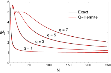
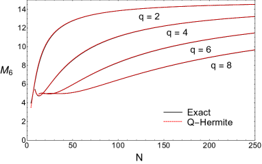
Figure 5: The $N$-dependence of the sixth moment of the eigenvalue density of the SYK model for $q=1,\;3,\;5,\;7$ (left) and $q=2,\;4,\;5,\;8$ (right). We compare the exact result (solid curve) to the Q-Hermite result (dashed).

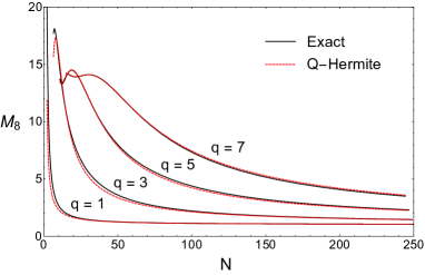
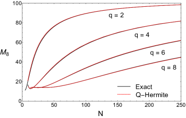
Figure 6: The $N$-dependence of the eighth moment of the eigenvalue density of the SYK model for $q=1,\;3,\;5,\;7$ (left) and $q=2,\;4,\;5,\;8$ (right). We compare the exact result (solid curve) to the Q-Hermite result (dashed).

8 The nature of the Q-Hermite approximation and higher order corrections

The results we have obtained are, at least superficially, contradictory. The $1/N^{2}$ correction to the moments of the Q-Hermite approximation, one of the main result of the paper, does not improve the spectral density in a uniform sense. At the same time the exact computation of low order moments (up to 8th moment), show that the Q-Hermite approximation gives surprisingly accurate results even for relatively small $N$. Adding to this point, the $1/N^{2}$ correction we have obtained in this paper only improves the Q-Hermite for $2p\ll N/q^{2}$. At small $N$, it actually makes the approximation worse than using Q-Hermite results alone even for relatively small $p$.

All the above suggests that the Q-Hermite approximation should be understood as a re-summed finite $N$ result, which happens to be $1/N$-exact in the large $N$ expansion, while the extra $1/N^{2}$ corrections from triangle counting are strictly asymptotic. However, a resummation that is only $1/N$ exact does not imply that the Q-Hermite approximation must be so accurate at finite $N$. To achieve further understanding let us expand the Q-Hermite moments in powers of $1/N$,

$$\frac{M_{2p}^{\text{QH, even $q$}}}{M_{2}^{p}}= (2p-1)!!\left\{1-\frac{2}{3}{p\choose 2}\frac{q^{2}}{N}\right.$$

$$+\left.\left[\frac{1}{45}{p\choose 2}(5p^{2}-p+12)q^{4}-\frac{4}{3}{p\choose 2}q^{3}+\frac{2}{3}{p\choose 2}q^{2}\right]\frac{1}{N^{2}}\right\}+O\left(\frac{1}{N^{3}}\right),$$ (86)

and

$$\frac{M_{2p}^{\text{QH, odd $q$}}}{M_{2}^{p}}=1+2{p\choose 2}\frac{q^{2}}{N}+\left[\frac{p(p-1)^{2}(p-4)}{2}q^{4}+4{p\choose 2}q^{3}-2{p\choose 2}q^{2}\right]\frac{1}{N^{2}}+O\left(\frac{1}{N^{3}}\right),\hskip 14.22636pt$$ (87)

where we have used the expansion of $\eta$ and the identities given in appendix C to perform the sums $\sum_{i}(-1)^{qE_{i}}E_{i}$ and $\sum_{i}(-1)^{qE_{i}}E_{i}^{2}$. Comparing this to the difference

$$\frac{M_{2p}^{\text{even $q$}}-M_{2p}^{\text{QH, even $q$}}}{M_{2}^{p}}=-\frac{8}{15}(2p-1)!!\binom{p}{3}\frac{q^{3}}{N^{2}}+O\left(\frac{1}{N^{3}}\right),$$ (88)

and

$$\frac{M_{2p}^{\text{odd $q$}}-M_{2p}^{\text{QH, odd $q$}}}{M_{2}^{p}}=8\binom{p}{3}\frac{q^{3}}{N^{2}}+O\left(\frac{1}{N^{3}}\right),$$ (89)

we observe that the Q-Hermite approximation is not only exact at order $1/N$, but also almost exact at order $1/N^{2}$ in the following sense:

• The Q-Hermite approximation captures the term $q^{4}/N^{2}$, which is the only term of order $1/N^{2}$ that survives in the scaling limit $N\to\infty$ with $q^{2}/N=\text{constant}$. We have already seen that this property holds to all orders in $q^{2}/N$.

• Even for fixed $q$, the Q-Hermite approximation contains the dominant contribution to moments, that is, the leading coefficients of $1/N^{2}$ in (8) and (87) go as $p^{4}q^{4}$, while the corrections in (88) and (89) go as $p^{3}q^{3}$, and we have $p^{4}q^{4}\gg p^{3}q^{3}$ already for relatively small $p$ and $q$.

The second property is also likely to hold to all orders in $1/N$.

Note that in the truncated form of the Q-Hermite result (8), the corresponding spectral density at each order is a Gaussian or a derivative of Gaussian with the same distribution width, so is the spectral density of the extra correction (88). Therefore the breakdown of the $1/N$ expansion for $x=E/E_{0}\approx 1$ discussed at the end of section 6.1 is really an artefact of the asymptotic nature of this expansion.

9 Conclusions and Outlook

We have obtained analytically an exact expression for the moments of the $q$-body SYK model. For any $q$, we have computed them explicitly up to $1/N^{2}$ order. One surprising result of the calculation of the $1/N^{2}$ order is that it allows a simple and beautiful geometric interpretation in the form of triangular loops of the intersection graphs. The $1/N$ corrections which are part of the Q-Hermite approximation are also geometric in nature and are given by the contribution from the edges. Our results can be generalized to higher orders in $1/N$. Preliminary results for the $1/N^{3}$ correction to the moments indicate they are also characterized by the geometry of the intersection graphs in a simple manner. From a more mathematical perspective, they generate a remarkable set of graph-theoretic identities. In particular, the $1/N^{3}$ computation enumerates a particular linear combination of the last three geometric objects in table 3. It is one of the miracles of the SYK model that the $1/N^{2}$ and even higher order corrections can be calculated analytically. On top of this, given that we have an exact expression for all contraction diagrams contributing to the moments, this might be an indication that the moment problem of the SYK model is completely solvable. In future work we hope to elaborate on this question.

The original motivation to carry out the moments calculation was to obtain a more accurate description of the spectral density and also, closely related, to understand better why the Q-Hermite approximation, which reproduces only the $1/N$ correction to the exact moments of the SYK model, is so close to the numerical SYK spectral density at least for even $q$. Even more remarkable is that the Q-Hermite spectral density exactly reproduces the temperature dependence of the free energy of the SYK model to leading order in $1/q^{2}$ at all temperatures both for even and odd $q$. For the moment, we have at best partial answers to these questions.

We have found that $1/N^{2}$ corrections to the moments, though exact, lead to a correction to the Q-Hermite spectral density which is only accurate sufficiently far away from the tail of the spectrum. As the spectral edge is approached, it gives unphysical results. This is indeed consistent with the fact that, close to the edge of the spectrum, the density is $1/N$ exact Stanford:2017thb ; Bagrets:2017pwq ; Belokurov:2017eit , so in this spectral region, the $1/N^{2}$ correction must be an artefact of the asymptotic expansion in $1/N$. In order to understand the reason for this unphysical behavior we first note that the in large $N$ limit at fixed $q$, $\eta\to(-1)^{q}$ and the Q-Hermite spectral density, the leading term of the expansion, tends to a Gaussian for even $q$ and to $\delta$-functions for odd $q$. Interestingly, the $1/N^{2}$ correction to the spectral density can be expressed in terms of derivatives of this large $N$ limit of the spectral density which strongly suggests that, in terms of a nonlinear $\sigma$-model for the spectral density, the $1/N$ corrections are an expansion about the trivial saddle point. We expect that the spectral edge of the Q-Hermite result is given by a non-trivial saddle point of this effective $\sigma$-model. Indeed a similar effect is observed in the calculation of $1/N$ corrections to the semi-circle law in random matrix theory verbaarschot1984 . It is not clear to us how to re-sum the asymptotic $1/N$ expansion so that it yields a vanishing $1/N^{2}$ correction to the density close to the edge of the spectrum. In fact, we would need an expansion to all orders in $1/N$ to do that. An issue that further complicates the solution of this problem is the non-commutativity of the large $p$ (order of the moment) and the large $N$ limit. The main contribution for moments of order $p\gg N/q^{2}$ comes from the edge of the spectrum, while when we first take the large $N$ limit the main contribution to the moments resides in the bulk of the spectrum. The $1/N^{2}$ corrections also share this nonuniform large $N$ behavior.

Regarding the reason behind the unexpected close agreement between the Q-Hermite density and the exact spectral density of the SYK model, we have found that the leading $1/N^{2}$ contribution in $q$ to the $2p$-th moment, which scales as $p^{4}q^{4}/N^{2}$, is actually included in the Q-Hermite result which helps explain why this approximation, with a difference from the exact result that is also subleading in $p$, goes beyond its natural limit of applicability. However, this does not help explain why the full exact $1/N^{2}$ correction to the density gives worse results than the Q-Hermite approach such as spurious $1/N^{2}$ corrections to the density close to the ground state. In future work we plan to address some of these problems.

Appendix A Calculation of the $1/N^{2}$ corrections

The starting point is the general formula (4) for $\eta_{G}$, which we replicate here for easier access of reading:

$$\begin{split}(-1)^{qE}\eta_{G}&=\binom{N}{q}^{-V}\sum\limits_{\{d_{\alpha_{k}\alpha_{l}}\}}\sum\limits_{\{d_{\alpha_{k}\alpha_{l}\alpha_{m}}\}}\cdots\sum\limits_{\{d_{\alpha_{1}\ldots\alpha_{V}}\}}(-1)^{c(G)}\frac{N!}{(N-Vq+d_{2}+2d_{3}+3d_{4}+\cdots)!}\\ &\times\prod_{k=1}^{V}\frac{1}{(q-d_{\alpha_{k}*}-d_{\alpha_{k}**})!}\prod_{1\leq i<j\leq V}\frac{1}{d_{\alpha_{i}\alpha_{j}}!}\prod_{1\leq i<j<k\leq V}\frac{1}{d_{\alpha_{i}\alpha_{j}\alpha_{k}}!}\cdots\frac{1}{d_{\alpha_{1}\alpha_{2}\cdots\alpha_{V}}!}.\end{split}$$ (90)

We already argued in eq. (42) that the orders in $1/N$ is controlled by the term

$${N\choose q}^{-V}\frac{N!}{(N-Vq+d_{2}+2d_{3}+\cdots)!}\sim N^{-d_{2}-2d_{3}-\cdots}.$$

Note that because of cancellations, the sum (90) may be of higher order in $1/N$, for example if a diagram contains nested contractions. Hence the following four cases contribute to the order of $1/N^{2}$:

• $d_{2}=0,\quad d_{k\geq 3}=0$;

• $d_{2}=1,\quad d_{k\geq 3}=0$;

• $d_{2}=2,\quad d_{k\geq 3}=0$;

• $d_{3}=1,\quad d_{k\neq 3}=0$.

We will compute each of the cases and sum them up. Note the summation indices in (4) are $d_{\alpha_{i_{1}}\cdots\alpha_{i_{k}}}$, which involves all the $k$-vertex structures in an intersection graph $G$. For example, the sum over $d_{\alpha_{i_{1}}\alpha_{i_{2}}}$ involves summing over all edges that connect arbitrary two vertices in $G$, and there are $V(V-1)/2$ such edges. Hence, the edges we need to sum over are more than just the edges of $G$ itself, and to aid the forthcoming computation, we complete the graph $G$ by adding dashed lines between all vertices that are not connected by a solid line. In graph theory this is known as the completion of a graph. In figure 7 we illustrate two examples of such graph completion.

Figure 7: Graph completion for a 3-vertex graph and 4-vertex graph. The resulting graphs have edges between each pair of vertices. This is equivalent to the edge-2 coloring (i.e. that we use two different colors to color a graph) of complete graphs (i.e. graphs where each pair of vertices is connected by an edge).

For a completed graph, we denote by $w_{0},w_{1},w_{2}$ the numbers of wedges with 0, 1 and 2 solid lines, and by $n_{0},n_{1},n_{2},n_{3}$ the numbers of triangles with 0, 1, 2 and 3 solid lines (see table 4), which will be useful for the computations to come.

Table 4: Definition of $w_{0},w_{1},w_{2}$ and $n_{0},n_{1},n_{2},n_{3}$.

A.1 Cases with $d_{k\geq 3}=0$

In this case the general expression for contractions reduces to

$$(-1)^{qE}\eta_{G} = \binom{N}{q}^{-V}\sum\limits_{\{d_{\alpha_{k}\alpha_{l}}\}}(-1)^{c(G)}\frac{N!}{(N-Vq+d_{2})!}$$ (91)

$$\times\prod_{k=1}^{V}\frac{1}{(q-d_{\alpha_{k}*}-d_{\alpha_{k}**}-\cdots)!}\prod_{1\leq i<j\leq V}\frac{1}{d_{\alpha_{i}\alpha_{j}}!},$$

where

$$c(G)=\sum_{k=1}^{E}c_{\alpha_{i_{k}}\alpha_{j_{k}}}=\sum_{k=1}^{E}d_{\alpha_{i_{k}}\alpha_{j_{k}}}.$$ (92)

Note the second equality of (92) holds because we are working with the particular case $d_{k\geq 3}=0$. To order $1/N^{2}$ we have three cases, $d_{2}=0$, $d_{2}=1$ and $d_{2}=2$ which we will analyze next.

Case $d_{2}=0$. The result (91) for a contraction diagram simplifies to

$$(-1)^{qE}\eta_{G}^{d_{2}=0}= \frac{N!(N-q)!^{V}}{(N-Vq)!N!^{V}}$$

$$= 1-\frac{q^{2}}{N}{V\choose 2}+\frac{1}{2}\frac{q^{2}}{N^{2}}{V\choose 2}-\frac{1}{3}\frac{q^{3}}{N^{2}}{V\choose 2}(V+1)+\frac{1}{2}\frac{q^{4}}{N^{2}}{V\choose 2}^{2}+O(1/N^{3}).$$ (93)

Case $d_{2}=1$. In this case, among the $\binom{V}{2}$ possible $d_{\alpha_{k}\alpha_{l}}$ we sum over, $E$ of them occur in the set of edges of $G$ (solid lines in a completed graph) and they give $c(G)=1$, while ${V\choose 2}-E$ of them are not in this set of edges (dashed lines in the completed graph) and they give $c(G)=0$. So this case contributes to $\eta_{G}$ by the following expression:

$$(-1)^{Eq}\eta_{G}^{d_{2}=1}= \frac{N!(N-q)!^{V}}{(N-Vq)!N!^{V}}\frac{q^{2}}{N-Vq+1}\left({V\choose 2}-2E\right)$$

$$= \left[\frac{q^{2}}{N}+\frac{q^{2}}{N^{2}}\left(Vq-1-q^{2}{V\choose 2}\right)\right]\left({V\choose 2}-2E\right)+O(1/N^{3}).$$ (94)

Case $d_{2}=2$. When one of the $d_{\alpha_{k}\alpha_{l}}=2$ then either $c(G)=2$ or $c(G)=0$ and in both cases the phase factor is equal to 1. This results in the contribution

$$(-1)^{Eq}\eta_{G}={V\choose 2}\frac{N!(N-q)!^{V}}{(N-Vq)!N!^{V}}\frac{q^{2}(q-1)^{2}}{2(N-Vq+2)(N-Vq+1)}={V\choose 2}\frac{q^{2}(q-1)^{2}}{2N^{2}}+O(1/N^{3}),$$ (95)

The case with two of the $d_{\alpha_{k}\alpha_{l}}$ equal to 1 is more complicated because we have to distinguish the case where they share a common index and the case where they do not. If they do not share a common index the combinatorial factor apart from the phase factor is

$$\frac{N!(N-q)!^{V}}{(N-Vq)!N!^{V}}\frac{q^{4}}{(N-Vq+2)(N-Vq+1)}=\frac{q^{4}}{N^{2}}+O(1/N^{3}).$$ (96)

while when they share a common index we obtain

$$\frac{N!(N-q)!^{V}}{(N-Vq)!N!^{V}}\frac{q^{3}(q-1)}{(N-Vq+2)(N-Vq+1)}=\frac{q^{3}(q-1)}{N^{2}}+O(1/N^{3}).$$ (97)

The coefficient of the $q^{4}$ term is the same in both cases which simplifies the counting. We have ${E\choose 2}$ pairs of indices with $c(G)=2$, $E({V\choose 2}-E)$ pairs with $c(G)=1$ and ${V(V-1)/2-E\choose 2}$ pairs with $c(G)=0$. Summing over the $\{d_{\alpha_{k}\alpha_{l}}\}$ also including pairs that share a common index, adding the $-q^{3}/N^{2}$ contribution from (97) which was not accounted for in the previous counting, we obtain to order $1/N^{2}$

$$(-1)^{Eq}\eta_{G}^{d_{2}=2}= \left[{E\choose 2}-E\left({V\choose 2}-E\right)+{V(V-1)/2-E\choose 2}\right]\frac{q^{4}}{N^{2}}+(-1)^{Eq}\eta_{G}^{w},$$ (98)

where we have separated the contribution of pairs that share a common index,

$$(-1)^{Eq}\eta_{G}^{w}=-\frac{q^{3}}{N^{2}}(w_{0}-w_{1}+w_{2}),$$ (99)

because it combines naturally with the contributions that will be discussed in the next subsection. The $w_{0},w_{1}$ and $w_{2}$ are defined in table  4, they will give $c(G)=0,1,2$, respectively, and hence the signs in (99).

Summing all the terms with $d_{k\geq 3}=0$, i.e. eqs. (A.1), (A.1) and (98), the result simplifies to

$$(-1)^{Eq}\eta_{G}^{d_{k\geq 3}=0}=1-\frac{2Eq^{2}}{N}+\bigg{\{}2Eq^{2}+\Big{[}-2EV+2{V\choose 3}\Big{]}q^{3}+2E^{2}q^{4}\bigg{\}}\frac{1}{N^{2}}+\frac{q^{3}}{N^{2}}(-w_{0}+w_{1}-w_{2}).$$ (100)

A.2 Cases with $d_{3}=1$

When $d_{3}=1$ to order $1/N^{2}$ only the $d_{2}=0$ terms contribute. The result for a contraction diagram is then given by

$$(-1)^{Eq}\eta_{G}^{d_{3}=1} = \frac{N!(N-q)!^{V}}{(N-Vq)!N!^{V}}\sum\limits_{\{d_{\alpha_{k}\alpha_{l}\alpha_{m}}\}}(-1)^{c(G)}\frac{q^{3}}{(N-Vq+2)(N-Vq+1)}$$

$$= \sum\limits_{\{d_{\alpha_{k}\alpha_{l}\alpha_{m}}\}}(-1)^{c(G)}\frac{q^{3}}{N^{2}}+O(1/N^{3}),$$

where

$$c(G)=\sum_{k=1}^{E}c_{\alpha_{i_{k}}\alpha_{j_{k}}}=\sum_{k=1}^{E}d_{\alpha_{i_{k}}\alpha_{j_{k}}*}.$$ (102)

The second equality (102) is true because we are working in the particular case where $d_{k\neq 3}=0$, and we remind the reader that there is another summation implied by the “$*$” in the subscript. Either 0, 1, 2 or 3 of the edges of $d_{\alpha_{k}\alpha_{l}\alpha_{m}}$ can be part of the edges that occur in $c(G)$, and their total number are $n_{0}$, $n_{1}$, $n_{2}$ or $n_{3}$ respectively, as defined in table 4. We thus obtain the contribution

$$(-1)^{Eq}\eta_{G}^{d_{3}=1} = \frac{q^{3}}{N^{2}}(n_{0}-n_{1}+n_{2}-n_{3}).$$ (103)

Including the contribution of the wedges in eq. (99), the total $q^{3}/N^{2}$ contribution is given by

$$(-1)^{Eq}(\eta_{G}^{d_{3}=1}+\eta_{G}^{w})=\frac{q^{3}}{N^{2}}(-w_{0}+w_{1}-w_{2}+n_{0}-n_{1}+n_{2}-n_{3}).$$ (104)

From the graphical interpretation of these quantities (see Table 4), it is clear that

$$w_{0}=3n_{0}+n_{1},\qquad w_{1}=2n_{1}+2n_{2},\qquad w_{2}=n_{2}+3n_{3}.$$ (105)

The reason is that each wedge is contained in one and only one triangle, and the identities follow by counting in each type of triangle how many wedges of different types occur. This results in the simplification

$$(-1)^{Eq}(\eta_{G}^{d_{3}=1}+\eta_{G}^{w})=\frac{q^{3}}{N^{2}}(-2n_{0}+2n_{2}-4n_{3}).$$ (106)

We have the obvious identities goodman1959

$$n_{1}+2n_{2}+3n_{3} = (V-2)E,$$ (107)

$$n_{0}+n_{1}+n_{2}+n_{3} = {V\choose 3}.$$ (108)

The first identity can be seen as follows. If we have an edge, it can be combined with 0, 1, or 2 other edges to from a triangle with one solid edge, two solid edges, or three solid edges, respectively. In total there are $E(V-2)$ possibilities to combine any edge with the remaining vertices, which gives the right hand side of this identity. The left-hand side counts the same thing triangle by triangle. That is, a triangle with one solid edge occurs once, a triangle with two solid edges is counted twice because each of the solid edges can be taken as the starting point in $E$. For the same reason a solid triangle is counted three times in $(V-2)E$, and hence the identity. By subtracting the two identities we find

$$-n_{0}+n_{2}+2n_{3}=(V-2)E-{V\choose 3}.$$ (109)

The total contribution of the wedge and triangles can thus be written as

$$(-1)^{Eq}(\eta_{G}^{d_{3}=1}+\eta_{G}^{w})=\frac{q^{3}}{N^{2}}\left(-8n_{3}+2(V-2)E-2{V\choose 3}\right).$$ (110)

Adding the thus contribution to the $d_{k\leq 2}$ contributions (see eq. (100)) we obtain

$$(-1)^{Eq}(\eta_{G}^{d_{{k\leq 2}}}+\eta_{G}^{d_{3}=1})=1-\frac{2Eq^{2}}{N}+2E\frac{q^{2}}{N^{2}}-4E\frac{q^{3}}{N^{2}}+2E^{2}\frac{q^{4}}{N^{2}}-8n_{3}\frac{q^{3}}{N^{2}}.$$ (111)

Comparing this to the Q-Hermite result, the $1/N^{2}$ correction simplifies to

$$(-1)^{Eq}(\eta_{G}^{d_{{k\leq 2}}}+\eta_{G}^{d_{3}=1})=(-1)^{Eq}\eta^{E}-8n_{3}\frac{q^{3}}{N^{2}}+O(1/N^{3}).$$ (112)

This proves (29).

Appendix B Scaling limit of $\eta$

To obtain the large $N$ double scaling limit of $\eta$ at fixed $q^{2}/N$ we express $\eta$ in terms of the hypergeometric function as

$$\eta={N\choose q}^{-1}{N-q\choose q}{\,}_{2}F_{1}(-q,-q,N+1-2q,-1).$$ (113)

The double scaling limit of the binomial factor is given by

$${N\choose q}^{-1}{N-q\choose q}\approx\left(1-\frac{q}{N}\right)^{q}\sim e^{-q^{2}/N}.$$ (114)

The hypergeometric function $u:={}_{2}F_{1}(-q,-q,N+1-2q,z)$ satisfies the differential equation

$$z(1-z)\frac{d^{2}u}{dz^{2}}+(N+1-2q+(2q-1)z)\frac{du}{dz}-q^{2}u=0.$$ (115)

In the double scaling limit this simplifies to

$$N\frac{du}{dz}-q^{2}u=0,$$ (116)

which is solved by

$$u=ce^{q^{2}z/N}.$$ (117)

The constant is fixed to $c=1$ by the requirement that $\eta=1$ for $z=1$. For $z=-1$ we thus obtain the asymptotic double scaling limit

$${}_{2}F_{1}(-q,-q,N+1-2q,-1)\sim e^{-q^{2}/N},$$ (118)

and using eq. (114) this results in the scaling limit

$$\eta\sim e^{-2q^{2}/N}.$$ (119)

Appendix C Edge counting from the Riordan-Touchard formula

To evaluate the $1/N$ and $1/N^{2}$ contributions to the Q-Hermite moments we need the sums

$$\sum\limits_{i=1}^{(2p-1)!!}(-1)^{qE_{i}}E_{i}\qquad{\rm and}\qquad\sum\limits_{i=1}^{(2p-1)!!}(-1)^{qE_{i}}{E_{i}}^{2}.$$ (120)

They follow from the first and second derivatives of the Riordan-Touchard formula at $\eta=1$

$$\phi_{p}(\eta):=\sum\limits_{i=1}^{(2p-1)!!}\eta^{E_{i}}=\frac{1}{(1-\eta)^{p}}\sum\limits_{k=-p}^{p}(-1)^{k}\eta^{k(k-1)/2}\binom{2p}{p+k},$$ (121)

where the sum is over all contractions for the $2p$-th moment, and $E_{i}$ is the number of crossing for the $i$-th chord diagram. Below we will show that

$$\phi^{\prime}_{p}(1) =\sum\limits_{i=1}^{(2p-1)!!}{E_{i}}=\frac{1}{3}\binom{p}{2}(2p-1)!!,$$ (122)

$$\phi^{\prime\prime}_{p}(1) =\sum\limits_{i=1}^{(2p-1)!!}{E_{i}}({E_{i}}-1)=\frac{1}{90}\binom{p}{2}(5p^{2}-p-18)(2p-1)!!,$$ (123)

$$-\phi^{\prime}_{p}(-1) =\sum\limits_{i=1}^{(2p-1)!!}(-1)^{{E_{i}}}{E_{i}}=-\binom{p}{2},$$ (124)

$$\phi^{\prime\prime}_{p}(-1) =\sum\limits_{i=1}^{(2p-1)!!}(-1)^{{E_{i}}}{E_{i}}({E_{i}}-1)=6{p\choose 4}.$$ (125)

The first two equalities were already shown in flajolet2000 . Here, we give the key ingredients of the proof. We start from the following integral representation of $\phi_{p}$,

$$\phi_{p}(e^{t})=\frac{1}{\sqrt{2\pi}}\int_{-\infty}^{\infty}e^{-x^{2}/2}x^{2p}H(x,t)^{p}dx,$$ (126)

where

$$H(x,t)=\frac{2\sinh^{2}(x\sqrt{t}/2-t/4)}{x^{2}\exp(t/2)\sinh(t/2)}.$$ (127)

This can be used to show that $\phi_{p}(1)=(2p-1)!!$. It also follows

$$\phi_{p}(-1)=\frac{1}{\sqrt{2\pi}}\int_{-\infty}^{\infty}e^{-x^{2}/2}(i\sinh(x\sqrt{\pi i}+1)^{p}dx=1.$$ (128)

To obtain the derivatives of $\phi_{p}(\eta)$ we expand $H(x,t)^{p}$ about $t=0$,

$$H(x,t)^{p}=1-\frac{p\sqrt{t}}{x}+\frac{p(-3+6p-6x^{2}+x^{4})t}{12x^{2}}+O(t^{3/2}).$$ (129)

Then

$$\begin{split}\lim_{\eta\to 1}\phi^{\prime}_{p}(\eta)&=\lim_{t\to 0}e^{-t}\frac{d\phi(e^{t})}{dt}\\ &=\frac{1}{\sqrt{2\pi}}\int_{-\infty}^{\infty}e^{-x^{2}/2}x^{2p}\frac{p(-3+6p-6x^{2}+x^{4})}{12x^{2}}dx\\ \ &=\frac{1}{3}\binom{p}{2}(2p-1)!!.\end{split}$$ (130)

This proves the first equality (122). The second equality (123) can be similarly proved.

The proof of the last two equalities (124) and (125) requires some more work. Using the integral representation (126) of $\phi_{p}(\eta)$ we obtain

$$\phi^{\prime}_{p}(-1)= \left[e^{-t}\frac{d\phi_{p}(e^{t})}{dt}\right]_{t=i\pi}$$

$$= -\frac{1}{\sqrt{2\pi}}\int_{-\infty}^{\infty}e^{-x^{2}/2}\left\{p\left[i\sinh(\sqrt{\pi i}x)+1\right]^{p-1}\left(i\cosh(\sqrt{\pi i}x)\right)\left(\frac{x}{2\sqrt{\pi i}}-\frac{1}{2}\right)\right.$$

$$\qquad\qquad\qquad\qquad\quad\left.-\frac{p}{2}\left[i\sinh(\sqrt{\pi i}x)+1\right]^{p}\right\}dx$$

$$= -\frac{p}{\sqrt{\pi}}\int_{-\infty}^{\infty}e^{-y^{2}}\left\{\left[i\sinh(\sqrt{2\pi i}y)+1\right]^{p-1}\left(i\cosh(\sqrt{2\pi i}y)\right)\left(\frac{y}{\sqrt{2\pi i}}-\frac{1}{2}\right)\right.$$

$$\qquad\qquad\qquad\qquad\left.-\frac{1}{2}\left[i\sinh(\sqrt{2\pi i}y)+1\right]^{p}\right\}dy,$$ (131)

where we have substituted $x=\sqrt{2}y$ for the last equality. It is straightforward to show

$$I_{1,p}:=\frac{1}{\sqrt{\pi}}\int_{-\infty}^{\infty}dye^{-y^{2}}\left[i\sinh(\sqrt{2\pi i}y)+1\right]^{p}=1,$$ (132)

$$I_{2,p}:=\frac{1}{\sqrt{\pi}}\int_{-\infty}^{\infty}dye^{-y^{2}}\left[i\sinh(\sqrt{2\pi i}y)+1\right]^{p}\left(i\cosh(\sqrt{2\pi i}y)\right)=-1,$$ (133)

$$I_{3,p}:=\frac{1}{\sqrt{\pi}}\int_{-\infty}^{\infty}dye^{-y^{2}}y\left[i\sinh(\sqrt{2\pi i}y)+1\right]^{p}\left(i\cosh(\sqrt{2\pi i}y)\right)=-\frac{\sqrt{2\pi i}}{2}p.$$ (134)

Hence,

$$\phi^{\prime}_{p}(-1)=-p\left(\frac{1}{\sqrt{2\pi i}}I_{3,p-1}-\frac{1}{2}I_{2,p-1}-\frac{1}{2}I_{1,p}\right)=\binom{p}{2},$$ (135)

which proves (124).

To prove the last equality, we start with

$$\begin{split}\phi_{p}^{\prime\prime}(-1)=&\left[e^{-t}\frac{d}{dt}\left(e^{-t}\frac{d\phi_{p}(e^{t})}{dt}\right)\right]_{t=i\pi}=\phi_{p}^{\prime}(-1)+\left[\frac{d^{2}\phi_{p}(e^{t})}{dt^{2}}\right]_{t=i\pi}=\binom{p}{2}+\left.\frac{d^{2}\phi_{p}(e^{t})}{dt^{2}}\right|_{t=i\pi}.\end{split}$$ (136)

The second derivative can be expressed in terms of the integral representation (126) of $\phi_{p}(\eta)$ as

$$\begin{split}\left.\frac{d^{2}\phi_{p}(e^{t})}{dt^{2}}\right|_{t=i\pi}=&\frac{1}{\sqrt{2\pi}}\int_{-\infty}^{\infty}dx\ e^{-x^{2}/2}x^{2p}\left(\partial^{2}_{t}[H(x,t)^{p}]\right)_{t=i\pi}\\ =&\frac{1}{\sqrt{\pi}}\int_{-\infty}^{\infty}dy\ e^{-y^{2}}(\sqrt{2}y)^{2p}\left(\partial^{2}_{t}[H(\sqrt{2}y,t)^{p}]\right)_{t=i\pi}.\end{split}$$ (137)

After some tedious but straightforward manipulations, we get

$$\begin{split}\left.\frac{d^{2}\phi_{p}(e^{t})}{dt^{2}}\right|_{t=i\pi}=&\left(\frac{p}{4}-\frac{p^{2}}{2}\right)I_{1,p-1}+\frac{p^{2}}{2}I_{2,p-1}-\left(\frac{p}{4}-\frac{p^{2}}{2}\right)I_{1,p}\\ &+e^{i3\pi/4}\left(\frac{p}{\sqrt{2\pi}}-\sqrt{\frac{2}{\pi}}p^{2}\right)I_{4,p-1}+i\left(\frac{e^{i\pi/4}}{\sqrt{2\pi}}p^{2}-\frac{e^{i3\pi/4}}{2\sqrt{2}\pi^{3/2}}p\right)I_{3,p-1}\\ &+\frac{e^{i3\pi/4}}{\sqrt{2\pi}}p^{2}I_{4,p}+\frac{i}{2\pi}(2p^{2}-p)I_{5,p-1}-\frac{ip^{2}}{2\pi}I_{5,p}\\ =&\frac{1}{4}p(p-4)(p-1)^{2},\end{split}$$ (138)

where we have used two additional integrals to obtain the last line.

$$I_{4,p}:=\frac{1}{\sqrt{\pi}}\int_{-\infty}^{\infty}dye^{-y^{2}}y\left[i\sinh(\sqrt{2\pi i}y)+1\right]^{p}=-\frac{\sqrt{2\pi i}}{2}p,$$ (139)

$$I_{5,p}:=\frac{1}{\sqrt{\pi}}\int_{-\infty}^{\infty}dye^{-y^{2}}y^{2}\left[i\sinh(\sqrt{2\pi i}y)+1\right]^{p}=\frac{1}{2}-\binom{p}{2}\pi i.$$ (140)

This proves (125).

Appendix D Cut-vertices and factorization

Since the subscript space of $\binom{N}{q}$ elements is isotropic we can always fix one index and the result of a diagram does not depend on this index. So summing over this index gives a factor ${N\choose q}$.

We define a cut-vertex as a vertex that when it is cut, the graph becomes disconnected. A graph without any cut-vertex is called a non-separable or a two-connected graph. If we apply the reasoning of the first paragraph to a cut vertex, we immediately arrive at the theorem

Theorem 1.

If a graph $G$ contains a cut-vertex, which separates $G$ into subgraphs $G_{1}$ and $G_{2}$, then

$$\eta_{G}=\eta_{G_{1}}\eta_{G_{2}}.$$

As an example, the following graphs all contain one cut-vertex (drawn in red):

Theorem 1, for example implies,

Appendix E Moments for $q=2$

In this appendix we calculate the moments $M_{2p}/M_{2}^{p}$ to order $1/N^{2}$ for the $q=2$ SYK model.

Since we are interested in large $N$ asymptotics, it is immaterial whether $N$ is even or odd, and for technical simplicity we choose $N$ to be even. The Hamiltonian for $q=2$ model is given by

$$H=i\sum_{i<j}J_{ij}\gamma_{i}\gamma_{j}.$$ (141)

This can be rewritten as cotler2016

$$H=\sum_{k=1}^{N/2}x_{k}(2c_{k}^{\dagger}c_{k}-1),$$ (142)

where $x_{k}$ are the positive eigenvalues of the antisymmetric matrices $J_{ij}$, and $c_{k},c_{k}^{\dagger}$ are the annihilation and creation operators for Dirac fermions. We have

$$\langle\textrm{Tr}(H^{2p})\rangle=\left\langle\sum_{\{s_{k}=\pm 1\}}\left(\sum_{k=1}^{N/2}s_{k}x_{k}\right)^{2p}\right\rangle,$$ (143)

where

$$\sum_{\{s_{k}=\pm 1\}}=\sum_{s_{1}=\pm 1}\sum_{s_{2}=\pm 1}\cdots\sum_{s_{N/2}=\pm 1}.$$ (144)

Thus we can compute the ensemble average by averaging over the joint probability distribution of anti-symmetric Hermitian random matrices mehta2004 ; gross2017 ,

$$P(x_{1},\ldots,x_{N/2})\prod_{l=1}^{N/2}dx_{l}=ce^{-\sum_{k}x_{k}^{2}}\prod_{i<j}(x_{i}^{2}-x_{j}^{2})^{2}\prod_{l=1}^{N/2}dx_{l}.$$ (145)

Here $c$ is a normalization constant, which we have chosen such that $P(x_{1},\ldots,x_{N/2})$ is normalized to unity. Note that the joint probability distribution has the parity symmetry $x_{k}\to-x_{k}$ for each individual variable, so we can we can restrict ourselves to the configuration with only positive $s_{k}$ by compensating with an overall factor $2^{N/2}$. This results in

$$\langle\textrm{Tr}(H^{2p})\rangle=2^{N/2}\left\langle\left(\sum_{k=1}^{N/2}x_{k}\right)^{2p}\right\rangle.$$ (146)

In particular

$$\langle\textrm{Tr}(H^{2})\rangle=2^{N/2}\left\langle\left(\sum_{k=1}^{N/2}x_{k}\right)^{2}\right\rangle=2^{N/2}\frac{N}{2}\langle x_{1}^{2}\rangle,$$ (147)

where we have used $\langle x_{k}\rangle=0$ and $\langle x_{1}^{2}\rangle=\langle x_{2}^{2}\rangle=\ldots=\langle x_{N/2}^{2}\rangle$ because of the parity symmetry and permutation symmetry of $P(x_{1},\ldots,x_{N/2})$. Hence,

$$\frac{M_{2p}}{M_{2}^{p}}=\left.\left\langle\left(\sum_{k=1}^{N/2}x_{k}\right)^{2p}\right\rangle\middle/\left(\frac{N}{2}\langle x_{1}^{2}\rangle\right)^{p}\right..$$ (148)

To isolate the leading orders in $1/N$ we now need to analyze the terms in

$$\left\langle\left(\sum_{k=1}^{N/2}x_{k}\right)^{2p}\right\rangle=\sum_{m_{1}+\cdots+m_{N/2}=p}\frac{(2p)!}{(2m_{1})!(2m_{2})!\cdots(2m_{N/2})!}\left\langle x_{1}^{2m_{1}}x_{2}^{2m_{2}}\cdots x_{N/2}^{2m_{N/2}}\right\rangle$$ (149)

that are leading orders in $N$. Again, because of the permutation symmetry of $P(x_{1},\ldots,x_{N/2})$, the expectation values on the right-hand side of equation (149) only depend on the partition of $p$ into $\{m_{1},m_{2},\cdots,m_{N/2}\}$. Therefore, given a partition with $k$ nonzero $m_{i}$’s, $\{m_{i_{1}},m_{i_{2}},\cdots,m_{i_{k}}\}$ ($i_{1}<i_{2}<\cdots<i_{k}$ by convention), all the expectation values of the form

$$\left\langle x_{j_{1}}^{2m_{i_{1}}}x_{j_{2}}^{2m_{i_{2}}}\cdots x_{j_{k}}^{2m_{i_{k}}}\right\rangle$$ (150)

have the same value and this results in a multiplicity factor $\binom{N/2}{k}$ from choosing $k$-element subsets of $\{x_{1},\ldots,x_{N/2}\}$. It is not too hard to convince oneself that

$$\left.\left\langle x_{j_{1}}^{2m_{i_{1}}}x_{j_{2}}^{2m_{i_{2}}}\cdots x_{j_{k}}^{2m_{i_{k}}}\right\rangle\middle/\langle x_{1}^{2}\rangle^{p}\right.\sim O(1),$$ (151)

so we can isolate the leading terms in $1/N$ from the binomial factors $\binom{N/2}{k}$, and there can be more multiplicity factors from permuting the $x_{j}$’s in the same partition, but that does not bring any factors of $N$. Now it becomes obvious that the leading terms which are relevant to $1/N^{2}$ accuracy are associated with the largest multiplicity factors $\binom{N/2}{p}$, $\binom{N/2}{p-1}$ and $\binom{N/2}{p-2}$. From equation (149), these are the terms

$$M_{2p} = \binom{N/2}{p}\frac{(2p)!}{2^{p}}\left\langle x_{1}^{2}x_{2}^{2}\cdots x_{p}^{2}\right\rangle+\binom{N/2}{p-1}\binom{p-1}{1}\frac{(2p)!}{2^{p-2}4!}\left\langle x_{1}^{4}x_{2}^{2}\cdots x_{p-1}^{2}\right\rangle$$

$$+\binom{N/2}{p-2}\left[\binom{p-2}{2}\frac{(2p)!}{2^{p-4}4!4!}\left\langle x_{1}^{4}x_{2}^{4}x_{3}^{2}\cdots x_{p-2}^{2}\right\rangle+\binom{p-2}{1}\frac{(2p)!}{2^{p-3}6!}\left\langle x_{1}^{6}x_{2}^{2}\cdots x_{p-2}^{2}\right\rangle\right],$$

where the factors $\binom{p-1}{1}$,$\binom{p-2}{2}$ and $\binom{p-2}{1}$ come from permutations within a partition. The rescaled moments are given by

$$\begin{split}\frac{M_{2p}}{M_{2}^{p}}=&\left(\frac{N}{2}\right)^{-p}\binom{N/2}{p}\frac{(2p)!}{2^{p}}\frac{W_{1}}{W_{0}^{p}}+\left(\frac{N}{2}\right)^{-p}\binom{N/2}{p-1}\binom{p-1}{1}\frac{(2p)!}{2^{p-2}4!}\frac{W_{2}}{W_{0}^{p}}\\ &+\left(\frac{N}{2}\right)^{-p}\binom{N/2}{p-2}\left[\binom{p-2}{2}\frac{(2p)!}{2^{p-4}4!4!}\frac{W_{3}}{W_{0}^{p}}+\binom{p-2}{1}\frac{(2p)!}{2^{p-3}6!}\frac{W_{4}}{W_{0}^{p}}\right].\end{split}$$ (153)

where the combinations $W_{k}$ are defined by

$$\begin{split}&W_{0}:=\langle x_{1}^{2}\rangle,\\ &W_{1}:=\left\langle x_{1}^{2}x_{2}^{2}\cdots x_{p}^{2}\right\rangle,\\ &W_{2}:=\left\langle x_{1}^{4}x_{2}^{2}\cdots x_{p-1}^{2}\right\rangle,\\ &W_{3}:=\left\langle x_{1}^{4}x_{2}^{4}x_{3}^{2}\cdots x_{p-2}^{2}\right\rangle,\\ &W_{4}:=\left\langle x_{1}^{6}x_{2}^{2}\cdots x_{p-2}^{2}\right\rangle.\\ \end{split}$$ (154)

Before evaluating these averages we can already expand the prefactors to order $1/N^{2}$,

$$\begin{split}\frac{M_{2p}}{M_{2}^{p}}=&(2p-1)!!\left\{\left[1-2\binom{p}{2}\frac{1}{N}+(3p-1)\binom{p}{3}\frac{1}{N^{2}}\right]\frac{W_{1}}{W_{0}^{p}}\right.\\ &\left.+\frac{1}{3}\binom{p}{2}\left[\frac{2}{N}-4\binom{p-1}{2}\frac{1}{N^{2}}\right]\frac{W_{2}}{W_{0}^{p}}+\frac{4}{N^{2}}\left[\frac{1}{3}\binom{p}{4}\frac{W_{3}}{W_{0}^{p}}+\frac{1}{15}\binom{p}{3}\frac{W_{4}}{W_{0}^{p}}\right]\right\}+O\left(1/N^{3}\right).\end{split}$$ (155)

The averages in (154) are Selberg-type integrals and they can be evaluated by using the recursive relations developed in verbaarschot:1994gr . After some algebra we obtain

$$\begin{split}&W_{0}=\frac{N-1}{2},\\ &W_{1}=\prod_{k=0}^{p-1}\left(\frac{N}{2}-p+k+\frac{1}{2}\right),\\ &W_{2}=\left(N-p+\frac{3}{2}\right)\prod_{k=0}^{p-2}\left(\frac{N}{2}-p+k+\frac{3}{2}\right),\\ &W_{3}=\left(N-p+\frac{3}{2}\right)\left(N-p+\frac{5}{2}\right)\prod_{k=0}^{p-3}\left(\frac{N}{2}-p+k+\frac{5}{2}\right),\\ &W_{4}=\left(N+\frac{1}{2}\right)\left(N-p+\frac{5}{2}\right)\prod_{k=0}^{p-3}\left(\frac{N}{2}-p+k+\frac{5}{2}\right)+\left(\frac{N}{2}-p+2\right)\prod_{k=0}^{p-2}\left(\frac{N}{2}-p+k+\frac{3}{2}\right).\\ \end{split}$$ (156)

Hence, to the relevant orders, we have

$$\begin{split}&\frac{W_{1}}{W_{0}^{p}}=1-2\binom{p}{2}\frac{1}{N}+\frac{1}{3}\binom{p}{2}(3p^{2}-7p-4)\frac{1}{N^{2}}+O\left(\frac{1}{N^{3}}\right),\\ &\frac{W_{2}}{W_{0}^{p}}=2-(2p^{2}-4p-1)\frac{1}{N}+O\left(\frac{1}{N^{2}}\right),\\ &\frac{W_{3}}{W_{0}^{p}}=4+O\left(\frac{1}{N}\right),\\ &\frac{W_{4}}{W_{0}^{p}}=5+O\left(\frac{1}{N}\right).\\ \end{split}$$ (157)

Note that the each leading term is just the number of nested contractions when re-expressing the $W_{k}$ in products of $\textrm{Tr}J^{2k}$ to leading order in $1/N$. Substituting the above results into (155), we finally arrive at

$$\frac{M_{2p}}{M_{2}^{p}}=(2p-1)!!\left[1-\frac{8}{3}\binom{p}{2}\frac{1}{N}+\frac{8}{9}\binom{p}{2}(2p^{2}-2p-1)\frac{1}{N^{2}}\right]+O\left(\frac{1}{N^{3}}\right).$$ (158)

Appendix F Calculation of the eighth moment

The sixth moment was already discussed in garcia2016 and in this appendix we only quote the final result. For the eighth moment we work out all contributions explicitly. Although originally the combinatorics for the eighth moment were obtained by inspection, in several cases we also show how they can be obtained from the general formula (4).

According to the Riordan-Touchard formula we have

$$\sum_{i=1}^{(2p-1)!!}\eta^{E_{i}}=\frac{1}{(1-\eta)^{p}}\sum_{k=-p}^{p}(-1)^{k}\eta^{k(k-1)/2}{2p\choose p+k}.$$ (159)

For $p=3$ the right hand side is given by

$$\sum_{i=1}^{15}\eta^{E_{i}}=5+6\eta+3\eta^{2}+\eta^{3}.$$ (160)

Only the $\eta^{3}$ term deviates from the exact result which is given by

$$\frac{M_{6}}{M_{2}^{3}}=5+6\eta+3\eta^{2}+T_{6},$$ (161)

where

$$T_{6} = {N\choose q}^{-2}\sum_{q_{1}=0}^{q}\sum_{l=0}^{q}\sum_{m=0}^{l}(-1)^{q-q_{1}-m}{N-2q+q_{1}\choose q-l}{2q-2q_{1}\choose m}{N-q\choose q-q_{1}}{q\choose q_{1}}{q_{1}\choose l-m}$$ (162)

$$= {N\choose q}^{-2}\sum_{q_{1}=0}^{q}\sum_{m=0}^{q}(-1)^{q-q_{1}-m}{N-2q+2q_{1}\choose q-m}{2q-2q_{1}\choose m}{N-q\choose q-q_{1}}{q\choose q_{1}}$$

and

$$\eta={N\choose q}^{-1}\sum_{r=0}^{q}(-1)^{q-r}{q\choose r}{N-q\choose q-r}.$$ (163)

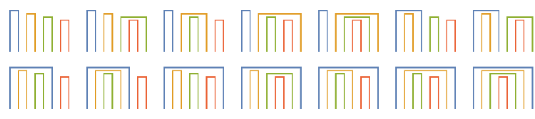
Figure 8: The nested diagrams contributing to the 8th moment.

For $p=4$ the Riordan-Touchard formula yields

$$14+28\eta+28\eta^{2}+20\eta^{3}+10\eta^{4}+4\eta^{5}+\eta^{6},$$ (164)

where the coefficient of $\eta^{E}$ gives the number of diagrams with $E$ crossings. For one and two intersections the crossings can be commuted independently resulting in

$$\frac{M_{8}^{E=0}}{M_{2}^{4}} = 14,$$

$$\frac{M_{8}^{E=1}}{M_{2}^{4}} = 28\eta,$$ (165)

$$\frac{M_{8}^{E=2}}{M_{2}^{4}} = 28\eta^{2},$$

The diagrams corresponding to the contributions (165) are shown in figures 8 to 10.

For $E=3$ we have two different contributions. The first class of twelve diagrams is shown in figure 11, where we can move the $\Gamma_{\alpha}$ to three consecutive pairs with equal indices by three independent pair exchanges. The results of each of these diagrams is given by $\eta^{3}$. The second class of eight diagrams with three intersections contains a structure we first saw in the calculation of the sixth moment (see figure 12). It is given by $T_{6}$ garcia2016 , see eq. (162) and we thus obtain

$$\frac{M_{8}^{E=3}}{M_{2}^{4}} = 12\eta^{3}+8T_{6}.$$ (166)

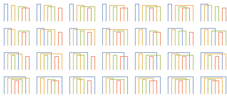
Figure 9: The diagrams with one intersection contributing to the eighth moment.

Figure 10: The diagrams with two intersections contributing to the eighth moment.

Figure 11: Diagrams with three intersections contributing to the eighth moment as $\eta^{3}$.

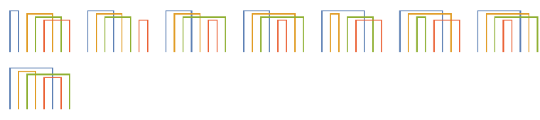
Figure 12: Diagrams with three intersections contributing to the eighth moment as $T_{6}$.

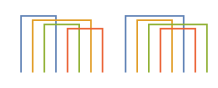
Figure 13: Diagrams with four intersections contributing to the eighth moment as $T_{44}$.

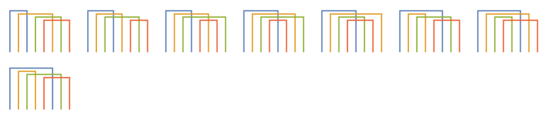
Figure 14: Diagrams with four intersections contributing to the eighth moment as $\eta T_{6}$.

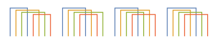
Figure 15: The diagrams with five intersections contributing to the eighth moment as $T_{66}$ which is a new type of contribution.

Figure 16: The only diagram with six intersections contributing to the eighth moment. This diagram has not been encountered before and the result will be denoted by $T_{8}$.

For $E=4$ also two different classes of diagrams contribution to the eighth moment. The two diagrams of the first class are shown in figure 13. The result depends on how many gamma matrices the second and third contraction have in common. It is given by

$$T_{44} = {N\choose q}^{-3}\sum_{q_{1}=0}^{q}\sum_{l_{1}=0}^{q}\sum_{m_{1}=0}^{l_{1}}\sum_{l_{2}=0}^{q}\sum_{m_{2}=0}^{l_{1}}(-1)^{m_{1}+m_{2}}{N-q\choose q-q_{1}}{q\choose q_{1}}{N-2q+q_{1}\choose q-l_{1}}$$ (167)

$$\times{2q-2q_{1}\choose m_{1}}{q_{1}\choose l_{1}-m_{1}}{N-2q+q_{1}\choose q-l_{2}}{q_{1}\choose l_{2}-m_{2}}{2q-2q_{1}\choose m_{2}}.$$

$$= {N\choose q}^{-3}\sum_{q_{1}=0}^{q}\sum_{m_{1}=0}^{q}\sum_{m_{2}=0}^{q}(-1)^{m_{1}+m_{2}}{N-q\choose q-q_{1}}{q\choose q_{1}}{N-2q+2q_{1}\choose q-m_{1}}$$

$$\times{2q-2q_{1}\choose m_{1}}{N-2q+2q_{1}\choose q-m_{2}}{2q-2q_{1}\choose m_{2}}.$$

The second class of eight diagrams has one intersecting contraction which can be removed by a pair exchange, and three other contractions which have three intersections and contribute as $T_{6}$ (see figure 14). The total contribution of diagrams with four intersections is thus given by

$$\frac{M_{8}^{E=4}}{M_{2}^{4}} = 2T_{44}+8\eta T_{6}.$$ (168)

There are four diagrams with 5 intersections which are shown in figure 15. The contribution of these diagrams cannot be decomposed into contributions we have seen before. The result of each diagram is given by

$$T_{66} = {N\choose q}^{-3}\sum_{q_{1}=0}^{q}\sum_{l_{1}=0}^{q}\sum_{m_{1}=0}^{l_{1}}\sum_{l_{2}=0}^{q}\sum_{m_{2}=0}^{l_{2}}(-1)^{q+q_{1}+m_{1}+m_{2}}{N-q\choose q-q_{1}}{q\choose q_{1}}{N-2q+q_{1}\choose q-l_{1}}$$ (169)

$$\times{2q-2q_{1}\choose m_{1}}{q_{1}\choose l_{1}-m_{1}}{N-2q+q_{1}\choose q-l_{2}}{2q-2q_{1}\choose m_{2}}{q_{1}\choose l_{2}-m_{2}}$$

$$= {N\choose q}^{-3}\sum_{q_{1}=0}^{q}\sum_{m_{1}=0}^{q}\sum_{m_{2}=0}^{q}(-1)^{q+q_{1}+m_{1}+m_{2}}{N-q\choose q-q_{1}}{q\choose q_{1}}{N-2q+2q_{1}\choose q-m_{1}}$$

$$\times{2q-2q_{1}\choose m_{1}}{N-2q+2q_{1}\choose q-m_{2}}{2q-2q_{1}\choose m_{2}}.$$

The contribution of diagrams with five intersections to the eighth moment is thus given by

$$\frac{M_{8}^{k=5}}{M_{2}^{4}} = 4T_{66}.$$ (170)

The most complicated diagram has six intersections, see figure 16. The result is given by

$$T_{8} = {N\choose q}^{-3}\sum_{q_{1}=0}^{q}\sum_{q_{2}=0}^{q}\sum_{m=0}^{q_{1}}\sum_{n=0}^{2q-2q_{1}}\sum_{k=0}^{m}\sum_{l=0}^{n}\sum_{s=0}^{k}\sum_{t=0}^{l}(-1)^{q_{1}+q_{2}+n+t}{N-q\choose q-q_{1}}{q\choose q_{1}}{2q-2q_{1}\choose n}{q_{1}\choose m}$$ (171)

$$\times{m\choose k}{n\choose l}{N-2q+q_{1}\choose q-k-l}{k\choose s}{l\choose t}{q-k-l\choose q_{2}-s-t}{N-3q+q_{1}+k+l\choose q-q_{2}-(m-k+n-l)}.$$

Using the convolution property of binomial factors, this can be simplified to

$$T_{8} = {N\choose q}^{-3}\sum_{q_{1}=0}^{q}\sum_{q_{2}=0}^{q}\sum_{n=0}^{2q-2q_{1}}\sum_{t=0}^{n}(-1)^{q_{1}+q_{2}+n+t}{N-q\choose q-q_{1}}{q\choose q_{1}}{2q-2q_{1}\choose n}{n\choose t}$$ (172)

$$\times{N-2q+2q_{1}\choose 2q-q_{2}-n}{2q-q_{2}-n\choose q_{2}-t}{2q-2q_{2}\choose q-q_{2}}.$$

The contribution to the fourth moment with six crossings is thus given by

$$\frac{M_{8}^{E=6}}{M_{2}^{4}} = T_{8}.$$ (173)

We have checked the above results in several ways. First, when the phase factor is eliminated the contribution of each diagram evaluates to one. Second, the moments agree with numerical result of the moments obtained from the eigenvalues of the SYK Hamiltonian at finite $N$. Third, for $q=1$ the results agree with the exact analytical result in eq. (51).

In the next subsection we derive the result for $T_{6}$ and $T_{8}$ from the general formula (4).

F.1 Calculation of contributions to the moments starting from the general formula

F.1.1 Calculation of $T_{6}$

The result of the diagram (c) of figure 1 using the general formula (4) is given by

$$T_{6} = {N\choose q}^{-3}\sum_{a,b,c,p}\frac{(-1)^{a+b+c}N!}{(N-3q+a+b+c+2p)!}$$ (174)

$$\times\frac{1}{(q-a-b-p)!(q-a-c-p)!(q-b-c-p)!a!b!c!p!}$$

$$= {N\choose q}^{-3}\sum_{a,b,c,p}(-1)^{a+b+c}{q-a-p\choose b}{q-a-p\choose c}$$

$$\times\frac{N!}{(N-3q+a+b+c+2p)!(q-b-c-p)!a!p!(q-a-p)!(q-a-p)!}.$$

Using $m=b+c$ as new summation variable after summing the first two binomials and absorbing $p$ in $a$ this can be rewritten as

$$T_{6} = {N\choose q}^{-3}\sum_{a,m,p}{2q-2a\choose m}\frac{(-1)^{a+m}N!}{(N-3q+a+m+p)!(q-m-p)!(a-p)!p!(q-a)!(q-a)!}$$ (175)

$$= {N\choose q}^{-3}\sum_{a,m,p}{2q-2a\choose m}{N-2q+a\choose q-m-p}{a\choose p}\frac{(-1)^{a+m}N!}{(N-2q+a)!a!(q-a)!(q-a)!}.\hskip 14.22636pt$$

After performing the sum over $p$ we finally obtain

$$T_{6} = {N\choose q}^{-2}\sum_{a,m}(-1)^{a+m}{2q-2a\choose m}{N-2q+2a\choose q-m}{N-q\choose q-a}{q\choose a},$$ (176)

which is the result obtained in section 7.

F.1.2 Calculation of $T_{8}$

In this subsection we derive the result for the diagram $T_{8}$ starting from the general result (4). We first change from the $d$ representation to the $c$ representation,

$$d_{ab} = c_{ab}-c_{abc}-c_{abd}+c_{abcd},\qquad d_{ac}=c_{ac}-c_{abc}-c_{acd}+c_{abcd},$$

$$d_{ad} = c_{ad}-c_{abd}-c_{acd}+c_{abcd},\qquad d_{bd}=c_{bd}-c_{bcd}-c_{abd}+c_{abcd},$$

$$d_{bc} = c_{bc}-c_{abc}-c_{bcd}+c_{abcd},\qquad d_{cd}=c_{cd}-c_{bcd}-c_{acd}+c_{abcd},$$

$$d_{abc} = c_{abc}-c_{abcd},\qquad d_{abd}=c_{abd}-c_{abcd},$$

$$d_{bcd} = c_{bcd}-c_{abcd},\qquad d_{acd}=c_{acd}-c_{abcd},$$

$$d_{abcd} = c_{abcd}.$$ (177)

Then it can be expressed in terms of binomials as

$$T_{8} ={N\choose q}^{-3}\sum(-1)^{c_{ab}+c_{ac}+c_{ad}+c_{bc}+c_{bd}+c_{cd}}{N-q\choose q-c_{ab}}{q\choose c_{ab}}$$ (178)

$$\times{c_{ab}\choose c_{abc}+c_{abd}-c_{abcd}}{c_{abc}+c_{abd}-c_{abcd}\choose c_{abc}}{c_{abc}\choose c_{abcd}}{c_{ac}-c_{abc}\choose c_{acd}-c_{abcd}}{c_{bc}-c_{abc}\choose c_{bcd}-c_{abcd}}$$

$$\times{q-c_{ab}\choose c_{ac}+c_{ad}-c_{abc}-c_{abd}-c_{acd}+c_{abcd}}{c_{ac}+c_{ad}-c_{abc}-c_{abd}-c_{acd}+c_{abcd}\choose c_{ac}-c_{abc}}$$

$$\times{q-c_{ab}\choose c_{bc}+c_{bd}-c_{abc}-c_{abd}-c_{bcd}+c_{abcd}}{c_{bc}+c_{bd}-c_{abc}-c_{abd}-c_{bcd}+c_{abcd}\choose c_{bc}-c_{abc}}$$

$$\times{N-3q+c_{ab}+c_{bc}+c_{ac}-c_{abc}\choose q-c_{ad}-c_{bd}-c_{cd}+c_{abd}+c_{acd}+c_{bcd}-c_{abcd}}$$

$$\times{N-2q+c_{ab}\choose q-c_{ac}-c_{bc}+c_{abc}}{q-c_{ac}-c_{bc}+c_{abc}\choose c_{cd}-c_{acd}-c_{bcd}+c_{abcd}},$$

where the sum is over the $c_{a_{1}\cdots a_{k}}$. Next, we change the summation variables according to

$$m_{1} = c_{abc}+c_{abd}-c_{abcd},\qquad$$ (179)

$$m_{2a} = c_{ac}+c_{ad}-c_{abc}-c_{abd}-c_{acd}+c_{abcd},\qquad m_{2b}=c_{bc}+c_{bd}-c_{abc}-c_{abd}-c_{bcd}+c_{abcd},$$

$$s_{2a} = c_{acd}-c_{abcd},\qquad s_{2b}=c_{bcd}-c_{abcd},\qquad k_{2a}=c_{ac}-c_{abc},\qquad k_{2b}=c_{bc}-c_{abc},$$

and keep the variables $c_{ab}$, $c_{cd}$, $c_{abc}$ and $c_{abcd}$, retaining the same number of variables. This results in

$$T_{8} = {N\choose q}^{-3}\sum(-1)^{c_{ab}+c_{cd}+m_{2a}+m_{2b}+s_{2a}+s_{2b}}{N-q\choose q-c_{ab}}{q\choose c_{ab}}{c_{ab}\choose m_{1}}{m_{1}\choose c_{abc}}{c_{abc}\choose c_{abcd}}$$ (180)

$$\times{q-c_{ab}\choose m_{2a}}{m_{2a}\choose k_{2a}}{k_{2a}\choose s_{2a}}{q-c_{ab}\choose m_{2b}}{m_{2b}\choose k_{2b}}{k_{2b}\choose s_{2b}}{q-k_{2a}-k_{2b}-c_{abc}\choose c_{cd}-s_{2a}-s_{2b}-c_{abcd}}$$

$$\times{N-3q+k_{2a}+k_{2b}+c_{ab}+c_{abc}\choose q-m_{1}-m_{2a}-m_{2b}+k_{2a}+k_{2b}-c_{cd}+c_{abc}}{N-2q+c_{ab}\choose q-k_{2a}-k_{2b}-c_{abc}}.$$

We can now perform the sums over the pairs $\{s_{2a},s_{2b}\}$, $\{k_{2a},k_{2b}\}$ and $\{m_{2a},m_{2b}\}$ with constant sum for each pair. Introducing the sums

$$s_{2} = s_{2a}+s_{2b},\qquad k_{2}=k_{2a}+k_{2b},\qquad m_{2}=m_{2a}+m_{2b}$$ (181)

as new summation variables we obtain

$$T_{8} = {N\choose q}^{-4}\sum(-1)^{c_{ab}+c_{cd}+m_{2}+s_{2}}{N-q\choose q-c_{ab}}{q\choose c_{ab}}{c_{ab}\choose m_{1}}{m_{1}\choose c_{abc}}{c_{abc}\choose c_{abcd}}$$ (182)

$$\times{2q-2c_{ab}\choose m_{2}}{m_{2}\choose k_{2}}{k_{2}\choose s_{2}}{q-k_{2}-c_{abc}\choose c_{cd}-s_{2}-c_{abcd}}$$

$$\times{N-3q+k_{2}+c_{ab}+c_{abc}\choose q-m_{1}-m_{2}+k_{2}-c_{cd}+c_{abc}}{N-2q+c_{ab}\choose q-k_{2}-c_{abc}}.$$

This is equal to the result (171) which can be simplified to eq. (172).

References

- (1) S. Sachdev and J. Ye, Gapless spin fluid ground state in a random, quantum Heisenberg magnet, Phys. Rev. Lett. 70 (1993) 3339, [cond-mat/9212030].
- (2) A. Kitaev, A simple model of quantum holography. KITP strings seminar and Entanglement 2015 program, http://online.kitp.ucsb.edu/online/entangled15/, 2015.
- (3) J. Maldacena and D. Stanford, Remarks on the Sachdev-Ye-Kitaev model, Phys. Rev. D94 (2016) 106002, [1604.07818].
- (4) J. B. French and S. S. M. Wong, Validity of random matrix theories for many-particle systems, Phys. Lett. 33B (1970) 449–452.
- (5) J. B. French and S. S. M. Wong, Some random-matrix level and spacing distributions for fixed-particle-rank interactions, Phys. Lett. 35B (1971) 5–7.
- (6) K. K. Mon and J. B. French, Statistical Properties of Many Particle Spectra, Annals. Phys. 95 (1975) 90–111.
- (7) O. Bohigas and J. Flores, Two-body random hamiltonian and level density, Phys. Lett. 34B (1971) 261–263.
- (8) O. Bohigas and J. Flores, Spacing and individual eigenvalue distributions of two-body random hamiltonians, Phys. Lett. 35B (1971) 383–386.
- (9) T. Brody, J. Flores, J. French, P. Mello, A. Pandey and S. Wong, Random-matrix physics: spectrum and strength fluctuations, Rev. Mod. Phys. 53 (Jul, 1981) 385–479.
- (10) E. Wigner, On the statistical distribution of the widths and spacings of nuclear resonance levels, Math. Proc. Cam. Phil. Soc. 49 (1951) 790.
- (11) F. Dyson, Statistical theory of the energy levels of complex systems. i, J. Math. Phys. 3 (1962) 140.
- (12) F. Dyson, Statistical theory of the energy levels of complex systems. ii, J. Math. Phys. 3 (1962) 157.
- (13) F. Dyson, Statistical theory of the energy levels of complex systems. iii, J. Math. Phys. 3 (1962) 166.
- (14) F. Dyson, A brownian-motion model for the eigenvalues of a random matrix, J. Math. Phys. 3 (1962) 1191.
- (15) H. A. Bethe, An attempt to calculate the number of energy levels of a heavy nucleus, Phys. Rev. 50 (Aug, 1936) 332–341.
- (16) J. Verbaarschot and H. A. Weidenmüller and M. Zirnbauer, Evaluation of ensemble averages for simple Hamiltonians perturbed by a GOE interaction, Ann. Phys. (N.Y.) 153 (1984) 367 –388.
- (17) L. Benet, T. Rupp and H. A. Weidenmuller, Nonuniversal behavior of the k body embedded Gaussian unitary ensemble of random matrices, Phys. Rev. Lett. 87 (2001) 010601, [cond-mat/0010425].
- (18) L. Benet and H. A. Weidenmuller, Review of the k body embedded ensembles of Gaussian random matrices, J. Phys. A36 (2003) 3569–3594, [cond-mat/0207656].
- (19) M. Srednicki, Spectral statistics of the k-body random-interaction model, Phys. Rev. E 66 (Oct., 2002) 046138, [cond-mat/0207201].
- (20) R. Small and S. Müller, Particle diagrams and embedded many-body random matrix theory, Phys. Rev. E90 (2014) 010102, [1401.0318].
- (21) R. A. Small and S. Müller, Particle diagrams and statistics of many-body random potentials, Ann. of Phys 356 (May, 2015) 269–298, [1412.2952].
- (22) F. Borgonovi, F. M. Izrailev, L. F. Santos and V. G. Zelevinsky, Quantum chaos and thermalization in isolated systems of interacting particles, Phys. Rep. 626 (Apr., 2016) 1–58, [1602.01874].
- (23) K. Jensen, Chaos in AdS2 Holography, Phys. Rev. Lett. 117 (2016) 111601, [1605.06098].
- (24) A. Jevicki and K. Suzuki, Bi-Local Holography in the SYK Model: Perturbations, JHEP 11 (2016) 046, [1608.07567].
- (25) A. Jevicki, K. Suzuki and J. Yoon, Bi-Local Holography in the SYK Model, JHEP 07 (2016) 007, [1603.06246].
- (26) D. Bagrets, A. Altland and A. Kamenev, Sachdev–Ye–Kitaev model as Liouville quantum mechanics, Nucl. Phys. B911 (2016) 191–205, [1607.00694].
- (27) J. Cotler, G. Gur-Ari, M. Hanada, J. Polchinski, P. Saad, S. Shenker et al., Black Holes and Random Matrices, JHEP 05 (2017) 118, [1611.04650].
- (28) Y. Liu, M. A. Nowak and I. Zahed, Disorder in the Sachdev-Yee-Kitaev Model, Phys. Lett. B773 (2017) 647–653, [1612.05233].
- (29) D. Bagrets, A. Altland and A. Kamenev, Power-law out of time order correlation functions in the SYK model, Nucl. Phys. B921 (2017) 727–752, [1702.08902].
- (30) D. Stanford and E. Witten, Fermionic Localization of the Schwarzian Theory, JHEP 10 (2017) 008, [1703.04612].
- (31) A. Altland and D. Bagrets, Quantum ergodicity in the SYK model, 1712.05073.
- (32) E. Witten, An SYK-Like Model Without Disorder, 1610.09758.
- (33) I. R. Klebanov and G. Tarnopolsky, Uncolored random tensors, melon diagrams, and the Sachdev-Ye-Kitaev models, Phys. Rev. D95 (2017) 046004, [1611.08915].
- (34) G. Turiaci and H. Verlinde, Towards a 2d QFT Analog of the SYK Model, JHEP 10 (2017) 167, [1701.00528].
- (35) S. R. Das, A. Jevicki and K. Suzuki, Three Dimensional View of the SYK/AdS Duality, JHEP 09 (2017) 017, [1704.07208].
- (36) S. R. Das, A. Ghosh, A. Jevicki and K. Suzuki, Space-Time in the SYK Model, 1712.02725.
- (37) C. Krishnan, K. V. P. Kumar and D. Rosa, Contrasting SYK-like Models, 1709.06498.
- (38) S. Sachdev, Holographic Metals and the Fractionalized Fermi Liquid, Phy. Rev. Lett. 105 (2010) 151602, [1006.3794[hep-th]].
- (39) J. Maldacena, D. Stanford and Z. Yang, Conformal symmetry and its breaking in two dimensional Nearly Anti-de-Sitter space, PTEP 2016 (2016) 12C104, [1606.01857].
- (40) O. Parcollet, A. Georges, G. Kotliar and A. Sengupta, Overscreened multichannel Kondo model: Large- solution and conformal field theory, Phys. Rev. B58 (1998) 3794.
- (41) A. Georges, O. Parcollet and S. Sachdev, Quantum fluctuations of a nearly critical Heisenberg spin glass, Phys. Rev. B63 (2001) 134406 [cond-mat/0009388].
- (42) A. García-García and J. Verbaarschot, Spectral and thermodynamic properties of the Sachdev-Ye-Kitaev model, Phys. Rev. D94 (2016) 126010, [1610.03816].
- (43) A. García-García and J. Verbaarschot, Analytical Spectral Density of the Sachdev-Ye-Kitaev Model at finite N, Phys. Rev. D96 (2017) 066012, [1701.06593].
- (44) J. Cardy, Operator content of two-dimensional conformally invariant theories, Nuclear Physics B 270 (1986) 186 – 204.
- (45) E. P. Verlinde, On the holographic principle in a radiation dominated universe, hep-th/0008140.
- (46) S. Carlip, Conformal field theory, (2+1)-dimensional gravity, and the BTZ black hole, Class. Quant. Grav. 22 (2005) R85–R124, [gr-qc/0503022].
- (47) L. Erdős and D. Schröder, Phase Transition in the Density of States of Quantum Spin Glasses, Mathematical Physics, Analysis and Geometry 17 (Dec., 2014) 9164, [1407.1552].
- (48) R. Feng, G. Tian, D. Wei, Spectrum of SYK model, [1801.10073].
- (49) W. Fu, D. Gaiotto, J. Maldacena and S. Sachdev, Supersymmetric Sachdev-Ye-Kitaev models, Phys. Rev. D95 (2017) 026009, [1610.08917].
- (50) T. Li, J. Liu, Y. Xin and Y. Zhou, Supersymmetric SYK model and random matrix theory, JHEP 06 (2017) 111, [1702.01738].
- (51) T. Kanazawa and T. Wettig, Complete random matrix classification of SYK models with , and supersymmetry, JHEP 09 (2017) 050, [1706.03044].
- (52) C. Peng, M. Spradlin and A. Volovich, Correlators in the Supersymmetric SYK Model, JHEP 10 (2017) 202, [1706.06078].
- (53) C. Peng, M. Spradlin and A. Volovich, A Supersymmetric SYK-like Tensor Model, JHEP 05 (2017) 062, [1612.03851].
- (54) F. Ferrari, V. Rivasseau and G. Valette, A New Large N Expansion for General Matrix-Tensor Models, 1709.07366.
- (55) D. Benedetti, S. Carrozza, R. Gurau and M. Kolanowski, The expansion of the symmetric traceless and the antisymmetric tensor models in rank three, 1712.00249.
- (56) S. Dartois, H. Erbin and S. Mondal, Conformality of corrections in SYK-like models, 1706.00412.
- (57) P. Flajolet and M. Noy, Analytic Combinatorics of Chord Diagrams, Formal Power Series and Algebraic Combinatorics: 12th International Conference, FPSAC’00, Moscow, Russia, June 2000, Proceedings, Krob, D, Mikhalev. A.A. and Mikhalev, A.V., eds., pp. 191–201, Springer Berlin Heidelberg, Berlin, Heidelberg, 2000.
- (58) J. Riordan, The distribution of crossings of chords joining pairs of points on a circle, Mathematics of Computation 29 (1975) 215–222.
- (59) J. Touchard, Sur un probleme de configurations et sur les fractions continues, Canad. J. Math 4 (1952) 25.
- (60) M. Ismail, D. Stanton and G. Viennot, The combinatorics of q-hermite polynomials and the askey—wilson integral, European Journal of Combinatorics 8 (1987) 379 – 392.
- (61) M. Kieburg, Private communication.
- (62) C. Berg, Y. Chen and M. E. H. Ismail, Small eigenvalues of large Hankel matrices:The indeterminate case, Math. Scan. 91 (July, 1999) 67–81, [math/9907110].
- (63) A. M. García-García, Y. Jia and J. J. M. Verbaarschot, Universality and Thouless energy in the supersymmetric Sachdev-Ye-Kitaev Model, 1801.01071.
- (64) V. V. Belokurov and E. T. Shavgulidze, Exact solution of the Schwarzian theory, Phys. Rev. D96 (2017) 101701, [1705.02405].
- (65) A. Goodman, On sets of acquaintances and strangers at any party, The American Mathematical Monthly 66 (1959) 778–783.
- (66) M. Mehta, Random matrices. Academic press, 2004.
- (67) D. J. Gross and V. Rosenhaus, A Generalization of Sachdev-Ye-Kitaev, JHEP 02 (2017) 093, [1610.01569].
- (68) J. J. M. Verbaarschot, Spectral sum rules and Selberg’s integral formula, Phys. Lett. B329 (1994) 351–357, [hep-th/9402008].