Absorber Model: the Halo-like model for the Lyman-$\alpha$ forest

Abstract

We present a semi-analytic model for the Lyman-$\alpha$ forest that is inspired by the Halo Model. This model is built on the absorption line decomposition of the forest. Flux correlations are decomposed into those within each absorption line (the 1-absorber term) and those between separate lines (the 2-absorber term), treating the lines as biased tracers of the underlying matter fluctuations. While the nonlinear exponential mapping between optical depth and flux requires an infinite series of moments to calculate any statistic, we show that this series can be re-summed (truncating at the desired order in the linear matter overdensity). We focus on the $z=2-3$ line-of-sight power spectrum. Our model finds that 1-absorber term dominates the power on all scales, with most of its contribution coming from H i columns of $10^{14}-10^{15}\;\mathrm{cm^{-2}}$, while the smaller 2-absorber contribution comes from lower columns that trace overdensities of a few. The prominence of the 1-absorber correlations indicates that the line-of-sight power spectrum is shaped principally by the lines’ number densities and their absorption profiles, with correlations between lines contributing to a lesser extent. We present intuitive formulae for the effective optical depth as well as the large-scale limits of 1-absorber and 2-absorber terms, which simplify to integrals over the H i column density distribution with different equivalent-width weightings. With minimalist models for the bias of absorption systems and their peculiar velocity broadening, our model predicts values for the density bias and velocity gradient bias that are consistent with those found in simulations.

1 Introduction

The Ly$\alpha$ forest is one of the primary tools for understanding the intergalactic medium as well as the Universe’s initial conditions and expansion history. It has been used to constrain cosmological parameters [1, 2, 3, 4, 5, 6, 7, 8, 9, 10, 11, 12, 13, 14, 15, 16, 17, 18, 19, 20, 21], the temperature and photoionization rate of the intergalactic gas [22, 23, 24, 1, 25, 26, 27, 28, 29, 30, 31, 32, 33, 34, 35, 36, 37], and dark matter models [38, 39, 40, 41, 42, 43, 44, 45, 46, 47, 48]. However, the Ly$\alpha$ forest is sufficiently nonlinear that perturbative methods cannot describe many of the spatial scales used for these constraints. Cosmologists’ understanding of how the Ly$\alpha$ forest traces the large-scale density and velocity fields (as well as how it is shaped by both cosmological and astrophysical parameters) derives primarily from running suites of cosmological hydrodynamic simulations [e.g. 6, 49].

In the pursuit of a new tool for understanding the Ly$\alpha$ forest, this paper develops a semi-analytic model that is inspired by the Halo Model. Of all analytic large-scale structure models, the Halo Model has met the most success at bridging linear and nonlinear scales for many tracers of the large-scale cosmic matter field [50, 51, 52]. The key insight of the Halo Model is that small-scale correlations are dominated by the clustering within individual halos (the one-halo term) and large-scale correlations by the clustering of distinct halos (the two-halo term). The former correlations are Poissonian and can be related to the tracers’ profiles within halos, whereas the simplest implementations of the latter halo-halo correlations use linear-order cosmological perturbation theory. Intuitive formulae for the clustering of cosmological objects result from the sum of these correlations. While there are issues with the description of mildly nonlinear scales and with the level of shot noise [e.g. 53, 54, 55, 56], the Halo Model has provided a platform for understanding nonlinear structure formation, the clustering of galaxies of different types, and the anisotropies in various radiation backgrounds [for a review see 52].

While our model is inspired by the Halo Model, in contrast to the Halo Model, most of the gas in the Ly$\alpha$ forest is not bound to dark matter halos. Rather the forest primarily traces the voids, sheets and filaments smoothed on the gas’ Jeans scale [for recent reviews see 57, 58]. Numerical simulations of the forest show that these voids, sheets, and filaments manifest as Ly$\alpha$ absorption lines with various neutral hydrogen columns [59, 60]. Indeed, many studies of the Ly$\alpha$ forest have developed an understanding for the properties of these absorption lines – their linewidths, columns, and frequencies [22, 23, 61, 32, 62, 35, 37]. (There is also a theoretically-motivated relation that relates their column and density [63], which we use to model the clustering of lines.) The halo-like model developed here uses the absorption lines as the stochastic element rather than halos, breaking Ly$\alpha$ forest statistics into correlations within individual absorption lines and between lines. Much like in the Halo Model, intuitive expressions lead to a result that is a function of these properties and the linear matter density. Similar difficulties arise as in the Halo Model in this model’s treatment of mildly nonlinear scales.

The ‘Absorber Model’ presented here is not the first semi-analytic model for the Ly$\alpha$ forest. Before the revolution in our understanding of the forest that occurred with the first hydrodynamic cosmological simulations [59, 60], Rees [64] developed a halo-like model in which the absorption is from bound gas within halos; this paper updates this approach to the modern picture in which the Ly$\alpha$ forest predominantly traces more diffuse structures. Models based on linear perturbation theory have also been developed, but generally fail to explain the properties of the Ly$\alpha$ forest [65]. Models that map the linear-theory density field into a nonlinear one via a lognormal transformation have been more successful [65] and to date are the most used semi-analytic model, often to generate mock forest spectra [66, 20]. However, as lognormal models rely on an ad hoc transformation, they provide less intuition into how different components of the forest contribute than in the model presented here.

This paper is organized as follows. Section 2 presents the model, Section 3 describes how we implement the model (the linewidths, column density distributions, and bias parameters) as well as the simulations we use for comparison, and Section 4 analyzes the different effects that shape the power spectrum in the simulations and especially in the model. We discuss key takeaways in Section 5. Throughout we assume a $\Lambda$CDM cosmology with $\Omega_{m}=0.308$, $\Omega_{\Lambda}=0.692$, $h=0.678$, $n_{s}=0.961$ and $\sigma_{8}=0.829$.

2 Absorber model

Our approach follows that taken for the Halo Model, except for two important distinctions. First, instead of modeling the Ly$\alpha$ forest as being composed of dark matter halos, we model it as being composed of discrete absorption lines each with some optical depth profile. The standard halo model calculation translates over naturally when considering correlations in the optical depth field. Second, the observable in the forest is not the optical depth $\tau$, but the normalized flux, $\exp[-\tau]$. Even calculating the mean of $\exp[-\tau]$ requires computing an infinite series of moments in $\tau$, in contrast to the quadratic order that many Halo Model calculations require. We do this computation here, showing fortunately that this series can be re-summed into a compact form. A final remark before we introduce the model, and in analogy to the Halo Model (where the profile of the chosen tracer within a dark matter halo is usually characterized by just the halo’s mass), we assume that an absorber’s optical depth profile depends on the H i column density of lines, $N_{\rm HI}$. For simplicity, we will use the symbol $N$ to denote the hydrogen column density through this section. As the Halo Model can be extended to account for other variables such as the distribution of halo concentrations, our model can be easily extended to include other properties that shape the absorber optical depth profile.

To begin, we can write the optical depth at position $x$ along a sightline as a sum over the optical depth profile from all absorbers

$$\tau(x)=\sum_{i}p_{i}\tau_{\mathrm{a}}(x-x_{i}|N_{i}),$$ (2.1)

where $p_{i}$ is the probability for an absorber with neutral hydrogen column density $N_{i}$ to be at position $x_{i}$. The sum goes over all possible positions and column densities, where we have discretized both quantities into bins with width $\Delta N$ and $\Delta x$ that are chosen to be sufficiently small so that each $p_{i}$ is either zero or one. (We use one index to enumerate all possibilities in both quantities to simplify notation.) Finally,

$$\tau_{\mathrm{a}}(x|N)\equiv\sigma_{0}NW(x|N),$$ (2.2)

is the optical depth profile of an absorber, where $\sigma_{0}$ is the velocity-integrated cross section (we use velocity units for $x$), and $W(x|N)$ is a line-profile function with unit norm. For example, for thermal Doppler broadening plus natural broadening, $W(x|N)$ is given by a Voigt profile.

We can rewrite Eq. 2.1 for the optical depth as

$$\tau(x)=\int dN_{1}\int dx_{1}\tau_{1}(x)\sum_{i}p_{i}\,\delta_{D}(N_{1}-N_{i})\delta_{D}(x_{1}-x_{i}),$$ (2.3)

where we have introduced two Dirac $\delta$-functions ($\delta_{D}$) and have simplified notation to $\tau_{1}(x)\equiv\tau_{a}(x-x_{1}|N_{1})$.

To evaluate the moments of the flux field, $F=\exp\left[-\tau\right]$, we make use of the cumulant theorem, which for the first moment, the mean normalized flux, yields:

$$\langle F\rangle\equiv\langle e^{-\tau}\rangle=\exp\left[-\langle\tau\rangle_{c}+\frac{1}{2}\langle\tau^{2}\rangle_{c}-\frac{1}{3!}\langle\tau^{3}\rangle_{c}+\cdots\right],$$ (2.4)

where

$$\langle\tau\rangle_{c}\equiv\langle\tau\rangle;~{}~{}~{}~{}\langle\tau^{2}\rangle_{c}\equiv\langle\tau^{2}\rangle-\langle\tau\rangle^{2};~{}~{}~{}~{}\langle\tau^{3}\rangle_{c}\equiv\langle\tau^{3}\rangle-3\langle\tau^{2}\rangle\langle\tau\rangle+2\langle\tau\rangle^{3};~{}~{}~{}~{}\cdots$$

Thus, the moments of field $F$ can be expressed as an infinite sum over the cumulants (and moments) of the optical depth field $\tau$. In itself this would not necessarily be an advantage, unless the series converges and can be re-summed, as we show is the case.

We initially aim to compute the first and second moments of the optical depth. This computation requires noting that

$$\langle p_{i}^{m}\rangle=f(N_{i})\Delta N\Delta x,$$ (2.5)

where $f(N)$ is the H i column density distribution, and that

$$\langle p_{i}p_{j}\rangle=\langle p_{i}\rangle\langle p_{j}\rangle\left[1+\xi_{ij}(x_{i}-x_{j})\right],$$ (2.6)

where the absorber correlation function is $\xi_{ij}(x)\equiv\xi(x|N_{i},N_{j})$. We take moments of Eq. 2.3, using $\sum\rightarrow\int\frac{dNdx}{\Delta N\Delta x}$ to eliminate sums, yielding

$$\langle\tau\rangle =\int dN_{1}\int dx_{1}f_{1}\tau_{1};\langle\tau^{2}\rangle-\langle\tau\rangle^{2} =\int dN_{1}\int dx_{1}f_{1}\tau_{1}^{2}+\int_{N}\int_{x}d^{2}{\vec{N}}d^{2}{\vec{x}}\,f_{1}\tau_{1}f_{2}\tau_{2}\xi_{12}(x_{2}-x_{1}),$$

where we have abbreviated $f_{i}\equiv f(N_{i})$, $\xi_{ij}(x)\equiv\xi(x|N_{i},N_{j})$, and again $\tau_{i}\equiv\tau_{a}(x-x_{i}|N_{i})$. We have also introduced the notation of integrals over column densities and spatial coordinates as $\int_{N}d^{n}{\vec{N}}\equiv\int_{N}dN_{1}dN_{2}\dots dN_{n}$ and $\int_{x}d^{n}{\vec{x}}\equiv\int_{x}dx_{1}dx_{2}\dots dx_{n}$, a notation we continue below.

We can do the same exercise for the third moment of the optical depth. Using that

$$\langle p_{i}p_{j}p_{k}\rangle=\langle p_{i}\rangle\langle p_{j}\rangle\langle p_{k}\rangle\left(1+\xi_{ij}+\xi_{jk}+\xi_{ki}+\zeta_{ijk}\right),$$ (2.7)

where $\zeta_{ijk}$ is the absorber three-point function, a bit of algebra yields

$$\langle\tau^{3}\rangle =\int_{N}d{\vec{N}}\int_{x}d{\vec{x}}\,f_{1}\tau_{1}^{3}+3\left(\langle\tau^{2}\rangle-\langle\tau\rangle^{2}\right)\langle\tau\rangle+$$

$$\phantom{\int}+\int_{N}d^{2}{\vec{N}}\int_{x}d^{2}{\vec{x}}\,f_{1}f_{2}\xi_{12}(x_{2}-x_{1})\left(\tau_{1}^{2}\tau_{2}+\tau_{1}\tau_{2}^{2}\right)\frac{3}{2}+\langle\tau\rangle^{3}+$$

$$\phantom{\int}+\int_{N}d^{3}{\vec{N}}\int_{x}d^{3}{\vec{x}}\,f_{1}\tau_{1}f_{2}\tau_{2}f_{3}\tau_{3}\zeta_{123}(x_{1},x_{2},x_{3}).$$ (2.8)

The above moment calculations allow us to motivate how the series can be re-summed, although see Appendix A for a proof that the resummation is exact at all orders in $\tau$ (as well as how to extend this calculation to higher order in the density). Expressing the cumulants in terms of our expressions for the moments, inserting the cumulants into Eq. 2.4, and collecting terms yields

$$\langle F\rangle =\exp\left[\int_{N}d{\vec{N}}\int_{x}d{\vec{x}}\,f_{1}\left(-\tau_{1}+\frac{1}{2}\tau_{1}^{2}-\frac{1}{3!}\tau_{1}^{3}+\cdots\right)+\right.$$

$$\phantom{\int}+\frac{1}{2}\int_{N}d^{2}{\vec{N}}\int_{x}d^{2}{\vec{x}}\,f_{1}f_{2}\xi_{12}(x_{2}-x_{1})\left(\tau_{1}\tau_{2}-\frac{1}{2}\left(\tau_{1}^{2}\tau_{2}+\tau_{1}\tau_{2}^{2}\right)+\cdots\right)+$$

$$\left.\phantom{\int}+\frac{1}{3!}\int_{N}d^{3}{\vec{N}}\int_{x}d^{3}{\vec{x}}\,f_{1}f_{2}f_{3}\zeta_{123}(x_{1},x_{2},x_{3})\tau_{1}\tau_{2}\tau_{3}+\cdots\right].$$ (2.9)

The parentheses in the first and second lines have forms that suggest they can be re-summed into exponential functions of $\tau_{i}$. Apart from the expansion in $\tau_{i}$, another expansion is in $\delta_{L}$, the linear theory matter overdensity. For ensuing calculations we cutoff at the lowest nontrivial order in $\delta_{L}$ (i.e. quadratic order), as in simple halo models. In this case, only the two point correlation $\xi_{12}$ is nonzero, which we rewrite as $\xi_{12}^{L}$ to indicate that it is a biased tracer of the linear matter field, and Eq. 2.9 becomes

$$\langle F\rangle =\exp\left[\int_{N}d{\vec{N}}\int_{x}d{\vec{x}}\,f_{1}\left(e^{-\tau_{1}}-1\right)+\right.$$

$$\left.\phantom{\int}+\frac{1}{2}\int_{N}d^{2}{\vec{N}}\int_{x}d^{2}{\vec{x}}\,f_{1}f_{2}\xi^{L}_{12}(x_{2}-x_{1})\left(e^{-\tau_{1}}-1\right)\left(e^{-\tau_{2}}-1\right)\right].$$ (2.10)

Defining the effective optical depth $\tau_{\rm eff}=-\ln{\langle F\rangle}$, our expression for the mean flux can be simplified to

$$\tau_{\rm eff}=\overbrace{\int_{N}d{\vec{N}}\int_{x}d{\vec{x}}f_{1}K_{1}(x_{1})}^{\equiv\tau_{\rm eff}^{P}}\overbrace{-\frac{1}{2}\int_{N}d^{2}{\vec{N}}\int_{x}d^{2}{\vec{x}}\,f_{1}f_{2}\xi_{12}^{L}(x_{1}+x_{2})K_{1}(x_{1})K_{2}(x_{2})}^{\equiv\tau_{\rm eff}^{C}},$$ (2.11)

where $K_{i}(x)\equiv 1-e^{-\tau_{a}(x|N_{i})}$. Eq. 2.11 is one of the primary expressions used in this study. The second clustering term, $\tau_{\rm eff}^{C}$, is smaller by roughly the factor $\sim\tau_{\rm eff}^{P}\xi(\sigma)$ relative to the first (Poissionian) term, $\tau_{\rm eff}^{P}$, and $\xi(\sigma)$ denotes the $N$-averaged correlation function at the characteristic linewidth. Using the simulation described in the next section, we find that the first term is larger by two orders of magnitude at the redshifts we consider ($z=2.2$ and $z=3$, where $\tau_{\rm eff}\approx 0.16$ and $z=0.35$ respectively).

A similar calculation provides the two point correlation function. Starting from the flux correlation function,

$$\langle F(y)F(z)\rangle=\left\langle e^{-\left[\tau(y)+\tau(z)\right]}\right\rangle.$$ (2.12)

The two-point correlation of the flux field, $\langle F(y)F(z)\rangle$, is the same as the mean of the flux, $\langle F(y)\rangle$, with the replacement $\tau_{1}(y)\rightarrow\tau_{1}(y)+\tau_{1}(z)$ (c.f. eq. 2.10). Thus,

$$\langle F(y)F(z)\rangle =\exp\left[\int_{N}d{\vec{N}}\int_{x}d{\vec{x}}\,f_{1}\left(e^{-\left[\tau_{1}(y)+\tau_{1}(z)\right]}-1\right)+\right.$$

$$\left.\phantom{\int}+\frac{1}{2}\int_{N}d^{2}{\vec{N}}\int_{x}d^{2}{\vec{x}}\,f_{1}f_{2}\xi_{12}^{L}(x_{2}-x_{1})\times\right.$$

$$\left.\phantom{\int}\times\left(e^{-\left[\tau_{1}(y)+\tau_{1}(z)\right]}-1\right)\left(e^{-\left[\tau_{2}(y)+\tau_{2}(z)\right]}-1\right)\right].$$ (2.13)

The statistic that is most commonly measured from the Ly$\alpha$ forest is the correlation function of the flux overdensity, $\xi_{F}(y-z)$, defined as

$$\xi_{F}(y-z)\equiv\langle\delta_{F}(y)\delta_{F}(z)\rangle=\frac{\langle F(y)F(z)\rangle}{\langle F\rangle^{2}}-1,$$ (2.14)

where $\delta_{F}(x)=F(x)/\langle F\rangle-1$. Simplifying Eq. 2.13 and decomposing it into an 1-absorber term and a 2-absorber term, using the notation

$$1+\xi_{F}(r)=\exp\left[\xi_{\tau}^{1a}(r)+\xi_{\tau}^{2a}(r)\right],$$ (2.15)

yields

$$\xi_{\tau}^{1a} =\int_{N}d{\vec{N}}\int_{x}d{\vec{x}}\,f_{1}K_{1}(x_{1})K_{1}(r-x_{1}),$$ (2.16)

$$\xi_{\tau}^{2a} =\frac{1}{2}\int_{N}d^{2}{\vec{N}}\int_{x}d^{2}{\vec{x}}\,f_{1}f_{2}\xi_{12}^{L}(r-x_{1}-x_{2})\Big{[}K_{1}(x_{1})K_{1}(r-x_{1})K_{2}(x_{2})K_{2}(r-x_{2})\Big{.}$$

$$\Big{.}-2K_{1}(x_{1})K_{1}(r-x_{1})K_{2}(x_{2})+2K_{1}(x_{1})K_{2}(x_{2})\Big{]}.$$ (2.17)

As discussed in more detail shortly, the 1-absorber component will have a white power spectrum on large scales, with a cutoff around the characteristic line width [see also 67, 68]. Eq. 2.17 expressed the 2-absorber component into three different terms in the integrand. It turns out the largest term is the last one ($\propto K_{1}K_{2}$). This term convolves the line profiles $K$, with the correlation function $\xi$, mirroring its 2-halo term analog in the halo-model. The non-convolution (first and second) terms in $\xi_{\tau}^{2a}$ are suppressed with respect to this term by a factor of $\sim K$ (or $\sim K^{2}$) in the integrals, and on large scales contribute $20$% and $10$% of the 1D flux power, respectively. Apart from their amplitude being suppressed, their contribution also peaks on line-width scales. Additionally, due to their differing signs, these two terms largely cancel on all scales, making their total large-scale contribution $\sim 10$%. We keep all terms in our numerical calculations.

The previous formulation of the Absorber Model uses the line-of-sight profile of absorbers and, hence, applies to line-of-sight correlations in the forest. Extending it to include transverse correlations on the $\sim 0.1~{}$Mpc size of absorbers would require modeling the transverse profile of $\tau$. However, for widefield 3D Ly$\alpha$ surveys that are useful for large-scale structure measurements, the transverse separation of sightlines is large enough that modeling the transverse extent of individual absorbers is not relevant. Instead, 3D surveys are sensitive to correlations between distinct absorbers and, hence, measure our 2-absorber correlation function evaluated at some 3D separation (such that the bias coefficients we derive in 1D apply in 3D). The next section computes these biases.

2.1 Limits of the Absorber Model expressions

This section gives intuitive limits of the expressions we just derived. It helps to define the equivalent width of an absorption line with column $N$,

$${\mathrm{EW}}(N)\equiv\int dxK_{1}(x|N).$$ (2.18)

The equivalent width is the effective size of an absorber. Again ignoring the subdominant clustering term in Eq. 2.11 so $\tau_{\rm eff}=\tau_{\rm eff}^{P}$, the effective optical depth can be written as

$$\tau_{\rm eff}=\int dNf(N)\;{\mathrm{EW}}(N).$$ (2.19)

Additionally, in the large-scale ($k\rightarrow 0$) limit, the 1-absorber term can be thought of as the second moment of the equivalent width:

$$P_{\tau}^{1a}(k\rightarrow 0)=\int dNf(N)\;{\mathrm{EW}}(N)^{2},$$ (2.20)

where $P_{\tau}^{1a}$ is the Fourier transform of the 1-absorber correlation function $\xi_{\tau}^{1a}$ (Eq. 2.16). (See [69] for a study of absorption correlations in this Poissonian limit.) Similarly, the large-scale limit of the 2-absorber power spectrum is

$$P_{\tau}^{2a}(k\rightarrow 0)=P_{L}^{\rm 1D}(k)\left[\int dN\,f(N)b(N){\mathrm{EW}}(N)\right]^{2},$$ (2.21)

where $P_{L}^{\rm 1D}$ is the 1D power spectrum of $\delta_{L}$ (but we could also have written 3D powers in above equation as the difference is just a projection integral), we have used our result that the term with integrand over $2K_{1}(x_{1})K_{2}(x_{2})$ dominates Eq. 2.17, and we have also taken the linear biasing relation $\xi^{L}_{12}(r)=b(N_{1})b(N_{2})\xi_{L}(r$), where $b(N)$ is the bias of a line. The latter linear-bias expansion for $\xi_{12}^{L}$ ignores redshift-space distortions, which we will incorporate soon. It follows (up to choice of sign) that the linear bias of the two absorber term, defined by the relation $\delta_{F}\approx b_{\tau,\delta}\delta_{L}$ for $\delta_{L}\ll 1$, is

$$b_{F,\delta}=-\int dNf(N)b(N){\mathrm{EW}}(N).$$ (2.22)

A possible objection is that we took the limits of the terms in the exponential and so really the above should be the optical depth bias, remembering that $\xi_{F}=\exp[\xi^{1a}_{\tau}+\xi^{2a}_{\tau}]-1$. Because $\xi^{1a}_{\tau}$ equals zero outside the linewidth, on large-scales the interaction terms between the 1-absorber and 2-absorber contribute a shot noise, such that the flux density bias is the same as the optical depth density bias. Appendix A derives Eqn 2.22 using a different approach that more formally shows that the flux density bias is the same as the optical depth bias and also shows that the minus sign is correct. The flux density bias is identical to Eq. 2.19 for $\tau_{\rm eff}$ aside from the additional weighting by absorber bias, $b(N)$. Since $b(N)$ is likely a weak function of $N$ (Appendix C), this suggests that similar column density systems dominate both the 2-absorber clustering signal and the Ly$\alpha$ absorption.

The large-scale Ly$\alpha$ forest fluctuations are not sourced only be density inhomogeneities but also redshift-space distortions owing to peculiar velocities. For discrete tracers of column $N_{1}$, the large-scale overdensity is also perturbed by the gradient of the velocity field, such that on linear scales $\delta(N_{1})=b_{1}\delta_{L}+\eta_{L}$, where $\eta_{L}\propto-\partial v_{L}/\partial x$ [70]. Generalizing our large-scale expansion of the flux field to

$$\delta_{F}=b_{F,\delta}\delta_{L}+b_{F,\eta}\eta_{L},$$ (2.23)

we can obtain $b_{F,\eta}$ from Eq. 2.17 using similar logic to how $b_{F,\delta}$ was derived, which yields

$$b_{F,\eta}=-\int dNf(N){\mathrm{EW}}(N)=-\tau_{\rm eff},$$ (2.24)

again using that the optical depth bias and flux bias are equal. This second expression identifies with our limit for the Ly$\alpha$ forest effective optical depth (c.f. Eq. 2.19) and is in accord at the $\approx 10\%$ level with the velocity gradient bias found in both observations [13, 20] and simulations [71]. This result is not original, as [71] reasoned that $b_{F,\eta}=-\tau_{\rm eff}$ if only line clustering is included. There is an additional term in the velocity gradient bias that our derivation ignored, and that was also reasoned to exist in [71], which owes to the widths of lines depending on $\eta_{L}$ (as our calculation only includes its effect on the clustering of absorbers). The full expression is then

$$b_{F,\eta}=-\int dN\,f(N){\mathrm{EW}}(N)\left[1+\frac{\partial\ln{{\mathrm{EW}}(N)}}{\partial\eta_{\rm LS}}\right],$$ (2.25)

where $\eta_{\rm LS}$ is the large-scale contribution to the velocity gradient. See Appendix A for the full derivation. The value of $\partial{{\mathrm{EW}}}/{\partial\eta_{\rm LS}}$ depends on the model for the linewidth. We use a simple extension of our linewidth model in Appendix A in which absorbers have size the Jeans length, $\lambda_{J}$, and the velocity across the absorber is $\lambda_{J}H(z)(1-\eta_{\rm LS})$. This model yields the $\approx 10-20\%$ correction (with $10\%$ at $z=2.2$ and $20\%$ at $z=3$) needed to bring our model into accordance with the simulations and observations [71].

Seljak [72] derived the expression for velocity bias $b_{F,\eta}=\langle F\ln{F}\rangle/\langle F\rangle$. We find that at $z=2.2$ the $b_{F,\eta}$ of [72] is 50% smaller than ours. The difference between this bias and ours stems from different assumptions about the response of the small scales to $\eta_{L}$. The result of [72] assumes simply that the optical depth is affected by peculiar velocities via the mapping $\tau\rightarrow\tau(1+\eta_{L})$, whereas our approach implicitly assumed the response of $\eta_{L}$ affects only large scales and not the small scales that are shaped by Poisson statistics (which enter via the 1-absorber term). Our more sophisticated expression for the bias (Eq. 2.25) improves upon our simplest model, including how $\eta_{L}$ shapes the absorber linewidth. [73] found that the Seljak formula is surprisingly accurate in the absence of thermal broadening (which breaks the mapping $\tau\rightarrow\tau(1+\eta_{L})$), likely because this mapping is a reasonable approximation at densities relevant for the forest. However, they found this expression undershoots by 30% when thermal broadening is included. Our biases account self consistently for thermal broadening. (We note that similar assumptions do not appear in the density bias derivation, as there the density bias is treated more generally – assuming that the flux is a biased tracer of the matter.)

3 Implementation of model

The Absorber Model is characterized by an absorber column density distribution function $f(N_{\rm HI})$, a bias of the absorbers $b(N_{\rm HI})$, and an optical depth profile $W(x|N_{\rm HI})$. We use numerical simulations and simple analytic models to characterize all three functions. Numerical simulations are also essential for testing the Absorber Model. This section describes 1) the numerical simulations we use and 2) how we model the absorber bias and optical depth profile.

3.1 Numerical simulations and mocks

We create mock spectra based on high-resolution simulations. The mocks are constructed using the $z=2.2$ and $z=3.0$ snapshots of the reference model from the Sherwood simulations suite [49]. This simulation was run with $2\times 2048^{3}$ gas plus dark matter particles in a $40h^{-1}\mathrm{Mpc}$ box. The details of the cosmological parameters and thermal history can be found in [49]. For each simulation snapshot, the optical depth is calculated along 5000, $40h^{-1}\mathrm{Mpc}$ sightlines through the box. The optical depth is further re-scaled, in post-processing, to match the measured value of the mean flux from [74].

To decompose the simulated spectra into absorption lines, we have developed a tool that decomposes the spectrum into lines with Gaussian optical depth profiles, much like VPFIT [75]. The algorithm starts with the lines with the highest optical depths, fits and subtracts those, proceeds to the remaining highest optical depth peaks, and so on. To avoid overfitting, the algorithm fits to a maximum of $80$ lines in each $40h^{-1}\mathrm{Mpc}$ skewer, and lines with $N_{\rm HI}\leq 10^{11}\;\mathrm{cm^{-2}}$ are discarded from the catalogue. We find that the mean flux and power spectrum of this algorithm’s reconstructed flux field is essentially identical to the mean flux and power spectrum of the simulation Ly$\alpha$ forest sightlines, indicating that the algorithm’s decomposition captures most of the absorption. This is also shown in Fig. 1, where all the lines fitted to a single skewer are plotted (coloured curves). Black dashed line shows the result of the original simulation Lyman-$\alpha$ forest sightlines. In the figure, twelve typical absorption systems were emphasized, corresponding to a range of column densities, $N_{\rm HI}=10^{12}-10^{15}\;\mathrm{cm^{-2}}$. Sometimes the method over-fits smaller systems in the simulation skewers but it is a minor issue.

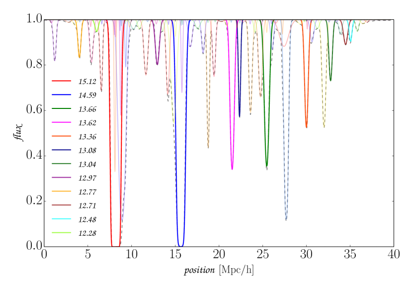
Figure 1: Showing absorber decomposition for a single skewer through our simulation box. The coloured curves show all the absorption lines fitted to the original simulation spectrum (shown in black dashed line). Twelve absorption profiles have been emphasized, spawning almost the full range of column densities probed. For those twelve, the colour coded legend displays their $\log_{10}(N_{\rm HI})$, using $\mathrm{cm^{-2}}$ units.

The spatial positions, column densities, and line widths from these fits are used for $f(N_{\rm HI})$ and to test our $W(x|N_{\rm HI})$ model. They are also used to construct simplified mocks in addition to the full simulations. In particular, in addition to the simulation Ly$\alpha$ forest sightlines, this study uses two simplified mock catalogues:

mocks:

These spectra use the line catalogue from fitting the simulation to reconstruct spectra, but substitutes the Absorber Model linewidth, $W(x|N_{\rm HI})$ (and discussed shortly) for the simulated linewidth. This simplification is helpful for testing our model.

random mocks:

Same as mocks except the positions of all lines have been randomly scrambled. This eliminates the correlations between separate absorbers, making the 2-absorber term zero.

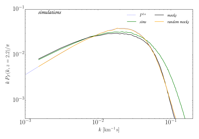
Figure 2: Comparison of the 1D flux power spectrum between spectra that are constructed from the simulation with different approximations. The green solid curve shows the power spectrum of the simulation spectra, and the black solid curve shows the power spectrum of the mocks spectra. The mocks used the fitted positions and columns in the simulations but substitute our simple linewidth model. The orange solid curve shows the power spectrum of the random mocks, which are the same as the mocks except that the positions of the absorption features have been randomly scrambled to eliminate correlations. See Section 3.1 for additional description. The blue dotted curve is the model 1-absorber contribution. Up to sample variance in the simulation, this analytic 1-absorber calculation should be identical to the random mocks prediction.

The differences between the full simulations (denoted sims in plots) and these simplified mocks are instructive for understanding what drives correlations. At our fiducial redshift of $z=2.2$, the full simulation spectra have $\tau_{\rm eff}=0.160$ and the mocks spectra (which use our line model) have $\tau_{\rm eff}=0.169$. As alluded to earlier, we find that randomizing the positions of absorbers in the simulations results in sub-percent differences in $\tau_{\rm eff}$ (at $z=2.2$). Additionally, Fig. 2 shows the changes in the power spectrum of the normalized flux overdensity between the full simulation (sims) and the same, but substituting our line-width model (mocks). Most of the differences in the power spectrum between the sims and mocks lies in the thermal cut-off at high wavenumbers. We believe this occurs because the sims capture the scatter in line widths at fixed $N_{\rm HI}$, while the mocks assume a one-to-one correspondence between the two given approximately by the mean relation. However, the large-scale behavior of the power spectrum is only altered at the few percent level between sims and mocks, suggesting that the line width model is less important there.

The yellow solid curve in Fig. 2 is the flux power spectrum obtained from the random mocks. The random mocks power spectrum is more discrepant with the sims and mocks power spectra. This indicates that the correlations between distinct absorbers have some effect on shaping the Ly$\alpha$ forest power spectrum. We note that, up to sample variance, the random mocks power spectrum should be identical to the 1-absorber term in our model. This result is confirmed in Fig. 2 by comparing the yellow solid random mocks curve with the blue dotted 1-absorber curve (which is calculated from solving our Eq. 2.16 and the same line width model).

3.2 Absorber properties in models

The simulation’s line catalogue plus simple analytic models are used to construct the inputs for the Absorber Model. Here we describe each input:

column density distribution:

The column density distribution function, $f(N_{\rm HI})$, is tabulated from our simulation’s absorber catalogue. Note that the simulations largely miss $N_{\rm HI}\gtrsim 10^{17}\;\mathrm{cm^{-2}}$ because they do not have self-shielding; this does not affect our comparison between the simulations and the Absorber Model, but does result in the calculations in this paper missing the not-insignificant contamination from high-$N_{\rm HI}$ absorbers [76, 77, 78, 79, 80].

line profile:

We assume that $W(x|N_{\rm HI})$ is Gaussian with standard deviation $\sigma_{a}(N_{\rm HI})$. To model $\sigma_{a}$, we use a model based on that presented in [81]. This model uses the correspondence between the column density $N_{\rm HI}$, gas over-density $\Delta_{b}$, and gas temperature $T$ found in simulations [82, 83] and that applies to the extent that the size of absorbers is set by the Jeans length [63] and that the temperature follows a $T-\Delta$ relation [84, 85]. Additionally, this model makes the ansatz that the velocity broadening is set by applying Hubble’s law across the Jeans length extent of the absorbers. This velocity broadening plus thermal Doppler broadening are added in quadrature to set the linewidth. (The velocity broadening is really determined by the nonlinear velocity field; however, at the low densities where Hubble broadening likely dominates over thermal Doppler, this Hubble-broadening approximation is more relevant.) This model captures the mean of the distribution of linewidths in simulations [81]. The model ignores the wide dispersion in linewidths at fixed column, although this dispersion appears to primarily affect the 1D power spectrum near the thermal cutoff (compare sims and mocks curves in Fig. 2; the mocks uses this line model). See Appendix B for more details on this line model. Finally, we assume that $T=T_{0}\Delta_{b}^{\gamma-1}$, with $T_{0}=12,300\;\mathrm{K}$ and $\gamma=1.59$ to match our simulations at $z=2.2$.

linear bias

: Our model for the absorber bias is based on a one-to-one matching of a Lagrangian region with linear overdensity $\delta_{L}$ with a Lagrangian region that results in a column of $N_{\rm HI}$ and Jeans-length physical size $\lambda_{J}(N_{\rm HI})$, with this matching ordered in increasing $\delta_{L}$ and $N_{\rm HI}$. However, in reality not all gas is accounted for in our fits to the column density distribution. Systems that contribute weak absorption are missed because of incompleteness of the line fitting as well as because the absorption-line description breaks down for extremely diffuse gas. Systems in dense regions are missed, for one, because $\Delta_{b}\sim 100$ gas tends to shock heat at virialization and, hence, not host significant neutral hydrogen. Because the missing gas tends to be at the lowest and highest densities that have the large absolute bias factors, we find that accounting for these missing contributions is important in order for the Absorber Model to match the large-scale power spectrum.

Therefore, we define parameters $\epsilon_{<}$ and $\epsilon_{>}$ that account for the breakdown of this one-to-one mapping at low and high columns (see Appendix C for more details). We find that setting $\epsilon_{<}=10^{-2}$ eliminates the divergence to large negative biases that appears for much smaller $\epsilon_{<}$, and that the results are stationary when changing $\epsilon_{<}$ by a factor of several around this value. Thus, in our bias models we fix $\epsilon_{<}=10^{-2}$ and we adjust $\epsilon_{>}$. The fraction of highly biased material that is not accounted for by our column density distribution is given by $\epsilon_{>}/(1.5+\epsilon_{>})$ at $z=2.2$ (Appendix C). Simulations show that $20\%$ of the gas in the Universe shock heats to $T>10^{5}$K [86], collisionally ionizing much of the neutral hydrogen, and relatedly, at $z=2.2$, $20\%$ of the gas is in $>10^{10}M_{\odot}$ dark matter halos that are able to pull in gas and form galaxies. Thus, our rough expectation is that $20\%$ of dense gas is likely “missing” in our column density distribution, meaning $\epsilon_{>}/(1.5+\epsilon_{>})\sim 0.2$ or equivalently $\epsilon_{>}\sim 0.5$. We find in Section 4.2 that $\epsilon_{>}=0.5-1$ is needed to match the large-scale power in the simulations, with the exact value depending on the absorber exclusion model. Figure 9 in Appendix C shows that for $\epsilon_{>}=0.9$ the Eulerian absorber bias ranges from $b(N_{\rm HI})\approx-0.5$ at $N_{\rm HI}=10^{11-12}$cm^-2 to $b(N_{\rm HI})\approx 0.8$ for $N_{\rm HI}=10^{14.5-17}$cm^-2 (with the latter tending to $b(N_{\rm HI})\approx 1.1$ if we instead take $\epsilon_{>}=0.4$).

In this paper we also assume that the linear gas density is a windowed version of the linear total matter density due to pressure smoothing, such that $P_{b}=P_{L}e^{-k^{2}/k_{F}^{2}}$ where $P_{b}$ and $P_{L}$ are the linear gas power spectrum and linear total matter power spectrum, respectively, and $k_{F}=2\pi/\lambda_{F}$ is the filtering scale which we take to be $k_{F}^{-1}=0.041\;c\mathrm{Mpc}/h$ ([87, 88]; see the appendices for details). However, the Absorber Model flux power spectrum is insensitive to this $k_{F}$-windowing because the small-scale power is dominated by the 1-absorber term at the redshifts we have analyzed.

These choices complete the inputs needed to compute correlations in our model using Eqs. 2.15-2.17. In what follows, we calculate the power spectrum in the model and compare with the power spectrum from the simulation mocks.

4 The Ly$\alpha$ forest power spectrum

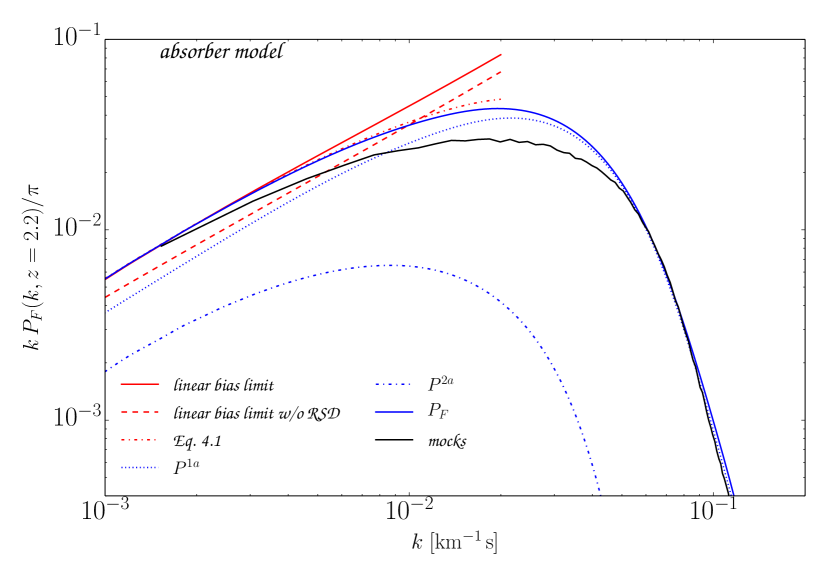
Figure 3: Flux power spectra as calculated in the simulation mocks (black solid curve) and in the Absorber Model (blue curves). The Absorber Model is decomposed into contributions from the 1-absorber term (blue dotted curve), the 2-absorber term (blue dot-dashed curve), and their total (blue solid curve). The red solid line shows the large-scale limit of the Absorber Model using Eq. 4.2, the red dashed line shows the same but without redshift-space distortions, and the dot dashed curve shows this calculation keeping the scale dependence of $N_{p}^{-1}$.

Now that we have all the ingredients needed to compute the correlations in our model, we focus on the line of sight (or 1D) flux power spectrum. Fig. 3 show the different components that contribute to the absorber power spectrum. Respectively, the 1-absorber, 2-absorber, and full power spectrum were calculated by taking the Fourier transform of Eq. 2.16, Eq. 2.17 and Eq. 2.15, with the models for $f(N_{\rm HI})$, $W(x|N_{\rm HI})$, and $b(N_{\rm HI})$ specified in the previous section. The overall shape of the Absorber Model power spectrum agrees to $\sim 20\%$ with the mock spectra, with the best agreement on the small scales that are determined by the 1-absorber term and the worst at intermediate scales. Since we are comparing to the mocks, and not the original simulations, the only two effects that can change the behavior of the flux power at those scales is non-linear clustering and the related positional ‘exclusion’ of absorption lines (discussed shortly).

Interestingly, the 1-absorber term is at least three times larger than the 2-absorber term, with the difference increasing with wavenumber. On scales much larger than the linewidth, the 1-absorber power spectrum is white. This has a couple interesting implications. First, mode counting arguments for the constraining power of the Ly$\alpha$ forest have missed this source of noise, and previous attempts to use the 1D power to measure the bias of the transmitted flux have overestimated the bias because of the 1-absorber term [79, 6].

Let us understand the large-scale limit of the power spectrum. At large-scales $\xi_{F}=\exp[\xi_{\tau}^{1a}+\xi_{\tau}^{2a}]-1$ can be expanded to yield $\xi_{F}\approx\exp[\xi_{\tau}^{1a}](1+\xi_{\tau}^{2a})-1$, or taking the Fourier transform:

$$P_{F}(k)=P_{\tau}^{2a}(k)+P_{F}^{1a}(k)+P_{\tau}^{2a}(k)\star P_{F}^{1a}(k),$$ (4.1)

where $P_{F}^{1a}(k)$ is the power spectrum of $\xi_{F}^{1a}=\exp[\xi_{\tau}^{1a}]$ (Eq. 2.16), which asymptotes to a constant at low $k$, and $P_{\tau}^{2a}$ is the Fourier transform of $\xi_{\tau}^{1a}$ (Eq. 2.17). The last term in Eq. 4.1 is just a few percent of the total power at all wavenumbers, and, if it is dropped, we can rewrite Eq. 4.1 as

$$P_{F}(k)\approx\int_{k}^{\infty}\,dq\,q\,P_{m}^{3D}(q)\left(b_{F,\delta}+fb_{F,\eta}\mu^{2}\right)^{2}+N_{P}^{-1},$$ (4.2)

where $\mu=k/q$ is the angle between the line of sight and the Fourier vector $\vec{q}$, and the linear bias factors for the density ($b_{F,\delta}$) and velocity gradient ($b_{F,\eta}$) are given by the relations in Sec. 2.1. The $k$-independent Poissonian term, $N_{P}^{-1}\approx P_{F}^{1a}(k\rightarrow 0)$, is dominated by the Poisson 1-absorber term. In the $\tau_{\rm eff}\ll 1$ limit, the shot-noise term is related to the effective optical depth through Eq. 2.20. The solid red line in Fig. 3 is the evaluation of Eq. 4.2 for our model, where all the non-convolution terms of 2-absorber power (which have a white power as $k\rightarrow 0$) were kept in $N_{P}^{-1}$. If we keep the scale dependence of $N_{P}^{-1}$, the result (the dot-dashed red curve) deviates significantly from the red solid line only at $k\gtrsim 0.01\,\mathrm{s\,km^{-1}}$ and is only 12% larger at $k=0.02\,\mathrm{s\,km^{-1}}$ than the full model flux power (full blue line in Fig. 3). The approximation of Eq. 4.2 but with $b_{F,\eta}=0$ is shown as dashed red line in Fig. 3, showing that redshift-space distortions shape the power at the 20% level (contributing at ${\cal O}(0.4)$ level to the 2-absorber term in the Reference Model).

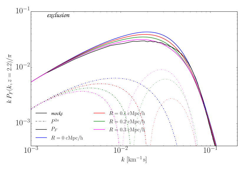
Figure 4: The effect of absorber exclusion on the flux power spectrum. The black solid curve corresponds to the results of the simulation mocks, while different colored curves correspond to setting $\xi_{12}(x)=-1$ at $x<R$, with $R=0$ (in blue) being the Reference model. The colored solid curves show the total flux power in the absorber model, while the dot-dashed curves with corresponding color shows the contribution from the 2-absorber term only. The translucent curves indicate regions of negative 2-absorber power. For all models, the bias has been tuned to match the large-scale limit of the mocks.

4.1 Absorber exclusion

Absorbers’ positions can be anti-correlated on small scales owing to absorbers having to occupy different real space positions – absorber exclusion. We show that absorber exclusion is likely the reason why our Reference Model, which does not include exclusion, overpredicts the 1D power spectrum at intermediate wavenumbers.

We illustrate exclusion with a simple model in which we remap the absorber correlation function in the 2-absorber term (Eq. 2.17) to

$$\xi_{12}^{L}(x)\rightarrow\begin{cases}-1&\mbox{if }0<x<R;\\ b_{1}b_{2}\xi_{L}(x)&\mbox{if }x\geq R,\end{cases}$$ (4.3)

where $\xi_{L}$ is the usual linear matter correlation function. While we have not included redshift-space distortions in the above, really for $x\geq R$ we include these terms but set them to zero at $x<R$ (so that our exclusion happens in redshift space). Figure 4 shows the effect of exclusion on the 1D power spectrum. The different curves vary $R$ by up to a few times the Jeans length at $z=2.2$ ($\lambda_{J}\sim 0.05\,c\mathrm{Mpc}/h$; Eq. B.8). The Jeans length is the characteristic size of absorbers. (Analogously, to explain the sub-Poissonian shot noise found in halo clustering, halo exclusion is found to become important below a few times the virial radius [55].) The $R=0\,c\mathrm{Mpc}/h$ model is our Reference Model, which does not include exclusion. While $R=0.3\;c\mathrm{Mpc}/h$ works well on large scales, matching the mocks on small scales requires a smaller value of $R$ (see Fig. 4), a trend likely reflecting the simplicity of the exclusion model used.

Additionally, the absorber exclusion suppresses the large-scale power in the model by reducing the shot noise. The actual effect is coming from a modified 1D matter power spectrum. For a simple model of line exclusion considered in this paper, an analytic relation can be obtained such that

$$P_{12}(k;R)=P_{12}(k;R=0)-2R\,W_{R}(k)-2R\,\left[P_{12}\star W_{R}\right](k),$$ (4.4)

where $P_{12}(k)$ is the Fourier transform of $\xi_{12}^{L}$ and $W_{R}(k)=\sin(kR)/(kR)$ is a 1D Fourier transform of a top-hat function and $R$ is the exclusion scale. In the large-scale limit, $k\rightarrow 0$, the correction due to absorber exclusion in the flux power spectrum can be written as

$$P_{F}^{2a}(k;R)=P_{F}^{2a}(k;R=0)-\lambda\,R,$$ (4.5)

and $\lambda=0.09$ in our model. The convolution term from exclusion in Eq. 4.4 adds less than 4% of the total value of $\lambda$. However, the overall effect of exclusion is quite large: in Eq. 4.5, $\lambda\,R$ is 75% of $P_{F}^{2a}(R=0)$ for $R=0.3\;c\mathrm{Mpc}/h$.

Fig. 4, however, does not show the large-scale suppression of power from exclusion. Since this effect is perfectly degenerate with the choice of large-scale absorber bias, $b_{F,\delta}$, and we take that effect out of the calculation by changing the biasing scheme. To match the large-scale limit, the adjusted bias values for $R=0.1,~{}0.2$ and $0.3\;c\mathrm{Mpc}/h$ are $b_{F,\delta}=-0.09,\,-0.1$ and $-0.11$ respectively. This should be compared to the value of bias in the Reference Model, $b_{F,\delta}=-0.08$.

4.2 Absorber bias

In our simple model of absorber bias we can vary two parameters, $\varepsilon_{>}$ and $\varepsilon_{<}$, to match the large-scale bias in the mocks spectra (see Appendix C). Of these, $\varepsilon_{>}$ is the most important, representing the amount of highly biased material that does not contribute to the forest absorption (because of, e.g., shock heating). In our Reference model, these parameters were chosen to be $(\varepsilon_{<},~{}\varepsilon_{>})=(0.01,0.9)$ such that the large-scale 1D flux power spectrum of the model agrees with the results from the simulation mocks at $z=2.2$. Here we investigate the impact of varying $\varepsilon_{>}$. We show $\varepsilon_{>}=\{0.9,~{}0.7,~{}1.3\}$ in Fig. 5, which respectively result in $b_{F,\delta}=-\{0.080,~{}0.105,~{}0.063\}$. Thus, varying $\varepsilon_{>}$ over this range results in a small change in $b_{F,\delta}$ and, as a result, small changes in the large-scale power. The model with $\varepsilon_{>}=0.9$ is most consistent with the mocks power. This is consistent with the $\varepsilon_{>}=0.5-1$ we motivated in Section 3.2 (from considering gas ‘lost’ to shock heating and galaxy formation), and we note that the models with exclusion that match the bias require $\varepsilon_{>}=0.71,~{}0.57,$ and $0.46$ for $R=0.1,~{}0.2$ and $0.3\;c\mathrm{Mpc}/h$ respectively. Thus while a certain degree of tuning was performed on the bias to match the large scale limit of the mocks power, the chosen parameter values lie well within the reasonable assumption of the simple bias model used. We suspect improved models for the absorber bias and absorber exclusion can be developed, models for which less tuning is required.

Since we find a best fit flux bias of $b_{F,\delta}=-0.08$, this translates into the effective bias of the absorption lines, $-b_{F,\delta}/\tau_{\rm eff}$ (c.f. Eq. 2.22), of approximately $0.5$, using $\tau_{\rm eff}=0.16$. This is approximately the model bias of $N_{\rm HI}\sim 10^{14}~{}$cm^-2 systems that Section 4.4 shows dominate the 2-absorber correlations.

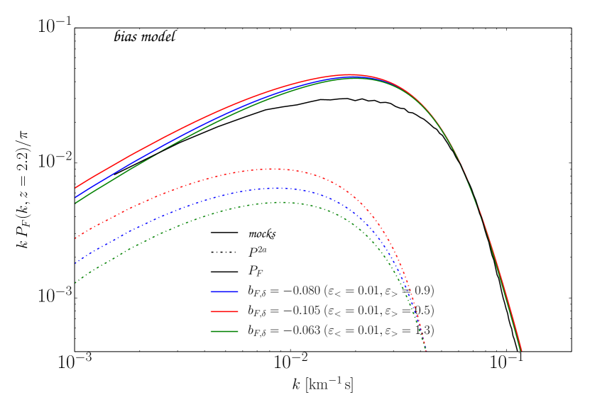
Figure 5: The effect of varying the parameters of our bias model on the 1D flux power spectrum. Different colored curves have varied our simple bias model’s two free parameters, $(\varepsilon_{>},\varepsilon_{<})$, with solid indicating the total power and the dot-dashed indicating the 2-absorber contribution. The full black curve corresponds to the results of the simulation mocks.

4.3 Redshift evolution

The amplitude of the 1D Ly$\alpha$ forest power spectrum increases significantly with redshift, and constraints on cosmological parameters derive a lot of their sensitivity from having measurements at multiple redshifts. Thus, it is interesting to consider our model at a higher redshift to determine whether it captures the expected trends. We again compare the Absorber Model with the mocks spectra (which share the same linewidth model), but these spectra are now constructed using the $z=3.0$ simulation output. We also use the same bias parameters $(\varepsilon_{>},\varepsilon_{<})$ as the $z=2.2$ Reference Model.

Fig. 6 compares the flux power spectra of the Absorber Model and mocks for both $z=2.2$ (lower curves) and $z=3.0$ (upper curves). By and large, the $z=3.0$ curves all are shifted up by a comparable factor in amplitude compared to the $z=2.2$. Thus, our previous conclusions apply: The 1-absorber term is similarly dominant. The effect of clustering is similar, albeit somewhat larger at $z=3.0$. The ratios of the total power, 1-absorber power, and 2-absorber power at $k=10^{-3}\;\mathrm{s\,km^{-1}}$, are $1$ : $0.66$ : $0.32$ at $z=2.2$ and $1$ : $0.57$ : $0.40$ at $z=3$. (The convolution term in Eq. 4.1 is 1% and 2% of the large-scale power at $z=2.2$ and $3.0$, respectively.) The Absorber Model is slightly more discrepant with the mocks at $z=3.0$, overpredicting the large-scales power by $\approx 15$%. While our bias model was tuned to match large-scale properties at $z=2.2$, we have not tuned parameters for $z=3.0$. Indeed, we find that decreasing the value of $b_{F,\delta}$ in the model by $30$% matches the large-scale power in the mocks at $z=3.0$.

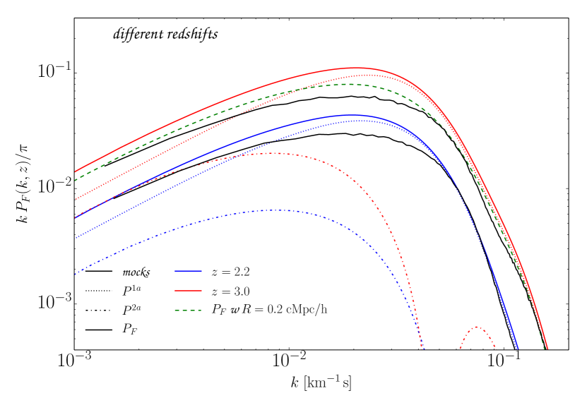
Figure 6: Comparison of 1D flux power spectrum at $z=2.2$ (in blue) and $z=3.0$ (in red). The blue and red solid curves show the total flux power spectrum in the Absorber Model, while the dotted and dot-dashed lines show contribution from 1-absorber and 2-absorber terms, respectively. The black solid curves shows the results of the simulation mocks, with the $z=2.2$ case below $z=3.0$. The green dashed curve shows at $z=3$ model with line exclusion below $R=0.2\;c\mathrm{Mpc}/h$.

Both observations [10, 11] and simulations [6, 71] suggest redshift evolution to be power-law with redshift, with the power-law index of slightly less than $3$ ($b_{F,\delta}\propto(1+z)^{2.9}$). The results of the Absorber Model suggest a redshift evolution closer to a power-law index of $2$ ($b_{F,\delta}\propto(1+z)^{2}$), with the caveat that this scaling is likely affected by the thermal history. Using the $30$% lower value of $b_{F,\delta}$ suggested by the large-scale limit of the $z=3.0$ mocks power would further increase the discrepancy with the observed power-law index. Increasing the amount of absorber exclusion with redshift could help reconcile this discrepancy. (Fixing the large-scale power results in $\approx 30\%$ larger $b_{F,\delta}$ to compensate for exclusion with $R=0.2\;c\mathrm{Mpc}/h$. The green solid curve in Fig. 6 shows our $R=0.2\;c\mathrm{Mpc}/h$ toy exclusion model but with the same $b_{F,\delta}$.) Larger model biases could also be created by decreasing $\varepsilon_{>}$, which is theoretically motivated as only half the gas has shocked heated or collapsed into galaxy-sized halos at $z=3$ compared to $z=2.2$ ([86]; suggesting a similar reduction in $\varepsilon_{>}$). Thus, the discrepancy at large scales at $z=3.0$ falls within the plausible range of input parameters to the Absorber Model.

4.4 Column densities

The Absorber Model describes the Lyman-$\alpha$ forest by discretizing it into systems of different columns. This discretization allows us to understand which systems are most important in shaping the correlations. Fig. 7 shows the predictions of the Absorber Model when making different cuts on column density. The Reference Model (the blue curve) uses the range between $11\leq\log_{10}(N_{\rm HI})\leq 17$, using cm^-2 units. When excluding the low column densities from the calculation with $\log_{10}(N_{\rm HI})<13$ (solid red curve), the flux power spectrum is reduced by $13\%$ on large scales. However, the small-scale power is nearly unchanged. Excluding low columns also has little effect on 1-absorber term, whereas the 2-absorber term is reduced by a factor of several when excluding the columns below $\log_{10}(N_{\rm HI})=13$ (red lines). Excluding the high column densities with $\log_{10}(N_{\rm HI})>15$ also mostly affects large scales. However, for this case, the 1-absorber term is most changed, being reduced by $17\%$.

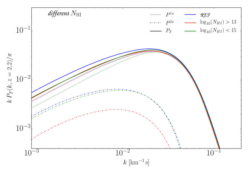
Figure 7: Absorber model power spectrum for different column density cuts. The solid curves show the total flux power, the dot-dashed curves show the 2-absorber term, and the dotted curves show the 1-absorber term. The Reference Model is in blue, which includes all columns, $11\leq\log_{10}(N_{\rm HI})\leq 17$. The flux power excluding low column densities is shown in red, and the flux power excluding high column densities in green.

All Absorber Model quantities can be expressed as

$$X=\int_{-\infty}^{\infty}\frac{\partial X}{\partial\log_{10}(N_{\rm HI})}d\log_{10}(N_{\rm HI}),$$ (4.6)

where $X=\{\tau_{\rm eff},P_{F}^{1a},P_{F}^{2a},\dots\}$. Thus, $\partial X/\partial\log_{10}(N_{\rm HI})$ gives the contribution to $X$ per $\log_{10}(N_{\rm HI})$. Fig. 8 shows $\partial X/\partial\log_{10}(N_{\rm HI})$ over the column density range probed by the simulations. The flux power spectrum components depend also on the wavenumber. Our calculations take $k=10^{-3}\mathrm{s\,km^{-1}}$, or $\approx 0.1h\,\mathrm{Mpc^{-1}}$, at $z=2.2$, but the $X(N_{\rm HI})$ do not change significantly if $k$ is increased/decreased by a factor of ten. Additionally, the top axis in Fig. 8 relates the column to the gas density in units of the mean, using the relation from [63] that our model adopts.

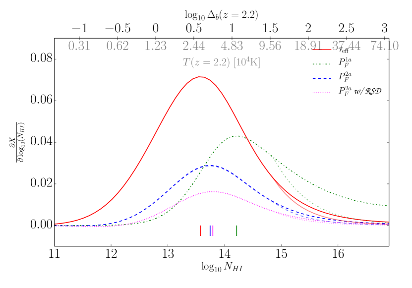
Figure 8: The differential of quantity $X$ with respect to column density, $\partial X/\partial\log_{10}(N_{HI})$, for $X=\tau_{\rm eff}$ (red solid curve), $X=P_{F}^{1a}$ (green dot-dashed curve), $X=P_{F}^{2a}$ (blue dashed curve), and $X=P_{F}^{2a}$ without redshift-space distortions (dotted magenta). The vertical markers (with the same colour scheme) at the bottom of the plot indicate the maximum of the different distributions. These contributions to the power spectrum were computed at the pivot scale of $\sim 0.1h\,\mathrm{Mpc^{-1}}$. The top axii show the gas density contrast $\Delta_{b}$ (above) and gas temperature $T_{g}$ (below) for our $z=2.2$ model. The corresponding translucent curves are if we instead take an upper limit on the temperature of $10^{5}\;\mathrm{K}$, which mimics a more realistic thermal model.

The effective optical depth distribution, $\partial\tau_{\rm eff}/\partial\log_{10}(N_{\rm HI})$, and the 2-absorber term, $\partial P_{F}^{2a}/\partial\log_{10}(N_{\rm HI})$, peak at slightly lower columns of $10^{13.6}\;\mathrm{cm^{-2}}$ than the 1-absorber term, $\partial P_{F}^{1a}/\partial\log_{10}(N_{\rm HI})$, which peaks at $10^{14.2}\;\mathrm{cm^{-2}}$. These trends are consistent with the previously noted trends in the 1D power spectrum between different column density cuts (Fig. 7). (We also find that redshift-space distortions act to shift the peak of $\partial P_{F}^{2a}/\partial\log_{10}(N_{\rm HI})$ towards lower columns.) In terms of densities, at $z=2.2$ $\tau_{\rm eff}$ comes from a the wide range of densities, $\Delta_{b}=0.3-30$, with a peak at $\Delta_{b}\approx 4$. The range of densities affecting the 2-absorber signal is shifted to somewhat higher densities, with a peak at $\Delta_{b}\approx 5$, and the distribution is somewhat less broad ($\Delta_{b}=0.7-10$). Finally, the 1-absorber term peaks at $\Delta_{b}\approx 10$, and most of its contribution comes from between overdensities of several and halo-like overdensities.

The contribution for the 1-absorber term is skewed in the direction of higher column densities. However, some of this skewness owes to unrealistically high gas temperatures in the model from extrapolating a temperature density relation to densities beyond where it applies (see top temperature axis in Fig. 8), leading to unrealistically large linewidths. The translucent lines in Fig. 8 show how the tail of the 1-absorber contribution is diminished when the gas temperature is limited to be below $10^{5}\;\mathrm{K}$, a limit that physically comes about from collisional cooling [89, 85]. While other terms change negligibly, the Poisson term now falls much faster towards zero contribution at higher columns. Nevertheless, the 1-absorber term is sensitive to temperatures of the gas at column densities of around $10^{14}-10^{15}\;\mathrm{cm^{-2}}$, even if we cap the temperature to mimic more realistic thermal physics. Moreover, with the inclusion of column densities that are in the self-shielded regime (LLSs and DLAs), the 1-absorber term’s distribution likely develops a second peak at high columns (when $f(N_{\rm HI})$ flattens out, and ${\mathrm{E}W}(N_{\rm HI})$ starts increasing with $\sim\sqrt{N_{\rm HI}}$ owing to damping wing absorption).

For $z=3.0$, the same column density corresponds to a lower overdensity than at $z=2.2$. Interestingly, we find that $\partial\tau_{\rm eff}/\partial\log_{10}(N_{\rm HI})$ and $\partial P_{F}^{2a}/\partial\log_{10}(N_{\rm HI})$ peak at similar gas overdensities at $z=2.2$ and $z=3.0$, meaning that these are shaped by similar gas densities but by higher column densities with increasing redshift. Whereas, we find that $\partial P_{F}^{1a}/\partial\log_{10}(N_{\rm HI})$ peaks at similar column densities at both redshifts, meaning that this term is shaped by lower gas overdensities at higher redshifts.

5 Conclusion

This paper presented a semi-analytic ‘Absorber Model’ for the Ly$\alpha$ forest that is inspired by the Halo Model. This model is built on the absorption line decomposition of the Ly$\alpha$ optical depth field, a decomposition that has been used since the dawn of high-resolution Ly$\alpha$ forest observations. This decomposition allows one to break up correlations into those within each absorption system (‘the 1-absorber term’) and those between systems (‘the 2-absorber term’), treating these systems as biased tracers of the underlying matter fluctuations. While the nonlinear exponential mapping between optical depth and flux requires an infinite series of moments to calculate any statistic, we show that this series can be re-summed (capturing the Poissonian 1-absorber term at all orders and truncating the 2-absorber at the desired order in $\delta_{L}$).

We have focused on using this model to understand Ly$\alpha$ forest two-point correlations, where we found:

• The modeled line-of-sight flux power spectrum (also known as the 1D power spectrum) agrees well with that in simulations. For this comparison, we matched the column density distribution and linewidths in the model and the simulation mocks. The primary additional ingredient that the model requires is the linear bias as a function of $N_{\rm HI}$, and we showed that a minimalist model predicts biases consistent with the simulations. In addition, we showed that a simple linewidth model based on the model in [81] reproduced many aspects of the 1D power spectrum. Absorber exclusion on the scale of the IGM Jeans length is needed to suppress the model’s power by 30% at intermediate wavenumbers to match the simulations.

• The 1-absorber contribution to the 1D power spectrum is a factor of few times larger than the 2-absorber contribution (at least for the redshift range considered here of $z=2-3$). The largeness of the 1-absorber term indicates that the 1D power at all wavenumbers is primarily shaped by the number of absorbers as a function of column. To the extent that the sensitivity to cosmological parameters enters via the 2-absorber term, the 1-absorber term – which is a single number on scales much larger than the linewidths – acts as a source of effective noise. The dominance of Poisson fluctuations also helps explain why [90, 82] found that large-scale temperature and intensity fluctuations have little effect on the 1D power spectrum.

• We derived intuitive formulae for the effective optical depth and the $k\rightarrow 0$ limits of the 1- and 2-absorber terms, showing that they can be expressed simply as different equivalent-width weightings of the column density distribution (with an additional bias factor in the 2-absorber term’s weighting). At $z=2.2$, we found that the 2-absorber term is dominated by systems with $N_{\rm HI}\sim 10^{13}-10^{15}\;\mathrm{cm^{-2}}$, while the 1-absorber term derives from those with $N_{\rm HI}\sim 10^{14}-10^{15}\;\mathrm{cm^{-2}}$. Moreover, irrespective of redshift, the 1-absorber contribution traces these same column densities, whereas the 2-absorber contribution traces the same gas overdensities, peaking at overdensities of $\sim 5$ and spanning $\sim 0.7-10$.

• This is the first model that successfully predicts the Ly$\alpha$ forest linear biases in both density and velocity. An objection to this claim might be that we have just redefined the uncertainty into $b(N_{\rm HI})$, but a counterargument is that $N_{\rm HI}$ tightly correlates with density [63, 82, 83] and so a simple biasing model is possible. Our simplest model for the linear velocity gradient bias, $b_{F,\eta}$, finds that it should equal $\tau_{\rm eff}$. Our full model finds that peculiar velocity broadening contributes an additional 10-20% correction that brings $b_{F,\eta}$ into agreement with simulations.

The Absorber Model has several deficiencies. A major one is the unnatural splitting of correlations into those within systems and between systems, a problem that any halo-like model encounters. Absorber exclusion is one manifestation of this unnaturalness, which acts to suppress the 1-absorber term on large-scales, but really appears in our 2-absorber term. Another example is the pressure smoothing of the gas, which both changes the profile of absorbers (affecting mainly the 1-absorber term) and also likely alters the absorber spacing (affecting the 2-absorber). Our calculations mostly punted on modeling these ‘filtering’ effects. Perhaps the most significant deficiency is that, in contrast to the Halo Model, which is built upon the solid foundation of excursion set theory [91] and the attractor NFW halo profile [92], the Absorber Model requires the column density distribution (we took fits to it from simulations) as well as models for the linewidth distribution and the line density bias. The column density distribution itself is ambiguously defined, as at some level the forest cannot be decomposed into discrete systems. This drawback should be especially prescient at $z>4$, where much of the forest is saturated, and we expect the Absorber Model will not be as successful. On the positive side, the densities and linewidths as a function of column have been studied and there is some analytic understanding of both. Our line model was able to build off this understanding to develop simple models for, e.g., the bias of lines.

There are many possible extensions to this model, including

• Computing the model predictions at higher order in $\delta_{L}$ than second order, which in detail would require pursing a bias expansion for the absorbers [e.g. 93] or using some other model for the absorbers’ nonlinear clustering. (When the 2-absorber term is exponentiated, our formulae for moments of the flux field contain terms at every order in $\delta_{L}$, but they are only complete at second order.) At second order in $\delta_{L}$, our model does not appear to capture the nonlinear scaling of the 3D flux power spectrum found in [6, 71]. The 1-absorber term will likely be subdominant in the 3D power spectrum as it scales as $k^{3}$, and so the nonlinear scaling found in [6, 71] likely owes to aspects of the nonlinear absorber clustering that are currently not included in our model.

• Understanding how the shapes of correlations in the Ly$\alpha$ forest depend on the underlying cosmology. To the extent that the 2-absorber term dominates cosmological parameter constraints, the calculations presented here provide some understanding. However, the small-scale width of absorption features should bear some cosmological dependence (that may be distinct from thermal effects), and the column density distribution also should depend on the cosmology. These dependencies were not captured in our simplified calculations.

• Including the damping wings of high-column density systems (Lyman-limit and damped Ly$\alpha$ systems). This addition is a matter of simply including natural broadening in our linewidth model. Several studies have shown that the effect of the wings on the power spectrum can be significant [76, 77, 78, 79, 80]. This model could potentially provide a physically-motivated parametrization for their effect.

• Including metal absorption that contaminates the Ly$\alpha$ forest. This could again be incorporated by altering the linewidth model to include absorption by various metal ions given some mapping between $N_{\rm HI}$ and the ions’ optical depth profile. A sophisticated model could assume some metallicity distribution as a function of column (as this has been constrained observationally [94, 95, 96]) and use photoionization modeling to include all potentially contaminating absorption lines. Such a model for metal contamination could aid in understanding the imprints of metal contamination on the forest and how this contamination could bias parameter inferences. Similar calculations could be used to study the cross-correlation between the Lyman-$\alpha$ forests and the absorption in other lines (such as the Ly$\beta$ or C IV forests).

State-of-the-art Lyman-$\alpha$ forest studies rely heavily on cosmological hydrodynamic simulations. The Absorber Model is a complementary semi-analytic approach that makes some analytic Ly$\alpha$ forest investigations possible. Additionally, a Monte-Carlo realization of this model could provide a more physical mock Ly$\alpha$ absorption catalogue than the popular method that uses lognormal transformations.

Appendix A Absorber model through Poisson distribution

Before we chose our discretization such that $p_{i}$ is either zero or one in a cell. Of course, to the extent that absorbers are uncorrelated (which is what the Absorber Model assumes on small scales), $p_{i}$ is Poissonian, as the absorbers are discrete. Using that they are Poissonian allows us to re-sum all Poissonian terms in the $\tau$ expansion expansion, as opposed to our approach in the main text of keeping track of terms to third order in $\tau$ and then motivating the resummation. Keeping the notation adopted in Section 2, we can rewrite the optical depth from Eq. 2.1 such that each $\tau_{i}=\tau_{a}(x-x_{i}|N_{i})$ in the sum over a grid of $\Delta N$ and $\Delta x$ is multiplied by the occupation number of elements ($n_{i}$), corresponding to $(N_{i},x_{i})$ within that volume

$$\tau(x)=\sum_{i}n_{i}\tau_{i}.$$ (A.1)

The random variable $n_{i}$ is Poisson distributed with average

$$\langle n_{i}\rangle\equiv{\bar{n}}(x_{i}|N_{i})=f(N_{i})\Big{(}1+\delta_{a}(x_{i}|N_{i})\Big{)}\Delta N\Delta x,$$ (A.2)

where $\delta_{a}$ is the overdensity of absorbers. [For linear configuration-space biasing, $\delta_{a}(x_{i}|N_{i})=b(N_{i})\delta_{L}(x_{i})$.] Because $\delta_{a}$ is not Poissonian, this means that even though we have assumed $n_{i}$ is Poissonian in each cell, the spatial distribution of absorbers is not owing to $\delta_{a}$. We note that we are making the same assumptions as in the main text, which follows the more standard approach. With this, we can write the flux of one absorber at position $x$ as

$$F(x)=e^{-\tau(x)}=e^{-\sum_{i}n_{i}\tau_{i}(x)}=\prod_{i}e^{-n_{i}\tau_{i}}\equiv\prod_{i}F_{i}.$$ (A.3)

To compute the mean of the flux requires averaging over the number the Poisson distribution of the number densities as well as over $\delta_{a}$:

$$\langle F\rangle=\left\langle\left\langle F(x)\right\rangle_{n}\right\rangle_{\delta}=\left\langle\left\langle\prod_{i}F_{i}\right\rangle_{n}\right\rangle_{\delta}=\left\langle\prod_{i}\left\langle F_{i}\right\rangle_{n}\right\rangle_{\delta}.$$ (A.4)

The average over the Poisson distribution can be done analytically and yields

$$\langle F\rangle= \left\langle\prod_{i}\sum_{n_{i}=0}^{\infty}P(n_{i}|{\bar{n}})e^{-n_{i}\tau_{i}}\right\rangle_{\delta},$$

$$= \left\langle\prod_{i}e^{{\bar{n}}(x_{i}|N_{i})\left(e^{-\tau_{i}(x)}-1\right)}\right\rangle_{\delta},$$

$$= \left\langle e^{\sum_{i}{\bar{n}}(x_{i}|N_{i})\left(e^{-\tau_{i}(x)}-1\right)}\right\rangle_{\delta}.$$ (A.5)

Using the expression for the average number density (Eq. A.2), and again changing the sum $\sum_{i}\rightarrow\int\frac{dN_{i}dx_{i}}{\Delta N\Delta x}$ yields

$$\langle F\rangle= \left\langle e^{\int dN_{1}\int dx_{1}f_{1}\left(1+\delta_{a}(x_{1})\right)\left(e^{-\tau_{1}(x)}-1\right)}\right\rangle_{\delta},$$ (A.6)

where we have replaced index $i$ with $1$ to match the notation in the main text (e.g. Eq. 2.10). Just as in Sec. 2, using the cumulant theorem we compute the $\delta$–average, which gives to quadratic order in $\delta_{L}$:

$$\langle F\rangle= \exp\left[\int_{N}d{\vec{N}}\int_{x}d{\vec{x}}f_{1}\left(e^{-\tau_{1}(x)}-1\right)+\right.$$

$$+ \left.\phantom{\int}\frac{1}{2}\int_{N}d^{2}{\vec{N}}\int_{x}d^{2}{\vec{x}}f_{1}f_{2}\xi^{L}_{12}(x_{2}-x_{1})\left(e^{-\tau_{1}(x)}-1\right)\left(e^{-\tau_{2}(x)}-1\right)\right],$$ (A.7)

where as in the main text $\langle\delta_{a}(x_{1})\delta_{a}(x_{2})\rangle=\xi_{12}^{L}(x_{2}-x_{1})$. With the replacement $\tau_{1}(x)\rightarrow\tau_{1}(y)+\tau_{1}(z)$, the above expression then becomes $\langle F(y)F(z)\rangle$, just as in Sec. 2.

Because this approach yields an expression for the flux given the large-scale density, $\delta_{a}$ (the term in the expectation value of Eq. A.6), it nicely allows one to compute the flux biases of the density ($b_{F,\delta}$) and of the velocity gradient ($b_{F,\eta}$). The density bias of the flux is defined as

$$b_{F,\delta}(k)\equiv\left\langle\frac{\partial\delta_{F}(k)}{\partial\delta_{L}(k)}\right\rangle=\frac{1}{\langle F\rangle}\left\langle\frac{\partial F(k)}{\partial\delta_{L}(k)}\right\rangle,$$ (A.8)

where the (constant) linear bias, which we denote as $b_{F,\delta}$ in the main text, is obtained by taking the ${k\rightarrow 0}$ limit. Using the above notation, $b_{F,\delta}(k)$ can be written as

$$b_{F,\delta}(k) =\frac{1}{\langle F\rangle}\left\langle\left\langle\frac{\partial F(k)}{\partial\delta_{L}(k)}\right\rangle_{n}\right\rangle_{\delta},$$

$$=\frac{1}{\langle F\rangle}\left\langle\frac{\partial}{\partial\delta_{L}(k)}\left\langle F(k)\right\rangle_{n}\right\rangle_{\delta},$$

$$=\frac{1}{\langle F\rangle}\left\langle\frac{\partial}{\partial\delta_{L}(k)}\int dxe^{-ikx}e^{\int dN_{1}f_{1}\int dx_{1}\left(1+b_{1}\delta_{L}(x_{1})+{\cal O}(\delta_{L}^{2})\right)\left(e^{-\tau_{1}(x)}-1\right)}\right\rangle_{\delta},$$ (A.9)

where for simplicity we have ignored redshift-space distortions in our expression as they do not alter $b_{F,\delta}(k)$.

To simplify further, we drop terms of ${\cal O}(\delta_{L}^{2})$ as these will yield zero in the desired $k\rightarrow 0$ limit (with a caveat discussed below) and consider a finite interval $L$ so we can write $\delta_{L}(x)=\sum_{n=-\infty}^{\infty}\delta_{L}(k)e^{ikx}\Delta k/2\pi$ where $\Delta k=2\pi/L$ and $k=n\Delta k$ for integer $n$. Then, rewriting the previous equation yields

$$b_{F,\delta}(k) =\frac{1}{\langle F\rangle}\left\langle\frac{\partial}{\partial\delta_{L}(k)}\int dxe^{-ikx}e^{-\int dN_{1}\int dx_{1}f_{1}\left(1+b_{1}L^{-1}\sum\delta_{L}(k^{\prime})e^{ik^{\prime}x_{1}}\right)\left(1-e^{-\tau_{1}(x)}\right)}\right\rangle_{\delta},$$

$$=\frac{-1}{\langle F\rangle}\left\langle\int dxe^{-ikx}e^{\int dN_{1}f_{1}\int dx_{1}\left(1+b_{1}\delta_{L}(x_{1})\right)\left(e^{-\tau_{1}(x)}-1\right)}L^{-1}\int dN_{1}\int dx_{1}f_{1}b_{1}{K}_{1}(x)e^{ikx_{1}}\right\rangle_{\delta},$$

$$=-L^{-1}\int dx\int dN_{1}\int dx_{1}f_{1}b_{1}{K}(x-x_{1})e^{-ik(x-x_{1})},$$

$$=-\int dN_{1}f_{1}b_{1}{\widetilde{K}}_{1}(k),$$ (A.10)

where ${\widetilde{K}}_{1}(k)$ is the Fourier transform of the kernel $K_{1}(x)$. Note that all spatial integrals are over range $-L/2$ to $L/2$. Going from the first line to the second has the derivative hit the mode with $k^{\prime}=k$. (Additionally, we note that our previous dropping of the ${\cal O}(\delta_{L}^{2})$ terms, results in $\delta_{L}$ only being in the exponent after the derivative. This simplification is not necessarily justified, but in our case is because we find the clustering component to $\tau_{\rm eff}$ [the term we are dropping] is negligible. See the discussion following Eq. 2.11.) Going from the second to the third recognizes that the $\langle...\rangle_{\delta}$ can be brought in to average over a quantity that is equal to $\langle F\rangle$. The third to final line notices that the $x_{1}$ integral over $K$ is a Fourier transform and that the integrand does not depend on $x$. Eq. A.10 is identical to Eq. 2.22, where we had extracted $b_{F,\delta}$ from the convolution terms in the flux correlation function.

Following nearly identical steps as above, and noting that on large-scales $\delta_{a}=(1+b_{1}\delta_{L})/(1-\eta_{L})$, the velocity gradient bias can be shown to be

$$b_{F,\eta}(k) \equiv\frac{1}{\langle F\rangle}\left\langle\frac{\partial F(k)}{\partial\eta_{L}(k)}\right\rangle=-\int dN_{1}f_{1}{\widetilde{K}}_{1}(k).$$ (A.11)

The flux bias of the velocity gradient is, to linear order, of the same absolute value as the effective optical depth ($\tau_{\rm eff}$).

However, the above biases assumed that the line profiles, that enter in $K$, do not depend on $\delta_{L}$ or $\eta_{L}$. The linewidths likely depend on $\eta_{L}$, which Sec. 2.1 motivated is necessary to explain $b_{F,\eta}$ in both the simulations and observations. This extension yields Eq. 2.25 in the main text for $b_{F,\eta}$, the $k\rightarrow 0$ limit of $b_{F,\eta}(k)$, noting that ${\widetilde{K}}_{1}(k=0)={\rm EW}$. Appendix B.1 calculates this for a simple extension of our line model (finding results that agree well with simulations and observations).

Appendix B Linewidth model

One of the inputs of the framework presented in Sec. 2 is the dependence of the absorption linewidths on the column density. This paper adopts a simple model, based on [97]. See [97] for plots demonstrating the success of this model. The model proposes that the column density of a given absorption system ($N_{\rm HI}$) is proportional to the neutral hydrogen number density at that location ($n_{\rm HI}$), times the characteristic length scale, associated with the size of the absorbers. Taking the length scale to be the Jeans scale ($\lambda_{J}$), which is supported by both simple arguments [63] and complex cosmological simulations [82, 83],

$$N_{\rm HI}=f_{N}\lambda_{J}n_{\rm HI}\propto\Delta_{b}^{\frac{3}{2}}T^{-0.76},$$ (B.1)

where $f_{N}$ is an order unity fudge factor in the relation. In this paper, we choose $f_{N}$ to be a constant with value of $0.3$ as motivated in [97]. The number density of neutral hydrogen ($n_{\rm HI}$) is related to the number density of hydrogen nuclei ($n_{\rm H}$) through the usual photoionization equilibrium relation

$$\frac{n_{\rm HI}}{n_{\rm H}}=\alpha_{\rm HI,\gamma}(T)\Gamma_{\rm HI,\gamma}^{-1}n_{e},$$ (B.2)

where the photo-ionization rate ($\Gamma_{\rm HI,\gamma}$) is considered to be spatially uniform and the recombination rate ($\alpha_{\rm HI,\gamma}$) is approximated as $\alpha_{\rm HI,\gamma}=\alpha_{0}T_{4}^{-0.76}$, with $\alpha_{0}=4.3\times 10^{-13}\;\mathrm{cm^{3}s^{-1}}$ and $T_{4}=T/10^{4}\;\mathrm{K}$. The electron number density for optically thin gas can be related to the hydrogen number density as $n_{e}=n_{H}(1-Y/2)/(1-Y)$, where $Y=0.24$ is the helium (He) mass fraction and we have assumed that the helium is doubly ionized (as is applicable at $z\lesssim 3$). Furthermore, the hydrogen number density is related to the total mass density as

$$\rho_{m}=\frac{n_{H}m_{\rm H}}{f_{g}(1-Y)},$$ (B.3)

where $m_{\rm H}$ is the mass of the hydrogen atom, and $f_{g}=\Omega_{b}/\Omega_{m}$ is the gas fraction. Finally, using the standard power-law parameterization of temperature and density,

$$T=T_{0}\Delta_{b}^{\gamma-1},$$ (B.4)

a one-to-one correspondence between the column density and the (non-linear) over-density can be obtained by combining the above equations. We use this relation in what follows to calculate $\lambda_{J}$ (as well as the bias of lines in Appendix C).

With these basics out of the way, we can now write expressions for the $\sigma$ of our model’s Gaussian-in-optical-depth absorption lines:

$$\tau(x|\sigma)=\sigma_{0}N\frac{1}{\sigma\sqrt{\pi}}e^{-x^{2}/\sigma^{2}}.$$ (B.5)

Some of the broadening owes to from thermal Doppler broadening. In this case, the width of the lines can be described as

$$\sigma_{D}^{2}=\frac{2k_{B}T(N_{\rm HI})}{m_{\rm H}},$$ (B.6)

where $k_{B}$ is the Boltzmann constant and $\sigma_{D}$ has units of velocity. Following [97], in addition to Doppler broadening we also include the physical velocity broadening, making the ansatz that this broadening is dominated by the Hubble flow rather than the peculiar velocity (which is more apt at low densities). Thus, we write

$$\sigma_{H}=f_{N}\lambda_{J}H(z),$$ (B.7)

where $H(z)$ is the Hubble function. The relation for the Jeans length used in the paper is

$$\lambda_{J}^{2}=\frac{c_{s}^{2}\pi}{G\rho_{m}}=\frac{5k_{B}T}{3\mu m_{\rm H}}\frac{\pi}{G\rho_{m}},$$ (B.8)

where $G$ is the gravitational constant, $c_{s}$ is the sound speed, and $\mu=0.59$ is the mean molecular weight for ionized primordial gas.

Combining the results we can write the total linewidth of the absorbers as

$$\sigma^{2}=\sigma_{D}^{2}+\sigma_{H}^{2}=\sigma_{D}^{2}\left(1+\frac{5}{9\mu}\Omega_{m}(z)^{-1}\frac{(2\pi f_{N})^{2}}{\Delta_{b}}\right),$$ (B.9)

where $\Omega_{m}(z)$ is the coeval matter energy density.

Even though the model is simplistic in that it does not capture the scatter found in hydrodynamical simulations or the contribution to broadening from peculiar velocities, the main text presents results in a way that tries to be as model independent as possible (see Section 3.1).

B.1 Velocity gradient bias in this linewidth model

We would like to estimate the amount $b_{F,\eta}$ is affected by the broadening of lines in response to a large-scale velocity gradient. Using the Hubble broadening model just described, we can add the inhomogeneity to Eq. B.7, saying that the Gaussian profiles have an additional physical velocity broadening component such that

$$\sigma_{H}=f_{N}\lambda_{J}H(z)(1-\eta_{L}).$$ (B.11)

The full expression for the linewidth from velocity effects, $\sigma_{H}$, should have the nonlinear $\eta$ rather than its linear theory limit $\eta_{L}$, as we have written, where $\eta\equiv-\partial v_{p}/\partial x/(aH)$. We make the ansatz here that we can replace $\eta$ with $\eta_{L}$. We can now evaluate $d\log{\rm EW}/d\eta_{L}$ in our full expression for the velocity gradient bias (Eq. 2.25), finding

$$b_{F,\eta}=-\int dNf(N){\rm EW}\left(1-\alpha^{(\eta)}\frac{\partial{\ln{\rm EW}}}{\partial\ln{\sigma}}\right),$$ (B.12)

where $\alpha^{(\eta)}=1/[1+9\mu\Delta_{b}(N)\Omega_{m}(z)/(2\sqrt{5}\pi f_{N})^{2}]$ and $\Delta_{b}(N)$ is the nonlinear density contrast (its dependence on the column density is given by the model described in Appendix B).

In this simple extension of the linewidth model, the additional ${\partial{\ln{\rm EW}}}/{\partial\ln{\sigma}}$ term leads to small deviations from unity of the $b_{\tau,\eta}=-{b_{F,\eta}}/{\ln{\langle F\rangle}}$. At $z=2.2$, the value of $b_{\tau,\eta}$ is $0.89$ in our model, and at $z=3.0$ this becomes $0.82$. Both of these points agree well with the predictions of the simulations [71].

Appendix C Simple bias model

Our simple bias model assumes that there is a one-to-one relation between $N_{\rm HI},\Delta_{b}$ and $\delta_{L}$ smoothed on the filtering scale where the density variance is $\sigma_{f}^{2}$. We will also assume that the mass of the systems is the Jeans mass for $\Delta_{b}$, which is supported by cosmological simulations [63, 82, 83].

For this setup, we relate the number of systems that reside at a given column to the number of systems that stem from a given linear density

$$\frac{d^{2}{\cal N}}{dxdN_{\rm HI}}=\frac{d^{2}{\cal N}}{dxd\delta_{L}}\frac{d\delta_{L}}{d\Delta_{b}}\frac{d\Delta_{b}}{dN_{\rm HI}}.$$ (C.1)

We can also write an expression for the 3D density of absorbers that start from linear density in the range $d\delta_{L}$ and that fragment into objects of size of the Jeans mass, $M_{J}(\Delta_{b})$:

$$\frac{d^{4}{\cal N}}{d^{3}{\vec{x}}d\delta_{L}}=\frac{\bar{\rho}}{M_{J}(\Delta_{b})}\frac{1}{\sqrt{2\pi\sigma_{f}^{2}}}\exp\left[-\frac{\delta_{L}^{2}}{2\sigma_{f}^{2}}\right],$$ (C.2)

where $\sigma_{f}$ is the characteristic variance in $\delta_{L}$ for a region of size that maps into an absorbers, taken to be the filtering length (proportional to the Jeans length at the mean density[87]), and finally

$$\frac{d^{2}{\cal N}}{dxd\delta_{L}}=\lambda_{J}^{2}\frac{d^{4}{\cal N}}{d^{3}{\vec{x}}d\delta_{L}},$$ (C.3)

where we have taken the Jeans length squared, $\lambda_{J}^{2}$, to be the characteristic cross section of the system, noting $M_{J}={\bar{\rho}}(1+\Delta_{b})\lambda_{J}^{3}$. Since this is a crude model, we drop the typical factors of $4\pi/3$ and $\pi$ in the relations. Given an empirical $f(N_{\rm HI})$, the previous allows us to relate $N_{\rm HI}$ to $\delta_{L}$:

$$\frac{1}{\cal M}\left[\int_{N_{\rm HI}}^{\infty}(1+\delta_{\rm NL})\lambda_{J}(\delta_{\rm NL})f(N_{\rm HI})dN_{\rm HI}+\varepsilon_{>}\right]=\int_{\delta_{L}}^{\infty}\frac{1}{\sqrt{2\pi\sigma_{f}^{2}}}\exp\left[-\frac{\delta_{L}^{2}}{2\sigma_{f}^{2}}\right]d\delta_{L},$$ (C.4)

where

$${\cal M}(\varepsilon_{<},\varepsilon_{>})=\varepsilon_{<}+\int_{0}^{\infty}(1+\delta_{\rm NL})\lambda_{J}(\delta_{\rm NL})f(N_{\rm HI})dN_{\rm HI}+\varepsilon_{>}.$$ (C.5)

In the case of $\varepsilon_{<}=\varepsilon_{>}=0$, Eq. C.4 is just integrating $M_{J}\frac{d^{2}{\cal N}}{dx^{3}d\delta_{L}}d\delta_{L}=M_{J}\frac{d^{2}{\cal N}}{dx^{3}dN_{\rm HI}}dN_{\rm HI}$. Solving this case generates a one-to-one and onto mapping between $N_{\rm HI}$ and $\delta_{L}$.

However, as discussed in the Section 3.2, line fitting misses some of the least- and most-dense gas. Our model captures the missing diffuse missing component with $\varepsilon_{<}$, as $\varepsilon_{<}$ identifies $N_{\rm HI}=0$ with the $\delta_{L}$ that is larger than all but $\approx\varepsilon_{<}/{\cal M}$ of the possible $\delta_{L}$. While we expect $\varepsilon_{<}\lesssim 0.1$, we show below that the precise value of $\varepsilon_{<}$ is not crucial (as anything finite and small yields roughly the same result). Even more important, not all the gas in the Universe is visible in the forest. Tens of percent are shock heated at the redshifts of interest, primarily within galactic dark matter halos. Eq. C.5 identifies $N_{\rm HI}=\infty$ (in actuality, $N_{\rm HI}=10^{17}$cm^-2 is the maximum in our calculations) with the $\delta_{L}$ that is only smaller than $\varepsilon_{>}/{\cal M}$ of all other $\delta_{L}$. Thus, if a quarter of gas is shock heated and not visible at $z=2.2$ (as simulations find), and this shock heated gas is identified with the largest $\delta_{L}$, we expect $\varepsilon_{>}\sim 0.5$. This estimate uses that ${\cal M}(0,0)=1.44$ at $z=2.2$ (${\cal M}(0,0)=1.36$ at $z=3.0$) in our calculations. This estimate for $\varepsilon_{>}$ is roughly consistent with what we find is needed to match the large-scale bias of the mocks, especially when accounting for line exclusion. Including $(\varepsilon_{<},\varepsilon_{>})$ in this bias model is important; otherwise our lowest and highest columns have divergent negative and positive biases, respectively.

This mapping between $N_{\rm HI}$ and $\delta_{L}$ is the most important part of the bias model as the Lagrangian bias follows:

$$b_{N_{\rm HI}}=\lim_{\delta_{L,{\rm lw}}\rightarrow 0,\sigma_{\rm lw}^{2}\rightarrow 0}\frac{d\log{n(N_{\rm HI}|\delta_{L,{\rm lw}})}}{d\delta_{L,{\rm lw}}}=\frac{\delta_{L}(N_{\rm HI})}{\sigma_{f}^{2}},$$ (C.6)

where $\delta_{L,{\rm lw}}$ is the long wavelength fluctuation with variance $\sigma_{\rm lw}^{2}$. The final equality uses that

$$n(N_{\rm HI}|\delta_{L,{\rm lw}})\equiv\frac{d^{4}{\cal N}}{d^{3}{\vec{x}}d\delta_{L}}(\delta_{L}|\delta_{L,{\rm lw}})=\frac{\bar{\rho}}{M_{J}(\delta_{\rm NL})}\frac{1}{\sqrt{2\pi(\sigma_{f}^{2}-\sigma_{\rm lw}^{2})}}\exp\left[-\frac{(\delta_{L}-\delta_{L,{\rm lw}})^{2}}{2(\sigma_{f}^{2}-\sigma_{\rm lw}^{2})}\right].$$ (C.7)

We can now express the bias in terms of $N_{\rm HI}$ using Eq. C.4 for $\delta_{L}(N_{\rm HI})$. We fix the value of the filtering scale to $k_{F}^{-1}=41\;\mathrm{ckpc/h}$ (taking it to be $2.2$ times the Jeans wavenumber, c.f. Eq. B.8, at $\Delta_{b}=1$ and $z=2.2$ as motivated by [87]) such that the standard deviation in a region of size the filtering scale is $\sigma_{f}=1.68$.

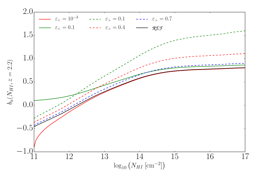
Figure 9: Column density dependence of our simple bias model at $z=2.2$ for different values of $(\varepsilon_{<},\varepsilon_{>})$. The black lines show the Reference Model of $(\varepsilon_{<},\varepsilon_{>})=(0.01,0.9)$ and $\sigma_{f}=1.68$. The array of solid colored lines vary $\varepsilon_{<}$ from the refernece; the array of dashed colored lines vary $\varepsilon_{>}$.

Figure  9 shows the effect of varying the parameters $(\varepsilon_{<},\varepsilon_{>})$ on $b(N_{\rm HI})$. Observations suggest that for DLAs, i.e. $N_{\rm HI}>10^{20.3}$cm^-2, $b(N_{\rm HI})\approx 2$ [98, 99], so the bias values should be below this threshold at the lower $N_{\rm HI}$ we consider. The exact values of the $(\varepsilon_{<},\varepsilon_{>})$ parameters for the Reference Model were fixed such that the low-$k$ power spectrum agrees with that of the mocks. The values required for $(\varepsilon_{<},\varepsilon_{>})$ in the Reference Model as well as the other cases shown in Figure  9 are consistent with the range we physically motivate, except $\varepsilon_{>}=0.1$ which is outside this range. Especially if we exclude this $\varepsilon_{>}=0.1$ curve, the range of bias values of the different models is relatively small. It would be interesting to compare the bias values in this model to full numerical simulations

References

- [1] P. McDonald, J. Miralda-Escudé, M. Rauch, W. L. W. Sargent, T. A. Barlow, R. Cen, and J. P. Ostriker, The Observed Probability Distribution Function, Power Spectrum, and Correlation Function of the Transmitted Flux in the Ly Forest, ApJ 543 (Nov., 2000) 1–23, [astro-ph/9911196].
- [2] M. Zaldarriaga, U. Seljak, and L. Hui, Correlations in the Ly Forest: Testing the Gravitational Instability Paradigm, ApJ 551 (Apr., 2001) 48–56, [astro-ph/0].
- [3] R. A. C. Croft, D. H. Weinberg, M. Bolte, S. Burles, L. Hernquist, N. Katz, D. Kirkman, and D. Tytler, Toward a Precise Measurement of Matter Clustering: Ly Forest Data at Redshifts 2-4, ApJ 581 (Dec., 2002) 20–52, [astro-ph/0012324].
- [4] M. Zaldarriaga, R. Scoccimarro, and L. Hui, Inferring the Linear Power Spectrum from the Ly Forest, ApJ 590 (June, 2003) 1–7, [astro-ph/0].
- [5] U. Seljak, P. McDonald, and A. Makarov, Cosmological constraints from the cosmic microwave background and Lyman forest revisited, MNRAS 342 (July, 2003) L79–L84, [astro-ph/0].
- [6] P. McDonald, Toward a Measurement of the Cosmological Geometry at z ~ 2: Predicting Ly Forest Correlation in Three Dimensions and the Potential of Future Data Sets, ApJ 585 (Mar., 2003) 34–51, [astro-ph/0108064].
- [7] M. Viel, M. G. Haehnelt, and V. Springel, Inferring the dark matter power spectrum from the Lyman forest in high-resolution QSO absorption spectra, MNRAS 354 (Nov., 2004) 684–694, [astro-ph/0404600].
- [8] M. Viel, S. Matarrese, A. Heavens, M. G. Haehnelt, T.-S. Kim, V. Springel, and L. Hernquist, The bispectrum of the Lyman forest at z~ 2-2.4 from a large sample of UVES QSO absorption spectra (LUQAS), MNRAS 347 (Jan., 2004) L26–L30, [astro-ph/0308151].
- [9] M. Viel, J. Weller, and M. G. Haehnelt, Constraints on the primordial power spectrum from high-resolution Lyman forest spectra and WMAP, MNRAS 355 (Dec., 2004) L23–L28, [astro-ph/0].
- [10] P. McDonald, U. Seljak, R. Cen, D. Shih, D. H. Weinberg, S. Burles, D. P. Schneider, D. J. Schlegel, N. A. Bahcall, J. W. Briggs, J. Brinkmann, M. Fukugita, Ž. Ivezić, S. Kent, and D. E. Vanden Berk, The Linear Theory Power Spectrum from the Ly Forest in the Sloan Digital Sky Survey, ApJ 635 (Dec., 2005) 761–783, [astro-ph/0407377].
- [11] P. McDonald, U. Seljak, S. Burles, D. J. Schlegel, D. H. Weinberg, R. Cen, D. Shih, J. Schaye, D. P. Schneider, N. A. Bahcall, J. W. Briggs, J. Brinkmann, R. J. Brunner, M. Fukugita, J. E. Gunn, Ž. Ivezić, S. Kent, R. H. Lupton, and D. E. Vanden Berk, The Ly Forest Power Spectrum from the Sloan Digital Sky Survey, ApJS 163 (Mar., 2006) 80–109, [astro-ph/0405013].
- [12] U. Seljak, A. Slosar, and P. McDonald, Cosmological parameters from combining the Lyman- forest with CMB, galaxy clustering and SN constraints, JCAP 10 (Oct., 2006) 14, [astro-ph/0604335].
- [13] A. Slosar, A. Font-Ribera, M. M. Pieri, J. Rich, J.-M. Le Goff, É. Aubourg, J. Brinkmann, N. Busca, B. Carithers, R. Charlassier, M. Cortês, R. Croft, K. S. Dawson, D. Eisenstein, J.-C. Hamilton, S. Ho, K.-G. Lee, R. Lupton, P. McDonald, B. Medolin, D. Muna, J. Miralda-Escudé, A. D. Myers, R. C. Nichol, N. Palanque-Delabrouille, I. Pâris, P. Petitjean, Y. Piškur, E. Rollinde, N. P. Ross, D. J. Schlegel, D. P. Schneider, E. Sheldon, B. A. Weaver, D. H. Weinberg, C. Yeche, and D. G. York, The Lyman- forest in three dimensions: measurements of large scale flux correlations from BOSS 1st-year data, JCAP 9 (Sept., 2011) 1, [arXiv:1104.5244].
- [14] N. G. Busca, T. Delubac, J. Rich, S. Bailey, A. Font-Ribera, D. Kirkby, J.-M. Le Goff, M. M. Pieri, A. Slosar, É. Aubourg, J. E. Bautista, D. Bizyaev, M. Blomqvist, A. S. Bolton, J. Bovy, H. Brewington, A. Borde, J. Brinkmann, B. Carithers, R. A. C. Croft, K. S. Dawson, G. Ebelke, D. J. Eisenstein, J.-C. Hamilton, S. Ho, D. W. Hogg, K. Honscheid, K.-G. Lee, B. Lundgren, E. Malanushenko, V. Malanushenko, D. Margala, C. Maraston, K. Mehta, J. Miralda-Escudé, A. D. Myers, R. C. Nichol, P. Noterdaeme, M. D. Olmstead, D. Oravetz, N. Palanque-Delabrouille, K. Pan, I. Pâris, W. J. Percival, P. Petitjean, N. A. Roe, E. Rollinde, N. P. Ross, G. Rossi, D. J. Schlegel, D. P. Schneider, A. Shelden, E. S. Sheldon, A. Simmons, S. Snedden, J. L. Tinker, M. Viel, B. A. Weaver, D. H. Weinberg, M. White, C. Yèche, and D. G. York, Baryon acoustic oscillations in the Ly forest of BOSS quasars, A&A 552 (Apr., 2013) A96, [arXiv:1211.2616].
- [15] A. Slosar, V. Iršič, D. Kirkby, S. Bailey, N. G. Busca, T. Delubac, J. Rich, É. Aubourg, J. E. Bautista, V. Bhardwaj, M. Blomqvist, A. S. Bolton, J. Bovy, J. Brownstein, B. Carithers, R. A. C. Croft, K. S. Dawson, A. Font-Ribera, J.-M. Le Goff, S. Ho, K. Honscheid, K.-G. Lee, D. Margala, P. McDonald, B. Medolin, J. Miralda-Escudé, A. D. Myers, R. C. Nichol, P. Noterdaeme, N. Palanque-Delabrouille, I. Pâris, P. Petitjean, M. M. Pieri, Y. Piškur, N. A. Roe, N. P. Ross, G. Rossi, D. J. Schlegel, D. P. Schneider, N. Suzuki, E. S. Sheldon, U. Seljak, M. Viel, D. H. Weinberg, and C. Yèche, Measurement of baryon acoustic oscillations in the Lyman- forest fluctuations in BOSS data release 9, JCAP 4 (Apr., 2013) 26, [arXiv:1301.3459].
- [16] N. Palanque-Delabrouille, C. Yèche, A. Borde, J.-M. Le Goff, G. Rossi, M. Viel, É. Aubourg, S. Bailey, J. Bautista, M. Blomqvist, A. Bolton, J. S. Bolton, N. G. Busca, B. Carithers, R. A. C. Croft, K. S. Dawson, T. Delubac, A. Font-Ribera, S. Ho, D. Kirkby, K.-G. Lee, D. Margala, J. Miralda-Escudé, D. Muna, A. D. Myers, P. Noterdaeme, I. Pâris, P. Petitjean, M. M. Pieri, J. Rich, E. Rollinde, N. P. Ross, D. J. Schlegel, D. P. Schneider, A. Slosar, and D. H. Weinberg, The one-dimensional Ly forest power spectrum from BOSS, A&A 559 (Nov., 2013) A85, [arXiv:1306.5896].
- [17] N. Palanque-Delabrouille, C. Yèche, J. Baur, C. Magneville, G. Rossi, J. Lesgourgues, A. Borde, E. Burtin, J.-M. LeGoff, J. Rich, M. Viel, and D. Weinberg, Neutrino masses and cosmology with Lyman-alpha forest power spectrum, JCAP 11 (Nov., 2015) 011, [arXiv:1506.05976].
- [18] J. E. Bautista, S. Bailey, A. Font-Ribera, M. M. Pieri, N. G. Busca, J. Miralda-Escudé, N. Palanque-Delabrouille, J. Rich, K. Dawson, Y. Feng, J. Ge, S. G. A. Gontcho, S. Ho, J. M. Le Goff, P. Noterdaeme, I. Pâris, G. Rossi, and D. Schlegel, Mock Quasar-Lyman- forest data-sets for the SDSS-III Baryon Oscillation Spectroscopic Survey, JCAP 5 (May, 2015) 060, [arXiv:1412.0658].
- [19] J. Baur, N. Palanque-Delabrouille, C. Yèche, A. Boyarsky, O. Ruchayskiy, É. Armengaud, and J. Lesgourgues, Constraints from Ly- forests on non-thermal dark matter including resonantly-produced sterile neutrinos, ArXiv e-prints (June, 2017) [arXiv:1706.03118].
- [20] J. E. Bautista, N. G. Busca, J. Guy, J. Rich, M. Blomqvist, H. du Mas des Bourboux, M. M. Pieri, A. Font-Ribera, S. Bailey, T. Delubac, D. Kirkby, J.-M. Le Goff, D. Margala, A. Slosar, J. A. Vazquez, J. R. Brownstein, K. S. Dawson, D. J. Eisenstein, J. Miralda-Escudé, P. Noterdaeme, N. Palanque-Delabrouille, I. Pâris, P. Petitjean, N. P. Ross, D. P. Schneider, D. H. Weinberg, and C. Yèche, Measurement of baryon acoustic oscillation correlations at z = 2.3 with SDSS DR12 Ly-Forests, A&A 603 (June, 2017) A12, [arXiv:1702.00176].
- [21] H. du Mas des Bourboux, J.-M. Le Goff, M. Blomqvist, N. G. Busca, J. Guy, J. Rich, C. Yèche, J. E. Bautista, É. Burtin, K. S. Dawson, D. J. Eisenstein, A. Font-Ribera, D. Kirkby, J. Miralda-Escudé, P. Noterdaeme, I. Pâris, P. Petitjean, I. Pérez-Ràfols, M. M. Pieri, N. P. Ross, D. J. Schlegel, D. P. Schneider, A. Slosar, D. H. Weinberg, and P. Zarrouk, Baryon acoustic oscillations from the complete SDSS-III Ly-quasar cross-correlation function at , ArXiv e-prints (Aug., 2017) [arXiv:1708.02225].
- [22] J. Schaye, T. Theuns, M. Rauch, G. Efstathiou, and W. L. W. Sargent, The thermal history of the intergalactic medium∗, MNRAS 318 (Nov., 2000) 817–826, [astro-ph/9912432].
- [23] M. Ricotti, N. Y. Gnedin, and J. M. Shull, The Evolution of the Effective Equation of State of the Intergalactic Medium, ApJ 534 (May, 2000) 41–56, [astro-ph/9906413].
- [24] T. Theuns and S. Zaroubi, A wavelet analysis of the spectra of quasi-stellar objects, MNRAS 317 (Oct., 2000) 989–995, [astro-ph/0002172].
- [25] M. Viel and M. G. Haehnelt, Cosmological and astrophysical parameters from the Sloan Digital Sky Survey flux power spectrum and hydrodynamical simulations of the Lyman forest, MNRAS 365 (Jan., 2006) 231–244, [astro-ph/0508177].
- [26] T. Theuns, S. Zaroubi, T.-S. Kim, P. Tzanavaris, and R. F. Carswell, Temperature fluctuations in the intergalactic medium, MNRAS 332 (May, 2002) 367–382, [astro-ph/0110600].
- [27] J. S. Bolton, M. Viel, T.-S. Kim, M. G. Haehnelt, and R. F. Carswell, Possible evidence for an inverted temperature-density relation in the intergalactic medium from the flux distribution of the Ly forest, MNRAS 386 (May, 2008) 1131–1144, [arXiv:0711.2064].
- [28] A. Lidz, C.-A. Faucher-Giguère, A. Dall’Aglio, M. McQuinn, C. Fechner, M. Zaldarriaga, L. Hernquist, and S. Dutta, A Measurement of Small-scale Structure in the 2.2-4.2 Ly Forest, ApJ 718 (July, 2010) 199–230, [arXiv:0909.5210].
- [29] J. S. Bolton, G. D. Becker, J. S. B. Wyithe, M. G. Haehnelt, and W. L. W. Sargent, A first direct measurement of the intergalactic medium temperature around a quasar at z = 6, MNRAS 406 (July, 2010) 612–625, [arXiv:1001.3415].
- [30] G. D. Becker, J. S. Bolton, M. G. Haehnelt, and W. L. W. Sargent, Detection of extended He II reionization in the temperature evolution of the intergalactic medium, MNRAS 410 (Jan., 2011) 1096–1112, [arXiv:1008.2622].
- [31] A. Garzilli, J. S. Bolton, T.-S. Kim, S. Leach, and M. Viel, The intergalactic medium thermal history at redshift z = 1.7-3.2 from the Ly forest: a comparison of measurements using wavelets and the flux distribution, MNRAS 424 (Aug., 2012) 1723–1736, [arXiv:1202.3577].
- [32] G. C. Rudie, C. C. Steidel, and M. Pettini, The Temperature-Density Relation in the Intergalactic Medium at Redshift langzrang = 2.4, ApJL 757 (Oct., 2012) L30, [arXiv:1209.0005].
- [33] K.-G. Lee, J. P. Hennawi, D. N. Spergel, D. H. Weinberg, D. W. Hogg, M. Viel, J. S. Bolton, S. Bailey, M. M. Pieri, W. Carithers, D. J. Schlegel, B. Lundgren, N. Palanque-Delabrouille, N. Suzuki, D. P. Schneider, and C. Yeche, IGM Constraints from the SDSS-III/BOSS DR9 Ly-alpha Forest Flux Probability Distribution Function, ArXiv e-prints (May, 2014) [arXiv:1405.1072].
- [34] E. Boera, M. T. Murphy, G. D. Becker, and J. S. Bolton, The thermal history of the intergalactic medium down to redshift z = 1.5: a new curvature measurement, MNRAS 441 (July, 2014) 1916–1933, [arXiv:1404.1083].
- [35] J. S. Bolton, G. D. Becker, M. G. Haehnelt, and M. Viel, A consistent determination of the temperature of the intergalactic medium at redshift z = 2.4, MNRAS 438 (Mar., 2014) 2499–2507, [arXiv:1308.4411].
- [36] A. Rorai, J. F. Hennawi, J. Oñorbe, M. White, J. X. Prochaska, G. Kulkarni, M. Walther, Z. Lukić, and K.-G. Lee, Measurement of the small-scale structure of the intergalactic medium using close quasar pairs, Science 356 (Apr., 2017) 418–422, [arXiv:1704.08366].
- [37] H. Hiss, M. Walther, J. F. Hennawi, J. Oñorbe, J. M. O’Meara, and A. Rorai, A New Measurement of the Temperature Density Relation of the IGM From Voigt Profile Fitting, ArXiv e-prints (Oct., 2017) [arXiv:1710.00700].
- [38] V. K. Narayanan, D. N. Spergel, R. Davé, and C.-P. Ma, Constraints on the Mass of Warm Dark Matter Particles and the Shape of the Linear Power Spectrum fro m the Ly Forest, ApJL 543 (Nov., 2000) L103–L106, [astro-ph/0005095].
- [39] M. Viel, J. Lesgourgues, M. G. Haehnelt, S. Matarrese, and A. Riotto, Constraining warm dark matter candidates including sterile neutrinos and light gravitinos with WMAP and the Lyman- forest, Phys. Rev. D 71 (Mar., 2005) 063534, [astro-ph/0501562].
- [40] U. Seljak, A. Makarov, P. McDonald, and H. Trac, Can Sterile Neutrinos Be the Dark Matter?, Physical Review Letters 97 (Nov., 2006) 191303, [astro-ph/0602430].
- [41] M. Viel, G. D. Becker, J. S. Bolton, M. G. Haehnelt, M. Rauch, and W. L. W. Sargent, How Cold Is Cold Dark Matter? Small-Scales Constraints from the Flux Power Spectrum of the High-Redshift Lyman- Forest, Physical Review Letters 100 (Feb., 2008) 041304, [arXiv:0709.0131].
- [42] S. Bird, H. V. Peiris, M. Viel, and L. Verde, Minimally parametric power spectrum reconstruction from the Lyman forest, MNRAS 413 (May, 2011) 1717–1728, [arXiv:1010.1519].
- [43] M. Viel, G. D. Becker, J. S. Bolton, and M. G. Haehnelt, Warm dark matter as a solution to the small scale crisis: New constraints from high redshift Lyman- forest data, Phys. Rev. D 88 (Aug., 2013) 043502, [arXiv:1306.2314].
- [44] J. Baur, N. Palanque-Delabrouille, C. Yèche, C. Magneville, and M. Viel, Lyman-alpha forests cool warm dark matter, JCAP 8 (Aug., 2016) 012, [arXiv:1512.01981].
- [45] C. Yeche, N. Palanque-Delabrouille, J. . Baur, and H. du Mas des BourBoux, Constraints on neutrino masses from Lyman-alpha forest power spectrum with BOSS and XQ-100, ArXiv e-prints (Feb., 2017) [arXiv:1702.03314].
- [46] V. Iršič, M. Viel, M. G. Haehnelt, J. S. Bolton, and G. D. Becker, First Constraints on Fuzzy Dark Matter from Lyman- Forest Data and Hydrodynamical Simulations, Physical Review Letters 119 (July, 2017) 031302, [arXiv:1703.04683].
- [47] V. Iršič, M. Viel, M. G. Haehnelt, J. S. Bolton, S. Cristiani, G. D. Becker, V. D’Odorico, G. Cupani, T.-S. Kim, T. A. M. Berg, S. López, S. Ellison, L. Christensen, K. D. Denney, and G. Worseck, New constraints on the free-streaming of warm dark matter from intermediate and small scale Lyman- forest data, Phys. Rev. D 96 (July, 2017) 023522, [arXiv:1702.01764].
- [48] E. Armengaud, N. Palanque-Delabrouille, C. Yèche, D. J. E. Marsh, and J. Baur, Constraining the mass of light bosonic dark matter using SDSS Lyman- forest, ArXiv e-prints (Mar., 2017) [arXiv:1703.09126].
- [49] J. S. Bolton, E. Puchwein, D. Sijacki, M. G. Haehnelt, T.-S. Kim, A. Meiksin, J. A. Regan, and M. Viel, The Sherwood simulation suite: overview and data comparisons with the Lyman-alpha forest at redshifts , ArXiv e-prints (May, 2016) [arXiv:1605.03462].
- [50] C.-P. Ma and J. N. Fry, Deriving the Nonlinear Cosmological Power Spectrum and Bispectrum from Analytic Dark Matter Halo Profiles and Mass Functions, ApJ 543 (Nov., 2000) 503–513, [astro-ph/0003343].
- [51] U. Seljak, Analytic model for galaxy and dark matter clustering, MNRAS 318 (Oct., 2000) 203–213, [astro-ph/0001493].
- [52] A. Cooray and R. Sheth, Halo models of large scale structure, Phys. Rep. 372 (Dec., 2002) 1–129, [astro-ph/0206508].
- [53] U. Seljak, N. Hamaus, and V. Desjacques, How to Suppress the Shot Noise in Galaxy Surveys, Physical Review Letters 103 (Aug., 2009) 091303, [arXiv:0904.2963].
- [54] A. J. Mead, J. A. Peacock, C. Heymans, S. Joudaki, and A. F. Heavens, An accurate halo model for fitting non-linear cosmological power spectra and baryonic feedback models, MNRAS 454 (Dec., 2015) 1958–1975, [arXiv:1505.07833].
- [55] T. Baldauf, U. Seljak, R. E. Smith, N. Hamaus, and V. Desjacques, Halo stochasticity from exclusion and nonlinear clustering, Phys. Rev. D 88 (Oct., 2013) 083507, [arXiv:1305.2917].
- [56] D. Ginzburg, V. Desjacques, and K. C. Chan, Shot noise and biased tracers: A new look at the halo model, Phys. Rev. D 96 (Oct., 2017) 083528, [arXiv:1706.08738].
- [57] A. A. Meiksin, The physics of the intergalactic medium, Reviews of Modern Physics 81 (Oct., 2009) 1405–1469, [arXiv:0711.3358].
- [58] M. McQuinn, The Evolution of the Intergalactic Medium, ArXiv e-prints (Nov., 2015) [arXiv:1512.00086].
- [59] J. Miralda-Escudé, R. Cen, J. P. Ostriker, and M. Rauch, The Ly alpha Forest from Gravitational Collapse in the Cold Dark Matter + Lambda Model, ApJ 471 (Nov., 1996) 582, [astro-ph/9511013].
- [60] L. Hernquist, N. Katz, D. H. Weinberg, and J. Miralda-Escudé, The Lyman-Alpha Forest in the Cold Dark Matter Model, ApJL 457 (Feb., 1996) L51, [astro-ph/9509105].
- [61] J. X. Prochaska, J. M. O’Meara, and G. Worseck, A Definitive Survey for Lyman Limit Systems at z ~ 3.5 with the Sloan Digital Sky Survey, ApJ 718 (July, 2010) 392–416, [arXiv:0912.0292].
- [62] P. Noterdaeme, P. Petitjean, W. C. Carithers, I. Pâris, A. Font-Ribera, S. Bailey, E. Aubourg, D. Bizyaev, G. Ebelke, H. Finley, J. Ge, E. Malanushenko, V. Malanushenko, J. Miralda-Escudé, A. D. Myers, D. Oravetz, K. Pan, M. M. Pieri, N. P. Ross, D. P. Schneider, A. Simmons, and D. G. York, Column density distribution and cosmological mass density of neutral gas: Sloan Digital Sky Survey-III Data Release 9, A&A 547 (Nov., 2012) L1, [arXiv:1210.1213].
- [63] J. Schaye, Model-independent Insights into the Nature of the Ly Forest and the Distribution of Matter in the Universe, ApJ 559 (Oct., 2001) 507–515, [astro-ph/0104272].
- [64] M. J. Rees, Lyman absorption lines in quasar spectra - Evidence for gravitationally-confined gas in dark minihaloes, MNRAS 218 (Jan., 1986) 25P–30P.
- [65] H. Bi and A. F. Davidsen, Evolution of Structure in the Intergalactic Medium and the Nature of the Ly Forest, ApJ 479 (Apr., 1997) 523–542, [astro-ph/9611062].
- [66] A. Font-Ribera, P. McDonald, and J. Miralda-Escudé, Generating mock data sets for large-scale Lyman- forest correlation measurements, JCAP 1 (Jan., 2012) 1, [arXiv:1108.5606].
- [67] W. H. Press, G. B. Rybicki, and D. P. Schneider, Properties of high-redshift Lyman-alpha clouds. I - Statistical analysis of the Schneider-Schmidt-Gunn quasars, ApJ 414 (Sept., 1993) 64–81, [astro-ph/9303016].
- [68] L. Zuo and J. R. Bond, The transmission correlation in the QSO Ly(alpha) forest produced by finite width lines, ApJ 423 (Mar., 1994) 73–93.
- [69] J. Liske, J. K. Webb, and R. F. Carswell, Large-scale structure in the Lyman-alpha forest: a new technique, MNRAS 301 (Dec., 1998) 787–796, [astro-ph/9808082].
- [70] N. Kaiser, Clustering in real space and in redshift space, MNRAS 227 (July, 1987) 1–21.
- [71] A. Arinyo-i-Prats, J. Miralda-Escudé, M. Viel, and R. Cen, The non-linear power spectrum of the Lyman alpha forest, JCAP 12 (Dec., 2015) 017, [arXiv:1506.04519].
- [72] U. Seljak, Bias, redshift space distortions and primordial nongaussianity of nonlinear transformations: application to Ly- forest, JCAP 3 (Mar., 2012) 4, [arXiv:1201.0594].
- [73] A. M. Cieplak and A. Slosar, Towards physics responsible for large-scale Lyman- forest bias parameters, JCAP 3 (Mar., 2016) 016, [arXiv:1509.07875].
- [74] T.-S. Kim, M. Viel, M. G. Haehnelt, R. F. Carswell, and S. Cristiani, The power spectrum of the flux distribution in the Lyman forest of a large sample of UVES QSO absorption spectra (LUQAS), MNRAS 347 (Jan., 2004) 355–366, [astro-ph/0308103].
- [75] B. Carswell et al.: http://www.ast.cam.ac.uk/rfc/vpfit.html.
- [76] M. Viel, M. G. Haehnelt, R. F. Carswell, and T.-S. Kim, The effect of (strong) discrete absorption systems on the Lyman forest flux power spectrum, MNRAS 349 (Apr., 2004) L33–L37, [astro-ph/0308078].
- [77] A. Font-Ribera and J. Miralda-Escudé, The effect of high column density systems on the measurement of the Lyman- forest correlation function, JCAP 7 (July, 2012) 28, [arXiv:1205.2018].
- [78] P. McDonald, U. Seljak, R. Cen, P. Bode, and J. P. Ostriker, Physical effects on the Ly forest flux power spectrum: damping wings, ionizing radiation fluctuations and galactic winds, MNRAS 360 (July, 2005) 1471–1482, [astro-ph/0407378].
- [79] M. McQuinn and M. White, On estimating Ly forest correlations between multiple sightlines, MNRAS 415 (Aug., 2011) 2257–2269, [arXiv:1102.1752].
- [80] K. K. Rogers, S. Bird, H. V. Peiris, A. Pontzen, A. Font-Ribera, and B. Leistedt, Simulating the effect of high column density absorbers on the one-dimensional Lyman-alpha forest flux power spectrum, ArXiv e-prints (June, 2017) [arXiv:1706.08532].
- [81] A. Garzilli, T. Theuns, and J. Schaye, The broadening of Lyman- forest absorption lines, MNRAS 450 (June, 2015) 1465–1476, [arXiv:1502.05715].
- [82] M. McQuinn, S. P. Oh, and C.-A. Faucher-Giguère, On Lyman-limit Systems and the Evolution of the Intergalactic Ionizing Background, ApJ 743 (Dec., 2011) 82, [arXiv:1101.1964].
- [83] G. Altay, T. Theuns, J. Schaye, N. H. M. Crighton, and C. Dalla Vecchia, Through Thick and Thin – H I Absorption in Cosmological Simulations, ApJL 737 (Aug., 2011) L37, [arXiv:1012.4014].
- [84] L. Hui and N. Y. Gnedin, Equation of state of the photoionized intergalactic medium, MNRAS 292 (Nov., 1997) 27, [astro-ph/9612232].
- [85] M. McQuinn and P. R. Upton Sanderbeck, On the intergalactic temperature-density relation, MNRAS 456 (Feb., 2016) 47–54, [arXiv:1505.07875].
- [86] R. Cen and J. P. Ostriker, Where Are the Baryons? II. Feedback Effects, ApJ 650 (Oct., 2006) 560–572, [astro-ph/0601008].
- [87] N. Y. Gnedin and L. Hui, Probing the universe with the Lyman alpha forest: 1. Hydrodynamics of the low density IGM, Mon. Not. Roy. Astron. Soc. 296 (1998) 44–55, [astro-ph/9706219].
- [88] G. Kulkarni, J. F. Hennawi, J. Oñorbe, A. Rorai, and V. Springel, Characterizing the Pressure Smoothing Scale of the Intergalactic Medium, ApJ 812 (Oct., 2015) 30, [arXiv:1504.00366].
- [89] Y. Noh and M. McQuinn, A physical understanding of how reionization suppresses accretion on to dwarf haloes, MNRAS 444 (Oct., 2014) 503–514, [arXiv:1401.0737].
- [90] K. Lai, A. Lidz, L. Hernquist, and M. Zaldarriaga, The Impact of Temperature Fluctuations on the Ly Forest Power Spectrum, ApJ 644 (June, 2006) 61–70, [astro-ph/0510841].
- [91] J. R. Bond, S. Cole, G. Efstathiou, and N. Kaiser, Excursion set mass functions for hierarchical Gaussian fluctuations, ApJ 379 (Oct., 1991) 440–460.
- [92] J. F. Navarro, C. S. Frenk, and S. D. M. White, The Structure of Cold Dark Matter Halos, ApJ 462 (May, 1996) 563, [astro-ph/9508025].
- [93] V. Desjacques, D. Jeong, and F. Schmidt, Tidal shear and the consistency of microscopic Lagrangian halo approaches, ArXiv e-prints (Nov., 2017) [arXiv:1711.06745].
- [94] J. Schaye, A. Aguirre, T.-S. Kim, T. Theuns, M. Rauch, and W. L. W. Sargent, Metallicity of the Intergalactic Medium Using Pixel Statistics. II. The Distribution of Metals as Traced by C IV, ApJ 596 (Oct., 2003) 768–796, [astro-ph/0306469].
- [95] A. Aguirre, J. Schaye, T.-S. Kim, T. Theuns, M. Rauch, and W. L. W. Sargent, Metallicity of the Intergalactic Medium Using Pixel Statistics. III. Silicon, ApJ 602 (Feb., 2004) 38–50, [astro-ph/0310664].
- [96] A. Aguirre, C. Dow-Hygelund, J. Schaye, and T. Theuns, Metallicity of the Intergalactic Medium Using Pixel Statistics. IV. Oxygen, ApJ 689 (Dec., 2008) 851–864, [arXiv:0712.1239].
- [97] A. Garzilli, A. Boyarsky, and O. Ruchayskiy, Cutoff in the Lyman alpha forest power spectrum: warm IGM or warm dark matter?, ArXiv e-prints (Oct., 2015) [arXiv:1510.07006].
- [98] A. Font-Ribera, J. Miralda-Escudé, E. Arnau, B. Carithers, K.-G. Lee, P. Noterdaeme, I. Pâris, P. Petitjean, J. Rich, E. Rollinde, N. P. Ross, D. P. Schneider, M. White, and D. G. York, The large-scale cross-correlation of Damped Lyman alpha systems with the Lyman alpha forest: first measurements from BOSS, JCAP 11 (Nov., 2012) 059, [arXiv:1209.4596].
- [99] I. Pérez-Ràfols, A. Font-Ribera, J. Miralda-Escudé, M. Blomqvist, S. Bird, N. Busca, H. du Mas des Bourboux, L. Mas-Ribas, P. Noterdaeme, P. Petitjean, J. Rich, and D. P. Schneider, The SDSS-DR12 large-scale cross-correlation of damped Lyman alpha systems with the Lyman alpha forest, MNRAS 473 (Jan., 2018) 3019–3038, [arXiv:1709.00889].