Spitzer Matching survey of the UltraVISTA ultra-deep Stripes (SMUVS):
Full-mission IRAC Mosaics and Catalogs

Abstract

This paper describes new deep 3.6 and 4.5 $\mu$m imaging of three UltraVISTA near-infrared survey stripes within the COSMOS field. The observations were carried out with Spitzer’s Infrared Array Camera (IRAC) for the Spitzer Matching Survey of the Ultra-VISTA Deep Stripes (SMUVS). In this work we present our data reduction techniques, and document the resulting mosaics, coverage maps, and catalogs in both IRAC passbands for the three easternmost UltraVISTA survey stripes, covering a combined area of about 0.66 deg², of which 0.45 deg² have at least 20 hr integration time. SMUVS reaches point-source sensitivities of about 25.0 AB mag (0.13 $\mu$Jy) at both 3.6 and 4.5 $\mu$m with a significance of 4$\sigma$, accounting for both survey sensitivity and source confusion. To this limit the SMUVS catalogs contain a total of $\sim$350,000 sources, each of which is detected significantly in at least one IRAC band. Because of its uniform and high sensitivity, relatively large area coverage, and the wide array of ancillary data available in COSMOS, the SMUVS survey will be useful for a large number of cosmological investigations. We make all images and catalogues described herein publicly available via the Spitzer Science Center.

1 Introduction

Measurements of galaxy number density and stellar-mass evolution at high redshifts ($z>3$) are the foundation for a proper understanding of how galaxy buildup proceeded in the early Universe. Number density and stellar mass estimates directly constrain models of the candidate mechanisms for galaxy growth, such as galaxy mergers (e.g., Hopkins et al. 2006; Somerville et al. 2008) or cold gas accretion within gas-rich proto-disks (e.g., Dekel et al. 2009). Whatever the mechanisms might be that govern galaxy evolution, they must reproduce the observed distribution of baryons at high redshift, and connect it to the subsequent evolution of galaxies within dark matter haloes.

For galaxies out to redshifts $z=2-3$, stellar masses are typically derived from broadband photometry between the (rest-frame) 4000Å break and $K$-band (e.g., Bell & de Jong 2001), because observations in this interval are more sensitive to the light from the stellar populations that dominate the stellar mass. Beyond $z=3$, however, it becomes very challenging to photometer the stellar populations that dominate the total stellar mass because of the high sky backgrounds at wavelengths longward of $K$. For galaxies at $z>3$, one must therefore turn to mid-infrared observations from space. This is exactly why $3.6-4.5$ $\mu$m imaging with the Infrared Array Camera (IRAC; Fazio et al. 2004) aboard the Spitzer Space Telescope (Werner et al. 2004) is indispensable for mapping the rest-frame near-IR light from distant galaxies. IRAC observations are also necessary to identify distant active galactic nuclei (AGN), particularly when the nuclear activity is too obscured by dust to be detected in X rays (e.g., Lacy et al. 2004; Stern et al. 2005; Caputi 2013, 2014).

Recent studies of massive galaxies ($M>\sim 10^{11}M_{\sun}$) at high redshifts have revealed significant number-density evolution between $z=5$ and $z=3$, consistent with much faster assembly than between $z=2$ and $z=0$ (Caputi et al. 2011; Ilbert et al. 2013; Muzzin et al. 2013; Stefanon et al. 2015). By contrast, relatively little is known about the evolution of intermediate-mass galaxies ($M\sim 10^{10}M_{\sun}$) at $z>3$, because typical IRAC surveys are too shallow to yield complete samples of these galaxies over large areas of the sky. This is unfortunate, because the relatively numerous intermediate-mass galaxies are expected to contain most of the stellar mass of the Universe at high redshifts (e.g., Caputi et al. 2015). Identifying and characterizing complete samples of intermediate-mass galaxies is therefore crucial for constraining galaxy formation models.

Optically selected galaxy samples at $z>3$ have yielded some important information about intermediate-mass galaxies, such as typical Lyman-break galaxies (e.g., Steidel et al. 2003; Malhotra et al. 2005; Shapley et al. 2006). However, these samples are not fully representative of intermediate-mass galaxies at high redshifts because they are biased against dust-obscured sources, and the stellar-mass estimates of high-redshift Lyman-break galaxies are robust only when IRAC photometry is available. To obtain galaxy samples that are complete in stellar mass at high redshifts, it is necessary to avoid dust attenuation by selecting targets in deep infrared maps, and it helps greatly to have coextensive Spitzer/IRAC imaging (e.g., Caputi et al. 2014) in order to get multiple measurements of the redshifted stellar continua.

In this contribution, we describe a new IRAC survey designed to provide deep rest-frame optical/near-IR imaging over a large area of the sky for which deep ground-based imaging is available. This survey, the Spitzer Matching survey of the UltraVISTA ultra-deep Stripes (SMUVS), covers three ultra-deep stripes of the UltraVISTA survey (McCracken et al. 2012) within the COSMOS field with extremely sensitive semi-continuous imaging in both operating IRAC bands. SMUVS is intended to provide the community with the best prospects to build upon present knowledge of galaxy evolution beyond $z=3$. Figure 1 illustrates the relationship of SMUVS to other extragalactic surveys carried out with Spitzer.

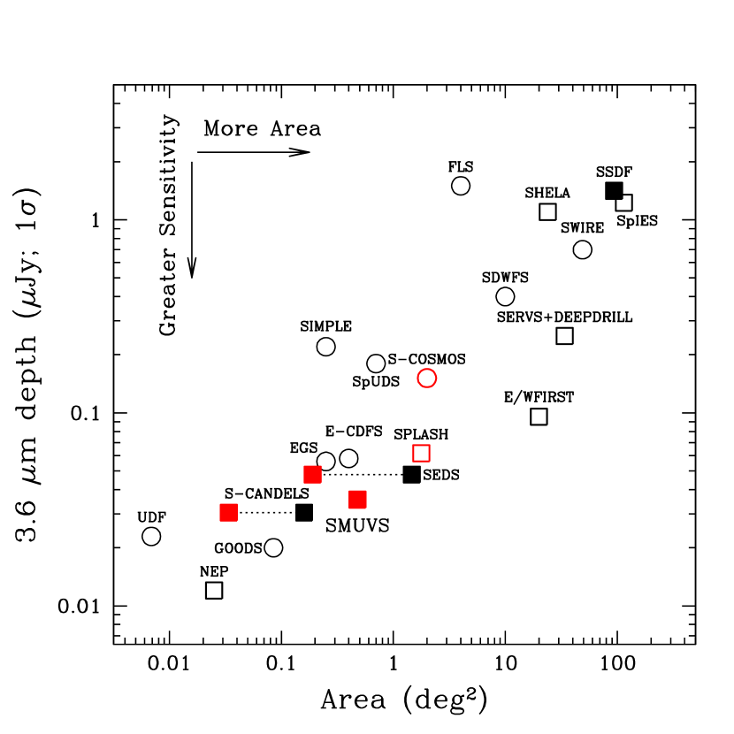
Figure 1: SMUVS in relation to other completed Spitzer/IRAC extragalactic surveys. Circles and squares indicate the 3.6 $\mu$m $1\sigma$ point-source sensitivities for surveys executed during the cryogenic and warm mission phases, respectively. Solid squares indicate sensitivities calculated with simulations; the other sensitivities shown are either taken from the literature or from the online calculator SENS-PET under low-background conditions. All red symbols indicate IRAC surveys carried out within the COSMOS field specifically, including S-COSMOS (Scoville et al. 2007), SPLASH (Steinhardt et al. 2014), SEDS (Ashby et al. 2013a), and S-CANDELS (Ashby et al. 2015), in addition to SMUVS. SEDS and S-CANDELS are multi-field surveys for which the total and the COSMOS-specific portions are indicated with connected black and red squares. Also shown are the First Look Survey (FLS; Fang et al. 2004), Spitzer-SPT Deep Field (SSDF; Ashby et al. 2013b), Spitzer-IRAC Equatorial Survey (SpIES; Timlin et al. 2016), Spitzer-HETDEX Exploratory Large-area Survey (SHELA; Papovich et al. 2016), Spitzer Wide-area Infrared Extragalactic Survey (SWIRE; Lonsdale et al. 2003, 2004), Spitzer Deep, Wide-Field Survey (SDWFS; Ashby et al. 2009), Spitzer Extragalactic Representative Volume Survey (SERVS; Mauduit et al. 2012) augmented by additional, contiguous coverage to the same depth from DEEPDRILL (M. Lacy, priv. comm.), Spitzer IRAC/MUSYC Public Legacy in E-CDFS (SIMPLE; Damen et al. 2011), Spitzer Public Legacy Survey of UKIDSS Ultra-deep Survey (SpUDS; Caputi et al. 2011), Euclid/WFIRST Spitzer Legacy Survey (E/WFIRST; PI Capak), the Extended Chandra Deep Field South (E-CDFS; Rix et al. 2004), the Extended Groth Strip (EGS; Barmby et al. 2008), the Ultra-deep Field (UDF; Labbé et al. 2013), the Great Observatories Origins Deep Survey (GOODS; Lin et al. 2012), and the IRAC dark field at the North Ecliptic Pole (NEP; Krick et al. 2009; J. Surace, priv. comm.).

This paper is organized as follows. Sec.  2 describes the UltraVISTA survey. In Secs.  3 and 4 we describe the multi-epoch IRAC observations carried out for SMUVS and other coextensive IRAC surveys, and describe how the observations were reduced to catalog form. Finally, Sec.  7 describes the tests applied to the SMUVS catalogs to validate them.

2 The UltraVISTA Ultradeep Survey within the COSMOS Field

The Cosmic Evolution Survey (COSMOS, Scoville et al. 2007) is a well-known extragalactic survey field covering $\sim 2$ deg² sited strategically at $(\alpha,\delta)=(10^{\rm h}00^{\rm m},+02^{\circ}12^{\prime})$ where it is accessible to ground-based telescopes in both the northern and southern hemispheres. In addition to high-resolution imaging with the largest contiguous HST/ACS survey so far compiled (Koekemoer et al. 2007), COSMOS benefits from extensive imaging at X-ray, optical/infrared, submillimeter, radio, and other wavelengths, plus an abundance of spectroscopy. These overlapping surveys feature a combination of high sensitivity and wide area coverage designed to sample large volumes and thereby facilitate a better understanding of galaxy evolution without undue complications from cosmic variance.

The pressing need for deep near-IR photometry within COSMOS motivated a large allocation of observing time for multiband imaging in survey mode with the VIRCAM instrument (Dalton et al. 2006) at the VISTA telescope (Emerson & Sutherland 2010). This effort is known as UltraVISTA (McCracken et al. 2012). UltraVISTA is the deepest of the public surveys being carried out with the VISTA telescope. No other near-IR survey covers as much area as deeply as UltraVISTA. Specifically, UltraVISTA has mapped $\sim 1.8$ deg² of COSMOS in $YJHK_{s}$, plus half that area in the $NB118$ narrowband filter at $1.19$ $\mu$m (Milvang-Jensen et al. 2013). UltraVISTA consists of two main parts: a deep survey reaching $K_{s}=23.7$ AB mag (5$\sigma$) over the full area, and an ultra-deep survey that will reach $K_{s}\approx 25.3$ and $H\approx 25.7$ AB mag (both 5$\sigma$) over four stripes covering a total of $\sim 0.8$ deg² in the final data release (Fig. 3; see also Fig. 1 of McCracken et al. 2012). After 8 years of observations that started at the end of 2009 the primary UltraVISTA survey is now essentially complete. The forthcoming DR4 data release will contain stacks based on re-reduced data for the first 7 years (DR3 corresponded to the first 5 years). In addition, a new UltraVISTA extension program that began in 2017 April will enlarge the area of homogeneous ultra-deep $JHK_{s}$ coverage to $\sim 1.8$ deg².

3 IRAC Mapping of the COSMOS Field

Table 1: Spitzer/IRAC Imaging Campaigns in COSMOS

PID	Epoch	Approximate TINT
		(hours)
SMUVS STRIPE 1 (10:02, +2:18)
20070	2005 Dec 30–2006 Jan 02	0.3
90042	2013 Feb 02–Mar 04	1.7
90042	2013 Jul 04–Aug 07	1.7
90042	2014 Feb 17–Mar 10	1.4
10159	2014 Jul 13–Aug 19	0.6
11016	2015 Feb 13–Mar 17	9.0
11016	2015 Jul 21–Jul 30	9.0
11016	2016 Mar 01–Mar 22	2.2
11016	2016 Aug 16–Sep 03	15.4
11016	2017 Feb 26–Apr 04	4.4
SMUVS STRIPE 2 (10:00:30, +2:14)
20070	2005 Dec 30–2006 Jan 2	0.3
61043	2010 Jan 25–Feb 04	4.0
61043	2010 Jun 10–Jun 28	4.0
61043	2011 Jan 30–Feb 06	4.0
80057	2012 Feb 04–Feb 19	36.0
80057	2012 Jun 26–Jul 09	36.0
11016	2015 Feb 24–Mar 19	9.0
11016	2015 Aug 22–Aug 27	9.0
11016	2016 Mar 02–Mar 21	6.7
11016	2016 Jul 29–Aug 19	8.3
11016	2017 Mar 02–Mar 05	1.5
SMUVS STRIPE 3 (9:59, +2:13)
20070	2005 Dec 30–2006 Jan 2	0.3
90042	2013 Feb 02–Mar 04	1.7
90042	2013 Jul 04–Aug 07	1.7
90042	2014 Feb 17–Mar 10	1.4
10159	2014 Jul 13–Aug 19	0.6
11016	2015 Feb 12–Mar 18	6.7
11016	2015 Jul 21–Aug 07	6.7
11016	2016 Mar 17–Mar 23	2.2
11016	2016 Jul 29–Aug 15	7.0
11016	2017 Mar 01–Apr 04	16.7

Note. — Spitzer/IRAC observations of the three UltraVISTA stripes covered by SMUVS. Integration times are illustrative only, due to significant variation by position within each SMUVS epoch. Coverage is not necessarily coextensive on successive epochs.

To make full use of the unprecedented depth and sensitivity of UltraVISTA’s near-IR imaging for studies of high-redshift galaxies, deep photometry at longer wavelengths is needed. Spitzer/IRAC is the obvious facility to provide it. Indeed, as described below and illustrated by Table 1, different portions of COSMOS have been observed with IRAC several times over the course of the Spitzer mission. The character of these IRAC surveys has varied considerably, and includes both wide-and-shallow and narrow-and-deep designs. Since the first visit with IRAC in Cycle 2, the Spitzer mission has spent nearly 4000 hr surveying COSMOS, much more than for any other IRAC survey completed to date. Roughly 1770 hr of Spitzer time were devoted to the new SMUVS observations described here.

3.1 IRAC Surveys of COSMOS Spanning the Last Decade

The first IRAC coverage was obtained during the cryogenic phase of the mission by Spitzer-COSMOS (S-COSMOS; Sanders et al. 2007), which imaged essentially all of COSMOS with 20 min total exposure times in all four then-operating IRAC bands. Subsequently, relatively small areas within UltraVISTA stripe 2 were imaged during Cycles 6 and 8 of Spitzer’s warm mission by the Spitzer Extended Deep Survey (SEDS; PI Fazio; Ashby et al. 2013a) and the Spitzer-Cosmic Assembly Near-Infrared Deep Extragalactic Survey (S-CANDELS; PI Fazio; Ashby et al. 2015). Then in Cycles 9 and 10, the Spitzer Large Area Survey with Hyper-Suprime-Cam (SPLASH; PI Capak; Steinhardt et al. 2014) imaged almost all of COSMOS much more deeply than S-COSMOS. The resulting combined deep coextensive IRAC and UltraVISTA imaging, with photometry spanning many wavebands (e.g., Ilbert et al. 2010; Laigle et al. 2016) proved very useful for identifying high-redshift galaxies (e.g., Steinhardt et al. 2016). However, even with SPLASH, SEDS, and S-COSMOS, the most distant galaxies remained out of reach. Thus in Cycle 11, we began a program to cover three of the UltraVISTA ultra-deep stripes to a much greater and more uniform depth with IRAC, so as to provide a much better match to the ground-based near-IR photometry, and over a wide area. This program is SMUVS: Spitzer Matching survey of the UltraVISTA ultra-deep Stripes, led by PI K. Caputi.

3.2 SMUVS Mapping Strategy

The UltraVISTA ultra-deep survey covers four parallel stripes of about 0.20 deg² each. SMUVS covered only stripes 1, 2, and 3, because they benefit from the deepest ancillary data. The observing strategy was driven by the need to integrate deeply over these three discontinuous fields – the regions with the deepest $K_{s}$ imaging – in as uniform a manner as possible, accounting for the different levels of existing coverage. For example, although S-COSMOS covered all three SMUVS stripes to a uniform depth, Stripes 1 and 3 benefit from fairly deep and uniform coverage by SPLASH. By design SPLASH did not add to the SEDS depths in Stripe 2. Much of Stripe 2, however, was covered to 12 hr depths by SEDS, a fraction of which was covered with variable but long integration times by S-CANDELS, reaching $>100$ hr in small areas. The SMUVS observations were designed to obtain deep coverage over all three stripes by filling in on top of or adjacent to the existing surveys.

Each SMUVS stripe is roughly 10′ wide in Right Ascension, and was efficiently mapped with a raster pattern having a width equal to two overlapping IRAC fields-of-view. Given constraints imposed by spacecraft scheduling needs, we mapped the stripes in the Declination direction, with small $1\times 2$ maps. We covered Stripes 1 and 3 respectively with five and six pairs of such maps (to cover the east and west sides of the stripe). Stripe 1 only needed five pointings per half stripe because a faulty chip in the VISTA-telescope camera VIRCAM prevented from collecting ultra-deep data in the southern part of the stripe. With its existing deep IRAC coverage, only two such map pairs were needed to complete Stripe 2.

Because it lies so close to the ecliptic, each year the COSMOS field is only visible to Spitzer during two short observing windows roughly 40 days long and 6 months apart, February-March and July-August. SMUVS was designed to use just the first three available visibility windows, but intense scheduling pressure delayed its completion until 2017 March. Thus SMUVS required a total of five visits to COSMOS spread out over more than two calendar years (Table 1). Since the beginning of the mission, the UltraVISTA ultra-deep stripes therefore have up to 10 distinct imaging epochs in some locations, a feature of the dataset that is useful for exploring AGN variability in the near-infrared regime (Sánchez et al. 2017).

The individual exposures were organized into self-contained segments known as Astronomical Observing Requests (AORs) roughly six hours long to accommodate the downlink schedule. Each AOR consisted of a sequence of dithered 100 s exposures obtained simultaneously in both operable IRAC detectors. All SMUVS AORs used a medium-cycling dithering pattern, which implements half-pixel subsampling to cope with cosmic rays, enforce overlap among adjacent map positions, and aid in the removal of detector artifacts. Each map position was observed with multiple AORs to accumulate the necessary integration time. To ensure high redundancy the AORs covering any map position were configured with different initial positions for the cycling dither pattern. The highly redundant dithering strategy also allowed for a thorough sampling of the PSFs.

4 Data Reduction

The SMUVS data were reduced using the same procedures that members of our team employed earlier with the SEDS and S-CANDELS datasets (Ashby et al. 2013a; 2015). The SMUVS reductions differ only in a few minor details. They are described below.

4.1 Mosaic Creation

After subtracting object-masked median-stacked sky background frames on a per-AOR basis from all SMUVS exposures to remove long-term residual images, we applied our custom column-pulldown corrector to the resulting background-subtracted frames to fix the depressed counts in individual array columns containing pixels at or near saturation. We then mosaicked the artifact-corrected exposures, grouped by IRAC band, using IRACproc (Schuster et al. 2006) within each stripe and epoch. As was done for SEDS and S-CANDELS, we mosaicked subsets of the exposures to circumvent computer memory limitations and subsequently combined these intermediate-depth mosaics into a single mosaic covering each stripe. All six SMUVS mosaics were pixellated to 0$\farcs$6 to afford slightly higher effective spatial resolution than the $\sim$1$\farcs$2 IRAC native pixel size, and were aligned to the tangent-plane projection used by the UltraVISTA collaboration (including Stripes 1 and 3, which do not contain the tangent point). All coextensive non-SMUVS exposures available in the Spitzer archive were incorporated into our mosaics after processing in the same AOR-based manner as the SMUVS data themselves. Thus our final mosaics are full-mission coadds of all IRAC exposures within each UltraVISTA stripe, including data from both the cryogenic and warm-mission phases. The resulting coverage as a function of total integration time is shown in Fig. 2.

Figure 2: Cumulative area coverage as a function of Spitzer/IRAC exposure time for SMUVS, including other, earlier observations (Table 1.) Top three panels: area versus integration time within the three UltraVISTA stripes. Bottom panel: area versus integration time for all of SMUVS, i.e., the sum of all three stripes. The data shown are derived from the full-mission IRAC mosaics, beginning with S-COSMOS (Sanders et al. 2007) during the cryogenic mission and continuing through the fifth and final SMUVS epoch in 2017 April. At 30 hr integration times, SMUVS covers about 0.3 deg², but the coverage is variable. Nonetheless SMUVS is a significant improvement in all respects over, e.g., SEDS, the COSMOS portion of which is shown in the lower panel with dotted lines.

Figures 3 and 4 show where the SMUVS coverage is located within the COSMOS field. The SMUVS mosaics and the associated coverage maps are all available from the Spitzer Exploration Science Programs website.

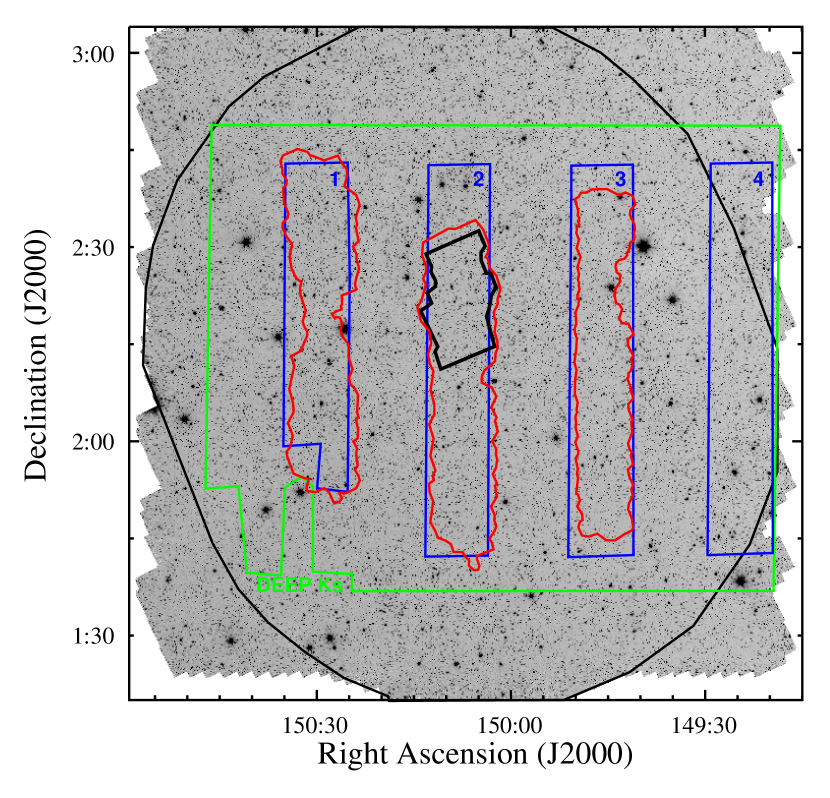
Figure 3: Layout of 3.6 $\mu$m survey coverage within the COSMOS field. A higher-resolution version is available in the published version of this article. The grayscale image is a shallow IRAC 3.6 $\mu$m mosaic built with exposures from all projects listed in Table 1 for illustration purposes. The linear stretch runs from $-0.05$ to 0.05 MJy sr^-1. The entire field was imaged by S-COSMOS. The large black ellipse indicates the approximate outer boundary of SPLASH-COSMOS. The green polygon encloses the UltraVISTA deep $K_{s}$ coverage. The four numbered blue polygons are the ultra-deep survey stripes. Red contours outline the regions with at least 25 hr of integration from SMUVS. Outside the red contours the depth of coverage smoothly declines to the $\sim 5$ hr SPLASH-COSMOS integration times. The black outline in the center of the field encloses the deep coverage from S-CANDELS, i.e., the area with at least 50 hr integration time.

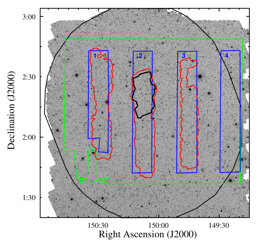
Figure 4: As Fig. 3, but showing the 4.5 $\mu$m survey coverage.

5 SMUVS Catalog Construction

5.1 Model PSF Generation

The SMUVS catalogs (Sec. 6) are based on point spread function (PSF)-fitting techniques implemented with StarFinder (Diolaiti et al. 2000), following analogous procedures to those used for SEDS (Ashby et al. 2013a). StarFinder uses scaled model PSFs to estimate source fluxes. For this reason, the first step in creating SMUVS catalogs is generating suitable model PSFs. Unlike S-CANDELS, which covered too small an area for reliable model PSFs to be constructed, each of the three SMUVS stripes included many stars suitable for PSF modeling. We chose to take advantage of SMUVS’ greater area coverage and generate new model PSFs to optimize our PSF-fitted photometry.

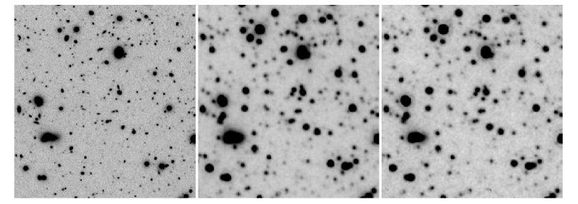
Figure 5: Three views of a small but typical SMUVS field to demonstrate the comparable sensitivities achieved by SMUVS and UltraVISTA. From left to right the panels show mosaics generated with the combined $HK_{s}$ images from UltraVISTA (Caputi et al. 2017), and at 3.6 and 4.5 $\mu$m for SMUVS. North is up and east is to the left. The field shown is approximately $100\times 120$ arcsec², and is located at 10:01:50, +2:00 in stripe 1.

The StarFinder algorithm for generating model PSFs can be distilled down to its essence in three parts. These are, first, identifying isolated, unsaturated field stars, second, generating cutout images centered on those stars and cleaning them of nearby contaminating sources, and third, scaling and median-stacking the cutout images. All cutouts were centered on the brightest PSF pixel. This procedure generated high-dynamic-range model PSFs with relatively high S/N ratios, that by construction reflect the spacecraft rotation angles at which the individual exposures were obtained. There is a limit to the fidelity of this procedure. Because the SMUVS AORs consisted of many small, deep maps (i.e., they did not individually cover the UltraVISTA stripes uniformly), the ensemble of rotation angles is a function of location within the stripes. Our technique, outlined below, generated ’stripe-average’ PSFs that do not fully reflect the small-scale variations. The limited visibility of the field, however – COSMOS is accessible to Spitzer only during windows $\sim$40 days long – means that the spacecraft can rotate only through a limited range of position angles, so our approach is a reasonable compromise between fidelity and convenience, as we show below.

We used only bright, unsaturated PSF stars observed with at least 25 hours total integration time to ensure their images reflected a representative distribution of position angles. In stripe 2, with its greater average integration time, we refined the model PSFs by iterating the StarFinder PSF stacking procedure on a version of the science mosaic from which contaminating field sources had been fitted and subtracted on a first pass, down to 5$\sigma$ significance. The procedure did not noticeably improve the PSFs for stripes 1 and 3 (it generated faint but broad artifacts in the extreme PSF wings), so in these fields the first-pass PSFs were adopted for the final catalogs.

All PSFs used here were post-processed to improve their suitability for photometry. Starfinder’s halo-smoothing feature was applied to suppress noise in the PSF outskirts. In addition, all PSF pixels farther than 64 pixels from the centroid were set to zero, and low-level artifacts remaining from the PSF construction process were eliminated by hand. These two steps prevented the iterative scaling-and-fitting procedure from introducing spurious features near the brighter sources. All PSFs images were subsequently normalized to unity total counts. As a sanity check they were then compared visually to the four-epoch PSF images generated by Caputi et al. (2017) and found to be broadly consistent, but with higher dynamic ranges. They were also larger, with 128-pixel diameters ($76\farcs 8$).

Ultimately we generated a total of six model PSF images, one for every combination of IRAC band and SMUVS stripe. The SMUVS PSFs are shown in Fig. 6. They have FWHMs of approximately 2″.

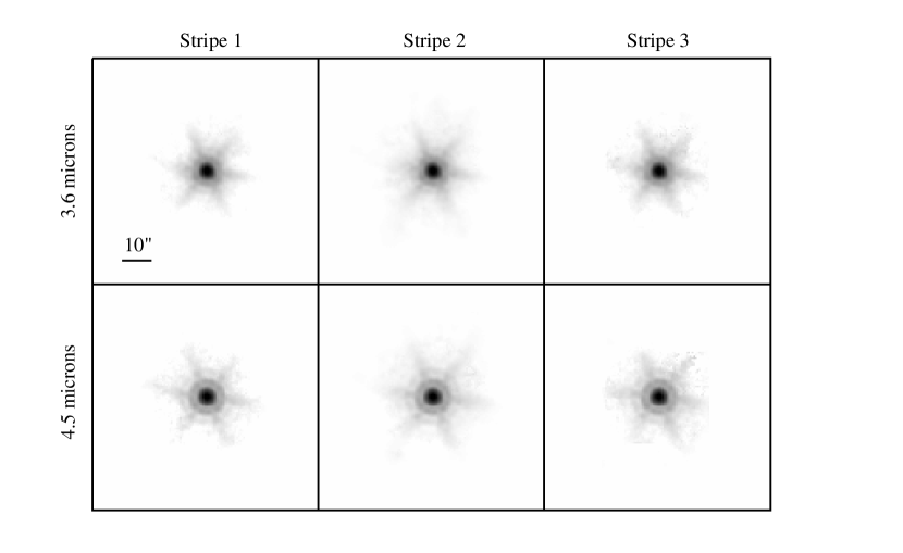
Figure 6: Montage of the PSFs derived from the full-mission SMUVS mosaics. These PSFs were used to construct the SMUVS catalogs. From left to right, PSFs are shown for UltraVISTA stripes 1 to 3. Each PSF image is 128 0$\farcs$6 pixels wide. The upper row shows the 3.6 $\mu$m PSFs derived by median-stacking of isolated unsaturated stars all of which were observed for at least 25 hr. The lower row shows their 4.5 $\mu$m equivalents. The inverse logarithmic stretch ranges from 0 to 0.03 in order to show faint structure such as the Airy rings; PSF peak values are roughly 0.06 for these normalized PSFs.

5.2 Source Extraction

To the greatest extent possible the SMUVS photometry was computed in the same way as was done earlier for SEDS and S-CANDELS, following the standard StarFinder procedure. In this scheme, the brightest source in the mosaic is identified and fitted with an appropriately scaled PSF to estimate its brightness. That source is then subtracted from the original image, and the process is repeated with the brightest source in the resulting residual image. By looping through this single-source fitting procedure until no significant detections remain in the residual, StarFinder generates a catalog of PSF-fitted estimated fluxes in brightness order. We ran iterated this process three times. On the first pass we set a 5$\sigma$ detection threshold. For the second and third passes StarFinder estimated the RMS from the source-subtracted mosaic, and could reach sources not detected in the original mosaic. We also set the detection threshold to 3$\sigma$ for the second and third passes to increase the sensitivity. Regions within $0.7\times$ the PSF FWHM were excluded from subsequent fits. Backgrounds were estimated locally for each source, within square regions $72\times$ the PSF FWHM on a side.

In all respects our StarFinder parameters were identical to those used for SEDS and S-CANDELS, with one exception. For those earlier efforts, regions nearer than $0.5\times$ the PSF FWHM of detected sources were excluded from fitting. Thus some sources in the SEDS and S-CANDELS catalogs may not, if heavily blended with a brighter companion, appear in the SMUVS catalogs, which are slightly more resistant to shredding of bright sources.

After the iterated fitting procedure was carried out on all three SMUVS stripes within the blue boundaries indicated in Figs. 3 and 4, aperture photometry was acquired at the positions of all StarFinder-detected sources. This was done by adding the scaled PSFs back into the residual images and photometering the resulting ’reconstituted’ sources within apertures of diameters 2$\farcs$4, 3$\farcs$6, 4$\farcs$8, 6$\farcs$0, 7$\farcs$2, and 12$\farcs$0. This technique permitted the photometry to be measured with less contamination from nearby sources and, because the nearby StarFinder-detected sources were by construction removed from the residual image used. The StarFinder PSFs were used to estimate and correct for flux falling outside the apertures.

The two resulting single-band IRAC catalogs for each stripe were then combined into a single two-band catalog using a position match with a 1″ search radius. The 1″ radius was selected because it is smaller than the FWHM of the IRAC PSF in either band, but larger than the 0$\farcs$7 exclusion radius around detected sources. After inspecting the catalogs, we chose to retain significant unmatched sources in order to improve the catalog completeness. Thus at faint levels, a significant fraction of the SMUVS detections are formally detected in only one IRAC band.

In summary, we have constructed one two-band position-matched catalog for each of the three SMUVS stripes. The catalogs are presented in Tables 2, 3, and 4. The catalogs contain a total of about 356,000 sources down to 4$\sigma$ limits of roughly 25.0 AB mag in both IRAC bands. The sensitivity limit accounts for both instrumental effects and the effects of source confusion.

5.3 The Impact of Source Confusion

Source confusion is significant at SMUVS depths. Indeed, it had a measurable (if marginal) impact even on the shallow counts in the SSDF (Ashby et al. 2013b). SMUVS is significantly deeper than SEDS (designed integration time of 12 hr, Ashby et al. 2013a; Fig. 2, bottom panel). We identified about 350,000 significant sources in the 0.66 deg² total SMUVS area, equivalent to roughly 10 beams per source, a level well above the 40 beams per source criterion for the onset of source confusion given in Rowan-Robinson (2001). Including fainter (less significant but nonetheless real) objects, of course, would raise the estimated source confusion accordingly. Accounting for source confusion was a primary motive behind our decision to use StarFinder in this work.

We used the COSMOS S-CANDELS observations to estimate the impacts of source confusion on SMUVS. The S-CANDELS survey provides a reliable means of dealing quantitatively with SMUVS source confusion for four reasons. First, S-CANDELS reaches fainter flux levels than SMUVS along the same general line of sight, and therefore accurately accounts for the behavior of real sources that SMUVS cannot detect reliably. Second, Spitzer’s short visibility windows for COSMOS mean that all IRAC observations of the field were taken at nearly identical spacecraft rotation angles, so the resulting PSFs are likewise nearly identical. Third, the SMUVS and S-CANDELS mosaics’ pixellation and tangent points were identical by construction. Thus the StarFinder source extraction simulations performed on the S-CANDELS mosaics by Ashby et al. (2015) are representative of the SMUVS source extractions at the same flux levels.

Source confusion dominates the photometric uncertainties for faint IRAC sources. Thus, the total uncertainties do not integrate down as the square root of the integration time as they would in the absence of confusion noise. As shown in Ashby et al. (2015), Fig. 15 and Table 3, the total uncertainty for COSMOS 3.6 $\mu$m sources photometered with StarFinder is 0.1 mag at 21.25 AB mag, but this only 0.02 mag greater (i.e., only roughly 20% more uncertain) than for sources that are brighter by a full magnitude or even more.

The tendency for confusion-dominated IRAC photometric uncertainties to grow slowly toward faint magnitudes has a somewhat non-intuitive consequence for source significance. For SMUVS in particular, a 25 mag (0.13 $\mu$Jy) source is a 4$\sigma$ detection. But a source half as bright (25.75 mag, 0.065 $\mu$Jy) is not a 2$\sigma$ detection – it is closer to 3$\sigma$. Users should bear this behavior in mind when using the SMUVS catalogs.

Table 2: Full-Depth Source Catalog for SMUVS Stripe 1

Object	RA,Dec	3.6 $\mu$m AB Magnitudes	3.6 $\mu$m Unc.	3.6 $\mu$m Coverage	3.6 $\mu$m Flag
	(J2000)	4.5 $\mu$m AB Magnitudes	4.5 $\mu$m Unc.	4.5 $\mu$m Coverage	4.5 $\mu$m Flag
SMUVS J100143.20+021729.0	150.43001,2.29139	9.64  9.60   9.52  9.48   9.45  9.44   9.44	0.03	748	1
		10.13 10.08  9.96  9.92   9.91  9.90   9.89	0.03	885	1
SMUVS J100210.51+015212.0	150.54377,1.87000	10.53 10.49 10.38 10.33 10.30 10.29 10.28	0.03	618	1
		11.05 11.00 10.89 10.85 10.83 10.82 10.81	0.03	622	1
SMUVS J100223.99+021604.6	150.59996,2.26795	10.54 10.51 10.40 10.36 10.35 10.34 10.33	0.03	201	1
		11.07 11.03 10.92 10.88 10.86 10.85 10.85	0.03	179	1
SMUVS J100157.37+020556.3	150.48904,2.09898	11.93 11.89 11.80 11.77 11.75 11.75 11.75	0.03	1362	0
		12.56 12.52 12.43 12.39 12.37 12.36 12.36	0.03	1420	0
SMUVS J100142.19+015320.0	150.42579,1.88888	12.40 12.36 12.29 12.25 12.23 12.23 12.23	0.03	884	0
		13.11 13.07 12.95 12.89 12.87 12.86 12.86	0.03	1054	0
SMUVS J100130.37+023616.1	150.37654,2.60446	12.41 12.37 12.29 12.26 12.24 12.24 12.24	0.03	522	0
		13.09 13.05 12.93 12.88 12.85 12.84 12.84	0.03	695	0
SMUVS J100152.83+021233.5	150.47012,2.20932	12.60 12.57 12.48 12.45 12.43 12.42 12.42	0.03	1571	0
		13.22 13.18 13.07 13.03 13.01 13.00 13.00	0.03	1590	0
SMUVS J100214.05+022416.0	150.55853,2.40444	12.64 12.61 12.54 12.50 12.49 12.48 12.48	0.03	402	0
		13.31 13.27 13.16 13.10 13.07 13.06 13.05	0.03	363	0
SMUVS J100125.93+020109.5	150.35805,2.01930	12.68 12.65 12.57 12.55 12.53 12.53 12.52	0.03	268	0
		13.44 13.39 13.27 13.20 13.17 13.16 13.15	0.03	301	0

Note. — The SMUVS catalog of IRAC-detected sources in Stripe 1. The sources are listed in magnitude order. This table is available in its entirety in a machine-readable form in the online journal. A portion is shown here for guidance regarding its form and content.

Table 3: Full-Depth Source Catalog for SMUVS Stripe 2

Object	RA,Dec	3.6 $\mu$m AB Magnitudes	3.6 $\mu$m Unc.	3.6 $\mu$m Coverage	3.6 $\mu$m Flag
	(J2000)	4.5 $\mu$m AB Magnitudes	4.5 $\mu$m Unc.	4.5 $\mu$m Coverage	4.5 $\mu$m Flag
SMUVS J100009.66+022349.0	150.04023,2.39693	11.11 11.08 11.02 10.98 10.97 10.97 10.97	0.03	1335	1
		11.71 11.66 11.55 11.52 11.51 11.50 11.49	0.03	496	1
SMUVS J100003.58+015044.9	150.01493,1.84579	11.60 11.56 11.49 11.46 11.44 11.43 11.42	0.03	436	1
		12.15 12.09 11.97 11.91 11.88 11.85 11.83	0.03	556	1
SMUVS J100057.12+023719.3	150.23798,2.62204	11.69 11.64 11.63 11.62 11.59 11.56 11.49	0.03	185	1
		11.52 11.47 11.36 11.31 11.29 11.28 11.27	0.03	58	1
SMUVS J100042.71+023941.6	150.17796,2.66155	11.88 11.83 11.72 11.70 11.69 11.67 11.62	0.03	375	1
		11.90 11.85 11.75 11.72 11.70 11.69 11.68	0.03	288	1
SMUVS J100028.36+023926.1	150.11818,2.65725	12.10 12.05 11.96 11.92 11.90 11.88 11.85	0.03	489	1
		12.25 12.20 12.14 12.11 12.10 12.09 12.08	0.03	274	1
SMUVS J100002.36+023259.5	150.00982,2.54987	12.65 12.62 12.55 12.53 12.52 12.51 12.52	0.03	36	1
		13.50 13.44 13.35 13.30 13.28 13.27 13.26	0.03	41	1
SMUVS J100032.55+020825.8	150.13564,2.14049	12.70 12.67 12.61 12.58 12.56 12.55 12.55	0.03	1535	1
		13.21 13.17 13.08 13.04 13.01 13.00 13.00	0.03	1345	1
SMUVS J100024.41+024422.6	150.10170,2.73961	12.92 12.87 12.79 12.74 12.71 12.69 12.67	0.03	292	1
		13.03 12.98 12.88 12.85 12.83 12.82 12.81	0.03	179	1
SMUVS J100057.88+023535.6	150.24118,2.59322	13.50 13.38 13.18 13.06 12.99 12.96 12.91	0.03	127	1
		13.07 13.03 12.94 12.89 12.86 12.84 12.83	0.03	32	1

Note. — The SMUVS catalog of IRAC-detected sources in Stripe 1. The sources are listed in magnitude order. This table is available in its entirety in a machine-readable form in the online journal. A portion is shown here for guidance regarding its form and content.

Table 4: Full-Depth Source Catalog for SMUVS Stripe 3

Object	RA,Dec	3.6 $\mu$m AB Magnitudes	3.6 $\mu$m Unc.	3.6 $\mu$m Coverage	3.6 $\mu$m Flag
	(J2000)	4.5 $\mu$m AB Magnitudes	4.5 $\mu$m Unc.	4.5 $\mu$m Coverage	4.5 $\mu$m Flag
SMUVS J095838.29+023010.2	149.65956,2.50284	8.86  8.82  8.76  8.72  8.71  8.70  8.69	0.03	539	1
		9.43  9.38  9.29  9.25  9.23   9.22  9.21	0.03	596	1
SMUVS J095858.28+022346.9	149.74282,2.39637	10.72 10.68 10.59 10.54 10.52 10.51 10.50	0.03	1179	1
		11.20 11.14 11.03 10.98 10.96 10.94 10.93	0.03	1041	1
SMUVS J095932.36+020032.7	149.88482,2.00909	11.08 11.05 10.96 10.92 10.91 10.90 10.89	0.03	256	1
		11.48 11.44 11.36 11.33 11.31 11.30 11.29	0.03	161	1
SMUVS J095852.55+023748.1	149.71896,2.63002	11.28 11.24 11.16 11.13 11.11 11.11 11.11	0.03	988	1
		11.82 11.77 11.68 11.64 11.61 11.60 11.60	0.03	956	1
SMUVS J095839.21+020905.6	149.66337,2.15154	12.60 12.56 12.50 12.47 12.45 12.45 12.44	0.03	411	0
		13.30 13.25 13.12 13.06 13.04 13.02 13.01	0.03	491	0
SMUVS J095833.72+014348.5	149.64051,1.73014	12.71 12.69 12.62 12.59 12.57 12.57 12.57	0.03	215	1
		13.53 13.48 13.34 13.28 13.25 13.24 13.23	0.03	213	1
SMUVS J095858.83+013746.1	149.74512,1.62947	12.89 12.86 12.79 12.76 12.74 12.74 12.74	0.03	184	1
		13.69 13.63 13.51 13.44 13.41 13.39 13.38	0.03	189	1
SMUVS J095920.69+022819.0	149.83621,2.47194	12.92 12.89 12.82 12.79 12.77 12.77 12.76	0.03	669	0
		13.64 13.59 13.47 13.41 13.38 13.37 13.35	0.03	475	0
SMUVS J095908.29+015732.6	149.78455,1.95906	12.94 12.91 12.84 12.81 12.79 12.79 12.79	0.03	1419	0
		14.78 14.58 14.32 14.13 13.97 13.90 13.82	0.03	860	0

Note. — The SMUVS catalog of IRAC-detected sources in Stripe 1. The sources are listed in magnitude order. This table is available in its entirety in a machine-readable form in the online journal. A portion is shown here for guidance regarding its form and content.

6 Catalog Format

Each SMUVS catalog follows an identical format. All IRAC sources detected with 4$\sigma$ significance in at least one IRAC band are included. The largest catalog section comes first, and lists all sources detected in both IRAC bands in brightness order. The entries for sources detected at 3.6 $\mu$m but not 4.5 $\mu$m, and also conversely, appear later. Invalid measurements are indicated with large negative numbers throughout.

The entry for each source includes its name and StarFinder-derived position. The positions given are those measured at 3.6 $\mu$m except for sources not detected in that band. For those sources the position measured at 4.5 $\mu$m is given instead.

Seven photometric measurements are given in each band for each detection. The first entry is always the PSF-fitted magnitude. The next six measurements are aperture magnitudes as described earlier. All photometry is stated in AB terms. The aperture photometry is corrected to total magnitudes following the same procedure used in Ashby et al. (2013a) in order to account for imperfect measurement of sky backgrounds in such a dense field. For SMUVS, the COSMOS-specific corrections were applied (Ashby et al. 2015, Fig. 15).

Uncertainty estimates are given for the 2$\farcs$4 diameter aperture photometry. These estimates are indicative of the uncertainties obtained for the PSF-fitted magnitudes as well, but should be regarded as underestimates for larger diameter apertures. Wider apertures suffer from two problems. First, the wider apertures can encompass extraneous features (e.g., faint undetected objects, artifacts, residuals from brighter nearby sources) that will reduce the precision of the photometry and bias it toward brighter magnitudes. Second, wider apertures necessarily have a higher contribution from shot noise.

The numbers of individual IRAC exposures taken at every source position, inferred from the coverage maps generated during mosaicking, are given in terms of 100 s exposures. The numbers given are measured at the cataloged positions of the sources. Because of artifact correction and cosmic ray rejection, these numbers can vary considerably even on arcsecond scales.

The data quality flags are described in Sec. 7.

7 Catalog Validation

The astrometric solution for IRAC is tied to the known positions of relatively bright point sources in the Two Micron All Sky Survey (2MASS; Skrutskie et al. 2006) Point Source Catalog. Recently, however, that astrometric solution was improved in two ways (Lowrance et al. 2016): first, by implementing a fifth-order polynomial to account for optical distortion; second, by accounting for the proper motions of bright 2MASS sources (which are significant for 22% of the 2MASS stars used in the pointing refinement) using the UCAC4 catalog (Zacharias et al. 2013). For SMUVS, the updated astrometric solution was used, so we verified the SMUVS astrometry against both 2MASS and SEDS – in other words, against the extremes of wide/shallow and deep/narrow coextensive observations in similar wavebands, and using IRAC astrometry measured with the earlier, third-order distortion correction. The positions of SMUVS sources are consistent with those from SEDS to within about 0$\farcs$12. Relative to 2MASS, the SMUVS source positions match to within about 0$\farcs$18 arcsec, consistent with what has been seen in earlier IRAC surveys.

Fig. 7 compares SMUVS photometry to that from SEDS, S-COSMOS, and Deshmukh et al. (2018). In all instances, the SMUVS photometry is consistent with previous measurements within the uncertainties, but the comparison reveals some systematic differences among the datasets, which are described here.

Comparison to Deshmukh et al. (2018): the SMUVS photometry is compared to that of Deshmukh et al. (2018) in all three UltraVISTA stripes and both IRAC bands in the top three rows of Fig. 7. Like SMUVS, Deshmukh et al. employ a PSF-fitting technique to photometer sources in the IRAC bands, but unlike SMUVS their photometry is measured at the positions of sources detected in a suite of very deep ground-based mosaics built by coadding exposures in the $J$ and $K_{s}$ bands. SMUVS sources were matched to those of Deshmukh et al. if their positions were coincident to within 0$\farcs$4. All SMUVS sources brighter than 25.5 mag at 3.6 and 4.5 $\mu$m, were considered. In addition, we required that the measured IRAC $[3.6]-[4.5]$ color in both catalogs had to agree to within 0.2 mag. This was done to help ensure that the photometry was compared for the same sources, which otherwise would have been problematic because the IRAC sources may resolve into multiple objects in the $HKs$-selected catalog.

For bright SMUVS sources (i.e., $[3.6]=[4.5]<16$ mag) the scatter in the comparison is very small in all three stripes and both bands, and appears dominated by systematic effects that are comparable to the roughly 3% uncertainty in the absolute calibration of the IRAC. This behavior is apparent in comparisons to SEDS and S-COSMOS as well. For sources fainter than 16 mag, considerably more scatter is apparent, but the mean deviations from zero difference (SMUVS-Deshmukh) tend to be comparable to the uncertainty in the absolute calibration error down to about 24 mag. For sources fainter than 24 mag, the difference between SMUVS and Deshmukh et al. is positive and larger than the systematic errors. We cannot definitively ascribe a cause to the discrepancy, but we speculate that it arises because the two catalogs are selected in different wavebands. Faint SMUVS sources may be systematically absent from Deshmukh et al. (which selects on $HK_{s}$), but may nonetheless satisfy our simple position and color-matching criteria, distorting the comparison in subtle ways.

Comparison to S-COSMOS: the SMUVS photometry is compared to that of S-COSMOS in rows 2-4 of Fig. 7, again for sources matched to within 0$\farcs$4. The comparison was done separately in the IRAC bands, down to the S-COSMOS detection limits of 1.0 and 1.7 $\mu$Jy in the 3.6 and 4.5 $\mu$m bands, respectively (23.9 and 23.3 AB mag). The comparison was based on S-COSMOS 1$\farcs$9 diameter aperture magnitudes, corrected to total magnitudes as specified in the S-COSMOS IRAC data delivery README file. Only S-COSMOS objects with data quality flags set to zero (i.e., good data) were used in the comparison.

The agreement between SMUVS and S-COSMOS for sources brighter than 23.5 mag is on average better than the 3% uncertainty in the absolute IRAC calibration. S-COSMOS sources fainter than 23.5 mag at 3.6 $\mu$m are systematically brighter on average in S-COSMOS than in SMUVS. This effect is not seen for the 4.5 $\mu$m S-COSMOS sources.

Comparison to SEDS: the SMUVS photometry is compared to that of SEDS in the bottom row of Fig. 7. For this comparison we used the 2$\farcs$4 diameter aperture magnitudes, corrected to total, from both SEDS and SMUVS. The agreement between SMUVS and SEDS is excellent at 3.6 $\mu$m. At 4.5 $\mu$m, an offset of about 0.06 mag is detected, in the sense that the SMUVS photometry is on average systematically 0.06 mag fainter for sources fainter than about 18 mag. The origin of this systematic offset is not understood.

The bottom row of Fig. 7 compares SMUVS sources in a single 0.5 mag bin fainter than our nominal 4$\sigma$ cutoff at 25 mag. Such sources appear on average to be brighter by about 0.2 mag in SEDS than in SMUVS, with a comparable uncertainty. The reason for the difference is not entirely clear, because at this magnitude confusion noise dominates the uncertainties in both catalogs. We speculate that it may result from the slightly different selection function used for SMUVS. Whereas the SMUVS catalogs include single-band $4\sigma$ detections but discard faint off-band detections, the SEDS catalogs include (somewhat less significant) detections in both bands. This could lead to a situation where sources in the shallower SEDS mosaics tend to be boosted by noise fluctuations slightly more often than for SMUVS, resulting in the red average color seen in the faintest bins of the bottom row Fig. 7.

Figure 7: Comparisons of SMUVS photometry to previously published results. All points indicate means of magnitude differences for position-matched sources, measured in bins 0.5 mag wide. The error bars are $1\sigma$. Top three rows: SMUVS photometry for stripes 1, 2, and 3 separately compared to that from UltraVISTA using $HK_{s}$ priors, from Deshmukh et al. (2018). Vertical dashed lines indicate the UltraVISTA 80% completeness limit. Next three rows: SMUVS photometry compared to coextensive S-COSMOS 1$\farcs$9 diameter aperture photometry (Sanders et al.  2007) down to the S-COSMOS detection thresholds, indicated by the vertical dashed lines. Bottom row: SMUVS compared to SEDS (Ashby et al. 2013a). The comparison to S-COSMOS was based on SMUVS 2$\farcs$4 diameter aperture photometry, and the comparison to SEDS was based on SMUVS and SEDS bias-corrected PSF-fitted magnitudes.

The colors of IRAC sources as measured by SMUVS are also consistent with what has been seen in other surveys. In Fig. 8 we plot the [3.6]$-$[4.5] color of all SMUVS sources detected in both IRAC bands and having 3.6 $\mu$m magnitudes between 22 and 25.5 AB mag. The behavior of these color distributions is essentially identical to what has been seen before by, e.g., S-CANDELS (Ashby et al. 2015), in particular it produces both the bimodal color distribution typically seen for relatively bright sources and the trend toward a redder, single-mode distribution at fainter fluxes.

Figure 8: The IRAC color distributions of sources detected in both warm IRAC bands by SMUVS.

The 14th and last columns of the three SMUVS catalogs contain data quality flags for the 3.6 and 4.5 $\mu$m photometry, respectively. A flag of zero indicates no known issues with the photometry. Photometry for some sources was potentially corrupted by the large halos around bright stars, which may have compromised the ability of StarFinder to reliably estimate the local backgrounds. Sources potentially affected by background contamination have been assigned a data quality flag of 1. All cataloged sources having only single-band detections are also flagged. A flag of 2 indicates a bright ($>23.0$ mag) single-band detection. Given the well-documented color distribution of IRAC-detected sources, which is reproduced by SMUVS (Fig. 8), it is implausible that such bright sources (if real) would be absent in the off-band. Instead, as we have verified by inspection, such detections are artifacts of the shredding of extended sources. A flag of 3 indicates a different single-band detection, i.e., a faint ($<23.0$ mag) one. Unlike the bright single-band detections, faint sources can be real, and arise when red or blue IRAC colors push the off-band flux below the SMUVS detection threshold. It is apparent by inspection, many such single-band detections are indeed apparent in the off-band, but at such low signal-to-noise ratios that they are not formally detected by StarFinder.

7.1 Limitations of the SMUVS Catalogs

The SMUVS catalog is not optimal for extended sources. Such objects are likely to be ’shredded’ into multiple objects by the iterated PSF-fitting procedure. Users should be cautious about SMUVS photometry of bright, extended sources. As noted above, shredded sources can appear in the SMUVS catalogs as single-band detections, because extended sources are unlikely to be modeled by StarFinder with spatially registered point sources in both bands. We have flagged high-SNR but unmatched sources in the catalog so indicate that they likely arise from shredded objects. Other unmatched sources are undoubtedly real, as corroborated by how closely the SMUVS source counts follow the deeper completeness-corrected counts from S-CANDELS (Fig. 9), down to 25 AB mag; these objects are ’lost’ from the off-band because of their colors. Users of the SMUVS catalogs are cautioned to make use of the data quality flags and to take the proximity of bright sources into account when interpreting the photometry.

Sources fainter than about 23 AB mag will not be impacted by shredding, but brighter sources could be if they are extended. An attempt has been made to correct the SMUVS photometry in a statistical sense for modestly extended sources, following Ashby et al. (2013a), but this approach will be inadequate for sources that are broader than 1–2$\times$ the IRAC FWHM. Users can examine the curve of growth through the SMUVS apertures as a means of verifying the photometry for individual sources. Well-characterized sources will have aperture magnitudes that agree with each other, and with the PSF-fitted photometry.

The SMUVS catalog is not the best source of photometry for especially bright sources even if they are pointlike. To most efficiently photometer the faint, distant galaxies that are the primary objectives for SMUVS, it was necessary to adopt a length scale on which to model the variations seen the backgrounds of the SMUVS mosaics. The length scale chosen – 72$\times$ the FWHM of the PSFs used for photometry – was a compromise between the competing needs to accurately fit both bright stars’ outskirts and background variations. As a result, the magnitudes for Milky Way stars brighter than $\sim$13 AB mag are systematically underestimated to varying degrees.

The SMUVS counts are shown in Fig. 9 and Table 5. They appear broadly consistent with number counts based on UltraVISTA $HK_{s}$ priors (Deshmukh et al. (2017) down to $\sim$24.5 mag, at which point incompleteness begins to have an impact. At bright magnitudes the SMUVS counts closely follow the Milky Way star counts model derived from DIRBE observations toward COSMOS (Arendt et al. 1998), except for very bright sources which are impacted by small number statistics. The dashed lines shown in Fig. 9 are not fits to the counts. At fainter magnitudes the counts closely follow the so-called ’default’ model from Helgason et al. (2012). The SMUVS counts follow a linear trend all the way from the ’knee’ of the counts at 20 AB mag to faint count levels, where they depart from the ’default’ model at roughly [3.6]=25 and [4.5]=24.5 AB mag. We infer that the SMUVS counts begin to suffer from significant incompleteness at about these levels. By comparison, the not-completeness-corrected counts shown for COSMOS in Figs. 17c and 18c of Ashby et al. (2015) depart from this trend at brighter magnitudes. It therefore appears that the SMUVS catalogs are complete to significantly fainter levels than the earlier catalogs built for the COSMOS field.

Finally, users can refer to the IRAC color distributions in Fig. 8 as indicators of valid photometry. Most (not all) sources with valid photometry will have IRAC colors in the range $-0.5<[3.6]-[4.5]<0.5$. If a cataloged SMUVS object has an IRAC color with an absolute value greater than unity, the underlying IRAC photometry should be treated with caution.

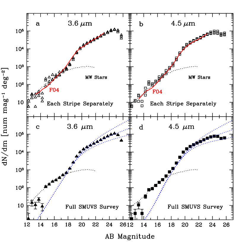
Figure 9: Differential source counts in the COSMOS field measured in both warm IRAC bands by SMUVS. Open symbols show the counts for individual stripes, while solid symbols indicate the counts summed over all three SMUVS stripes. Error bars represent only the Poisson statistics arising from the numbers of galaxies in each magnitude bin. The red lines in panels (a) and (b) indicate the incompleteness-corrected counts measured in the EGS by Fazio et al. (2004b). The dotted lines indicate estimated counts arising from Milky Way stars in COSMOS specifically, based on the DIRBE Faint Source Model at 3.5 and 4.9 $\mu$m (Arendt et al. 1998; Wainscoat et al. 1992; Cohen 1993, 1994, 1995). The blue dotted lines in the lower panels indicate the Helgason et al. (2012) model counts for those bands. In both cases the IRAC counts closely follow the middle trend until rather faint magnitudes even in the absence of completeness corrections, which have not been applied.

Table 5: Deep Source Counts in the IRAC Bands

Mag	3.6 $\mu$m		4.5 $\mu$m
(AB)	Counts	Unc	Counts	Unc
13.25	1.032	0.188	1.032	0.188
13.75	1.333	0.129	0.555	0.383
14.25	0.953	0.209	1.509	0.104
14.75	2.053	0.055	1.887	0.067
15.25	2.188	0.047	1.944	0.062
15.75	2.340	0.039	2.123	0.051
16.25	2.421	0.036	2.299	0.041
16.75	2.553	0.031	2.450	0.035
17.25	2.704	0.026	2.657	0.027
17.75	2.831	0.022	2.887	0.021
18.25	3.073	0.017	3.079	0.017
18.75	3.413	0.011	3.382	0.012
19.25	3.749	0.008	3.705	0.008
19.75	3.989	0.006	3.994	0.006
20.25	4.157	0.005	4.179	0.005
20.75	4.272	0.004	4.309	0.004
21.25	4.372	0.004	4.410	0.004
21.75	4.471	0.003	4.504	0.003
22.25	4.573	0.003	4.589	0.003
22.75	4.676	0.003	4.689	0.003
23.25	4.784	0.002	4.776	0.002
23.75	4.881	0.002	4.851	0.002
24.25	4.982	0.002	4.892	0.002
24.75	5.038	0.002	4.877	0.002
25.25	4.959	0.002	4.760	0.002
25.75	4.647	0.003	4.793	0.002

Note. — Differential number counts in the COSMOS field as measured in the three SMUVS stripes in both operable IRAC bands, expressed in terms of log$(N)$ mag^-1 deg^-2. Uncertainties are 1$\sigma$ estimates based solely on the number of sources in each bin, and do not reflect calibration errors, systematic effects or incompleteness corrections, which were not applied.

References

- Arendt et al. (1998) Arendt, R G., et al. 1998, ApJ, 508, 74
- Ashby et al. (2009) Ashby, M. L. N., Stern, D., Brodwin, M., et al. 2009, ApJ, 701, 428
- Ashby et al. (2013) Ashby, M. L. N., Willner, S. P., Fazio, G. G., et al. 2013a, ApJ, 769, 80
- Ashby et al. (2013) Ashby, M. L. N., Stanford, S. A., Brodwin, M., et al. 2013b, ApJS, 209, 22
- Ashby et al. (2015) Ashby, M. L. N., Willner, S. P., Fazio, G. G., et al. 2015, ApJS, 218, 33
- Barmby et al. (2008) Barmby, P., Huang, J.-S., Ashby, M. L. N., et al. 2008, ApJS, 177, 431-445
- Bell & de Jong (2001) Bell, E. F., & de Jong, R. S. 2001, ApJ, 550, 212
- Caputi et al. (2011) Caputi, K. I., Cirasuolo, M., Dunlop, J. S., et al. 2011, MNRAS, 413, 162
- Caputi (2013) Caputi, K. I. 2013, ApJ, 768, 103
- Caputi (2014) Caputi, K. I. 2014, International Journal of Modern Physics D, 23, 1430015
- Caputi et al. (2014) Caputi, K. I., Michałowski, M. J., Krips, M., et al. 2014, ApJ, 788, 126
- Caputi et al. (2015) Caputi, K. I., Ilbert, O., Laigle, C., et al. 2015, ApJ, 810, 73
- Caputi et al. (2017) Caputi, K. I., Deshmukh, S., Ashby, M. L. N., et al. 2017, ApJ, 849, 45
- Cohen et al. (1993) Cohen, M., et al. 1993, AJ, 105, 1860
- Cohen et al. (1994) Cohen, M., et al. 1994, AJ, 107, 582
- Cohen et al. (1995) Cohen, M., et al. 1995, ApJ, 444, 874
- Dalton et al. (2006) Dalton, G. B., Caldwell, M., Ward, A. K., et al. 2006, Proc. SPIE, 6269, 62690X
- Damen et al. (2011) Damen, M., Labbé, I., van Dokkum, P. G., et al. 2011, ApJ, 727, 1
- Dekel et al. (2009) Dekel, A., Birnboim, Y., Engel, G., et al. 2009, Nature, 457, 451
- Deshmukh et al. (2017) Deshmukh, S., Caputi, K. I., Ashby, M. L. N., et al. 2017, arXiv:1712.03905
- Diolaiti et al. (2000) Diolaiti, E., et al. 2000, Proc. SPIE, 4007, 879
- Emerson & Sutherland (2010) Emerson, J. P., & Sutherland, W. J. 2010, Proc. SPIE, 7733, 773306
- Fang et al. (2004) Fang, F., Shupe, D. L., Wilson, G., et al. 2004, ApJS, 154, 35
- Fazio et al. (2004a) Fazio, G. G., Hora, J. L., Allen, L. E., et al. 2004, ApJS, 154, 10
- Fazio et al. (2004b) Fazio, G. G., Ashby, M. L. N., Barmby, P., et al. 2004, ApJS, 154, 39
- Helgason et al. (2012) Helgason, K., Ricotti, M., & Kashlinsky, A. 2012, ApJ, 752, 113
- Hopkins et al. (2006) Hopkins, P. F., Hernquist, L., Cox, T. J., Robertson, B., & Springel, V. 2006, ApJS, 163, 50
- Ilbert et al. (2010) Ilbert, O., Salvato, M., Le Floc’h, E., et al. 2010, ApJ, 709, 644
- Ilbert et al. (2013) Ilbert, O., McCracken, H. J., Le Fèvre, O., et al. 2013, A&A, 556, A55
- Krick et al. (2009) Krick, J. E., Surace, J. A., Thompson, D., et al. 2009, ApJS, 185, 85
- Koekemoer et al. (2007) Koekemoer, A. M., Aussel, H., Calzetti, D., et al. 2007, ApJS, 172, 196
- Labbé et al. (2013) Labbé, I., Oesch, P. A., Bouwens, R. J., et al. 2013, ApJ, 777, L19
- Lacy et al. (2004) Lacy, M., Storrie-Lombardi, L. J., Sajina, A., et al. 2004, ApJS, 154, 166
- Laigle et al. (2016) Laigle, C., McCracken, H. J., Ilbert, O., et al. 2016, ApJS, 224, 24
- Lin et al. (2012) Lin, L., Dickinson, M., Jian, H.-Y., et al. 2012, ApJ, 756, 71
- Lonsdale et al. (2003) Lonsdale, C. J., Smith, H. E., Rowan-Robinson, M., et al. 2003, PASP, 115, 897
- Lonsdale et al. (2004) Lonsdale, C., Polletta, M. d. C., Surace, J., et al. 2004, ApJS, 154, 54
- Lowrance et al. (2016) Lowrance, P. J., Carey, S. J., Surace, J. A., et al. 2016, Proc. SPIE, 9904, 99045Z
- Malhotra et al. (2005) Malhotra, S., Rhoads, J. E., Pirzkal, N., et al. 2005, ApJ, 626, 666
- Mauduit et al. (2012) Mauduit, J.-C., Lacy, M., Farrah, D., et al. 2012, PASP, 124, 714
- McCracken et al. (2012) McCracken, H. J., Milvang-Jensen, B., Dunlop, J., et al. 2012, A&A, 544, A156
- Milvang-Jensen et al. (2013) Milvang-Jensen, B., Freudling, W., Zabl, J., et al. 2013, A&A, 560, A94
- Muzzin et al. (2013) Muzzin, A., Marchesini, D., Stefanon, M., et al. 2013, ApJ, 777, 18
- Papovich et al. (2016) Papovich, C., Shipley, H. V., Mehrtens, N., et al. 2016, ApJS, 224, 28
- Rix et al. (2004) Rix, H.-W., Barden, M., Beckwith, S. V. W., et al. 2004, ApJS, 152, 163
- Rowan-Robinson (2001) Rowan-Robinson, M. 2001, ApJ, 549, 745.
- Sánchez et al. (2017) Sánchez, P., Lira, P., Cartier, R., et al. 2017, arXiv:1710.01306
- Sanders et al. (2007) Sanders, D. B., Salvato, M., Aussel, H., et al. 2007, ApJS, 172, 86
- Schuster et al. (2006) Schuster, M. T., Marengo, M., & Patten, B. M. 2006, Proc. SPIE, 6270, 65
- Scoville et al. (2007) Scoville, N., Aussel, H., Brusa, M., et al. 2007, ApJS, 172, 1
- Shapley et al. (2006) Shapley, A. E., Steidel, C. C., Pettini, M., Adelberger, K. L., & Erb, D. K. 2006, ApJ, 651, 688
- Skrutskie et al. (2006) Skrutskie, M. F., Cutri, R. M., Stiening, R., et al. 2006, AJ, 131, 1163
- Somerville et al. (2008) Somerville, R. S., Hopkins, P. F., Cox, T. J., Robertson, B. E., & Hernquist, L. 2008, MNRAS, 391, 481
- Stefanon et al. (2015) Stefanon, M., Marchesini, D., Muzzin, A., et al. 2015, ApJ, 803, 11
- Steinhardt et al. (2014) Steinhardt, C. L., Speagle, J. S., Capak, P., et al. 2014, ApJ, 791, L25
- Stern et al. (2005) Stern, D., Eisenhardt, P., Gorjian, V., et al. 2005, ApJ, 631, 163
- Timlin et al. (2016) Timlin, J. D., Ross, N. P., Richards, G. T., et al. 2016, ApJS, 225, 1
- Wainscoat et al. (1992) Wainscoat, R., et al. 1992, ApJS, 88, 529
- Werner etal. (2004) Werner, M. W., Roellig, T. L., Low, F. J., et al. 2004, ApJS, 154, 1
- Zacharias et al. (2013) Zacharias, N., Finch, C. T., Girard, T. M., et al. 2013, AJ, 145, 44