Towards General Distributed Resource Selection

Abstract

The advantages of distributing workloads and utilizing multiple distributed resources are now well established. The type and degree of heterogeneity of distributed resources is increasing, and thus determining how to distribute the workloads becomes increasingly difficult, in particular with respect to the selection of suitable resources. We formulate and investigate the resource selection problem in a way that it is agnostic of specific task and resource properties, and which is generalizable to range of metrics. Specifically, we developed a model to describe the requirements of tasks and to estimate the cost of running that task on an arbitrary resource using baseline measurements from a reference machine. We integrated our cost model with the Condor matchmaking algorithm to enable resource selection. Experimental validation of our model shows that it provides execution time estimates with 157–171% error on XSEDE resources and 18–31% on OSG resources. We use the task execution cost model to select resources for a bag-of-tasks of up to 1024 GROMACS MD simulations across the target resources. Experiments show that using the model’s estimates reduces the workload’s time-to-completion up to $\sim$85% when compared to the random distribution of workload across the same resources.

I Introduction

The Worldwide Large Hadron Collider Grid (WLCG) was created to support multiple experiments at LHC that collect and distribute hundreds of petabytes of data worldwide to hundreds of computer centers. The WLCG has become one of the prototypical example of utilizing distributed and heterogeneous resources for scientific computing. There are many other large scale experimental and observation facilities—SKA, LSST, DUNE to name just a few—that also require multiple heterogeneous resources, although the number and type of resources varies.

The workloads from these experiments are often expressed as a collection of tasks. Historically, these experiments have placed tasks on different resources using implicit assumptions about resources and task properties. The types of tasks and distributed resources that need to be federated is changing; however, existing customized algorithms and approaches are not easily generalizable, nor extensible.

The availability of multiple distributed resources, often with diverse capabilities, offers the opportunity to improve resource utilization and increase the concurrency of workload execution. The benefits of distributing the execution of a workload across several types of resources has been investigated [1, 2], however, a consequence of the increase in the number and types of distributed resources is the resource selection problem. This problem can be formulated as: “The selection of a subset of resources to execute a workload among those available to a user”. Resource selection is composed of two questions: one question is of resource viability, which asks “Which resources can be used to execute the given workload?”; the other is of execution affinity, which asks “Which available resources should be used in the execution of the workload?”.

The resource viability problem has been addressed by [3], which provided a general method that uses the requirements of tasks and capabilities of a resource to determine whether a resource can successfully execute the task. The execution affinity problem has been investigated using application benchmarks comprised of a pre-defined suite of applications to provide an understanding on how resources perform [4]. However, further work is required to standardize the process by which performance data is measured, analyzed, reported and interpreted [4]. Workload scheduling algorithms [5, 6] either implicitly need to solve the execution affinity problem, or require it to be solved. These algorithms need knowledge of the cost of executing each task on each viable resource. Approaches to estimate task execution costs either require information on the task’s code structure and hardware architecture, or historical data on the cost of running each task on the possible target resources.

Several studies compare different types of applications and resources, and how different applications can exploit different types of resources [7, 8, 9]. However, there are no general models for the resource selection problem, or published results benchmarking them compared to a random selection of resources. Thus, not surprisingly, there do not exist quantitative estimates of improvements arising from resource selection as a function of scale (number of tasks and resources), or the degree of heterogeneity. Last but not least, resource selection methods have been tightly integrated with specific software tools, making comparisons across resource selection algorithms intractable.

Against this backdrop and its increasing importance, we investigate the generalized distributed resource selection problem. We focus on a class of problems that have not historically utilized distributed resources: A large fraction of the approximately half a million single core jobs submitted to XSEDE are MD simulations using community codes such as GROMACS, AMBER and CHARMM. These simulations are typically bound to a specific resource at the time of job submission. Assuming resources are fungible, the suitable selection of resources raises the theoretical possibility of reducing the time-to-completion of the tasks and improving the overall throughput of the collective set of XSEDE resources. This requires selecting resources that allow to take advantage of lower queue waiting times while not incurring into a higher execution waiting time, or vice versa. Both scenarios reiterate the importance of resource selection for the collective utilization of distributed computing resources.

In this paper, we formulate and investigate the resource selection problem that is agnostic of specific task and resource properties, and which is generalizable to a range of metrics (such as monetary cost, execution time etc.). Specifically, we propose a task execution cost model which can predict the cost of executing a task on a resource. We incorporate this model into the Condor matchmaking process to distribute workloads across resources. Using our model, we use historical information of the execution times of a singly-threaded GROMACS MD simulation running on a baseline cluster (Amarel) to predict the execution times of the same simulation on the different resources: XSEDE (Bridges, Comet, SuperMIC) and the XSEDE OSG virtual organization (or OSG in short). Our experiments show that our model provides execution time estimates with 157–171% error on XSEDE resources and 18–31% on OSG when we do not consider any information about the instruction-level parallelism the simulation exploits during execution. We use the task execution cost model to select resources for a bag-of-tasks of up to 1024 GROMACS MD simulations across the target resources. Experiments show that using the model’s estimates reduces the workload’s time-to-completion up to $\sim$85% when compared to the random distribution of workload across the same resources.

II Related Work

The resource selection problem has been actively studied by the HTC community. Due to the heterogeneity and transience of the resources composing an HTC DCR, the processed of resource selection used by the HTC community primarily focuses on: (i) standardizing how jobs and resources are described [10, 11, 12, 13, 14]; (ii) providing ways to discover the resources available in a HTC DCR [15, 16]; and (iii) providing a general method, known as matchmaking, to match jobs with resources that satisfy their requirements [17]. Often, the process of matchmaking is carried out by resource brokers [18, 19, 20, 21].

Application benchmarking is most often related to the problem of estimating the performance of an application workload on a given resource of group of resources. Application benchmarks provide insights into how a specific resource performs when executing a predefined application workload. The use of application benchmarks [19, 22] to express the requirements of a workload has been shown to improve the performance of the matchmaking process. However, given the state-of-the-art, much effort is still required to standardize how to measure, analyze and report benchmark results [4]. Without such a standardization, comparison and interpretation of benchmarks across multiple resources remains difficult.

Work has been done on providing bounds or estimates on the worst-case execution times of an application workload on a given resource [23, 24, 25]. Given a workload with a set of tasks, deterministic methods for timing analysis analytically derive an upper bound on the execution time of each task, based on hardware specifications and tasks’ code structure [23]. Probabilistic timing analysis use both static and measurement-based methods, executing workload’s tasks on the hardware of a resource with a predefined set of inputs to estimate the worst-case execution time of the task.

Deterministic and probabilistic timing analyses suffer from limitations related to the amount and accuracy of the information they require, or to the strength of their assumptions. Deterministic methods require detailed knowledge of the resource’s hardware and of the task’s code structure; probabilistic analyses using static methods assume information on the task’s code structure [23]; and probabilistic analyses using measurement-based methods do not assume any information on software internals, but place strong assumptions on the hardware and on how observations are taken [24, 26]. Collecting the required information or matching the assumptions made by these methods is challenging if not infeasible when considering selections over multiple production-grade resources.

There have also been efforts to predict task execution time on a resource using least-squares [27], k-Nearest Neighbors [28], iverson1996runneural networks [29] maximum likelihood estimation and random forests [30]. These methods require historical information of similar runs to generate predictions, and are considered a convenient way to estimate the cost of executing a task on a resource. However, there is limited availability of extensive and consistent collections of historical data about the execution costs of workloads running on production-grade resources. This reduces the usefulness of these methods for real-life use-cases, especially when considering resource selection among multiple resources.

III Resource Selection

We address the resource selection problem by devising a model to predict the cost of executing a given task on a given resource. We use this prediction, alongside other type of information when available, to choose resources that are more likely to optimize a given metric. In this way, we frame the resource selection problem as follows: Given a set of tasks, a set of resources, and a metric of performance, the resource selection problem consists in selecting the resources that optimize the given metric when executing the given tasks.

The predictions of our model use baseline measurements on a single reference resource and require no information about the structure of the code executed on that resource. We execute each task of a workload application on a resource, collecting data about its performance. On the base of these data, we analytically predict the cost of executing those tasks on an arbitrary resource. In this way, we avoid to execute and measure the performance of the same set of tasks on multiple resources.

We predict the cost of executing a task on a resource without using information about the structure of the task’s code and without detailed information about the resource’s hardware architecture. In this way, we trade off between simplifying the process of collecting the data required to predict the cost of execution and the accuracy of that prediction. Lack of accuracy is acceptable as far as the model’s predictions support effective resource selection for the distributed execution of a given workload over a given set of resources.

III-A Cost Model of Task Execution

The key idea of our cost model of task execution is to explicitly define the functionalities which a task uses during its execution. We define a consumable to be the entity that represents a functionality from a resource which a task uses during its execution. We show that we can calculate the cost of executing a task on a resource based on the consumables the task uses to run to completion, and on the cost of using each consumable on a resource.

We formally define task, workload, and resource in terms of consumables, and provide a model to estimate the cost of executing a task. Cost evaluation can be based on multiple units of measurements such as quantity of allocation, currency, or energy. To simplify the construction of our model, we assume: (1) tasks use required consumables independent from the resource that offer them; and (2) the cost of using any consumable offered by a resource is fixed. Here the terms we define from first principles:

Consumable:

An entity representing a unit of work. A consumable has two properties: (1) type, which determines the kind of work the entity can perform; and (2) form, which specifies the conditions that must be satisfied for the consumable to be used to perform work.

Requirement:

Amount of a consumable, where the amount is assumed to be fixed.

Instruction:

Set of tuples, each specifying a certain requirement.

Task:

Sequence of instructions, executed in the order specified by the sequence.

Workload:

Set of tasks, where all tasks can run concurrently.

Capability:

Rate at which a consumable is offered, assumed to be fixed.

Resource:

Set of tuples, each specifying a certain capability.

Formally, a consumable $c$ is a set $\{type,form\}$, where $type$ is a single value while $form$ is a set of pairs. For any pair in $form$, the first element is an attribute $attr$ that uniquely identifies the pair in $form$; the second element of the pair is a condition $cond$, expressed as a set of values, that specifies how $c$ can be used. A requirement $req$ is a tuple $(c,amt)$ where $c$ is a consumable and $amt>0$ is fixed amount of that consumable. An instruction $ins$ is a set $\{req_{1},\ldots,req_{n}\}$, where each requirement $req_{n}$ specifies the amount of a consumable required by $ins$. A task $task$ is a sequence of instructions $[ins_{1},\ldots,ins_{n}]$, where $|ins_{i}|$ is the number of requirements of each instruction $ins_{i}$.

Let $C$ be the set of $m$ distinct consumables, where each consumable is specified by a requirement of an instruction in $task$. For each $c\in C$, we calculate the total amount $amt_{c}$ of consumable $c$ required by the instructions in $task$ by taking the sum of the amounts specified by any requirement of any instruction that also specifies $c$ as its consumable. We express $amt_{c}$ as:

$$amt_{c}=\sum_{i=1}^{n}\sum_{j=1}^{|ins_{i}|}ins_{i}.ireq_{j}.amt\cdot\mathbbm{1}_{\{\begin{subarray}{c}ins_{i}.ireq_{j}.c=c\end{subarray}\}},$$ (1)

where $\mathbbm{1}$ is the indicator function, which equals 1 if the consumable specified by the $j$-th requirement of the $i$-th instruction of $task$ is $c$, and 0 otherwise. We call Eq. 1 the aggregation procedure.

We can now define task $task$ also as a set $\{req_{1},\ldots,req_{n}\}$, where each requirement $req_{n}$ specifies the total amount of consumable $c\in C$ required by the instructions of $task$. It is important to note that the aggregation procedure discards information on the order (and concurrency) with which the task’s instructions can use consumables, but provides a simple representation of a task’s requirements. We define a workload $WL$ as a set of tasks $\{task_{1},\ldots,task_{n}\}$.

We define a capability $cap$ as a set $\{c,rate\}$, where $c$ is a consumable and $rate>0$ is fixed. $rate$ represents the number of consumables offered per unit of cost (e.g., in terms of time, money, or energy). In this way we establish a relationship between the use of a consumable and the cost of using a consumable. We define a resource $res$ as a set $\{cap_{1},\ldots,cap_{n}\}$, where each capability $cap_{n}$ offers the use of a unique consumable at a fixed rate.

Assuming that a given task can run on a given resource, we define the cost $K$ of running a task on a resource as the total cost required to sequentially consume the amounts of consumables specified by the task requirements, at the rate offered by the corresponding resource capabilities. The cost of running the task on a resource is expressed sequentially because our model does not consider the order (or concurrency) with which tasks can use consumables, nor our model takes into account the order in which the resource offers consumables.

Formally, let there be a task $task=(req_{1},\ldots,req_{n})$ and resource $res=(cap_{1},\ldots,cap_{n})$. Then, $K$ is defined as:

$$K=\sum_{i=1}^{m}\sum_{j=1}^{n}\frac{req_{i}.amt}{cap_{j}.rate}\mathbbm{1}_{\{\begin{subarray}{c}req_{i}.c=cap_{j}.c\end{subarray}\}}$$ (2)

III-B Resource Selection Process

We decompose the problem of resource selection in two subproblems: (1) selecting viable resources to execute a given workload; and (2) selecting a subset of these resources that can execute the given workload, optimizing a given metric of performance. We first adapt the Condor matchmaking algorithm to operate in terms of consumables; we call the resulting algorithm the ‘adapted matchmaking algorithm’ (AMA). We then show that it is possible, but not necessary, for the AMA to select resources based on requirements and capabilities.

III-B1 Resource Viability

To adapt the Condor matchmaking algorithm to operate in terms of consumables, we define the algorithms $SATISFY\_REQ$ and $SATISFY\_TASK$ to determine whether a resource can execute a task. $SATISFY\_REQ$ (Alg. 1) takes as input a requirement and capability and determines whether the consumable specified by the capability can be used to satisfy the requirement. $SATISFY\_REQ$ checks whether: (1) the types of consumables of the requirement and capability are the same; (2) for every form attribute in the requirement there is a corresponding form attribute in the capability; and (3) for each form attribute that is in both the requirement and the capability there is a form condition in the capability that is also a form condition in the requirement. Note that the comparison operator used to decide whether two values are equal depends on the data type of the values (e.g., integer, float, string), as discussed in several specifications [10, 11].

Algorithm 1 Check if capability (cap) consumable can be used to satisfy requirement (req)

1:req; cap

2:True or False

3:procedure satisfy_req(req, cap)

4:     if req.c.type != cap.c.type then

5:         return False      

6:     for all (attr, cond) in req.c.form do

7:         if attr not in cap.c.form then

8:              return False          

9:         if cap.c.form.cond $\cap$ cond $\emptyset$ then

10:              return False               

11:     return True

$SATISFY\_TASK$ (Alg. 2) takes as input a task and resource and checks whether for each requirement of the task there is a capability of the resource that can satisfy the given requirement. $SATISFY\_TASK$ uses $SATISFY\_REQ$ to determine whether a capability can be used to satisfy a requirement. If $SATISFY\_TASK$ returns $True$ for a given task and resource, then the task can execute on that resource.

Algorithm 2 Check whether a task ($task$) can execute on a resource ($res$)

1:$task=(cap_{1},\ldots,cap_{m})$; $res=(req_{1},\ldots,req_{n})$

2:True or False

3:procedure satisfy_task(res, task)

4:     for all req in task do:

5:         match $\leftarrow$ $0$

6:         for all cap in res do

7:              if SATISFY_REQ(req, cap) $=$ True then

8:                  match $\leftarrow$ $1$                        

9:         if match $=0$ then

10:              return False               

11:     return True

Given a workload and a set of resources, $SATISFY\_TASK$ can determine for each task of the workload whether there is a subset of resources that can execute that task. We call this subset of resources the “viable resources set” of that task. If every task in the workload has a nonempty viable resources set, then the workload can be executed across a subset of the available resources.

III-B2 Execution Affinity

We assume a workload, a set $vrs$ of viable resources $\{res_{1},\ldots,res_{n}\}$ for each task $task_{n}$ of that workload, and a function $affinity$ which maps a set of input tuples to a set of values (e.g., $\mathbb{R}$): The higher the value, the better $res_{n}$ is for executing $task_{m}$. Note that for every pair of $(res_{n},task_{m})$, there is only one input tuple that is used to determine the affinity value of that $(res_{n},task_{m})$ pair.

Generally, the input of $affinity$ does not necessarily include task requirements or a resource capabilities. However, if we want to select resources using only information about task requirements and resource capabilities, we can use Eq. 2 to select resources and provide the task requirements and resource capabilities as input to $affinity$.

$RES\_SELECT$ (Alg. 3) identifies the resource(s) of a set of task’s viable resources that gives that highest affinity value. We define the set $vrs\_id={res\_id_{1},\ldots,res\_id_{n}}$ to be the set of unique IDs of every resource in a task’s viable resources set. We also define the task input set $TIS={input_{1},\ldots,input_{n}}$, where $input_{i}$ is the input tuple to $affinity$ associated with $res\_id_{i}$. $RES\_SELECT$ takes as input $vrs\_id$, $TIS$ and $affinity$, and returns $res\in vrs\_id$, whose associated input tuple gives the highest affinity value.

Algorithm 3 Determines the resources on which a task input set ($TIS$) should execute, given the viable set ($vrs\_id$) of each task of $TIS$

1: $vrs\_id=\{res\_id_{1},\ldots,res\_id_{n}\}$; $TIS=\{input_{1},\ldots,input_{n}\}$; $\textit{affinity}()$

2:Resource ID res

3:procedure res_select(res_id, TIS, affinity)

4:     best_res $\leftarrow$ NONE

5:     best_select_val $\leftarrow$ $-\infty$

6:     for i from 1 to n do

7:         select_val = affinity($input_{i}$)

8:         if best_select_val $<$ select_val then

9:              best_select_val $\leftarrow$ select_val

10:              best_res $\leftarrow$ $res\_id_{i}$               

11:     return best_res

$RES\_SELECT$ can be used in conjunction with $SATISFY\_TASK$ to determine for every task in a workload: (1) Whether there is a nonempty viable resources set for the given task; (2) Which resource in the viable resources set yields the highest affinity value.

We assume that the user is able to acquire enough resources to execute each task on their best resources, and that each task can execute independently from each other. Since we are also only investigating how to perform resource selection on workloads, we assume that each task runs on the resource that yields the highest affinity value. It should be noted that the problem of resource selection is different from the problem of scheduling tasks on the selected resources. There is a large body of literature on task and workload scheduling [5, 6]; a discussion in this direction is beyond the scope of the paper.

IV Experiments

We perform two sets of experiments to characterize the accuracy of the model we introduced in Sec. III. The first set characterizes the error of our model when predicting the cost of executing a task on diverse DCRs. We express the cost as the time taken by the task to execute, indicated by $T_{x}$. The second set of experiments compares the cost of operating resource selection on the basis of our model’s predictions to the cost of a random resource selection. We use time-to-completion $TTC$ of a workload distributed across multiple and heterogeneous DCRs as measure of cost, determined as a function of the $T_{x}$ of all the workload’s tasks.

IV-A Characterization of $T_{x}$

We designed a set of experiments to characterize the accuracy of our model in predicting the execution time $T_{x}$ of a task on the XSEDE OSG VirtualCluster resource pool (hereafter just OSG), XSEDE HPC machines, and the Rutgers Amarel cluster. In the experiments, we used a task simulating the dynamics of a protein in water (i.e., MD simulation), a task routinely executed on diverse types of machines. We used GROMACS 5.0, compiled with single-precision floating-point and SSE4.1 SIMD instructions. Though there are newer versions of GROMACS, this is the version supported by OSG, where we have limited or no control over the software environment. Further, since OSG is primarily designed for loosely-coupled, single-threaded jobs, we executed GROMACS simulations with a single thread and a single process on all DCRs.

We used the Amarel cluster as baseline machine, collecting information to predict the $T_{x}$ of a task. Amarel offered rapid access to its resources but we could have used any other machine as baseline. We executed the same task on three XSEDE HPC machines (Bridges, Comet, SuperMIC) and on OSG to test the accuracy of our model’s $T_{x}$ predictions. For our experiments, we used the compute nodes of Amarel, and submitted jobs to the RM, compute, and workq queues of, respectively, Bridges, Comet and SuperMIC. Though OSG is a heterogeneous collection of machines, we use the term ‘target machines’ to mean the XSEDE HPC machines and OSG resource pool.

In our experiments, we focused on computational requirements as GROMACS is a ‘compute-heavy’ task with limited I/O load in the configuration we used. Accordingly, we defined a compute-type consumable, i.e., a cycle that can only be consumed on CPUs that support the x86 instruction set (x86 in short). According to the definition given in Sec. III, we defined the task of our experiments as a set of one requirement, where the requirement specifies a fixed amount of cycles that need to be consumed on CPUs supporting x86. Similarly, we defined a resource to be a set with one capability representing the clock speed of a CPU that supports x86.

IV-A1 Experimental Setup

We executed the same MD simulation for 1000, 5000, 10000, 25000, 50000, 75000, and 100000 timesteps. Each MD simulation executed on a node of Amarel and was profiled with perf [31]. We repeated each simulation between 35 and 60 times for each number of timesteps, profiling the number of instructions, cycles, and instructions per cycle (i.e., instruction rate). We also profiled the average clock speed measured during the simulation’s execution and measured the simulation execution time ($T_{x}$). We used perf to measure the task’s execution time $T_{x}$ on the XSEDE HPC machines, but on OSG we used the wall time measurements in the log files of the GROMACS simulations. This is because we have little control over the software environment of OSG resources, and only $\sim$1.2% of $\sim$11000 trial runs were able to run both perf and GROMACS.

We used the number of cycles and the instruction rate of the MD simulations profiled on Amarel to predict the number of cycles needed to execute those simulation completely sequentially (i.e., no instruction-level parallelism). We then used this prediction and information about CPU clock speed to predict the $T_{x}$ of MD simulations (i.e., tasks) when executing on the target machines. We compared the number of instructions and cycles used when executing the task on the target machines with those measured when executing the task on Amarel. In this way, we measured the delta between the actual number of cycles used by a task the number of cycles we predicted.

The $T_{x}$ of a task varies depending on the clock frequency at which the resource’s processor operates when executing the task. Accordingly, we predict the $T_{x}$ of a task using the base and maximum clock frequencies of the processor of the resource. We denoted these values $base$ and $max$, and we used $T_{x,base}$ and $T_{x,max}$ to denote predictions of $T_{x}$ made using $base$ and $max$, respectively.

We used XSEDE documentation and processor specifications to identify $base$ and $max$ of the processors of the XSEDE HPC machines. Since OSG is a pool of heterogeneous resources, we represented $base$ and $max$ as the weighted averages of the base and maximum clock frequencies of the processors offer by the OSG resources. To calculate the weighted averages, we collected information on the processors available in the OSG resource pool at the beginning of the experimental campaign. We denote the average clock frequency measured when executing a task on a resource as $avg$. Table I shows the values for $base$, $max$, $avg$ and the sample standard deviation of $avg$ (given in parentheses), for the target machines.

TABLE I: Clock Speeds, in GHz

DCR	$base$	$max$	$avg$
Bridges	2.30	3.30	2.732 (0.038)
Comet	2.50	3.30	2.888 (0.001)
SuperMIC	2.80	3.60	3.589 (0.002)
OSG	2.50	3.09	2.930 (0.227)

IV-A2 Equations

We account for differences between the predicted and actual execution time ($T_{x}$) of a task by showing that the error in our predictions is due to the instruction-level parallelism exploited by the task.

We define $\#instr$ as the number of instructions the task executes. Since the only requirement of the task is that it consumes some amount of cycles, we define:

$$\#instr=\#cycles\times instr\_rate,$$ (3)

where $\#cycles,instr\_rate$ denote the number of cycles used to execute the instructions and the average number of instructions executing per cycle, respectively. When only one instruction uses a cycle at any point in time, $instr\_rate=1$.

We define $pred\_\#cycles,act\_\#cycles$ as the predicted and actual number of cycles used, respectively. Similarly, we define $instr\_rate\_pred,instr\_rate\_act$ as the predicted and actual number of instructions executed during the period of a cycle. Since we are comparing the execution of the same task, $\#instr$ is fixed.

From Eq. 3:

$$\frac{instr\_rate\_act}{instr\_rate\_pred}=\frac{pred\_\#cycles}{act\_\#cycles},$$ (4)

We define $p2a\_cy=\frac{pred\_\#cycles}{act\_\#cycles}$ to be the ratio between the predicted and actual number of cycles used. Since our model assumes that only one instruction uses a cycle, $instr\_rate=1$:

$$p2a\_cy=instr\_rate\_act$$ (5)

We use Eq. 5 to derive the number of cycles necessary to execute a task sequentially on any resource. We define $\varepsilon$ as the percent error between $p2a\_cy$ and $instr\_rate\_act$ to measure how much instruction-level parallelism affects the model’s overprediction:

$$\varepsilon=\frac{|p2a\_cy-instr\_rate\_act|}{p2a\_cy}\times 100$$ (6)

If the overprediction in the number of cycles required is completely due to the instruction-level parallelism, then $\varepsilon=0$.

IV-A3 Experimental Results

We find that for any number of experimental timesteps, the number of instructions required to execute a GROMACS simulation on resources from the XSEDE HPC machine is within $\sim$3% of that required when using Amarel. However, the number of instructions required to execute a GROMACS simulation using resources from OSG is on average 22–24% more than that when using Amarel. As such, we analyze data from XSEDE HPC DCRs and OSG separately.

Fig. 1–5 give a summary of our findings. All values are shown in the figures as averages, along with their sample standard deviation as error bars. Fig. 1 shows the number of cycles required to execute a simulation on Amarel and on the target machines, as well as the predicted number of cycles required to execute the simulation sequentially (derived from Amarel data using Eq. 5).

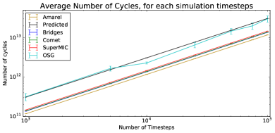
Figure 1: Average number of cycles measured on Amarel, Bridges, Comet, SuperMIC, OSG, as well as the average predicted number of cycles

Fig. 2 shows the instruction rate (i.e., the number of instructions executed per cycle) for simulations executed on the target machines, and allows us to predict the number of cycles needed to run the task on those machines.

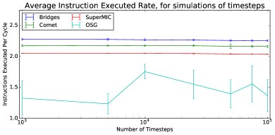
Figure 2: Instruction Rate (Instructions executed per cycle) of GROMACS simulations running on Bridges, Comet, SuperMIC and OSG

Fig. 3 shows that our model overpredicts the actual number of cycles needed to execute the simulations on XSEDE HPC machines by about 110–125%. This is unsurprising because our model does not take into account the code structure of the GROMACS simulation and the hardware architecture of the the target machines. By calculating $p2a\_cy$ for each simulation, we find that the average $\varepsilon$ for the simulations on each XSEDE HPC is less than 3%. This means that our model overpredicts because we do not consider information that describes the instruction-level parallelism which the code exploits in the hardware. We also see that our model provides more reasonable predictions of the number of cycles needed to execute simulations on OSG. However, this is most likely because we underpredicted the number of instructions required to execute a GROMACS simulation on OSG.

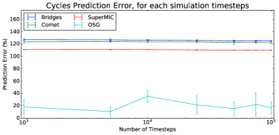
Figure 3: Prediction error of the number of cycles required to run GROMACS simulations on Bridges, Comet, SuperMIC and OSG

Fig. 4 and 5 show that our model overpredicts the task’s execution time on XSEDE HPC machines by 157–171% when using $base$ and by 84–111% when using $max$. It is important to note that using $max$ is more accurate because our model overpredicts the number of cycles required: Using faster clock frequencies masks the error introduced by overprediction.

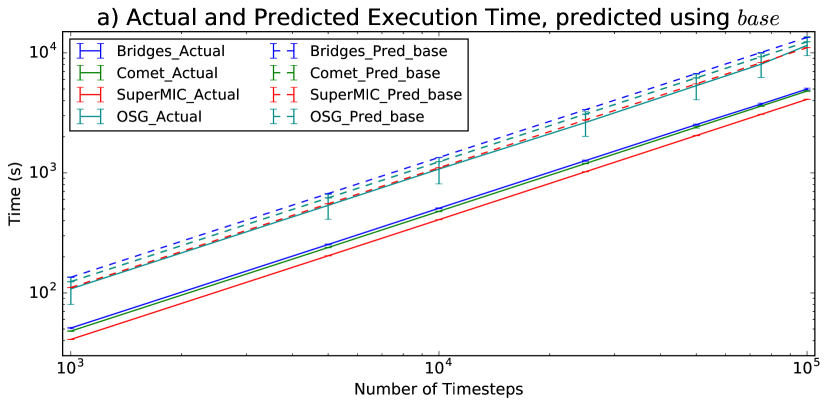
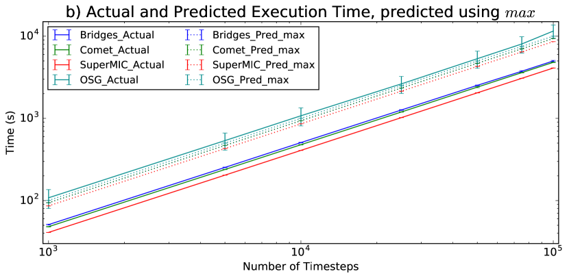
Figure 4: Average actual execution time and predicted execution times (using $base$ and $max$ frequencies) of GROMACS simulations running on Bridges, Comet, SuperMIC and OSG.

Table I shows that values of $avg$ measured on Bridges and Comet are closer to $base$ than to $max$. We also find that our model overpredicts the task’s execution time on OSG by 7–18% when using $base$ and underpredicts by 4–14% when using $max$.

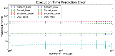
Figure 5: Prediction errors of the predicted execution times (using $base$ and $max$ frequencies) of GROMACS simulations running on Bridges, Comet, SuperMIC and OSG

Despite our model’s tendency to overpredict a task’s $T_{x}$, we can still use this model to select resource(s) if for a task $t$ and any two resources $A$ and $B$, both the actual and predicted $T_{x}$ of $t$ executed on $A$ is less than the actual and predicted $T_{x}$ of $t$ executed on $B$.

Fig. 4 shows that our model satisfies the above property when using $base$ to predict $T_{x}$ on the XSEDE HPC machines, but not when using $max$. When using the $max$ to predict $T_{x}$, the predicted $T_{x}$ for both Comet and Bridges are the same because the $max$ are the same. However, the actual $T_{x}$ measured on Comet is less than that on Bridges because $avg$ measured frequency on Comet is less than that on Bridges.

When using $base$ to predict $T_{x}$ on XSEDE HPC machines and OSG, we find that our model is inconsistent because the predicted $T_{x}$ on OSG is equal to that on Comet and less than that on Bridges; however, the actual $T_{x}$ on OSG is greater than that on both Comet and Bridges. This is because $\sim$22–24% more instructions are executed on OSG when running the same task. To enable a more direct comparison, we increased our prediction on the number of cycles on OSG by 22% to account for the additional number of executed instructions. Doing so makes the $T_{x}$ predictions generated using $base$ consistent across HPC machines and OSG.

IV-B Resource Selection

We performed a set of experiments comparing the cost of performing resource selection on the basis of our model’s predictions to the cost of a random resource selection. We expressed the cost of resource selection in terms of time-to-completion of the workload and we executed a bag-of-task workload on XSEDE HPC machines (Bridges, Comet, SuperMIC) and on OSG. Again, we call the XSEDE HPC machines and OSG as the target machines. Each task of the workload consisted of a GROMACS simulation running for $10^{5}$ timesteps as specified in Sec. IV-A.

The metric of performance used by the model is the time-to-completion of the task $TTC_{task}$: resources selected on the base of our model have the smallest predicted $TTC_{task}$. We define $TTC_{task}=T_{q,task}+T_{x,task}$, where $T_{q,task}$ and $T_{x,task}$ are the time taken to acquire the resources necessary to execute a task and the time taken to execute the task on the acquired resources, respectively.

Though any measure of cost can be used to decide how to select resources, workload’s time-to-completion is one of particular interest to users. We define the time-to-completion of a workload $TTC_{wkd}$ as $T_{q,wkd}+T_{x,wkd}$, where $T_{q,wkd,act}$ is the amount of time spent acquiring resources and $T_{x,wkd}$ is the amount of time spent executing at least one task. Using $TTC_{wkd}$ allows to measure how selecting resources that minimize the time-to-completion of each task affects the time-to-completion of the entire workload. Since time components of a task’s execution time are $T_{q,task}$ and $T_{x,task}$ and no data movement or preprocessing and post processing occurs, $TTC_{wkd}$ only involves $T_{q,wkd}$ and $T_{x,wkd}$.

IV-B1 Experimental Setup

We executed workloads with 64, 128, 256, 512, and 1024 tasks across the target machines, repeatedly over the course of a month. Only one distributed execution of the workload occurred at any given time, preventing self-competition for resource acquisition. We used RADICAL-Pilot (RP) [32] to concurrently acquire resources across the target machines and to distribute the execution of the workload across those resources.

We submitted at most one pilot [33] to the local resource manager of any XSEDE HPC machine to acquire the resources (e.g., cores and walltime) necessary to execute the entire workload. Concurrently submitting multiple pilots to the same HPC machine would have created self-competition for resources, requiring further investigation of the effects of pilot sizing on the distributed execution of the workload [34]. On OSG, we submitted only single-core pilots, enough to acquire the number of cores required to execute the entire workload. While it is possible to submit multi-core pilots to OSG, the XSEDE OSG documentation recommends against it.

When acquiring cores from XSEDE HPC machines, their resource managers return the smallest number of nodes with the number of cores requested. If the number of tasks assigned to run on an HPC machine is not a multiple of the number of cores per node, some tasks execute on a node with unused cores. We found that on SuperMIC, the $T_{x}$ of our GROMACS simulations varies up to $\sim$(19%), depending on whether all the cores of a node are utilized. To control this fluctuation in $T_{x}$ we used additional “padding tasks” to occupy all the cores of each compute node.

We used our cost model of task execution to predict $T_{x,task}$ and therefore derive $TTC_{task}$. For the values of $T_{x,task}$, we used the predictions of the execution time of a simulation running on the resources of the target machines derived using $base$ frequencies. Note that we found in Sec. IV-A that a simulation running a fixed number of timesteps performs $\sim$22–24% more instructions when executed on OSG than when executed on XSEDE HPC machines. Accordingly, we increased the predicted number of cycles required to execute a simulation on OSG by $\sim$20%.

We used XDMoD [35] to collect historical information about queue waiting times of jobs submitted to the XSEDE HPC machines to derive values for $T_{q,task}$. Since XDMoD does not provide any historical data on the queue waiting times of jobs submitted to OSG, we used a sample of trial runs for jobs submitted to OSG to calculate $T_{q,task}$. XDMoD allows us to filter historical data of queue waiting times of jobs based on the queue and machine to which the jobs were submitted, as well as the walltime and the number of cores requested.

We calculated values for the $T_{q,task}$ of a task as the average queue waiting time of jobs submitted to the same queue of the same machine that requested a ‘similar’ walltime and number of cores within the past 7 days. When filtering data on XDMoD based on requested job walltime or requested number of cores, XDMoD automatically clusters the data points into predefined ranges and limits the granularity with which we filter data. Thus, we consider two jobs to have similar requested job walltime or requested number of cores when the values of the requested job walltime (or number of cores) fall within the same predefined range. We find that for jobs requesting a large number of cores (e.g. 512, 1024 cores), there is often missing data because no jobs of that size were submitted. In this case, we used data points from jobs that were submitted to the same machine and queue.

IV-B2 Results

Fig. 6 shows the average $TTC_{wkd}$, $T_{q,wkd}$ and $T_{x,wkd}$ of the runs we performed over a month. We call the set of runs where the workload was distributed randomly the ‘baseline’ runs, and the set of runs where the workload was distributed using the cost model the ‘model’ runs. The error bars denote the sample standard deviation. During the period in which we executed the workload using our model, the target machine selected by our model using $TTC_{task}$ was SuperMIC because values of $T_{q,task}$ and $T_{w,task}$ were consistently lower than those of all the other target machines.

Fig. 6(a) shows that the average $TTC_{wkd}$ measured when distributing a workload across target machine(s) selected either randomly or using our cost model. From Fig. 6(a), we see that the average $TTC_{wkd}$ of executing a workload when the workload was distributed using our model is 67–85% lower than when executing the same workload when the workload was distributed randomly. It is important to note that the values of $T_{x,task}$ from the predictions of $T_{x}$ were generated using the $base$ frequencies of the target machines. These predictions overpredicted the actual $T_{x}$ by 157–171% (shown in Fig.  5). This shows that even inaccurate predictions of task execution time can be consistently used to select resources that support a lower workload time-to-completion than that obtained with a random resource selection.

Fig. 6(b) shows the average $T_{q,wkd}$ of the baseline and model runs. From Fig. 6(b), we see that the average $T_{q,wkd}$ and the sample standard deviation measured by the models runs are smaller than those measured by the baseline runs. This is due to the different queue waiting time across machines and the delay it introduces for task execution. Tasks randomly distributed across multiple machines waiting longer to execute than tasks submitted only to SuperMIC on the base of our model’s predictions. Consistently with other predictions and the historical data of XDMoD, during the month of our experimental campaign, SuperMIC’s queue waiting time were on average much lower and more stable than that measured on Bridges and Comet. This explains the comparatively smaller average $T_{q,wkd}$ and standard deviation of the model runs.

Note that the $T_{q,wkd}$ measured from the baseline runs is sensitive the the size of the requested resources. Queue waiting time for runs with 512 tasks/cores was consistently longer on Comet and Bridges than on SuperMIC. Further, runs with 128 tasks/cores had consistently much lower queue waiting time on all the three HPC machines. These differences may account for the variations of the sample standard deviation of $T_{q,wkd}$ in the baseline runs. Additional experiments are required to confirm the relationship between the sample standard deviation of $T_{q,wkd}$ and workload size.

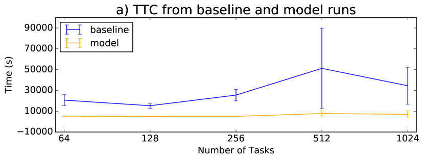
(a) $TTC_{wkd}$

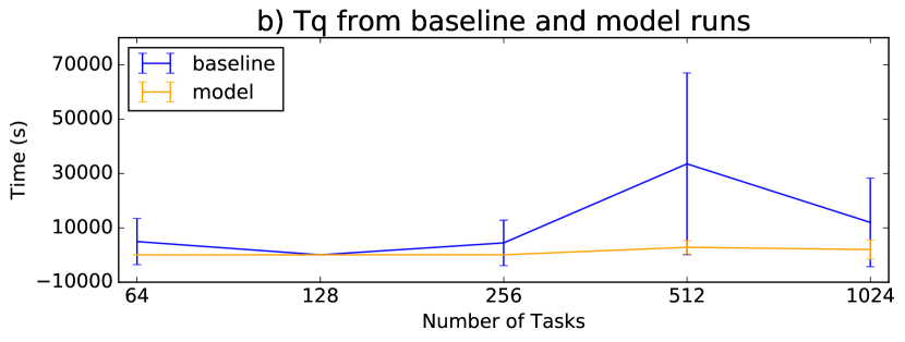
(b) $T_{q,wkd}$

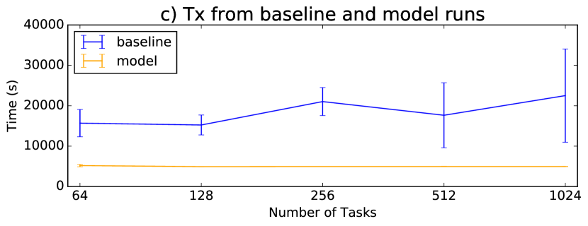
(c) $T_{x,wkd}$

Figure 6: $TTC_{wkd}$, $T_{q,wkd}$ and $T_{x,wkd}$ measured from the baseline runs and model runs.

Fig. 6(c) shows average $T_{x,wkd}$ and sample standard deviations measured by the baseline and model runs. For the model runs, we find that the values of $T_{x,wkd}$ for each workload size are almost identical, and that the sample standard deviation is negligible. Again, this is because all tasks were assigned to execute on SuperMIC. We find that the $T_{x,wkd}$ and larger sample standard deviations are higher measured from the baseline runs are higher than those measured from the model runs. One reason for this is that workloads that are distributed randomly assigned tasks to run on OSG. Tasks running on OSG have a larger execution time than when they run on any other target machine. Since OSG is a collection of resources, the execution time of the task running on an OSG resource can vary.

The second reason is that $T_{x,wkd}$ measures the amount of time where at least one task of the workload is executing. We find that the queue waiting time of pilots are staggered in time. For the baseline runs, it is common to find little or no time overlap between the execution of tasks that have been assigned to run on different DCRs. For the model runs, we make submit only one pilot to SuperMIC to acquire resources to execute the entire workload. When the pilot becomes active, all tasks in the workload execute concurrently. It is important to note this is true because we are considering homogeneous tasks. When considering homogeneous tasks, assigned all tasks to execute on one machine.

V Discussions & Conclusions

In this paper, we present a model that can predict the cost of executing a task on a resource. The model does not require information like code structure or hardware architecture. Although this limits the accuracy of its predictions, it enables the prediction of task execution times on new target resources using historical data collected on a baseline resource. Currently, the model does not take into account any parallelism which a task exploits during its execution. Extending the model to represent tasks using multithreading or multiprocessing is considered future work.

Experimental results show that the model consistently over-predicts the actual execution time of a GROMACS MD simulation running one thread and process by 157–171%. Nonetheless, the predictions can still be used to determine which resource yields the smallest execution time.

We incorporated the model into the Condor matchmaking algorithm to address the resource selection problem. The Condor matchmaking algorithm is used primarily in resource brokers to determine whether a job can run on a given resource. By adapted the matchmaking algorithm with our model, we can use the algorithm to determine which resource to use to execute a task.

We used task execution cost model and the adapted matchmaking algorithm to distribute a bag-of-task workload of GROMACS MD simulations across both HPC and HTC resources based on the expected time-to-completion of each task of the workload. For workloads of up to 1024 GROMACS simulations, our results show a reduction in the time-to-completion by 67–85% compared to randomly distributing the workload across the same resources. This shows that inaccurate predictions of execution times can still be used to select resources better than random. Moreover, it is possible to select resources where we have no historical data better than random.

Our results demonstrate the usefulness of our approach on XSEDE, but they are not limited to traditional distributed resource. For example, our resource selection models could be used to select heterogeneous virtual machine “instances” from federated cloud resources and metrics such as (fiscal) costs of instances. These extensions will be useful as the WLCG moves to incorportate cloud resources and spot markets into their mix of resources (HEPCloud [36]).

References

- [1] A. Calatrava, V. Hern et al., “Combining grid and cloud resources for hybrid scientific computing executions,” in Cloud Computing Technology and Science (CloudCom), 2011 IEEE Third International Conference on. IEEE, 2011, pp. 494–501.
- [2] E. Deelman, “Grids and clouds: Making workflow applications work in heterogeneous distributed environments,” The International Journal of High Performance Computing Applications, vol. 24, no. 3, pp. 284–298, 2010.
- [3] R. Raman, M. Livny, and M. Solomon, “Matchmaking: Distributed resource management for high throughput computing,” in High Performance Distributed Computing, 1998. Proceedings. The Seventh International Symposium on. IEEE, 1998, pp. 140–146.
- [4] T. Hoefler and R. Belli, “Scientific benchmarking of parallel computing systems: Twelve ways to tell the masses when reporting performance results,” in Proceedings of the International Conference for High Performance Computing, Networking, Storage and Analysis, ser. SC ’15. New York, NY, USA: ACM, 2015, pp. 73:1–73:12. [Online]. Available: http://doi.acm.org/10.1145/2807591.2807644
- [5] A. C. Zhou, B. He, and C. Liu, “Monetary cost optimizations for hosting workflow-as-a-service in iaas clouds,” IEEE Transactions on Cloud Computing, vol. 4, no. 1, pp. 34–48, 2016.
- [6] M. A. Rodriguez and R. Buyya, “Scheduling dynamic workloads in multi-tenant scientific workflow as a service platforms,” Future Generation Computer Systems, 2017.
- [7] G. Juve, M. Rynge, E. Deelman, J.-S. Vockler, and G. B. Berriman, “Comparing futuregrid, amazon ec2, and open science grid for scientific workflows,” Computing in Science & Engineering, vol. 15, no. 4, pp. 20–29, 2013.
- [8] E. Hwang, S. Kim, J.-S. Kim, S. Hwang, and Y.-r. Choi, “On the role of application and resource characterizations in heterogeneous distributed computing systems,” Cluster Computing, vol. 19, no. 4, pp. 2225–2240, 2016.
- [9] H. Hussain, S. U. R. Malik, A. Hameed, S. U. Khan, G. Bickler, N. Min-Allah, M. B. Qureshi, L. Zhang, W. Yongji, N. Ghani et al., “A survey on resource allocation in high performance distributed computing systems,” Parallel Computing, vol. 39, no. 11, pp. 709–736, 2013.
- [10] O. J. Workgroup, “Job submission description language (jsdl) specification, version 1.0.”
- [11] M. Solomon, “The classad language reference manual, version 2.1,” Computer Sciences Department, University of Wisconsin, Madison, WI, USA, 2003.
- [12] T. Banks, “Web services resource framework (wsrf)-primer v1. 2,” OASIS committee draft, pp. 02–23, 2006.
- [13] “Globus resource specification language.” [Online]. Available: http://toolkit.globus.org/toolkit/docs/2.4/gram/rsl_spec1.html
- [14] L. Field, C. G. Galang, and A. B. Konya, “Glue specification v. 2.0,” Recomendation GFD, vol. 147, 2009.
- [15] K. Czajkowski, S. Fitzgerald, I. Foster, and C. Kesselman, “Grid information services for distributed resource sharing,” in High Performance Distributed Computing, 2001. Proceedings. 10th IEEE International Symposium on. IEEE, 2001, pp. 181–194.
- [16] R. Wolski, N. T. Spring, and J. Hayes, “The network weather service: A distributed resource performance forecasting service for metacomputing,” Future Generation Computer Systems, vol. 15, no. 5, pp. 757–768, 1999.
- [17] R. Raman and M. Livny, “Matchmaking frameworks for distributed resource management,” University of Wisconsin-Maddison, 2001.
- [18] J. Frey, T. Tannenbaum, M. Livny, I. Foster, and S. Tuecke, “Condor-g: A computation management agent for multi-institutional grids,” in High Performance Distributed Computing, 2001. Proceedings. 10th IEEE International Symposium on. IEEE, 2001, pp. 55–63.
- [19] E. Elmroth and J. Tordsson, “A grid resource broker supporting advance reservations and benchmark-based resource selection,” in International Workshop on Applied Parallel Computing. Springer, 2004, pp. 1061–1070.
- [20] Y.-S. Kim, J.-L. Yu, J.-G. Hahm, J.-S. Kim, and J.-W. Lee, “Design and implementation of an ogsi-compliant grid broker service,” in Cluster Computing and the Grid, 2004. CCGrid 2004. IEEE International Symposium on. IEEE, 2004, pp. 754–761.
- [21] R. Buyya, D. Abramson, and J. Giddy, “Nimrod/g: An architecture for a resource management and scheduling system in a global computational grid,” in High Performance Computing in the Asia-Pacific Region, 2000. Proceedings. The Fourth International Conference/Exhibition on, vol. 1. IEEE, 2000, pp. 283–289.
- [22] A. Clematis, A. Corana, D. D’Agostino, A. Galizia, and A. Quarati, “Job–resource matchmaking on grid through two-level benchmarking,” Future Generation Computer Systems, vol. 26, no. 8, pp. 1165–1179, 2010.
- [23] R. Wilhelm, J. Engblom, A. Ermedahl, N. Holsti, S. Thesing, D. Whalley, G. Bernat, C. Ferdinand, R. Heckmann, T. Mitra et al., “The worst-case execution-time problem—overview of methods and survey of tools,” ACM Transactions on Embedded Computing Systems (TECS), vol. 7, no. 3, p. 36, 2008.
- [24] J. Abella, D. Hardy, I. Puaut, E. Quinones, and F. J. Cazorla, “On the comparison of deterministic and probabilistic wcet estimation techniques,” in Real-Time Systems (ECRTS), 2014 26th Euromicro Conference on. IEEE, 2014, pp. 266–275.
- [25] J. Abella, C. Hernandez, E. Quinones, F. J. Cazorla, P. R. Conmy, M. Azkarate-askasua, J. Perez, E. Mezzetti, and T. Vardanega, “Wcet analysis methods: Pitfalls and challenges on their trustworthiness,” in Industrial Embedded Systems (SIES), 2015 10th IEEE International Symposium on. IEEE, 2015, pp. 1–10.
- [26] F. J. Cazorla, T. Vardanega, E. Quiñones, and J. Abella, “Upper-bounding program execution time with extreme value theory,” in OASIcs-OpenAccess Series in Informatics, vol. 30. Schloss Dagstuhl-Leibniz-Zentrum fuer Informatik, 2013.
- [27] Y. Kishimoto and S. Ichikawa, “An execution-time estimation model for heterogeneous clusters,” in Parallel and Distributed Processing Symposium, 2004. Proceedings. 18th International. IEEE, 2004, p. 105.
- [28] M. A. Iverson, F. Ozguner, and L. C. Potter, “Statistical prediction of task execution times through analytic benchmarking for scheduling in a heterogeneous environment,” in Heterogeneous Computing Workshop, 1999.(HCW’99) Proceedings. Eighth. IEEE, 1999, pp. 99–111.
- [29] R. Duan, F. Nadeem, J. Wang, Y. Zhang, R. Prodan, and T. Fahringer, “A hybrid intelligent method for performance modeling and prediction of workflow activities in grids,” in Proceedings of the 2009 9th IEEE/ACM International Symposium on Cluster Computing and the Grid. IEEE Computer Society, 2009, pp. 339–347.
- [30] A. M. Chirkin, A. S. Belloum, S. V. Kovalchuk, M. X. Makkes, M. A. Melnik, A. A. Visheratin, and D. A. Nasonov, “Execution time estimation for workflow scheduling,” Future Generation Computer Systems, 2017.
- [31] 2015. [Online]. Available: https://perf.wiki.kernel.org/
- [32] A. Merzky, M. Santcroos, M. Turilli, and S. Jha, “Radical-pilot: Scalable execution of heterogeneous and dynamic workloads on supercomputers,” CoRR, vol. abs/1512.08194, 2015. [Online]. Available: http://arxiv.org/abs/1512.08194
- [33] M. Turilli, M. Santcroos, and S. Jha, “A comprehensive perspective on pilot-job systems,” arXiv preprint arXiv:1508.04180, 2015.
- [34] B. Tovar, R. F. da Silva, G. Juve, E. Deelman, W. Allcock, D. Thain, and M. Livny, “A job sizing strategy for high-throughput scientific workflows,” IEEE Transactions on Parallel and Distributed Systems, vol. PP, no. 99, pp. 1–1, 2017.
- [35] 2014. [Online]. Available: https://xdmod.ccr.buffalo.edu/
- [36] B. Holzman, L. A. T. Bauerdick, B. Bockelman, D. Dykstra, I. Fisk, S. Fuess, G. Garzoglio, M. Girone, O. Gutsche, D. Hufnagel, H. Kim, R. Kennedy, N. Magini, D. Mason, P. Spentzouris, A. Tiradani, S. Timm, and E. W. Vaandering, “Hepcloud, a new paradigm for hep facilities: Cms amazon web services investigation,” Computing and Software for Big Science, vol. 1, no. 1, p. 1, Sep 2017.