CURRENT STATUS OF WARM INFLATION

Abstract

Warm inflation is an inflationary scenario in which a thermal bath coexists with the inflaton during inflation. This is unlike standard cold inflation in which the Universe is effectively devoid of particles during inflation. The thermal bath in warm inflation is maintained by the dissipation of the inflaton’s energy through its couplings to other fields. Many models of warm inflation have been proposed and their predictions have been compared with cosmological data. Certain models of inflation that are disallowed in the context of cold inflation by the data are allowed in the warm inflationary scenario, and vice versa.

1 Introduction

In this brief article we shall provide a review of warm inflation and its current status. We shall first discuss what is warm inflation and how it is different from the standard cold inflation. We shall then discuss how to construct a warm inflation model. Finally we shall consider the compatibility of various warm inflation models with the cosmic microwave background data.

Inflation is a period of accelerated expansion in the early Universe that occurred when the Universe was $10^{-38}$ s old or later. It is invoked to solve the horizon and flatness problems. As a bonus, it provides a mechanism for generating the primordial energy density perturbations that are the seed for late time structure formation (which starts at $t\sim$ 70,000 years. During inflation the energy density of the Universe is dominated by the potential energy of a slowly moving scalar field $\phi$ called the inflaton. In Fig. 1 we see a cartoon of the inflaton potential. For $\phi<\phi_{e}$ the potential is flat and the field rolls slowly. For $\phi>\phi_{e}$ the field oscillates in its potential and decays.

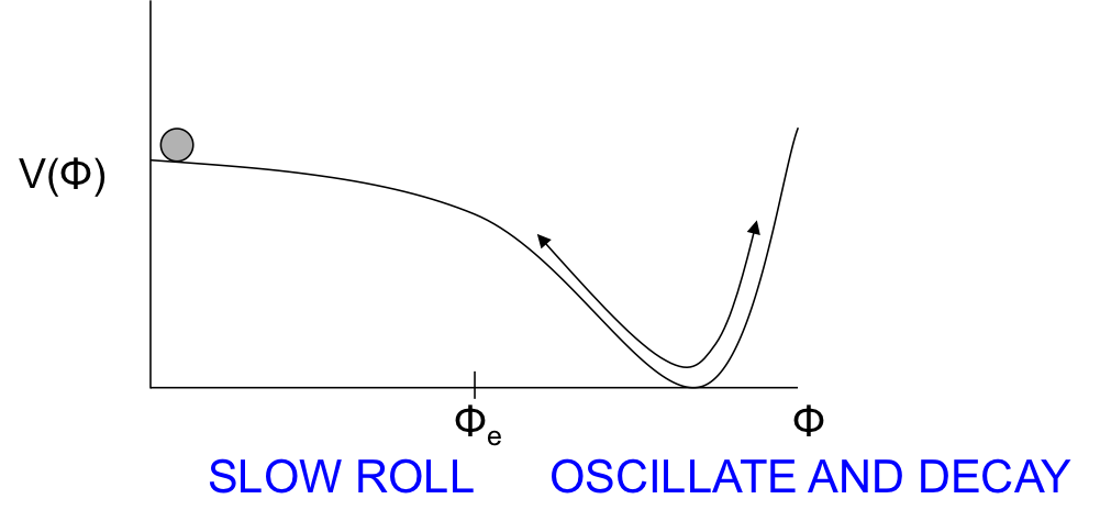
Figure 1: A cartoon of the inflaton potential.

In an expanding Universe the scale factor $a(t)$ indicates how the physical distance $d$ between points in space scales with time, $d(t)\propto a(t)$. During inflation $a$ increases as $\exp(Ht)$, where $H$ is the Hubble parameter during inflation. $Ht$ increases by a factor of at least 60 (for GUT scale inflation) and so any finite volume in the Universe increases by a factor of $\exp(180)$. (An increase in the scale factor by $e^{N}$ is referred to as there being $N$ e-foldings of inflation.) Therefore the number density of any species goes to practically 0 leaving the Universe in a supercooled state. After the inflationary era is over the inflaton decays, its decay products thermalise, and one finally has a thermal bath of quarks, leptons, gauge bosons, higgses, dark matter particles and other Beyond the Standard Model particles. This latter phase is called the reheating era. A key issue in cold inflation described above is that one ignores any decay of the inflaton during inflation.

In the warm inflation scenario the Universe inflates as in cold inflation. However one considers the decay of the inflaton during inflation. Hence the number density of particles does not go to 0 during inflation. If the dissipation is fast enough so as to maintain a thermal bath with $T>H$ then one has a warm inflation scenario $\!{{\bf??},{\bf??}}$. In some warm inflation models there is no need of a separate reheating era.

There are several models of inflation - over 70 single field inflation models are listed in Encylopedia Inflationaris $\!{{\bf??}}$. So why should one consider a new scenario like warm inflation? Firstly, it is natural to consider the effects of the inflaton couplings not just during reheating but also during inflation. (Whether or not one will get a sufficiently hot thermal bath is a different matter, as we shall see.). Furthermore, for some warm inflation models, the eta problem, namely, the presence of large quantum corrections to the inflaton potential that ruins its flatness, is resolved. Also, some potentials that are excluded by cosmic microwave background (CMB) data in the cold inflation scenario are allowed in the warm inflation scenario (though the converse is also true).

2 How is Warm Inflation Different from Cold Inflation?

It may be noted that warm inflation constitutes a different paradigm of inflation. The presence of a thermal bath differentiates it from the cold inflation scenario. While studying inflation one considers the homogeneous background field $\phi(t)$ and its spatial perturbations $\delta\phi({\bf{x}},t)$, or their Fourier transform, $\delta\phi_{k}(t)$. Both the background field and the perturbations are affected by the presence of the thermal bath.

We first consider the homogeneous inflaton field $\phi(t)$. The equation of motion of this background field is given by

$$\ddot{\phi}+(3H+\Gamma)\dot{\phi}+\frac{dV}{d\phi}=0\,,$$ (1)

where $\Gamma$ is a dissipation coefficient due to inflaton couplings to other fields, which is not considered in cold inflation during the inflaton slow roll phase. When $\Gamma>H$ it helps to slow down the inflaton. The slow roll parameters for warm inflation are given by

$$\epsilon=\frac{M_{Pl}^{2}}{16\pi}\,\left(\frac{V_{\phi}}{V}\right)^{2},\quad\eta=\frac{M_{Pl}^{2}}{8\pi}\,\frac{V_{\phi\phi}}{V},\quad\beta=\frac{M_{Pl}^{2}}{8\pi}\,\left(\frac{\Gamma_{\phi}\,V_{\phi}}{\Gamma\,V}\right)\,$$ (2)

where $M_{Pl}=1.2\times 10^{19}$ GeV is the Planck mass. The slow roll conditions needed for the inflationary phase are

$$\epsilon\ll 1+Q,\quad|\eta|\ll 1+Q,\quad|\beta|\ll 1+Q\,,$$ (3)

where $Q=\Gamma/(3H)$. The presence of Q on the right hand side, which is obviously absent in cold inflation, implies that the slow roll conditions can be satisfied even if the slow roll parameters are large, if $Q\gg 1$, as it happens in some models of warm inflation. In these models of warm inflation, the eta problem is solved. Finally in some models of warm inflation, before the slow roll conditions break down the inflaton energy density becomes smaller than the radiation energy density. In that case inflation ends but then there is no separate reheating phase because one has an automatic transition to the radiation dominated era (though the inflaton will eventually oscillate and decay).

The thermal bath affects the inflaton perturbations and thereby the primordial curvature perturbations. The curvature perturbations affect the CMB anisotropy and the large scale structure that we observe today. The equation of motion for the inflation perturbations in the presence of the thermal bath is given by $\!{{\bf??},{\bf??},{\bf??}}$

$$\delta\ddot{\phi}_{k}+(3H+\Gamma)\,\delta\dot{\phi}_{k}+\left(\frac{k^{2}}{a^{2}}+V_{\phi\phi}\right)\delta\phi_{k}=\sqrt{2\,\Gamma\,T}\,a^{-3/2}\,\xi_{k}\,,$$ (4)

where $\xi_{k}$ represents thermal noise. The above is a form of the Langevin equation with the fluctuation term on the r.h.s. related to the dissipation term on the l.h.s. The primordial curvature power spectrum is proportional to $|\delta\phi_{k}|^{2}$ (in the spatially flat gauge), where $\delta\phi_{k}$ is evaluated when the physical wavelength of the perturbation $(\lambda_{phys}=2\pi a(t)/k)$ becomes large enough that $\delta\phi_{k}$ becomes constant, or freezes out $\!{{\bf??}}$.

We are concerned only with the perturbations that correspond to cosmologically relevant length scales today, from $10^{-3}$ Mpc to 14000 Mpc $\!{{\bf??}}$. This corresponds to about 16 e-foldings of inflation, starting from about 60 e-foldings of inflation before the end of inflation (for GUT scale inflation). The observed CMB anisotropy reflects perturbations on scales of 10 Mpc and larger. When $Q\ll 1\,(Q\gg 1)$ it is referred to as weak (strong) dissipative warm inflation. The inflaton perturbations for cold inflation, weak dissipative warm inflation and strong dissipative warm inflation are given by $\!{{\bf??},{\bf??}}$

$$\delta\phi_{k} \sim H$$ Cold Inflation

$$\delta\phi_{k} \sim\sqrt{HT}$$ Weak Dissipative Warm Inflation

$$\delta\phi_{k} \sim\sqrt{T(H\Gamma)^{\frac{1}{2}}}$$ Strong Dissipative Warm Inflation (5)

The primordial curvature power spectrum (or scalar power spectrum) is given in Ref. $\!{{\bf??}}$ (based on Refs. $\!{{\bf??},{\bf??},{\bf??},{\bf??},{\bf??}}$) as

$$P_{\mathcal{R}}(k)=\left({H_{k}\over\dot{\phi}_{k}}\right)^{2}\left({H_{k}\over 2\pi}\right)^{2}\left[1+2n_{k}+\left(T_{k}\over H_{k}\right){2\sqrt{3}\pi Q_{k}\over\sqrt{3+4\pi Q_{k}}}\right]~{},$$ (6)

where the subscript $k$ indicates that the variable is evaluated at the time of horizon crossing of the $k$ mode perturbation $\delta\phi_{k}$, and $n_{k}$ represents the distribution of inflaton particles in the thermal bath. In the literature, one considers either $n_{k}=0$ or the Bose-Einstein distribution, $n(k)=[\exp\{k/(aT)\}-1]^{-1}$. For the latter case, $1+2n_{k}=\coth[H_{k}/(2T_{k})]$, using $k/a_{k}=H_{k}$. In addition to the explicit temperature dependence in the square bracket above, the prefactor (whose form is the same as that for cold inflation) will reflect the influence of dissipation. Note that $[H_{k}/(2\pi)]^{2}$ times the first term in the square bracket reflects the standard quantum contribution, as in cold inflation, its product with $\coth[H_{k}/(2T_{k})]$ reflects the weak dissipative warm inflation result for $T\gg H$, and the product with the last term indicates the strong dissipative warm inflation result, as in Eq. (5).

Inflation gives rise to both scalar and tensor perturbations of the metric. Gravitational waves are weakly coupled to the thermal bath and so the tensor power spectrum has the same form as in cold inflation, namely,

$$P_{T}(k)=\frac{16}{\pi}\frac{H_{k}^{2}}{M_{Pl}^{2}}\,.$$ (7)

The tensor-to-scalar ratio $r$ is defined, as usual, as

$$r=\frac{P_{T}(k_{P})}{P_{\mathcal{R}}(k_{P})}$$ (8)

where $k_{P}$ refers to the pivot scale, a fiducial scale for which there is greater observational accuracy for any particular experiment.

3 Constructing a Warm Inflation Model

The dissipation coefficient $\Gamma$ reflects the transfer of energy from the inflaton field to the thermal bath. If one couples the radiation, i.e. light fields with mass $m<T$, directly to the inflaton then one gets a $\Gamma\dot{\phi}$ term in the equation of motion for $\phi$ but one also gets large thermal corrections to the inflaton potential and too few e-foldings of inflation $\!{{\bf??},{\bf??}}$. There are two approaches to avoiding this. In the first approach one couples the inflaton only to heavy fields through a superpotential of the form $\!{{\bf??}}$

$$W=f(\Phi)+{g\over 2}\Phi X^{2}+{h\over 2}XY^{2}~{},$$ (9)

where $\phi$ is associated with the scalar component of the $\Phi$ superfield, and the $X$ fields are heavy, i.e $m_{X}>T$, while the $Y$ fields are light $(m_{Y}<T)$. The inflaton field can decay to $Y$ particles either through virtual $X$ when $T\ll m_{X}$, or through decay to real $X$ which then decay to $Y$ when $T<m_{X}$ and $h\sqrt{N_{Y}}$ is small $\!{{\bf??}}$. The form of the dissipation coefficient is $\Gamma=C_{\phi}T^{3}/\phi^{2}$. The heavy $X$ ensure that the thermal corrections are small and supersymmetry ensures that the vacuum corrections are small. However, viable models of warm inflation need $10^{6}$ or $10^{4}$ $X$ fields to satisfy warm inflation requirements, particularly $T>H$ during inflation $\!{{\bf??},{\bf??}}$. Such a large number of fields are obtained by considering brane-antibrane models of inflation where the $X$ fields correspond to strings stretched between brane and antibrane stacks $\!{{\bf??}}$, or extra-dimensional scenarios with a tower of Kaluza-Klein modes $\!{{\bf??}}$.

In the second approach to constructing a warm inflation model, one makes the inflaton field a pseudo-Nambu-Goldstone boson. This has been realised in warm natural inflation models $\!{{\bf??}}$, and the warm little inflation model (which is similar to the little Higgs model) $\!{{\bf??}}$. In these models it is sufficient for the inflaton to couple to a few fields. In Ref. $\!{{\bf??}}$, there is one additional pseudo-Nambu Goldstone boson besides the inflaton and another light field, and $\Gamma\sim\dot{\phi}^{2}T$ and $Q\gg 1$. In Ref. $\!{{\bf??}}$ the inflaton field is coupled to two light fields, and $\Gamma=C_{T}T$ and both weak and strong dissipative warm inflation scenarios are considered.

4 Comparing with Data

Various models of warm inflation, as identified by the inflaton potential and the form of the dissipation coefficient, have been studied and compared with the cosmological data. $\Upsilon=C_{\phi}T^{3}/\phi^{2}$ and $\Gamma=C_{T}T$ are the usual forms of the dissipation coefficient considered in the literature. In general, $\Gamma=C_{\phi}T^{c}\phi^{2a}/M_{X}^{2b}$ with $c+2a-2b=1$ $\!{{\bf??}}$.

Limits from cosmological data are often written in terms of allowed values of the spectral index $n_{s}$ defined as $n_{s}-1=d\ln P_{\mathcal{R}}/d\ln k|_{k_{P}}$ and the tensor-to-scalar ratio $r$. In Fig. 2 one sees the region in the $r-n_{s}$ plane allowed by WMAP in teal $\!{{\bf??},{\bf??}}$. Also plotted are the $r-n_{s}$ values obtained for warm inflation models with monomial potentials $(V\sim\phi^{n})$ as separate curves in the figure. $n=2,4$ and 6 are considered, for two values of the number of e-foldings of inflation from when the perturbation associated with the pivot scale crosses the horizon till the end of inflation, i.e. $N_{e}$ equal to 60 and 40. We can focus on the $N_{e}=60$ curves for warm inflation. Along each curve, the different points correspond to different values of $Q(k_{P})$ with the values increasing as one goes down the curve. The cold inflation curves (CI) are also shown. For cold inflation models the different points correspond to values of $N_{e}$ varying from 50 to 60 (from left to right).

We notice that quadratic warm inflation has too large a value of $n_{s}$ and so is disallowed, while it is consistent with the data for cold inflation. On the other hand, quartic and sextic cold inflation are ruled out by the data while they are allowed in warm inflation for appropriate values of $Q(k_{P})$.

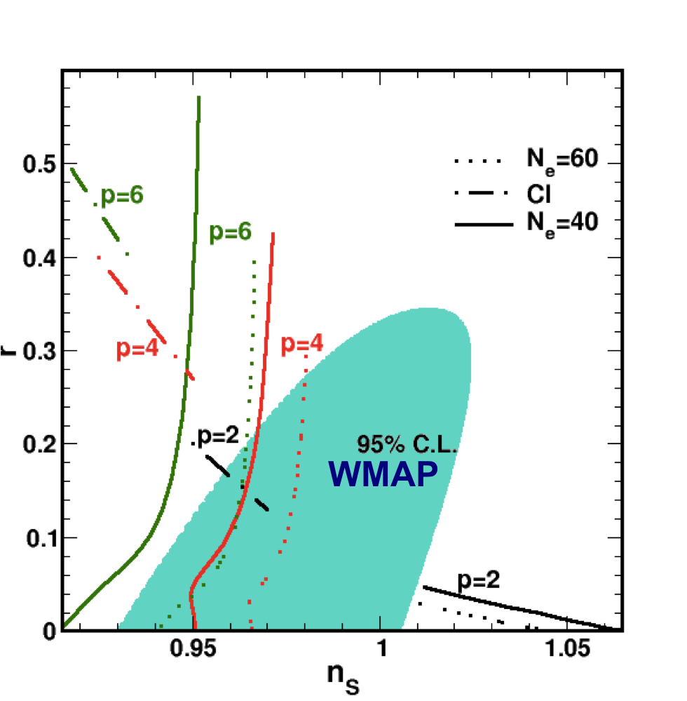
Figure 2: Allowed region by WMAP in $r-n_{s}$ plane is shown in teal. Also plotted are the $r-n_{s}$ values obtained for quadratic, quartic and sextic warm inflation models (solid and dotted lines) for $N_{e}$=40 and 60, and cold inflation models (dot-dash) for varying $N_{e}$.

In Ref. $\!{{\bf??}}$ the authors perform a Markov Chain Monte Carlo analysis of the parameters of warm inflation using the publicly available CosmoMC programme $\!{{\bf??}}$ and the Planck data. They perform this analysis for quartic, sextic, hilltop, Higgs and plateau sextic warm inflation models for $\Gamma\propto T^{3}$ and $T$ and find parameters compatible with the Planck data for $Q(k_{P})$ between $10^{-3}$ and 1.4 and $r$ between $10^{-9}$ and 0.036 for different models. Another CosmoMC analysis of quartic warm inflation using Planck data obtains the joint probability distribution for the inflaton self-coupling $\lambda$ and $Q(k_{P})$ for $N_{e}=50$ and 60 $\!{{\bf??}}$, as shown in Fig. 3. From the marginalised distributions of the parameters of the model the preferred range of values for $\lambda$ for $N_{e}=50$ is $1.5\times 10^{-14}$ to $1.9\times 10^{-14}$ with a mean value of $1.6\times 10^{-14}$, and the preferred range of values for $N_{e}=60$ is $9.2\times 10^{-15}$ to $1.1\times 10^{-14}$ with a mean value of $1.0\times 10^{-14}$. The preferred range of values for $Q_{P}$ is $9.5\times 10^{-4}$ to $1.4\times 10^{-2}$ with a mean value of $3.7\times 10^{-3}$ for $N_{e}=50$, and the preferred range of values for $N_{e}=60$ is $1.6\times 10^{-3}$ to $1.2\times 10^{-2}$ with a mean value of $4.4\times 10^{-3}$. Another CosmoMC analysis for a quartic inflaton potential with $\Gamma\propto T$ has been carried out in Ref. $\!{{\bf??}}$.

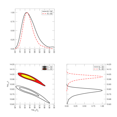
Figure 3: The joint probability distribution for the inflaton self-coupling $\lambda$ and $Q(k_{P})$ for $N_{e}=50$ and 60. The preferred range of values for $\lambda$ is $1.5\times 10^{-14}$ to $1.9\times 10^{-14}$ for $N_{e}=50$, and is $9.2\times 10^{-15}$ to $1.1\times 10^{-14}$ for $N_{e}=60$. The preferred range of values for $Q_{P}$ is $9.5\times 10^{-4}$ to $1.4\times 10^{-2}$ for $N_{e}=50$, and is $1.6\times 10^{-3}$ to $1.2\times 10^{-2}$ for $N_{e}=60$.

Warm natural inflation models too have been compared with the cosmological data. In the model studied in Ref. $\!{{\bf??}}$ it is found that warm natural inflation is viable for the scale of symmetry breaking (that creates the pseudo-Nambu-Goldstone boson) to be between the GUT scale and the Planck scale, while Ref. $\!{{\bf??}}$ finds that the symmetry breaking scale in their model should be the GUT scale. In both models what is significant is that symmetry breaking scales well below the Planck scale are allowed. Planck scale symmetry breaking was one of the less attractive features of cold natural inflation.

Ref. $\!{{\bf??}}$ shows that hybrid inflation, which involves the interplay of two fields during inflation, is consistent with the data for warm inflation, in contrast with cold inflation. The viability of brane inflation, G(alileon) inflation and non-canonical inflation has also been studied in Refs. $\!{{\bf??},{\bf??},{\bf??}}$.

5 Conclusion

In summary, warm inflation is a viable paradigm of inflation. Various warm inflation models are compatible with cosmological data. Models such as monomial quartic and sextic warm inflation and hybrid warm inflation are allowed by the data while the corresponding models in the cold inflationary scenario are disallowed by the data. On the contrary, the quadratic inflationary model is disallowed in warm inflation while consistent with the data for cold inflation. In the case of natural warm inflation the relevant energy scale can be brought down from the Planck scale, as in cold inflation, to the GUT scale. While the requirement of a large number of fields coupled to the inflaton to satisfy the conditions for warm inflation is unattractive this issue has been resolved in warm inflation models where the inflaton is a pseudo-Nambu-Goldstone boson.

There have been interesting results associated with viscosity in the thermal bath during inflation, and on the generation of non-Gaussian fluctuations during warm inflation, which have not been discussed here.

References

- [1] A. Berera and L. -Z. Fang, Phys. Rev. Lett. 74, 1912 (1995) [astro-ph/9501024].
- [2] A. Berera, Phys. Rev. Lett. 75, 3218 (1995) [astro-ph/9509049].
- [3] J. Martin, C. Ringeval and V. Vennin, Phys. Dark Univ. 5-6, 75 (2014) [arXiv:1303.3787 [astro-ph.CO]].
- [4] L. M. Hall, I. G. Moss and A. Berera, Phys. Rev. D 69, 083525 (2004) [astro-ph/0305015].
- [5] R. O. Ramos and L. A. da Silva, JCAP 1303, 032 (2013) [arXiv:1302.3544 [astro-ph.CO]].
- [6] S. Bartrum, M. Bastero-Gil, A. Berera, R. Cerezo, R. O. Ramos and J. G. Rosa, Phys. Lett. B 732, 116 (2014) [arXiv:1307.5868 [hep-ph]].
- [7] A. Berera, Nucl. Phys. B 585, 666 (2000) [hep-ph/9904409].
- [8] D. H. Lyth and A. R. Liddle, Cambridge, UK: Cambridge Univ. Press (2009) [Sec. 7.1].
- [9] A. Berera, Contemp. Phys. 47, 33 (2006) [arXiv:0809.4198 [hep-ph]].
- [10] I. G. Moss, Phys. Lett. B 154, 120 (1985).
- [11] A. Berera, M. Gleiser and R. O. Ramos, Phys. Rev. D 58, 123508 (1998) [hep-ph/9803394].
- [12] J. Yokoyama and A. D. Linde, Phys. Rev. D 60, 083509 (1999) [hep-ph/9809409].
- [13] I. G. Moss and C. Xiong, hep-ph/0603266.
- [14] M. Bastero-Gil, A. Berera, R. O. Ramos and J. G. Rosa, JCAP 1301, 016 (2013) [arXiv:1207.0445 [hep-ph]].
- [15] A. Berera, M. Gleiser and R. O. Ramos, Phys. Rev. Lett. 83, 264 (1999) [hep-ph/9809583].
- [16] M. Bastero-Gil, A. Berera and N. Kronberg, JCAP 1512, no. 12, 046 (2015) [arXiv:1509.07604 [hep-ph]].
- [17] M. Bastero-Gil, A. Berera and J. G. Rosa, Phys. Rev. D 84, 103503 (2011) [arXiv:1103.5623 [hep-th]].
- [18] T. Matsuda, Phys. Rev. D 87, 026001 (2013) [arXiv:1212.3030 [hep-th]].
- [19] H. Mishra, S. Mohanty and A. Nautiyal, Phys. Lett. B 710, 245 (2012) [arXiv:1106.3039 [hep-ph]].
- [20] M. Bastero-Gil, A. Berera, R. O. Ramos and J. G. Rosa, Phys. Rev. Lett. 117, 151301 (2016) [arXiv:1604.08838 [hep-ph]].
- [21] M. Bastero-Gil and A. Berera, Int. J. Mod. Phys. A 24, 2207 (2009) [arXiv:0902.0521 [hep-ph]].
- [22] M. Bastero-Gil, Talk at “Cosmological perturbations post-Planck”, 4-7 June 2013, Helsinki.
- [23] M. Benetti and R. O. Ramos, Phys. Rev. D 95, no. 2, 023517 (2017) [arXiv:1610.08758 [astro-ph.CO]].
- [24] A. Lewis and S. Bridle, Phys. Rev. D 66 (2002) 103511. Given a primordial power spectrum written in terms of the parameters of any inflation model, CosmoMC obtains the angular power spectrum of the CMB temperature anisotropies (’s), compares it with the angular power spectrum obtained from the data, and thereby obtains marginalised probability distributions (and the corresponding mean values and standard deviations) as well as joint probability distributions for the parameters of the inflation model (and other cosmological parameters).
- [25] R. Arya, A. Dasgupta, G. Goswami, J. Prasad and R. Rangarajan, arXiv:1710.11109 [astro-ph.CO].
- [26] M. Bastero-Gil, S. Bhattacharya, K. Dutta and M. R. Gangopadhyay, arXiv:1710.10008 [astro-ph.CO].
- [27] L. Visinelli, JCAP 1109, 013 (2011) [arXiv:1107.3523 [astro-ph.CO]].
- [28] M. Bastero-Gil, A. Berera, T. P. Metcalf and J. G. Rosa, JCAP 1403, 023 (2014) [arXiv:1312.2961 [hep-ph]].
- [29] M. A. Cid, S. del Campo and R. Herrera, JCAP 0710, 005 (2007) [arXiv:0710.3148 [astro-ph]].
- [30] S. del Campo and R. Herrera, Phys. Lett. B 653, 122 (2007) [arXiv:0708.1460 [gr-qc]].
- [31] R. Herrera, JCAP 1705, no. 05, 029 (2017) [arXiv:1701.07934 [gr-qc]].