An ALMA [C ii] survey of 27 quasars at $z>5.94$

Abstract

We present a survey of the [C ii] 158 $\mu$m line and underlying far–infrared (FIR) dust continuum emission in a sample of 27 $z\mathrel{\hbox to0.0pt{\lower 3.0pt\hbox{$\sim$}\hss}\raise 2.0pt\hbox{$>$}}6$ quasars using the Atacama Large Millimeter Array (ALMA) at $\sim 1^{\prime\prime}$ resolution. The [C ii] line was significantly detected (at $>5$-$\sigma$) in 23 sources (85%). We find typical line luminosities of $L_{\rm[CII]}=10^{9-10}$ L_⊙, and an average line width of $\sim 450$ km s^-1. The [C ii]–to–far-infrared luminosity ratio ([C ii]/FIR) in our sources span one order of magnitude, highlighting a variety of conditions in the star–forming medium. Four quasar host galaxies are clearly resolved in their [C ii] emission on a few kpc scales. Basic estimates of the dynamical masses of the host galaxies give masses between $2\times 10^{10}$ and $2\times 10^{11}$ M_⊙, i.e., more than an order of magnitude below what is expected from local scaling relations, given the available limits on the masses of the central black holes ($>3\times 10^{8}$ M_⊙, assuming Eddington-limited accretion). In stacked ALMA [C ii] spectra of individual sources in our sample, we find no evidence of a deviation from a single Gaussian profile. The quasar luminosity does not strongly correlate with either the [C ii] luminosity or equivalent width. This survey (with typical on–source integration times of 8 min) showcases the unparalleled sensitivity of ALMA at millimeter wavelengths, and offers a unique reference sample for the study of the first massive galaxies in the universe.

1 Introduction

Quasars are the most luminous, non-transient sources in the early universe, and therefore represent ideal laboratories to investigate the first stages of galaxy formation. They were among the first high–redshift ($z>1$) targets for sub-mm observations (e.g., Omont et al., 1996). Various campaigns with bolometers mounted on single-dish telescopes (e.g., Bertoldi et al., 2003a; Beelen et al., 2006; Wang et al., 2008a, b) as well as with the Herschel observatory (e.g., Leipski et al., 2014; Drouart et al., 2014) extensively sampled the far–infrared (FIR) spectral energy distributions (SEDs) of these sources. This suggested that about 1/3 of high–redshift quasars are hosted in infrared- (IR-) bright ($\sim 10^{13}$ L_⊙) host galaxies (Leipski et al., 2014). Although the rapid accretion of material onto the central supermassive black hole may be responsible for contributing to at least part of this IR luminosity (e.g., Barnett et al., 2015; Schneider et al., 2015), it is now established that the majority of this emission is powered by star formation rates (SFRs) of several hundred solar masses per year or more in the host galaxies (Walter et al., 2009; Leipski et al., 2014). These prodigious events of star formation are fueled by immense (a few times $10^{10}$ M_⊙) reservoirs of molecular gas, which can be detected through the rotational transitions of the carbon monoxide (CO) molecule (e.g., Carilli et al., 2002; Bertoldi et al., 2003b; Walter et al., 2003, 2004; Riechers et al., 2006, 2009; Wang et al., 2010; Venemans et al., 2017b). The gaseous reservoirs often appear spatially compact, with sizes of a few kpc or less (e.g., Riechers et al., 2007; Walter et al., 2009; Wang et al., 2013; Willott et al., 2013; Venemans et al., 2017a). The implied star formation rate surface densities, $\Sigma_{\rm SFR}$, can be extremely high ($\sim 1000$ M_⊙ yr^-1 kpc^-2), and might even reach the Eddington limit for star formation (Scoville, 2004; Thompson et al., 2005; Walter et al., 2009). High CO excitation is observed in some of these quasars, as would be expected in compact violent starbursts (e.g., Barvainis et al., 1997; Walter et al., 2003; Bertoldi et al., 2003a; Weiß et al., 2007; Riechers et al., 2009, 2011a).

The redshift range $z\mathrel{\hbox to0.0pt{\lower 3.0pt\hbox{$\sim$}\hss}\raise 2.0pt\hbox{$>$}}6$ (when the age of the universe is less than 1 Gyr) is of particular interest. The steep evolution of the average UV transmission due to neutral hydrogen’s Lyman $\alpha$ line points to a rapid change in the ionization properties of the intergalactic medium, suggesting that we are entering the epoch of reionization at these redshifts (Fan et al., 2006). In this early phase of galaxy formation, quasar host galaxies stand out as some of the most active regions of the universe. To date (Dec 2017), there are $\sim 225$ quasars known in the literature at $z>5.5$, 119 at $z>6.0$, 15 at $z>6.5$, and only 2 at $z>7.0$ (see, e.g., Fan et al. 2006, Mortlock et al. 2011, Venemans et al. 2013, Bañados et al. 2016, Jiang et al. 2016, Matsuoka et al. 2016, 2017, Wang et al. 2017, Mazzucchelli et al. 2017, Bañados et al. 2017, and references therein). Their black hole masses, typically estimated from the Mgii broad emission line at 2796 Å rest frame, are of the order of $10^{9}$ M_⊙ (e.g., Jiang et al., 2008; De Rosa et al., 2011, 2014). The required rapid build-up of the black holes has sharpened our understanding of how these black holes form in the first place (see Volonteri, 2012, for a review). Both the gas in the broad line region around the central black hole, and the interstellar medium (ISM) of their host galaxies appear metal–enriched (e.g., De Rosa et al., 2011; Mortlock et al., 2011; Walter et al., 2003; Bertoldi et al., 2003a, b; Beelen et al., 2006). This hints that the first generation of stars in these objects formed very rapidly.

At $z\mathrel{\hbox to0.0pt{\lower 3.0pt\hbox{$\sim$}\hss}\raise 2.0pt\hbox{$>$}}6$, the fine–structure line of singly ionized carbon, [C ii] at 158 $\mu$m (hereafter, [C ii]), conveniently enters the 1.2mm transparent atmospheric window, thus enabling it to be observed from the ground. The [C ii] line is the main coolant of the cool ($<1000$ K) ISM, in some cases reaching luminosities as high as $\sim 1$ per cent of the entire far-infrared luminosity of a galaxy (see, e.g., Díaz-Santos et al., 2017, for a recent compilation). Because of this, it plays a key role in the thermodynamical evolution of the ISM. Also, due to its high brightness and narrowness (as it traces the host galaxy, rather than the turbulent region close to the active nucleus), the [C ii] line is an excellent observational tool to measure precise redshifts. These are important, for instance, in the study of the proximity zone and in the determination of the quasar lifetime (see, e.g., Fan et al. 2006, Carilli et al. 2010, Eilers et al. 2017), and to probe the gas kinematics (thus inferring the dynamical mass of the host galaxy, or exposing the presence of outflows and winds; see, e.g., Venemans et al. 2012, 2016; Willott et al. 2013, 2015; Wang et al. 2013, 2016; Cicone et al. 2015). Because of its intimate connection with the cooling of the ISM, [C ii] can also be used as a tracer of star formation (e.g., De Looze et al., 2014; Herrera-Camus et al., 2015). Thanks to all these virtues, [C ii] has become a workhorse diagnostic line for the study of the ISM in galaxies at $z\mathrel{\hbox to0.0pt{\lower 3.0pt\hbox{$\sim$}\hss}\raise 2.0pt\hbox{$>$}}6$.

In fact, the first [C ii] line detection reported at $z>0.1$ was associated with the host galaxy of the quasar J1148+5251, at $z=6.4$ (Maiolino et al., 2005). This study, performed with the IRAM 30m single–dish telescope, demonstrated the feasibility of the observation of fine–structure lines (and, in particular, of [C ii]) in $z\mathrel{\hbox to0.0pt{\lower 3.0pt\hbox{$\sim$}\hss}\raise 2.0pt\hbox{$>$}}6$ galaxies. Later studies of $z\mathrel{\hbox to0.0pt{\lower 3.0pt\hbox{$\sim$}\hss}\raise 2.0pt\hbox{$>$}}6$ quasars targeting the [C ii] line and the underlying dust continuum capitalized on the technological improvement in sensitivity offered by the IRAM Plateau de Bure Interferometer (PdBI, now upgraded to the NOrthern Extended Millimeter Array, NOEMA; Walter et al. 2009; Venemans et al. 2012; Bañados et al. 2015; Mazzucchelli et al. 2017) and on the advent of the Atacama Large Millimeter Array (ALMA; Willott et al., 2013, 2015; Wang et al., 2013; Venemans et al., 2016). This decade–long effort by the community resulted in a sample of 18 quasars at $z\mathrel{\hbox to0.0pt{\lower 3.0pt\hbox{$\sim$}\hss}\raise 2.0pt\hbox{$>$}}6$ with [C ii] detections (at various degrees of significance).

In this paper, we mark a major step in terms of sample size. Using ALMA, we surveyed the [C ii] line and the underlying dust continuum emission in 27 $z\mathrel{\hbox to0.0pt{\lower 3.0pt\hbox{$\sim$}\hss}\raise 2.0pt\hbox{$>$}}6$ quasar host galaxies. The size of the sample and the homogeneous data quality, together with the consistent analysis, allow us for the first time to study quasar host galaxies at the end of the reionization as a population. In addition, in Decarli et al. (2017) we presented a blind search for line emission in these data cubes that resulted in the detection of [C ii]–bright galaxy companions in four of the quasars in our sample. These companion galaxies offer a first insight on the properties of the close galactic environment of $z\mathrel{\hbox to0.0pt{\lower 3.0pt\hbox{$\sim$}\hss}\raise 2.0pt\hbox{$>$}}6$ quasars. The focus of the present paper is on the line properties of the quasar host galaxies themselves, while a companion paper (Venemans et al. in prep.) will analyze the underlying continuum emission from the same dataset.

The paper is organized as follows: In Section 2 we outline our survey and the reference sample from the literature; in Section 3 we describe the observations and the data reduction; in Sections 4 and 5 we present the measurements and infer derived quantities, respectively. Finally, we discuss our results and draw our conclusions in Section 6.

Throughout the paper we assume a standard $\Lambda$CDM cosmology with $H_{0}=70$ km s^-1 Mpc^-1, $\Omega_{\rm m}=0.3$ and $\Omega_{\Lambda}=0.7$ (consistent with the measurements by the Planck Collaboration, 2015). Magnitudes are reported in the AB photometric system.

2 The [C ii] survey

2.1 The main sample

The parent sample of our ALMA survey was designed to include all the known quasars matching the following criteria:

• they lie at $z>5.94$ (i.e., $\nu_{\rm obs}$([C ii]) $<273.854$ GHz), so that the [C ii] line falls in ALMA band 6 ($\sim 1.2$mm);

• they are at declination Decl. $<+15^{\circ}$, so that they can be observed at high elevation from the ALMA site;

• they are more luminous than $M_{1450}$=$-25.25$ mag, where $M_{1450}$ is the absolute magnitude derived from broad-band imaging observations of the rest-frame FUV continuum.

• they were not previously targeted in the [C ii] line.

At the time of the ALMA Cycle 3 deadline (April 2015), there were 57 published quasars at $z>5.94$, 39 of which match the declination requirement. Two of these objects do not match the FUV luminosity requirement. Eleven of the remaining 37 sources had been observed in [C ii] in past programs, either with ALMA or other facilities (mostly, IRAM/PdBI). We also include 9 new quasars that match our selection criteria but were still unpublished at the time the proposal was submitted (Bañados et al., 2016; Mazzucchelli et al., 2017, Venemans et al. in prep.). The final sample therefore consists of 35 sources (see Table 2). Observations were performed for 27 of them, chosen only due to their visibility at the time of the observations. For reference, Figure 1 shows the redshift distribution of the quasars in our sample, compared to all the other quasars currently known in this redshift range.

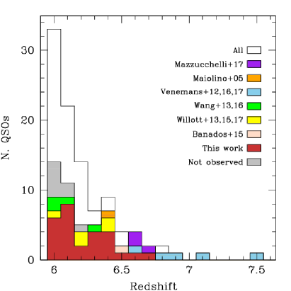
Figure 1: Redshift distribution of the quasars in our sample (observed: dark red; unobserved: grey), compared with the other $z\mathrel{\hbox to0.0pt{\lower 3.0pt\hbox{$\sim$}\hss}\raise 2.0pt\hbox{$>$}}6$ quasars with [C ii] observations (filled histograms – see the legend for references) and the parent sample of all known $z\mathrel{\hbox to0.0pt{\lower 3.0pt\hbox{$\sim$}\hss}\raise 2.0pt\hbox{$>$}}6$ quasars.

2.2 The sample from the literature

Our results are complemented with all the [C ii] and underlying dust continuum observations of $z>5.94$ quasars available in the literature. This sample consists of 1 quasar from Maiolino et al. (2005) and Walter et al. (2009); 1 quasar from Bañados et al. (2015); 5 quasars from Venemans et al. (2012, 2016, 2017a, 2017c); 5 from Willott et al. (2013, 2015, 2017); 4 quasars from Wang et al. (2013, 2016); and 3 from Mazzucchelli et al. (2017). The sample from the literature is presented in Table 3. For these sources, we will use the line luminosity and width, and the dust continuum flux density derived in the papers quoted above. For consistency with the rest of our sample, however, we re-derive the IR luminosity using the same approach adopted for the main sample of this work.

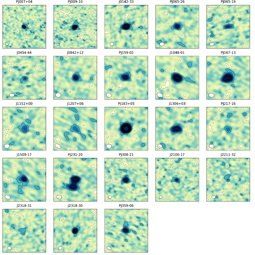
Figure 2: ALMA postage stamps showing the continuum-subtracted [C ii] line maps of each of the 27 sources in our sample, integrated over a width of $\pm 1.4\times\sigma_{\rm line}$, in order to maximize the line S/N. Each panel is $10^{\prime\prime}\times 10^{\prime\prime}$ wide. North is up, East to the left. Only quasars with a [C ii] detection are shown. The solid black / dashed blue contours mark the $\pm 2,4,6,$…$\sigma$ isophotes. The synthesized beam of the observations is shown in the bottom-left corner of each panel. Extended names are reported in Table 2.

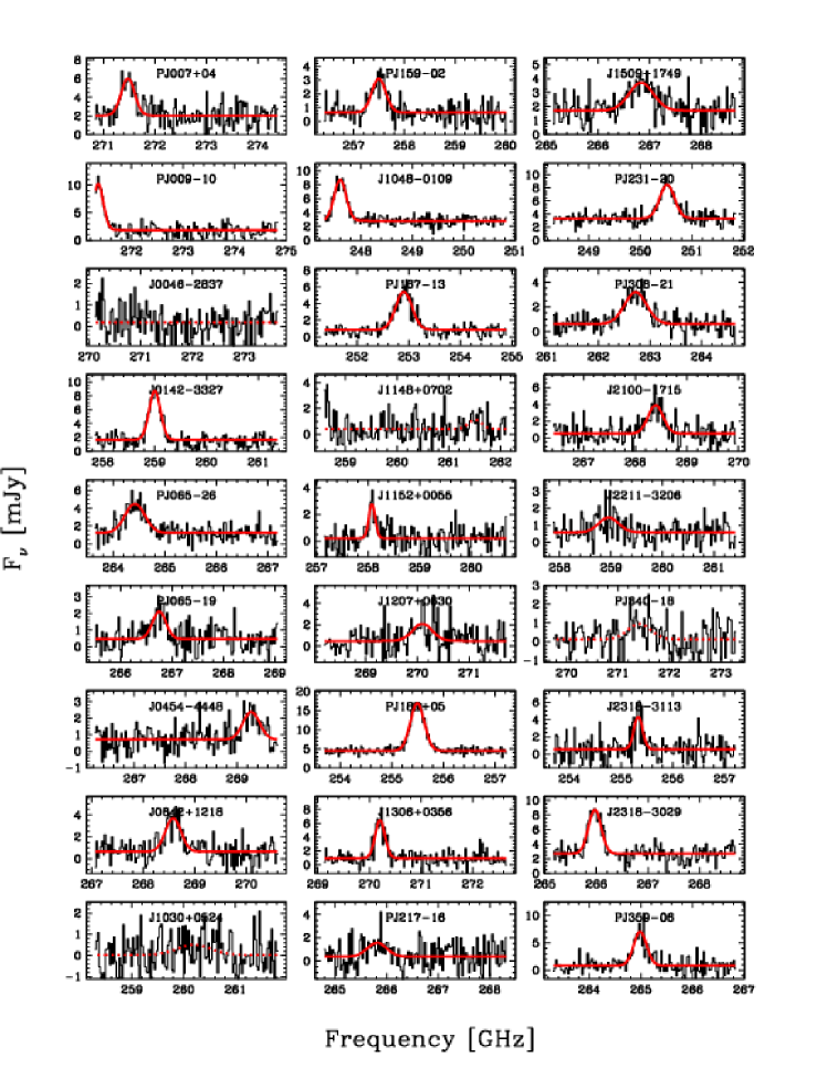
Figure 3: ALMA spectra of [C ii] and underlying continuum of the quasars in our sample (black histograms), plotted with a 30 km s^-1 velocity binning. The best fit Gaussian line+flat continuum models are shown as solid red lines. The fit values for continuum and line are summarized in Table 5. We also show with dotted lines the best fits in those cases where no significant line emission is detected.

3 Observations, data reduction and analysis

The ALMA data set (program ID: 2015.1.01115.S) used in this study consists of short ($\sim 8$ min on source) pointings centered on the optical/NIR coordinates of the quasars. The tuning frequency of the Spectral Windows (SPWs) was chosen as follows: Two SPWs (0 and 1) encompassed the expected observed frequency of [C ii], given our best pre–ALMA redshift estimate (see Table 2), with a small overlap (typically $<5$% of the bandwidth) between SPW 0 and 1 to account for noisy edge channels. This results in a frequency coverage of $\sim 3.6$ GHz around the expected observed frequency of the [C ii] line, or $\Delta z\approx 0.014$. At $z=6.5$, the [C ii] line ($\nu_{0}=1900.548$ GHz) is shifted to $\nu_{\rm obs}=253.406$ GHz. The other two SPWs (2 and 3) covered rest-frame frequencies around 1790 GHz. Observations were carried out between 2016 January and July, with the array in compact configuration with 38-49 12 m antennas. The primary beam of the 12m ALMA antennas is $\sim 25^{\prime\prime}$ in diameter at 250 GHz. The synthesized beam size is typically $\sim 1.1^{\prime\prime}\times 0.8^{\prime\prime}$. The typical rms noise is 0.5 mJy beam^-1 per 30 km s^-1 channel. Table 4 provides details on the observations, beam size, and sensitivity reached for each target.

We processed the data using the CASA (McMullin et al., 2007) pipeline for ALMA (version 4.7.1), using the default calibration procedure. The cubes were imaged using Briggs cleaning (via the CASA task tclean) with robustness parameter = 2 (i.e., natural visibility weights) to maximize the signal-to-noise ratio of our observations. The imaging process involves the following steps:

• First, we collapse SPWs 0 and 1 into a single continuum+line map for each target. This map is inspected in order to identify the position of detected sources, and to estimate the depth of the observations (via a 3-$\sigma$ clipped estimate of the map rms). A box mask is created around each detected source.

• We then image the data cube (coupling SPWs 0&1 and 2&3), using the mask to identify the cleaning regions, and adopting a 2-$\sigma$ cleaning threshold based on the continuum estimate (assuming roughly constant noise per channel throughout the cube). We adopt 30 km s^-1 channels with a linear interpolator in order to resample the cube in velocity space.

• We extract 1D spectra on a single-pixel basis centering at the position of the detected sources.

• We fit the extracted spectra with a flat continuum + a Gaussian.

• In order to create the line map, we collapse the data cube in the frequency range set by the line peak $\pm 1.4\,\sigma_{\rm line}$ from the best (spectral) fit. Here, $\sigma_{\rm line}$ is the line width from the Gaussian fit, giving a Full Width at Half Maximum FWHM$\approx$2.35 $\sigma_{\rm line}$. This choice maximizes the S/N of the line map, in the case of a perfectly Gaussian line profile, and constant noise. For a Gaussian line profile, integrating within $\pm 1.4\,\sigma_{\rm line}$ recovers 83% of the total line flux.

• We create a pure–continuum map by using the line–free channels in SPW 0&1, or the entire available bandwidth for SPWs 2&3. We opt not to combine all the continuum maps, in order to preserve information about the spectral slope.

• The pure–line map is obtained by subtracting (in uv-space) the continuum emission from the map created at step #5.

The continuum-subtracted line map of each target in our study is shown in Figure 2.

4 Results

For sources that are unresolved, or only marginally resolved, two different approaches can be used in order to infer a line flux. The first one is to extract the spectrum at a single spatial pixel (from step 3 of the imaging procedure described above), and fit the line profile along the frequency / velocity axis. The second approach consists of creating a line map, and fit the emission in the sky plane (as described in steps 5-7 of the imagine procedure). The first approach has the advantage that the full spectral information is taken into account (including potential wings in the line profile); on the other hand, it might suffer from flux losses if the emission is spatially extended. In contrast, the second approach captures the spatial extent of the line emission, but misses the wings along the spectral (i.e., velocity) dimension of the cubes. Here we adopt both approaches, and then estimate the impact of the underlying assumptions in order to establish the best estimate of the [C ii] line emission in the sources in our sample.

4.1 [C ii] spectral measurements

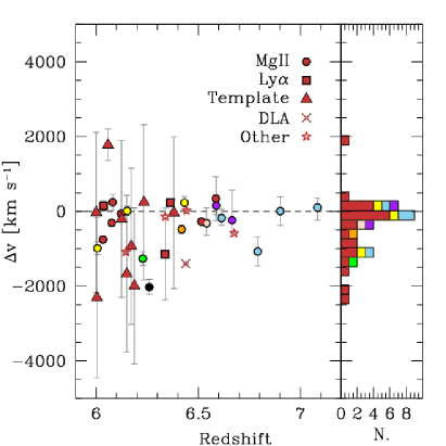
Figure 4: Velocity offset between the pre-ALMA redshift estimates of the quasars, and their [C ii]–based redshifts ($v_{\rm pre-ALMA}-v_{\rm[CII]}$). The different methods used in the pre-ALMA redshift estimates (mostly based on features associated with the broad–line region) are indicated by different symbols, while the color-coding highlights the reference for the [C ii] redshift using the same color–scheme of Figure 1. While part of the scatter is due to the large uncertainties in the pre-ALMA methods, we find significant shifts of several hundred km s^-1 in several quasars.

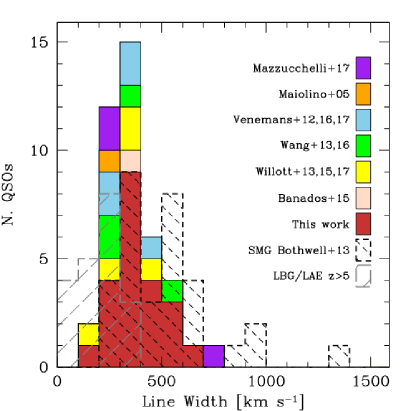
Figure 5: Distribution of the line width (FWHM) of [C ii] in the quasars of our sample, compared with the literature sample (indicated with different colors), and with the distribution of CO line widths in sub-mm galaxies from Bothwell et al. (2013) and of [C ii] line widths in $z>5$ Lyman Break Galaxies and Ly$\alpha$ Emitters (Riechers et al., 2014; Capak et al., 2015; Maiolino et al., 2015; Pentericci et al., 2016). The distributions of quasars and SMGs are statistically indistinguishable, whereas LBGs/LAEs show narrower lines.

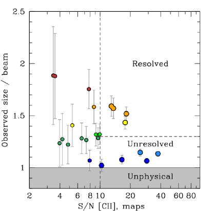
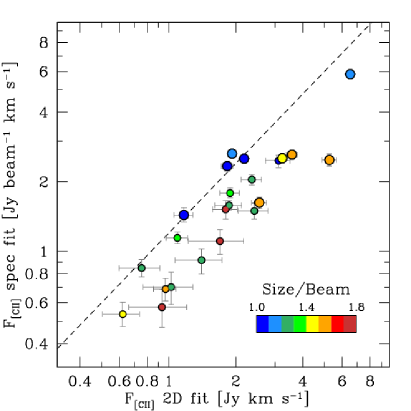
Figure 6: Size estimate of the [C ii]–emitting region and impact on single–pixel extractions. Left: The observed (i.e., beam-convolved) size estimated from the 2D Gaussian fit of the continuum–subtracted [C ii] line maps, plotted as a function of the signal–to–noise ratio of the line detection, as estimated from the maps. The color code of the points reflects the y-axis position of the points, while the bigger symbols highlight the objects with S/N$>$10. Right: The [C ii] flux measured from the single–pixel extraction of the spectra, and fitted with a Gaussian line profile (see Figure 3), as a function of the [C ii] flux measured with the 2D Gaussian fit of the line maps. The dashed line shows the one-to-one case, after applying a correction for the wings of the lines that have not been included in the maps. The symbol size and color scheme are the same as in the left–hand panel.

As described in the previous section, we first searched the collapsed continuum+line maps for sources, and extrated spectra at the position corresponding to the emission peak. This approach is justified as the size of the [C ii]–emitting regions in quasar host galaxies is comparable with the resolution element of our sources (Venemans et al., 2017a, see also Figure 6 in the present work). In those objects in which no clear detection associated with the quasar host galaxy was found, we extracted the spectra at the nominal position of the target based on optical/NIR data. The spectra, extracted over SPWs 0&1, of all the quasars in our study are shown in Figure 3.

We fit the spectra assuming a flat continuum emission from the dust, plus a Gaussian for the [C ii] line. We use a custom Metropolis Monte Carlo Markov Chain code to sample the posterior probability of the models, given the observed data. We adopt a flat prior for the line peak frequency, a Maxwellian distribution with a line width of 300 km s^-1, and a broad Gaussian distribution as prior for the flux density of both the line peak and the continuum. The fits and their uncertainties at 1-$\sigma$ significance are derived as the median and the 14%–86% quartiles of the posterior distribution. The resulting line parameters (peak frequency, width, flux) are reported in Table 5. We consider a line detected if its integrated flux exceeds 5 times its lower-side uncertainty. Out of 27 targeted quasars, 4 do not match this criterion: J0046-2837, J1030+0524, J1148+0702, and PJ340-18. The depths of these observations were not significantly different from the remainder of the sample.

Figure 4 shows the velocity difference between the pre–ALMA redshift estimates and their [C ii]–based redshifts. There is significant scatter, largely due to the rather large uncertainties of some pre–ALMA redshift estimates. This is particularly true for redshift estimates based on the Ly$\alpha$ features (in emission and/or absorption) only, or for quasars for which we only have optical spectroscopy (thus sampling only a few, generally fainter lines). A number of sources, however, show statistically–significant velocity differences of several hundred km s^-1 (and up to a few thousand km s^-1), with a tendency towards blue-shifts of the pre–ALMA estimators. This supports earlier evidence for such shifts (e.g., Riechers et al., 2011b; Venemans et al., 2016), but on a larger, homogeneous sample. The weighted average of the velocity offsets (including both our sample and the reference literature sources) is $-620\pm 8$ km s^-1 (accounting for the formal uncertainties in both the redshift estimates). Given that the pre–ALMA estimates are mostly based on features of the broad-line region, it is possible that these shifts are due to outflowing material or winds close to the central black holes.

The large differences observed between pre–ALMA and [C ii] redshifts may be responsible for at least part of the [C ii] non detections in our survey. The combination of SPWs 0&1 in the ALMA data results in a coverage of $\sim 4100$ km s^-1 at $z=6.0$. In fact, in the case of PJ009–10, J0454–4448, and J1048–0109, the [C ii] line is observed at the edge of the band, so it is possible that in some cases the line has just been missed by our observations. This is likely the case for J1148+0702, the redshift of which was revised after our observations were performed (Jiang et al., 2016). The other non–detections (J0046–2837, J1030+0524, and PJ340–18) also show the faintest dust continua in our survey, thus suggesting that they might be intrinsically faint in [C ii].

Figure 5 compares the distribution of [C ii] line widths (expressed as FWHM of the Gaussian fit) for the quasars in our sample, to the literature sample. The mean and standard deviations of the two distributions are $385\pm 115$ km s^-1 and $350\pm 125$ km s^-1, respectively. A Kolmogorov-Smirnov test suggests that the parent distribution from which the two samples are drawn is statistically indistiguishable. This is not surprising, as the majority of the sample of quasars from the literature fulfill both the redshift and the UV luminosity criteria used in the definition of our sample (see Section 2). Similarly, we compare the width distribution of [C ii] in $z>6$ quasars with the one of CO in sub-mm galaxies at $z=1-3$ from Bothwell et al. (2013). The latter shows a tail towards broader line widths compared with the former, but the difference is not statistically significant. On the other hand, Lyman Break Galaxies (LBGs) and Ly-$\alpha$ Emitters at $z>5$ (Riechers et al., 2014; Capak et al., 2015; Maiolino et al., 2015; Pentericci et al., 2016) show significantly narrow [C ii] lines, with a mean and standard deviation of $200\pm 100$ km s^-1.

4.2 [C ii] 2D measurements

We can also infer the line flux and the size of the [C ii]-emitting region via a fit of the continuum-subtracted maps shown in Figure 2. The fit is performed within CASA, selecting a narrow rectangular region around the quasars for the fit. Because the maps have been created by integrating over $2.8\times\sigma_{\rm line}$, for a gaussian line profile, only $\sim 83$% of the total line emission is enclosed in the maps – this factor is taken into account in our flux measurements. The intrinsic emission is modeled as a 2D-gaussian profile, with the centroid position, integrated flux, deconvolved major and minor axis, and the position angle as free parameters. The modeled emission is then convolved with the observed beam, when fitting to the data. The derived parameters are listed in Table 6.

The 2D Gaussian fits suggest that the sizes of the [C ii] emission are comparable to (and at most, twice as large as) the synthesized beams, suggesting that our [C ii] size estimates are only tentative. In Figure 6 we assess the impact of extended emission in our [C ii] flux estimates. First, we plot the ratio between the observed (i.e., beam–convolved) size and the beam major axis, as a function of the signal–to–noise ratio (S/N) of the [C ii] line as measured from the 2D fit. At S/N$>$10, we find 5 sources with compact [C ii] emission (observed size $\approx$ beam), and 4 with resolved emission on scales of $\sim 1.5\times$ the beam size. This difference in size is also reflected in the comparison between the [C ii] flux estimated from the single-pixel extraction of the spectrum, and the one based on the 2D Gaussian fit (see Figure 6, right): the more extended objects tend to deviate from the 1–to–1 relation. In the following, we define a source’s [C ii] flux through the measurement via the 2D spatial Gaussian fit, and scaling by a fixed $1/0.83\times$ factor to account for the flux associated with the wings of the line that are not included in the maps.

In Decarli et al. (2017), we presented the search for companion [C ii]–bright sources in the field of our observations. Out of 25 fields with comparable depth (i.e., excluding J2318-31 and J2318-30 because of inferior data quality), we found companion [C ii]–bright galaxies in 4 cases (J0842+1218, J2100–1715, PJ231–20, and PJ308–21). In two cases, the separation between the companion and the quasar host galaxy is $\sim 10$ kpc, or $\sim 2^{\prime\prime}$. Given the angular resolution of our data, it is possible that more companion galaxies are present at very small angular separation ($\sim 1^{\prime\prime}$) from other quasars (in particular, see the discussion on P167–13 in Willott et al., 2017). This would clearly affect our estimates of the size, surface brightness, and integrated luminosity of these sources.

5 Analysis

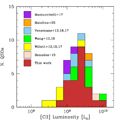
Figure 7: Distribution of [C ii] luminosity in our sample and in the sample from the literature. Typical line luminosities are in the range $(1-5)\times 10^{9}$ L_⊙. Only sources detected at $>$5-$\sigma$ (in the spectral fit, see Section 4.1) are shown.

5.1 [C ii] and continuum luminosities

The line fluxes are converted into line luminosities following:

$$\frac{L_{\rm[CII]}}{\rm L_{\odot}}=1.04\times 10^{-3}\,\frac{F_{\rm line}}{\rm Jy\,km\,s^{-1}}\,\frac{\nu_{\rm obs}}{\rm GHz}\,\left(\frac{D_{\rm L}}{\rm Mpc}\right)^{2},$$ (1)

where $F_{\rm line}$ is the integrated line flux (from the 2D fit of the line described in Section 4.2, corrected for the flux loss due to the line wings), $\nu_{\rm obs}$ is the observed frequency of the line, and $D_{\rm L}$ is the luminosity distance (see, e.g., Carilli & Walter, 2013). Figure 7 shows the distribution of [C ii] luminosity for the quasars in our main sample, and in the literature sample. The [C ii] lines of the quasars in our sample span over a dex in luminosity, with a peak in the distribution around $3\times 10^{9}$ L_⊙. This is consistent with the range of luminosities typically reported in similar sources from previous studies (see also Table 3), with the exception of the Willott et al. (2013, 2015) sample which focuses on sources fainter in the rest-frame UV and in the [C ii] emission than the ones selected here.

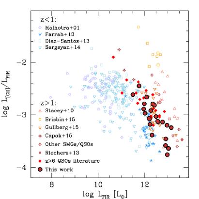
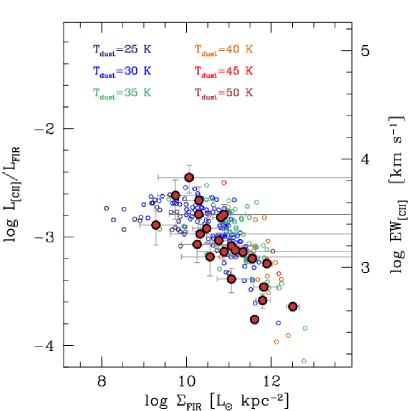
Figure 8: Left: The [C ii]–to–FIR luminosity ratio as a function of FIR luminosity, for the sources in our sample as well as a compilation of $z<1$ sources (blue/cyan symbols; data from: Malhotra et al. 2001, Farrah et al. 2013, Díaz-Santos et al. 2013, Sargsyan et al. 2014) as well as high-$z$ objects (red/orange symbols; data from: Stacey et al. 2010, Brisbin et al. 2015, Gullberg et al. 2015, Capak et al. 2015, Riechers et al. 2013, Riechers et al. 2014, Sargsyan et al. 2014). For all the samples, we do not plot upper limits for the sake of clarity. Quasars in our sample span a wide range (over a dex) of [C ii]/FIR ratio, ranging from ULIRG–like values ([C ii]/FIR$\sim$0.001) to values closer to local star-forming galaxies ([C ii]/FIR$\sim$0.01). This highlights the diversity in the global properties of the ISM in $z>6$ quasars. Right: The [C ii]/FIR ratio as a function of the FIR luminosity surface density, $\Sigma_{\rm FIR}$. Empty circles show the GOALS IR–luminous galaxies from Díaz-Santos et al. (2017), color–coded based on the dust temperature estimated from the $F_{\nu}$(63 $\mu$m)/$F_{\nu}$(158 $\mu$m) ratio.

By comparing the [C ii] emission with the underlying continuum, we gain important insights into the physical properties of the ISM in our sources. The most commonly used diagnostic in this context is the ratio between the [C ii] luminosity and the integrated luminosity of the underlying dust continuum. A detailed discussion of the dust continuum properties of the quasars in our sample is deferred to a companion paper (Venemans et al. in prep). Briefly, in order to infer IR luminosities, we model the dust continuum emission as a modified black body (see, e.g., Dunne et al., 2000; Beelen et al., 2006):

$$L_{\nu}({\rm dust})=\frac{2h\nu^{3}}{c^{2}}\,\kappa_{\nu}(\beta)\,\frac{M_{\rm dust}}{e^{h\nu/k_{\rm b}T_{\rm dust}}-1}$$ (2)

where $T_{\rm dust}=47$ K is the dust temperature, $\kappa_{\nu}(\beta)=0.77\,(\nu/{\rm 352\,GHz})^{\beta}$ cm² g^-1 is the opacity law, and $\beta=1.6$ is the (dust) emissivity index. The values of $T_{\rm dust}$ and $\beta$ assumed here are taken from Beelen et al. (2006), and are consistent with similar, more recent studies (e.g., Leipski et al., 2014). IR luminosities, $L_{\rm IR}$, are calculated by integrating equation 2 between 3 and 1100 $\mu$m (rest frame; see Kennicutt & Evans 2012). The far–IR luminosity $L_{\rm FIR}$ (integrated between 42.5 and 122.5 $\mu$m; see, e.g., Helou et al., 1988) is $L_{\rm FIR}=0.75\,L_{\rm IR}$ for our model. Given $T_{\rm dust}$ and $\beta$, we only need to normalize the continuum which we derive from the line–free channels at $\lambda_{0}\approx 158$ $\mu$m. This gives a dust mass as well (see Venemans et al. 2012, 2016 and in prep. for further discussion). In order to ensure a consistent analysis, we also re-compute FIR luminosities for all the other quasars in the literature sample, starting from the published measurements of the continuum flux density at 158 $\mu$m.

Another useful quantity in this context is the [C ii] (rest-frame) Equivalent Width (EW), defined as:

$$\frac{\rm EW}{\rm km\,s^{-1}}=1000\,\frac{F_{\rm line}\,{\rm[Jy\,km\,s^{-1}]}}{F_{\nu}({\rm cont})\,{\rm[mJy]}}.$$ (3)

The use of EWs has the practical advantage of circumventing any assumption of the shape of the dust SED. The inferred $L_{\rm[CII]}$, $L_{\rm FIR}$, and EW values for the targets in our sample are listed in Table 6.

Figure 8, left shows the [C ii]/FIR luminosity ratio as a function of the FIR luminosity. This is a widely used diagnostic of ISM properties. The [C ii]/FIR ratio is typically 0.003–0.01 in local, star-forming galaxies with modest dust temperature and luminosity, and drops by an order of magnitude towards the bright end (the so–called ‘[C ii] deficit’), in particular in the presence of high–temperature, compact dust emission (Malhotra et al., 2001; Farrah et al., 2013; Díaz-Santos et al., 2013, 2014, 2017; Sargsyan et al., 2014; Herrera-Camus et al., 2015). The quasars in our sample span a wide range (over 1 dex) of [C ii]/FIR values, from $\sim 0.0003$ as in local ULIRGs to $\sim 0.003$ as in local disk galaxies. This is consistent with what has been previously found for other smaller samples of $z>6$ quasars in the literature (e.g., Walter et al. 2009; Venemans et al. 2012, 2016; Wang et al. 2013, 2016; Willott et al. 2013, 2015; Bañados et al. 2015; Mazzucchelli et al. 2017).

In Section 5.7, we discuss the dependence of $L_{\rm[CII]}$ on the rest-frame UV luminosity of the quasars.

5.2 [C ii] and FIR luminosity surface density

An insight on the origin of the spread in the [C ii]/FIR values is offered by the relatively tight relation between the [C ii]/FIR and the FIR luminosity surface density, $\Sigma_{\rm FIR}$. We follow here the analysis presented by Díaz-Santos et al. (2017), who studied fine-structure lines and dust emission in a sample of $\sim 240$ IR–luminous galaxies at $z<0.1$ from the Great Observatories All-sky LIRG Survey (GOALS; Armus et al. 2009). We compute $\Sigma_{\rm FIR}=L_{\rm FIR}\,(2\pi R_{\rm cont}^{2})^{-1}$ based on the 2D Gaussian fit size of the continuum map (see Table 6). We emphasize that our observations only marginally resolve the emission in most of the sources. Díaz-Santos et al. (2017) show that the [C ii]/FIR ratio in galaxies from the GOALS sample correlates with dust temperature (parametrized based on the ratio between the dust flux densities at 63 $\mu$m and at 158 $\mu$m) and the compactness of the IR continuum emission. Galaxies with more compact IR continuum emission tend to show higher dust temperature and lower [C ii]/FIR ratio.

Our data generally follow the trend shown in Díaz-Santos et al. (2017) for local IR–luminous galaxies, with lower [C ii] equivalent widths associated with higher FIR surface densities. This might also reflect a diversity in the dust temperature in quasar host galaxies, with increasing dust temperature at decreasing [C ii]/FIR or [C ii] EW; however, the scatter is significant, and the present data do not support a straightforward derivation of $T_{\rm dust}$ from either $\Sigma_{\rm FIR}$ or the [C ii]/FIR ratio.

We can also infer the [C ii] luminosity surface density, $\Sigma_{\rm[CII]}$, using $R_{\rm[CII]}$, i.e., the half-size of the beam–deconvolved [C ii] emission. The resulting values are listed in Table 6.

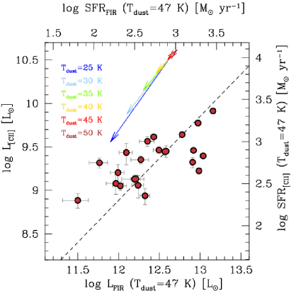
Figure 9: Comparison between the star-formation rate estimates derived from the [C ii] luminosity (following Herrera-Camus et al. 2015) and from the dust continuum luminosity (following Kennicutt & Evans 2012), in the assumption of $T_{\rm dust}=47$ K. The dashed line is the 1–to–1 case. The quasar host galaxies in our sample cover a range of about 1.5 dex in star formation rate. The two prescriptions for SFR estimates are correlated, although substantial scatter is present. The arrows show how the SFR estimates would change if we adopt different dust temperatures.

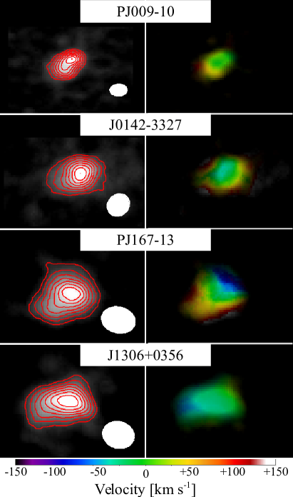
Figure 10: Moment zero (left) and one (right) maps of the four objects in our sample with S/N$>$10 in the 2D gaussian fit of the line, and with clearly resolved emission (observed size $>1.4\times$ the beam, see Figure 6). Here the maps have been re-imaged using robustness parameter = 0.5 to increase the angular resolution. In the moment zero maps, the contours mark the 30%, 40%, 50%, …90% of the peak emission. The beam of the observations is plotted in each panel for reference as a white ellipse. Each panel is $4.5^{\prime\prime}\times 3.5^{\prime\prime}$, corresponding to $\sim 25$ kpc $\times 20$ kpc at the redshift of these quasars. North is up, East to the left. The velocity maps have all the same color scale, centered at the bulk of the [C ii] emission. Clear velocity gradients are observed in PJ167-13 and J1306+0356, and to a minor extent also in PJ009-10 and J0142-3327.

5.3 Star formation rates

Both the [C ii] luminosity and the dust continuum luminosity have been used in the literature to infer the star-formation rates (SFRs) of galaxies. Observational advantages in using [C ii] are that 1) the line is bright and therefore easy to detect in a single frequency setting if the redshift of the source is known within a few thousand km s^-1, 2) it is ubiquitously found in galaxies, and 3) it is rarely affected by saturation or absorption, except in the densest starburst nuclei. However, the “deficit” of [C ii] emission in the brightest sources as well as its dependence on metallicity challenge its applicability as a SFR tracer (in particular for very luminous and compact starbursts, and for very metal–poor galaxies; see, e.g., De Looze et al. 2014; Herrera-Camus et al. 2015). Conversely, the photometric sampling of the dust continuum emission enables SFR estimates even in the absence of precise redshift information (see Kennicutt & Evans 2012 for a review on this topic). However, in order to effectively pin down the integrated dust emission, it is important to sample the dust SED close to its peak (rest-frame wavelengths $\lambda\mathrel{\hbox to0.0pt{\lower 3.0pt\hbox{$\sim$}\hss}\raise 2.0pt\hbox{$<$}}100$ $\mu$m), which is often challenging from the ground (as the frequencies of interest typically are $<500$ GHz, where the atmospheric transmission is limited).

Our [C ii]–based SFR estimates follow the fit to the [C ii]–SFR (24 $\mu$m–based) relation in 46 local galaxies from the KINGFISH sample (Kennicutt et al., 2011) derived by Herrera-Camus et al. (2015):

$$\frac{\rm SFR_{[CII]}}{\rm M_{\odot}\,yr^{-1}}=0.052\,\left(\frac{L_{\rm[CII]}\,\Psi(y)}{\rm 10^{40}\,erg\,s^{-1}}\right)^{1.034}$$ (4)

where $\Psi(y)=(y/y_{\rm t})^{\alpha}$ is a correction term dependent on dust temperature, with $y=\nu F_{\nu}$(70 $\mu$m)/$\nu F_{\nu}$(160 $\mu$m), $y_{\rm t}$=1.12, and $\alpha=1.2$. Adopting the calibration by De Looze et al. (2014) results in comparable SFR estimates.

For the dust–based SFR estimates, we follow Kennicutt & Evans (2012):

$$\frac{\rm SFR_{IR}}{\rm M_{\odot}\,yr^{-1}}=1.49\times 10^{-10}\,\frac{L_{\rm IR}}{\rm L_{\odot}}$$ (5)

In Figure 9, we compare the [C ii] and FIR luminosities and the corresponding SFRs, computed assuming $T_{\rm dust}=47$ K. The two estimates of SFR span approximately 1.5 dex and appear to correlate, although with substantial scatter. Different assumptions on the dust temperatures would affect both estimates of SFR in a similar way, leading to lower SFR values for lower dust temperatures.

The inferred SFR surface densities (the quantities in Figure 9 divided by our coarse estimates of the size of the emitting region) are always $<100$ M_⊙ yr^-1 kpc^-2, i.e., well below the theoretical Eddington limit ($\sim 1000$ M_⊙ yr^-1 kpc^-2; see, e.g., Scoville 2004, Thompson et al. 2005, Walter et al. 2009).

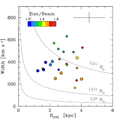
Figure 11: Line width (plotted as full width at half maximum) as a function of the radius of the [C ii]–emitting region ($R_{\rm[CII]}$) in the quasars in our sample. The color code is the same as in Figure 6. Sources with S/N$>$10 in the [C ii] map are highlighted with bigger symbols. Typical error bars are shown in the top–right corner. Under the assumption of rotation–dominated dynamics (see equation 7), the combination of these quantities yields an order-of-magnitude estimate of the dynamical mass enclosed within $R_{\rm[CII]}$, as shown by the loci of constant mass. We find dynamical masses of $2\times 10^{10}-2\times 10^{11}$ M_⊙. All but one of the high–S/N sources have $M_{\rm dyn}\approx 4\times 10^{10}$ M_⊙.

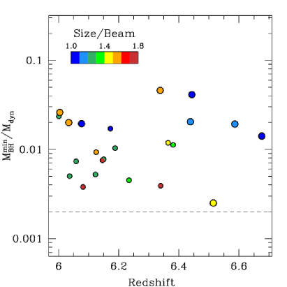
Figure 12: Constraints on the black hole – host galaxy mass ratio for the main sample of this work, as a function of the [C ii] redshift. The color code is the same as in Figs. 6 and 11. Objects with S/N$>$10 in the [C ii] map are highlighted with larger symbols. The minimum black hole mass $M_{\rm BH}^{min}$ is computed from the rest-frame UV continuum luminosity, by assuming that the quasars are emitting at Eddington luminosity. The dynamical mass is derived via equation 7, and might be considered as an upper limit for the marginally–resolved sources (blue points) or if the dynamics is dispersion supported (see equation 6). The plotted ratio can therefore be considered as a lower limit. The ratio observed in local galaxies is marked with a dashed line. All our quasars clearly lie above the local value. In particular, all but one of the high–S/N sources have $M_{\rm BH}^{\rm min}/M_{\rm dyn}\approx 0.03$, i.e., 1 dex above the local value.

5.4 Velocity maps and dynamical masses

Four sources in our sample are well–resolved in [C ii] (i.e., the observed size of the continuum–subtracted [C ii] emission from the 2D gaussian modeling is $>1.4\times$ the beam): PJ009–10, J0142–3327, PJ167–13, and J1306+0356 (see Figure 6). In Figure 10, we show the zero moment and the velocity field maps of these four sources. These are created after re-imaging the cubes using robustness parameter = 0.5, which increases the relative weights of the long baselines, thus improving the angular resolution of the imaged cubes. PJ009–10 shows an elongated morphology along the North-West – South-East axis. Its velocity map shows a small velocity gradient. Similarly, J0142–3327 appears extended along the East–West direction, but the velocity structure is less clear. On the other hand, PJ167–13 shows a clearly resolved velocity gradient from North-West towards South-East, with a peak–to–peak velocity difference exceeding 400 km s^-1 along the line of sight. J1306+0356 shows a velocity gradient along the East–West direction, although in this case the peak–to–peak velocity difference is lower ($\sim 200$ km s^-1). The resolution of the available data is insufficient to assess whether the kinematics of the [C ii]–emitting gas in the host galaxies of these two quasars are dominated by ordered rotation or if the underlying velocity structure is more complex (see, for instance, the high-resolution studies of $z>6$ quasars presented in Venemans et al. 2017a and Shao et al. 2017). In particular, given the present data quality it is impossible to rule out whether part of the spatially–resolved [C ii] emission is associated with a close satellite galaxy of the quasar host galaxy, similar to the cases discussed in Decarli et al. (2017).

We can make rough estimates of the host galaxy dynamical masses from our observations. The dynamical mass in a dispersion–dominated system can be expressed as:

$$M_{\rm dyn}=\frac{3}{2}\,\frac{R_{\rm[CII]}\sigma_{\rm line}^{2}}{G},$$ (6)

where $R_{\rm[CII]}$ is the radius of the [C ii]–emitting region (defined as the major semiaxis of the 2D Gaussian fit of the [C ii] map), $\sigma_{\rm line}$ is the line width from the gaussian fit of the [C ii] spectra, and $G$ is the gravitational constant. If the line width is dominated by rotation, the gas appears as a flat disk with an inclination angle $i$ (see, e.g., Wang et al., 2013; Willott et al., 2015). In this case:

$$M_{\rm dyn}=G^{-1}\,R_{\rm[CII]}\,(0.75\,{\rm FWHM}/\sin i)^{2}.$$ (7)

Here, 0.75 is a factor to scale the line FWHM to the width of the line at 20% of the peak, in the case of a Gaussian profile, following Willott et al. (2015). If we assume an inclination of $i=55^{\circ}$ (following Willott et al., 2015, who derived it as the median inclination angle from the Wang et al. (2013) sample), the dynamical mass inferred with equation 7 is $3.1\times$ larger than the one estimated with equation 6 (see de Blok & Walter 2014 for a detailed discussion on deriving dynamical mass constraints from unresolved observations).

In Figure 11 we show the [C ii] line width and size for the quasar host galaxies in our sample. These are comparable with the ones reported in the literature for $z>6$ quasar host galaxies (Walter et al., 2004; Wang et al., 2013; Willott et al., 2015; Venemans et al., 2017a). The combination of size and line width implies that the targeted host galaxies have dynamical masses in the range $2\times 10^{10}-2\times 10^{11}$ M_⊙, if we adopt equation 7. In particular, all but one of the sources detected with S/N$>$10 in the [C ii] map have $M_{\rm dyn}\approx 4\times 10^{10}$ M_⊙. We stress however that, given the limited angular resolution of our observations, the dynamical mass estimates in some of the sources in our sample might be overestimated.

5.5 Black hole to host galaxy mass ratio

In the local universe, the mass of black holes in galaxy nuclei correlates with the host galaxy stellar mass (as well as with other large-scale properties of the galaxy, such as the stellar velocity dispersion). The typical mass ratio is $M_{\rm BH}/M_{\rm host}\sim 0.002$ (e.g., Marconi & Hunt 2003; Häring & Rix 2004; Sani et al. 2011; Kormendy & Ho 2013; a factor $\sim 10$ lower according to Reines & Volonteri 2015). Whether this ratio evolves with redshift is a matter of debate. Observations of the host galaxy starlight in conditions of natural seeing (e.g., Decarli et al., 2010; Targett et al., 2012; Matsuoka et al., 2014), using adaptive optics (e.g., Falomo et al., 2005; Inskip et al., 2011), or capitalizing on the exquisite angular resolution of the Hubble Space Telescope (e.g., Dunlop et al., 2003; Bennert et al., 2011; Schramm & Silverman, 2013; Park et al., 2015), in some cases aided by natural magnification (Peng et al., 2006; Ding et al., 2017) point towards a higher black hole to host galaxy mass ratio in quasars at redshift $z=1$–$4$, compared to local relations (although some studies, e.g., Jahnke et al., 2009; Cirsternas et al., 2011, found no evidence for an evolution in the black hole to host galaxy mass ratio). Studies exploiting spatially–unresolved observations of the spectral energy distribution of fainter active galactic nuclei (e.g., Merloni et al., 2010) also suggest that black holes were ‘overmassive’ at high redshift compared with galaxies of the same stellar mass in the local universe. Spatially–resolved observations at mm and radio wavelengths of gas in the host galaxy of high–redshift quasars have enabled dynamical estimates of the host galaxies up to the highest redshifts (e.g., Walter et al., 2004; Schumacher et al., 2012; Wang et al., 2013; Willott et al., 2013, 2015; Venemans et al., 2016, 2017a; Shao et al., 2017). They all consistently find a tendency towards a higher $M_{\rm BH}/M_{\rm dyn}$ ratio in high redshift quasars than the value observed in local galaxies, with up to a factor $\sim 10$ discrepancy at $z>6$. This general consensus in the observations might however be undermined by selection biases: since high–redshift studies focus on luminous quasars, they might privilege galaxies hosting more massive black holes (which can reach higher luminosities, as their Eddington luminosity is also higher) than the average population. The works by Lauer et al. (2007), Decarli et al. (2010), Schulze & Wisotzki (2014), DeGraf et al. (2015), Shankar et al. (2016), and Volonteri & Reines (2016) extensively discuss these issues.

At $z>6$, black hole masses are usually inferred from spectroscopic observations of the Mgii broad emission line at 2796 Å, which is shifted in the NIR $K$ band (e.g. Willott et al., 2003; Shen, 2013; De Rosa et al., 2011, 2014; Mazzucchelli et al., 2017). The typical black hole mass is $\sim 10^{9}$ M_⊙, implying that these quasars radiate close to their Eddington limit (Jiang et al., 2007; De Rosa et al., 2011, 2014; Mazzucchelli et al., 2017). Sensitive NIR spectroscopy is not available for all the quasars in our sample yet (the results from our dedicated program will appear in Farina et al. in prep.). However, we can set tentative constraints on the black hole masses by requiring that their luminosity is lower than the Eddington luminosity. This allows us to infer a limit on the minimum black hole mass of the quasars in our sample:

$$\frac{M_{\rm BH}^{\rm min}}{\rm M_{\odot}}=\frac{L_{\rm bol}}{1.26\times 10^{38}\,{\rm erg\,s^{-1}}}.$$ (8)

We derive the bolometric luminosity from the observed flux density at 1450 Å, following the conversion derived by Runnoe et al. (2012) and recomputed in Venemans et al. (2016):

$$\log\frac{L_{\rm bol}}{\rm erg\,s^{-1}}=4.553+0.911\,\log\frac{\lambda L_{\lambda}(1450\,\AA)}{\rm erg\,s^{-1}}$$ (9)

We derive lower limits on the black hole masses of $M_{\rm BH}^{\rm min}$=$(0.3-3)\times 10^{9}$ M_⊙. In Figure 12 we compare these black hole mass limits with the host galaxy dynamical masses in the conservative case of rotationally–supported gas dynamics (equation 7). We find that the mass ratio between black holes and host galaxies is well above the value observed in the local universe. In particular, all but one of the sources detected at high S/N in [C ii] have a mass ratio of $>$0.03, i.e., $>$15 times higher than the value observed in the local universe ($>$120 times higher than the expected value using the local relations in Reines & Volonteri 2015). Using an isothermal model for the host galaxy dynamics instead (equation 6) would lead to even higher $M_{\rm BH}^{\rm min}/M_{\rm dyn}$ ratios.

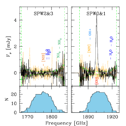
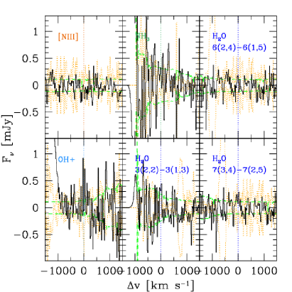
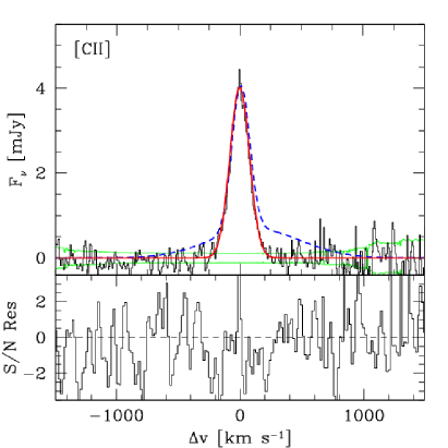
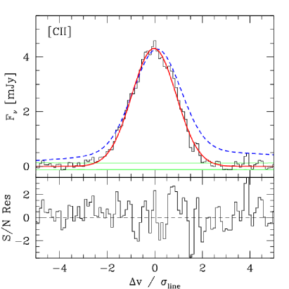
Figure 13: Stacked spectra at 1900 GHz of the [C ii]–detected quasars in our sample. We plot the stacked spectra as black histograms, their uncertainties (computed based on the noise of individual spectra) as green histograms, and the standard deviation (computed based on the variance between individual spectra) as orange, dotted histograms. Top left: Weighted–average stack of the individual spectra, shifted to rest frame based on the [C ii] redshift. Other lines that fall in the frequency range are marked. The bottom panels show the number of spectra used in the stack as a function of frequency. Top right: Zoom-in on the stacked spectrum of the quasar host galaxies in our sample, highlighting the expected frequencies of a number of other lines for which we have coverage. No detection is found for any of these lines. Bottom left: Weighted–average stack of individual [C ii] spectra, highlighting the [C ii] line. The best–fit Gaussian model of the stacked line is shown as a thick red line. For comparison, the [C ii] line profile of J1148+5251 as modeled in Cicone et al. (2015), showing a prominent outflow feature, is shown with a dashed blue line. The fit of J1148+5251 is normalized to match the peak flux density of the stacked [C ii] line in our sample. The bottom panel shows the residual from the fit, normalized by the noise per pixel. The stacked spectrum does not reveal any significant deviation from a Gaussian profile. Bottom right: Same as on the bottom–left panel, but this time stacking the spectra scaled by the width of each line. Also in this case, no significant deviation from Gaussianity is reported.

5.6 Stacked spectra

Figure 13 shows the stacked spectra of the quasars in our survey. We include only the [C ii]–detected sources as no other redshift indicator is precise enough for stacking (see Figure 4). After shifting all the observed spectra to the rest frame, we subtract the continuum (from the spectral fit), and average by weighting by the inverse of the variance (from the observed spectral noise). The uncertainty on the composite spectrum is obtained from the inverse square root of the sum of the weights. The resulting spectrum allows us to search for other faint lines in the rest-frame range 1775–1805 GHz (from SPW2&3) and 1890–1920 GHz (from SPW0&1). This range encompasses the fine structure lines of [Niii] 1789.806 GHz and [Niv] 1891.435 GHz; ammonia NH₃ lines at 1808.93 and 1810.38 GHz; the water lines H₂O 6(2,4)-6(1,5) at 1794.789 GHz, 7(3,4)-7(2,5) at 1797.159 GHz, 5(2,3)-4(3,2) at 1918.485 GHz, and 3(2,2)-3(1,3) at 1919.360 GHz; as well as a multiplet of OH+ lines at 1892.0–1892.2 GHz (blended with the [Niv] line). None of these transitions is significantly detected in our stacked spectrum. By integrating within $\pm 400$ km s^-1 around the nominal frequency of the lines, we obtain limits on the integrated flux of these lines in emission compared with the [C ii] line (see Table 1). We also do not detect these lines if we stack the continuum–normalized spectra (which allows us to search for the same lines in absorption). Similarly, by integrating the template based on continuum–normalized spectra within $\pm 400$ km s^-1 of the expected frequency of the lines, we infer limits on the equivalent widths of these lines (see Table 1). These limits are consistent with the few direct measurements and limits available for these transitions in galaxies in the literature. For example, in NGC 4418 and Arp 220 the H₂O 3(2,2)-3(1,3) line has EWs of $9.2\pm 2.3$ km s^-1 and $14.5\pm 0.9$ km s^-1, respectively (González-Alfonso et al., 2012). In HFLS-3 ($z=6.34$), all the water transitions discussed in our study are undetected, with limits on the EW of $<$1630 km s^-1 (Riechers et al., 2013).

Table 1: Limits on the strength of secondary lines covered in the stacked quasar spectra shown in Figure 13. (1) Transition ($X$). (2) Rest-frame frequency. (3) 5-$\sigma$ limit on the [C ii]/$X$ luminosity ratio. (4) 5-$\sigma$ limit on the equivalent width of transition $X$.

$X$	$\nu_{0}$	[C ii]/$X$	EW($X$)
	[GHz]		[km s-1]
(1)	(2)	(3)	(4)
[Niii]	1789.806	$>27$	$<44$
NH3	1808.93, 1810.38	$>9$	$<143$
OH+	1892.0-1892.2	$>19$	$<45$
H2O3(2,2)-3(1,3)	1919.360	$>10$	$<69$
H2O5(2,3)-4(3,2)	1918.485	$>10$	$<51$
H2O6(2,4)-6(1,5)	1794.789	$>25$	$<57$
H2O7(3,4)-7(2,5)	1797.159	$>25$	$<57$

We also create a second spectral template by scaling the velocity axis, so that all the [C ii] lines have the same width. We do so by scaling the abscissae of the individual spectra by the best-fit width of the [C ii] line $\sigma_{\rm line}$ (see Figure 13, bottom right).

The stacked spectra show no evidence of deviations from a Gaussian curve. We follow de Blok & Walter (2014) in order to put this result in the context of the geometry and kinematics of the [C ii]–emitting region. If the gas dynamics are supported by rotation in a disk, with the rotational velocity steeply increasing at small radii, and then flattening out at large radii (as seen in local spiral galaxies), we would naively expect a double–horned line profile, as observed in unresolved Hi observations of disk galaxies (e.g., Catinella et al., 2010). Its absence can be explained with the following arguments: 1) The gas is turbulent, i.e., the dispersion velocity term is at least comparable to the rotational velocity component along the line of sight; 2) The emission in the central beam of our observations captures a scale that is comparable with or smaller than the rising part of the velocity curve (i.e., $R_{\rm[CII]}\mathrel{\hbox to0.0pt{\lower 3.0pt\hbox{$\sim$}\hss}\raise 2.0pt\hbox{$<$}}h$, where $h$ is the scale length of the exponential disk, following the parametrization in de Blok & Walter 2014). These explanations are not mutually exclusive. High angular resolution observations of a few $z>6$ quasars revealed very compact [C ii] emission ($\sim 1$ kpc; see Walter et al., 2009; Venemans et al., 2017a; Shao et al., 2017), which favors the second scenario. Even when the [C ii] emission is clearly extended (e.g., J0305–3150, see Venemans et al. 2016; or P167–13 presented here), the luminosity–weighted size estimates available so far are in the $3-5$ kpc range, and extend only to a couple of beam radii. Observations with both higher angular resolutions and higher surface brightness sensitivity on large samples of quasars are needed in order to expose the faint, diffuse [C ii] emission on the outskirt of individual quasar host galaxies, thus allowing us to accurately constrain the global dynamical properties of these systems.

The lack of non-Gaussian components in the stacked [C ii] line profile has interesting implications in the search for outflows in the host galaxies of these quasars. J1148+5251 (Cicone et al., 2012, 2015) and Mrk231 (Feruglio et al., 2015) are remarkable examples of IR–bright quasars with non-Gaussian line profiles. In particular, Cicone et al. (2015) model the [C ii] line profile in J1148+5251 as the sum of narrow and broad components (see Figure 13). If such a feature were common in the quasars in our sample, we should clearly detect it in the stacked spectra. However, this is not the case, suggesting that J1148+5251 is unique compared to the bulk of the $z>6$ quasar population. No significant deviation from the Gaussian profile is detected in any of the individual spectra either (see Figure 3), with the caveat that some of the spectra only have a relatively modest S/N for this kind of analysis.

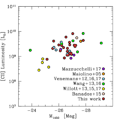
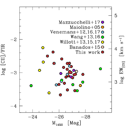
Figure 14: The dependence of the [C ii] luminosity and of the [C ii]/FIR ratio (or the [C ii] equivalent width) on the quasar UV luminosity, reported as absolute magnitude at 1450 Å in the rest frame. A weak correlation between UV and [C ii] luminosity is observed, although this is mostly driven by the inclusion of the Willott et al. (2013, 2015, 2017) sample at lower luminosities. The [C ii] equivalent width and [C ii]/FIR ratio show no correlation with the quasar UV luminosity.

5.7 [C ii] dependence on quasar UV luminosity

In Figure 14 we find a mild dependence of the [C ii] luminosity in our sample on the quasar UV luminosity, expressed in terms of the absolute magnitude at 1450 Å rest frame, $M_{1450}$. However, this conclusion is mostly driven by the contribution of the Willott et al. (2013, 2015) sample, that targets significantly lower UV and [C ii] luminosities. On the other hand, the [C ii] equivalent width (right panel) is practically independent of the quasar UV luminosity.

The lack of a correlation between the [C ii] equivalent width and the quasar UV luminosity may provide us with clues about the physical mechanisms responsible for heating the dust and for exciting the carbon ions. To first order, the more UV–luminous is the quasar, the higher are the dust temperature and the degree of carbon ionization (beyond the single ionization associated with the [C ii] line targeted here), thus we expect lower [C ii]/FIR luminosity ratio. From an empirical point of view, however, such a trend may break down if: 1) the observed UV emission of the quasar is (at least in some objects) affected by dust reddening along the line of sight; 2) the UV emission from the quasar boosts (instead of suppresses) the [C ii] emission in regions where the column densities are sufficient to shield photons with energy $E_{\gamma}>24.4$ eV (responsible for the second ionization of carbon); 3) the ISM in the host galaxy is multi-phase, in which a more extended and diffuse [C ii]–emitting region powered by star formation is superimposed on the central region which is strongly affected by the quasar radiation. This latter scenario is supported by the high [C ii]/[Ci]_2-1 ratios observed in some $z>6.5$ quasars, which are in tension with an X-ray–driven (i.e., AGN–powered) excitation of the gas (Venemans et al., 2017b).

6 Discussion & Conclusions

We presented a systematic study of the [C ii] line emission in 27 quasars at $z\mathrel{\hbox to0.0pt{\lower 3.0pt\hbox{$\sim$}\hss}\raise 2.0pt\hbox{$>$}}6$ with ALMA. This effort more than doubles the number of $z\mathrel{\hbox to0.0pt{\lower 3.0pt\hbox{$\sim$}\hss}\raise 2.0pt\hbox{$>$}}6$ quasars observed in [C ii] to date. Our main findings are:

• We detect [C ii] (and the dust underlying continuum) in 23 of the 27 targeted quasars (detection rate: $\sim 85$%) with [C ii] luminosities between $10^{9}$ and $10^{10}$ L_⊙. The typical [C ii] line width is $\sim 385$ km s^-1, similar to what has been found by previous studies.

• The [C ii]/FIR luminosity ratio (and the [C ii] equivalent width) range over $\sim 1$ dex, from very low ratios as in local ULIRGs up to higher ratios typical of normal star–forming galaxies. Despite the relatively low angular resolution of our observations, we find a dependence of the [C ii]/FIR ratio on the surface brightness of the IR emission, which mimics the results from low–redshift IR–luminous galaxies. In the low–$z$ comparison sample considered here, this ratio also depends on the dust temperature, which varies from $\sim$35 K to $\sim$50 K for [C ii]/FIR ratios comparable to those of the quasar host galaxies in our sample.

• We infer star formation rates and star formation surface densities $\Sigma_{\rm SFR}$ from both [C ii] and IR luminosities. None of our quasar host galaxies appears to have $\Sigma_{\rm SFR}$ approaching the Eddington limit, but the modest angular resolution of our data might be biasing our $\Sigma_{\rm SFR}$ low.

• Four sources are clearly spatially resolved, i.e., they have observed sizes of the [C ii]–emitting gas that are $\sim 1.4\times$ larger than the synthesized beam, and S/N$>$10. Two of them show clear velocity gradients. It is unclear whether these systems are dominated by rotation, or by a more complex dynamical pattern, or if the host galaxies have a [C ii]–emitting companion at a few kpc separation.

• A rough estimate of the dynamical mass of the host galaxies in our sample gives values between $2\times 10^{10}$ and $2\times 10^{11}$ M_⊙. By assuming Eddington–limited accretion, we estimate a minimum mass of the black holes powering the quasars in our sample, $M_{\rm BH}^{\rm min}=(0.3-3)\times 10^{9}$ M_⊙. The inferred mass ratio between the black holes and their host galaxies is thus $>15\times$ higher than that of local galaxies (e.g., Kormendy & Ho, 2013), consistent with previous findings based on CO (e.g., Walter et al., 2004).

• By stacking the spectra of all the [C ii]–detected quasar host galaxies in our sample, we put stringent limits on other lines (H₂O, OH+, [Niii], [Niv], NH₃). We do not detect any deviation from a Gaussian line profile for the [C ii] line. The strong outflow reported for an individual high–redshift quasar (J1148+5251, Cicone et al., 2015) thus does not appear to be a common feature of $z>6$ quasar hosts.

• The (rest-frame) UV luminosity of the quasar shows only a weak correlation with the [C ii] luminosity, and no correlation at all with the [C ii]/FIR ratio.

The 8 min on–source snapshot observations presented here demonstrate that bright dust and [C ii] emission are ubiquitous in quasar host galaxies at the highest redshifts currently accessible. Their brightness implies that early chemical enrichment in the hosts was a common phenomenon in the first Gyr of the Universe. Given their enormous flux densities, these sources are unique targets for future ALMA follow-up observations to obtain higher-resolution imaging of the ISM in the host galaxies, and to constrain the physical conditions in the ISM through multi-line observations.

Table 2: The main sample of this study. (1) quasar name. (2) Short name. (3-4) Right ascension and declination (J2000). (5) Optical/NIR redshift. (6) Method for optical/NIR redshift determination. (7) Redshift reference: 1- Bañados et al. (2016); 2- Venemans et al. (in prep); 3- Carnall et al. (2015); 4- Reed et al. (2017); 5- De Rosa et al. (2011); 6- Kurk et al. (2007); 7- Venemans et al. (2015); 8- Jiang et al. (2016); 9- Matsuoka et al. (2016); 10- Willott et al. (2010); 11- Mazzucchelli et al. (2017); 12- Kurk et al. (2009); 13- Becker et al. (2015); 14- Willott et al. (2009). (8) Absolute magnitude at rest-frame 1450 Å.

Name	Short name	RA	Dec	$z$	Method	Ref.	$M_{1450}$
		J2000.0	J2000.0				[mag]
(1)	(2)	(3)	(4)	(5)	(6)	(7)	(8)
PSO J007.0273+04.9571	P007+04	00:28:06.560	+04:57:25.68	$6.00\pm 0.05$	Template	1	-26.64
PSO J009.7355–10.4316	P009–10	00:38:56.522	-10:25:53.90	$5.95\pm 0.05$	Template	1	-26.53
VIK J0046–2837	J0046–2837	00:46:23.65	-28:37:47.34	$5.99\pm 0.05$	Template	2	-25.48
ATLAS J025.6821–33.4627	J0142–3327	01:42:43.73	-33:27:45.47	$6.31\pm 0.03$	Ly$\alpha$	3	-27.81
PSO J065.4085–26.9543	P065–26	04:21:38.052	-26:57:15.60	$6.14\pm 0.05$	Template	1	-27.25
PSO J065.5041–19.4579	P065–19	04:22:00.994	-19:27:28.68	$6.12\pm 0.05$	Template	1	-26.62
VDESJ0454–4448	J0454–4448	04:54:01.79	-44:48:31.1	$6.10\pm 0.01$	Template	4	-26.41
SDSS J0842+1218	J0842+1218	08:42:29.429	+12:18:50.50	$6.069\pm 0.002$	MgII	5	-26.91
SDSS J1030+0524	J1030+0524	10:30:27.098	+05:24:55.00	$6.308\pm 0.001$	MgII	6	-26.99
PSO J159.2257–02.5438	P159–02	10:36:54.191	-02:32:37.94	$6.38\pm 0.05$	Template	1	-26.80
VIK J1048–0109	J1048–0109	10:48:19.086	-01:09:40.29	$6.661\pm 0.005$	MgII	2	-26.00
PSO J167.6415–13.4960	P167–13	11:10:33.976	-13:29:45.60	$6.508\pm 0.001$	MgII	7	-25.62
ULAS J1148+0702	J1148+0702	11:48:03.286	+07:02:08.33	$6.339\pm 0.001$	MgII	8	-26.49
VIK J1152+0055	J1152+0055	11:52:21.269	+00:55:36.69	$6.37\pm 0.01$	Ly$\alpha$	9	-25.13
ULAS J1207+0630	J1207+0630	12:07:37.440	+06:30:10.37	$6.040\pm 0.003$	Ly$\alpha$	8	-26.63
PSO J183.1124+05.0926	P183+05	12:12:26.981	+05:05:33.49	$6.4039\pm 0.00001$	DLA	1	-27.03
SDSS J1306+0356	J1306+0356	13:06:08.258	+03:56:26.30	$6.016\pm 0.002$	MgII	6	-26.81
PSO J217.0891–16.0453	P217–16	14:28:21.394	-16:02:43.29	$6.11\pm 0.05$	Template	1	-26.93
CFHQS J1509–1749	J1509–1749	15:09:41.778	-17:49:26.80	$6.121\pm 0.002$	MgII	10	-27.14
PSO J231.6576–20.8335	P231–20	15:26:37.841	-20:50:00.66	$6.595\pm 0.015$	MgII	11	-27.20
PSO J308.0416–21.2339	P308–21	20:32:09.996	-21:14:02.31	$6.24\pm 0.05$	Template	1	-26.35
CFHQS J2100–1715	J2100–1715	21:00:54.616	-17:15:22.50	$6.087\pm 0.005$	MgII	10	-25.55
VIK J2211–3206	J2211–3206	22:11:12.391	-32:06:12.94	$6.336\pm 0.005$	MgII	2	-26.71
PSO J340.2041–18.6621	P340–18	22:40:48.997	-18:39:43.81	$6.01\pm 0.05$	Template	1	-26.42
VIK J2318–3113	J2318–3113	23:18:18.351	-31:13:46.35	$6.444\pm 0.005$	MgII	2	-26.11
VIK J2318–3029	J2318–3029	23:18:33.100	-30:29:33.37	$6.12\pm 0.05$	Template	2	-26.21
PSO J359.1352–06.3831	P359–06	23:56:32.455	-06:22:59.26	$6.15\pm 0.05$	Template	1	-26.79

Table 3: The sample from the literature. (1) quasar name. (2-3) Right ascension and declination (J2000). (4) Redshift. (5) Absolute magnitude at 1450 Å rest-frame. (6) [C ii] luminosity. (7) [C ii] Full Width at Half Maximum. (8) Total IR luminosity. (9) Reference: 1- Mazzucchelli et al. (2017); 2- Willott et al. (2015); 3- Wang et al. (2016); 4- Venemans et al. (2016); 5- Wang et al. (2013); 6- Willott et al. (2013); 7- Bañados et al. (2015); 8- Venemans et al. (2012); 9- Walter et al. (2009); 10- Willott et al. (2017); 11- Venemans et al. (2017c).

Name	RA	Dec	$z$	$M_{1450}$	$L_{\rm[CII]}$	FWHM([C ii])	log $L_{\rm TIR}$	Ref
	J2000.0	J2000.0		[mag]	[$\times 10^{9}$ L⊙]	[km s-1]	[L⊙]
(1)	(2)	(3)	(4)	(5)	(6)	(7)	(8)	(9)
P006+39	00:24:29.772	+39:13:18.98	6.6100	-26.9	$0.9\pm 0.5$	$280\pm 140$	$12.05\pm 0.17$	1
J0055+0146	00:55:02.910	+01:46:18.30	6.0060	-24.81	$0.827\pm 0.13$	$359\pm 45$	$11.58\pm 0.08$	2
J0100+2802	01:00:13.027	+28:02:25.84	6.3258	-29.14	$3.56\pm 0.49$	$300\pm 77$	$12.42\pm 0.09$	3
J0109–3047	01:09:53.131	–30:47:26.32	6.7909	-25.64	$2.4\pm 0.2$	$340\pm 36$	$12.08\pm 0.09$	4
J0129–0035	01:29:58.510	–00:35:39.70	5.7787	-23.89	$1.9\pm 0.3$	$194\pm 12$	$12.64\pm 0.010$	5
J0210–0456	02:10:13.190	–04:56:20.90	6.4323	-24.53	$0.29\pm 0.041$	$189\pm 18$	$11.38\pm 0.15$	6
P036+03	02:26:01.876	+03:02:59.39	6.5412	-27.33	$5.8\pm 0.7$	$360\pm 50$	$12.71\pm 0.11$	7
J0305–3150	03:05:16.916	–31:50:55.90	6.6145	-26.18	$3.9\pm 0.2$	$255\pm 12$	$12.83\pm 0.013$	4
J1044–0125	10:44:33.042	–01:25:02.20	5.7847	-27.38	$1.6\pm 0.4$	$420\pm 80$	$12.72\pm 0.013$	5
J1120+0641	11:20:01.479	+06:41:24.30	7.0842	-26.63	$1.3\pm 0.2$	$235\pm 35$	$12.15\pm 0.13$	8
J1148+5251	11:48:16.652	+52:51:50.44	6.4189	-27.62	$4.2\pm 0.35$	$287\pm 28$	$13.00\pm 0.06$	9
J1319+0950	13:19:11.302	+09:50:51.49	6.1330	-27.05	$4.4\pm 0.9$	$515\pm 81$	$12.99\pm 0.008$	5
J1342+0928	13:42:08.100	+09:28:38.61	7.5413	-26.76	$1.6\pm 0.2$	$383\pm 56$	$12.10\pm 0.20$	11
J2054–0005	20:54:06.481	–00:05:14.80	6.0391	-26.21	$3.3\pm 0.5$	$243\pm 10$	$12.73\pm 0.007$	5
P323+12	21:32:33.191	+12:17:55.26	6.5850	-27.12	$1.2\pm 0.3$	$250\pm 30$	$11.99\pm 0.16$	1
VIMOS2911	22:19:17.227	+01:02:48.88	6.1492	-23.10	$2.59\pm 0.13$	$264\pm 15$	$12.24\pm 0.03$	10
J2229+1457	22:29:01.649	+14:57:08.99	6.1517	-24.78	$0.594\pm 0.077$	$351\pm 39$	$11.00\pm 0.33$	2
P338+29	22:32:55.150	+29:30:32.23	6.6580	-26.14	$2.0\pm 0.1$	$740\pm 310$	$12.31\pm 0.11$	1
J2310+1855	23:10:38.882	+18:55:19.70	6.0031	-27.8	$8.7\pm 1.4$	$393\pm 21$	$13.20\pm 0.004$	5
J2329–0301	23:29:08.275	–03:01:58.80	6.4170	-25.25	$0.39\pm 0.04$	$477\pm 64$	$10.95_{-0.30}^{+0.17}$	10
J2348–3054	23:48:33.334	–30:54:10.24	6.9018	-25.8	$1.9\pm 0.3$	$405\pm 69$	$12.63\pm 0.03$	4

Table 4: Observing log, integration time, beam (major $\times$ minor axis, Position Angle), and noise rms (computed as the median of the rms values measured in the SPW0&1 channels, with 30 km s^-1 binning).

Short name	Date Obs.	Exp.Time	Beam	Beam PA	rms (30 km s-1)
		[min]	[′′]	[deg]	[mJy beam-1]
(1)	(2)	(3)	(4)	(5)	(6)
PJ007+04	19 Jun 2016	7.56	$0.66\times 0.46$	66.0	0.64
PJ009–10	19 Jun 2016	8.57	$0.63\times 0.43$	84.2	0.59
J0046–2837	07 Jul 2016	8.57	$0.49\times 0.41$	-86.9	0.49
J0142–3327	14 Apr 2016	8.06	$0.84\times 0.73$	-49.4	0.54
PJ065–26	29 Jan 2016	8.06	$1.10\times 0.83$	89.1	0.59
	31 Mar 2016	8.06
PJ065–19	01 Feb 2016	8.06	$1.07\times 0.71$	-78.4	0.47
	09 Apr 2016	8.06
J0454–4448	29 Jan 2016	8.57	$1.13\times 0.77$	89.0	0.47
	22 Mar 2016	8.57
J0842+1218	31 Jan 2016	7.56	$1.20\times 1.06$	77.5	0.65
J1030+0524	29 Jan 2016	8.57	$1.16\times 0.94$	64.0	0.58
PJ159–02	29 Jan 2016	8.57	$1.23\times 0.94$	67.6	0.44
J1048–0109	29 Jan 2016	12.10	$1.40\times 0.97$	64.0	0.42
PJ167–13	29 Jan 2016	8.06	$1.23\times 0.93$	76.1	0.42
J1148+0702	30 Jan 2016	8.57	$1.25\times 1.11$	87.0	0.55
J1152+0055	30 Jan 2016	8.06	$1.23\times 0.99$	-85.4	0.56
J1207+0630	31 Jan 2016	7.56	$1.54\times 0.83$	57.8	0.65
PJ183+05	27 Jan 2016	8.57	$1.19\times 1.00$	-89.7	0.50
J1306+0356	27 Jan 2016	8.57	$1.11\times 0.91$	74.4	0.56
PJ217–16	27 Jan 2016	8.57	$1.15\times 0.88$	78.4	0.64
J1509–1749	31 Jan 2016	8.06	$1.35\times 0.87$	65.0	0.50
PJ231–20	27 Jan 2016	7.56	$1.24\times 0.89$	74.9	0.58
PJ308–21	27 Mar 2016	12.60	$0.85\times 0.65$	79.2	0.46
J2100–1715	26 Mar 2016	8.06	$0.74\times 0.63$	-86.5	0.72
J2211–3206	30 Mar 2016	8.06	$0.87\times 0.70$	83.1	0.44
PJ340–18	09 Apr 2016	8.06	$0.78\times 0.66$	84.4	0.59
J2318–3113	02 Apr 2016	8.06	$0.83\times 0.77$	-87.2	1.04
J2318–3029	12 Apr 2016	8.06	$0.86\times 0.74$	-53.1	0.84
PJ359–06	27 Apr 2016	8.06	$1.08\times 0.61$	67.4	0.86

Table 5: Results from the spectral fit. These measurements are not corrected for extended emission. (1) Quasar name. (2) Line peak frequency. (3) Inferred [C ii] redshift. (4) Line Full Width at Half Maximum. (5) Integrated line flux. (6) Continuum flux density at 158$\mu$m (rest frame).

Short Name	$\nu_{\rm obs}$([C ii])	$z_{\rm[CII]}$	FWHM([C ii])	$F_{\rm line}$([C ii])	$F_{\nu}$(cont)
	[GHz]		[km s-1]	[Jy km s-1]	[mJy]
(1)	(2)	(3)	(4)	(5)	(6)
P007+04	$271.478_{-0.016}^{+0.015}$	$6.0008_{-0.0004}^{+0.0004}$	$340_{-36}^{+36}$	$1.58_{-0.07}^{+0.08}$	$2.07_{-0.04}^{+0.04}$
P009-10	$271.356_{-0.016}^{+0.015}$	$6.0039_{-0.0004}^{+0.0004}$	$251_{-34}^{+34}$	$2.49_{-0.15}^{+0.15}$	$1.89_{-0.07}^{+0.03}$
J0046–2837	—	—	—	—	$0.18_{-0.04}^{+0.04}$
J0142–3327	$259.004_{-0.015}^{+0.014}$	$6.3379_{-0.0004}^{+0.0004}$	$300_{-31}^{+32}$	$2.62_{-0.06}^{+0.06}$	$1.65_{-0.04}^{+0.04}$
P065–26	$264.417_{-0.018}^{+0.018}$	$6.1877_{-0.0005}^{+0.0005}$	$517_{-43}^{+44}$	$2.05_{-0.11}^{+0.10}$	$1.23_{-0.05}^{+0.05}$
P065–19	$266.753_{-0.023}^{+0.021}$	$6.1247_{-0.0006}^{+0.0006}$	$345_{-61}^{+67}$	$0.69_{-0.08}^{+0.08}$	$0.46_{-0.04}^{+0.05}$
J0454–4448	$269.272_{-0.022}^{+0.022}$	$6.0581_{-0.0006}^{+0.0006}$	$426_{-55}^{+57}$	$0.85_{-0.07}^{+0.08}$	$0.71_{-0.05}^{+0.05}$
J0842+1218	$268.580_{-0.019}^{+0.019}$	$6.0763_{-0.0005}^{+0.0005}$	$396_{-44}^{+45}$	$1.44_{-0.10}^{+0.11}$	$0.65_{-0.05}^{+0.06}$
J1030+0524	—	—	—	—	$0.03_{-0.05}^{+0.06}$
P159–02	$257.496_{-0.017}^{+0.017}$	$6.3809_{-0.0005}^{+0.0005}$	$373_{-39}^{+40}$	$1.15_{-0.07}^{+0.07}$	$0.65_{-0.03}^{+0.03}$
J1048–0109	$247.598_{-0.015}^{+0.014}$	$6.6759_{-0.0004}^{+0.0005}$	$330_{-33}^{+32}$	$2.52_{-0.06}^{+0.07}$	$2.84_{-0.04}^{+0.03}$
P167–13	$252.907_{-0.016}^{+0.014}$	$6.5148_{-0.0004}^{+0.0005}$	$437_{-34}^{+34}$	$2.53_{-0.07}^{+0.07}$	$0.87_{-0.05}^{+0.02}$
J1148+0702	—	—	—	—	$0.41_{-0.05}^{+0.05}$
J1152+0055	$258.076_{-0.017}^{+0.016}$	$6.3643_{-0.0004}^{+0.0005}$	$167_{-44}^{+45}$	$0.54_{-0.06}^{+0.07}$	$0.22_{-0.05}^{+0.04}$
J1207+0630	$270.094_{-0.032}^{+0.034}$	$6.0366_{-0.0009}^{+0.0008}$	$489_{-72}^{+78}$	$0.92_{-0.12}^{+0.11}$	$0.50_{-0.06}^{+0.06}$
P183+05	$255.497_{-0.015}^{+0.013}$	$6.4386_{-0.0004}^{+0.0004}$	$374_{-30}^{+30}$	$5.84_{-0.08}^{+0.08}$	$4.47_{-0.02}^{+0.02}$
J1306+0356	$270.207_{-0.015}^{+0.014}$	$6.0337_{-0.0004}^{+0.0004}$	$246_{-31}^{+31}$	$1.63_{-0.09}^{+0.09}$	$0.94_{-0.05}^{+0.07}$
P217–16	$265.817_{-0.040}^{+0.038}$	$6.1498_{-0.0010}^{+0.0011}$	$491_{-75}^{+74}$	$0.70_{-0.11}^{+0.11}$	$0.37_{-0.06}^{+0.06}$
J1509–1749	$266.838_{-0.024}^{+0.024}$	$6.1225_{-0.0006}^{+0.0007}$	$631_{-68}^{+72}$	$1.50_{-0.12}^{+0.11}$	$1.72_{-0.05}^{+0.05}$
P231–20	$250.520_{-0.016}^{+0.015}$	$6.5864_{-0.0005}^{+0.0005}$	$404_{-37}^{+39}$	$2.65_{-0.12}^{+0.11}$	$3.36_{-0.04}^{+0.05}$
P308–21	$262.720_{-0.019}^{+0.018}$	$6.2341_{-0.0005}^{+0.0005}$	$570_{-43}^{+45}$	$1.79_{-0.08}^{+0.10}$	$0.64_{-0.05}^{+0.03}$
J2100–1715	$268.393_{-0.020}^{+0.018}$	$6.0812_{-0.0005}^{+0.0005}$	$382_{-47}^{+51}$	$1.52_{-0.14}^{+0.14}$	$0.52_{-0.06}^{+0.06}$
J2211–3206	$258.952_{-0.037}^{+0.036}$	$6.3394_{-0.0010}^{+0.0010}$	$529_{-100}^{+118}$	$0.57_{-0.11}^{+0.11}$	$0.57_{-0.04}^{+0.05}$
P340–18	—	—	—	—	$0.13_{-0.05}^{+0.05}$
J2318–3113	$255.330_{-0.019}^{+0.018}$	$6.4435_{-0.0005}^{+0.0005}$	$234_{-49}^{+49}$	$1.11_{-0.14}^{+0.13}$	$0.57_{-0.08}^{+0.09}$
J2318–3029	$265.968_{-0.016}^{+0.015}$	$6.1458_{-0.0004}^{+0.0004}$	$320_{-34}^{+33}$	$2.34_{-0.11}^{+0.12}$	$2.71_{-0.08}^{+0.07}$
P359–06	$264.988_{-0.017}^{+0.015}$	$6.1722_{-0.0004}^{+0.0004}$	$330_{-37}^{+39}$	$2.47_{-0.16}^{+0.13}$	$0.87_{-0.07}^{+0.09}$

Table 6: Results from the 2D gaussian fit of the [C ii] continuum–subtracted line maps. (1) quasar name. (2) S/N of the line detection. (3) Observed (= beam-convolved) size of the [C ii]–emitting region from 2D gaussian fit of the continuum–subtracted line maps. (4) Beam-deconvolved size of the [C ii]–emitting region. (5) Radius of the [C ii] emission. (6) Measured [C ii] flux from the 2D gaussian fit. (7) [C ii] flux from the 2D gaussian fit, corrected to account for the flux loss due to the line wings not covered in the line maps. (8) [C ii] luminosity. (9) FIR luminosity. (10) FIR surface luminosity. (11) [C ii] Equivalent Width, in km s^-1.

Short name	S/N	[C ii] size	[C ii] dec. size	$R_{\rm[CII]}$	$F_{\rm[CII]}$(2D)	$F_{\rm[CII]}$(corr)	log $L_{\rm[CII]}$	log $L_{\rm FIR}$	log $\Sigma_{\rm FIR}$	log EW[CII]
	([C ii])	[′′]	[′′]	[kpc]	[Jy km s-1]	[Jy km s-1]	[L⊙]	[L⊙]	[L⊙ kpc-2]	[km s-1]
(1)	(2)	(3)	(4)	(5)	(6)	(7)	(8)	(9)	(10)	(11)
PJ007+04	21	$0.84\times 0.60$	$0.54\times 0.34$	1.6	$1.87\pm 0.26$	$2.24\pm 0.31$	9.25	12.91	11.80	$2.76_{0.07}^{0.06}$
PJ009–10	17	$0.99\times 0.72$	$0.82\times 0.47$	2.4	$5.26\pm 0.39$	$6.31\pm 0.47$	9.70	12.97	11.55	$3.15_{0.05}^{0.04}$
J0046–2837	—	—	—	—	—	—	—	11.46	—	—
J0142–3327	41	$1.28\times 0.90$	$0.98\times 0.48$	2.7	$3.57\pm 0.20$	$4.29\pm 0.24$	9.56	12.78	11.33	$3.23_{0.04}^{0.04}$
PJ065–26	18	$1.41\times 1.02$	$0.90\times 0.56$	2.5	$2.36\pm 0.25$	$2.83\pm 0.30$	9.37	12.57	11.15	$3.24_{0.06}^{0.05}$
PJ065–19	9	$1.69\times 0.76$	$1.32\times 0.26$	3.7	$0.97\pm 0.11$	$1.16\pm 0.13$	8.97	12.02	10.32	$3.38_{0.11}^{0.09}$
J0454–4448	12	$1.38\times 1.04$	$0.92\times 0.50$	2.6	$0.76\pm 0.16$	$0.91\pm 0.19$	8.86	12.33	11.06	$2.96_{0.12}^{0.10}$
J0842+1218	15	$1.23\times 1.21$	$0.61\times 0.15$	1.7	$1.17\pm 0.11$	$1.41\pm 0.14$	9.05	12.20	10.25	$3.28_{0.17}^{0.12}$
J1030+05	4	—	—	—	—	—	—	11.53	—	—
PJ159–02	17	$1.62\times 1.20$	$1.12\times 0.64$	3.1	$1.09\pm 0.12$	$1.31\pm 0.14$	9.05	12.21	11.06	$3.29_{0.08}^{0.07}$
J1048–0109	43	$1.49\times 1.13$	$0.60\times 0.49$	1.6	$2.18\pm 0.08$	$2.62\pm 0.09$	9.38	12.92	11.82	$2.93_{0.02}^{0.02}$
PJ167–13	35	$1.76\times 1.32$	$1.37\times 0.78$	3.7	$3.23\pm 0.18$	$3.88\pm 0.22$	9.54	12.43	10.81	$3.56_{0.05}^{0.04}$
J1148+0702	3	—	—	—	—	—	—	12.19	—	—
J1152+0055	9	$1.73\times 1.46$	$1.30\times 0.98$	3.6	$0.62\pm 0.12$	$0.75\pm 0.14$	8.81	11.50	9.74	$3.78_{0.22}^{0.14}$
J1207+0630	8	$1.96\times 1.24$	$1.23\times 0.90$	3.5	$1.40\pm 0.33$	$1.68\pm 0.40$	9.13	11.99	10.29	$3.56_{0.16}^{0.12}$
PJ183+05	70	$1.35\times 1.21$	$0.74\times 0.57$	2.0	$6.52\pm 0.17$	$7.83\pm 0.21$	9.83	13.16	11.90	$3.13_{0.017}^{0.016}$
J1306+0356	17	$1.77\times 1.21$	$1.41\times 0.73$	4.0	$2.55\pm 0.20$	$3.06\pm 0.24$	9.38	12.50	10.76	$3.32_{0.08}^{0.07}$
PJ217–16	6	$1.42\times 1.07$	$1.02\times 0.16$	2.9	$1.03\pm 0.26$	$1.23\pm 0.31$	9.00	11.97	9.28	$3.47_{0.18}^{0.13}$
J1509–1749	13	$1.73\times 1.34$	$1.09\times 1.01$	3.1	$2.42\pm 0.37$	$2.91\pm 0.44$	9.37	12.59	10.89	$3.22_{0.08}^{0.07}$
PJ231–20	23	$1.42\times 1.04$	$0.80\times 0.37$	2.2	$1.92\pm 0.08$	$2.31\pm 0.09$	9.32	13.04	12.51	$2.74_{0.04}^{0.04}$
PJ308–21	23	$1.12\times 1.01$	$0.81\times 0.69$	2.3	$1.89\pm 0.19$	$2.26\pm 0.23$	9.27	12.27	10.48	$3.44_{0.13}^{0.10}$
J2100–1715	11	$1.30\times 0.81$	$1.08\times 0.48$	3.1	$1.80\pm 0.23$	$2.16\pm 0.28$	9.24	11.77	10.06	$3.90_{0.15}^{0.11}$
J2211–3206	5	$1.64\times 1.15$	$1.47\times 0.78$	4.1	$0.93\pm 0.27$	$1.12\pm 0.33$	8.98	12.24	10.56	$3.18_{0.18}^{0.13}$
PJ340–18	4	—	—	—	—	—	—	11.60	—	—
J2318–3113	8	$1.56\times 1.45$	$1.35\times 1.20$	3.7	$1.70\pm 0.47$	$2.04\pm 0.57$	9.25	12.46	11.61	$2.61_{0.04}^{0.03}$
J2318–3029	21	$0.93\times 0.81$	$0.44\times 0.23$	1.2	$1.83\pm 0.11$	$2.20\pm 0.13$	9.25	12.92	10.29	$3.69_{0.18}^{0.13}$
PJ359–06	15	$1.15\times 1.06$	$0.91\times 0.29$	2.6	$3.11\pm 0.39$	$3.73\pm 0.47$	9.49	12.36	10.89	$3.56_{0.12}^{0.09}$

References

- Armus et al. (2009) Armus L., Mazzarella J.M., Evans A.S., et al. 2009, PASP, 121, 559
- Bañados et al. (2015) Bañados E., Decarli R., Walter F., Venemans B.P., Farina E.P., Fan X. 2015, ApJ, 805, L8
- Bañados et al. (2016) Bañados E., Venemans B.P., Decarli R., Farina E.P., Mazzucchelli C., Walter F., Fan X., Stern D., Schlafly E., Chambers K.C., et al. 2016, ApJS, 227, 11
- Bañados et al. (2017) Bañados E., Venemans B.P., Mazzucchelli C., Farina E.P., Walter F., Wang F., Decarli R., et al. 2017, Nature, in press
- Barnett et al. (2015) Barnett R., Warren S.J., Banerji M., McMahon R.G., Hewett P.,C. Mortlock D.J., Simpson C., Venemans B.P., et al. 2015, A&A, 575, A31
- Barvainis et al. (1997) Barvainis R., Maloney P., Antonucci R., Alloin D., 1997, ApJ, 484, 695
- Becker et al. (2015) Becker G.D., Bolton J.S., Madau P., Pettini M., Ryan-Weber E.V., Venemans B.P. 2015, MNRAS, 447, 3402
- Beelen et al. (2006) Beelen A., Cox P., Benford D.J., Dowell C.D., Kovács A., Bertoldi F., Omont A., Carilli C.L. 2006, ApJ, 642, 694
- Bennert et al. (2011) Bennert V.N., Auger M.W., Treu T., Woo J.-H., Malkan M.A. 2011, ApJ, 742, 107
- Bertoldi et al. (2003a) Bertoldi F., Carilli C.L., Cox P., Fan X., Strauss M.A., Beelen A., Omont A., Zylka R. 2003a, A&A, 406, L55
- Bertoldi et al. (2003b) Bertoldi F., Cox P., Neri R., Carilli C.L., Walter F., Omont A., Beelen A., Henkel C., et al., 2003, A&A, 409, L47
- Bothwell et al. (2013) Bothwell M.S., Smail I., Chapman S.C., Genzel R., Ivison R.J., Tacconi L.J., Alaghband-Zadeh S., Bertoldi F., et al. 2013, MNRAS, 429, 3047
- Brisbin et al. (2015) Brisbin D., Ferkinhoff C., Nikola T., Parshley S., Stacey G.J., Spoon H., Hailey-Dunsheath S., Verma A., 2015, ApJ, 799, 13
- Capak et al. (2015) Capak P.L., Carilli C., Jones G., Casey C.M., Riechers D., Sheth K., Carollo C.M., Ilbert O., et al. 2015, Nature, 522, 455
- Carilli et al. (2002) Carilli C.L., Cox P., Bertoldi F., Menten K.M., Omont A., Djorgovski S.G., Petric A., Beelen A., et al. 2002, ApJ, 575, 145
- Carilli et al. (2010) Carilli C.L., Wang R., Fan X., Walter F., Kurk J., Riechers D., Wagg J., Hennawi J., et al. 2010, ApJ, 714, 834
- Carilli & Walter (2013) Carilli C.L. & Walter F., 2013, ARA&A, 51, 105
- Carnall et al. (2015) Carnall A.C., Shanks T., Chehade B., Fumagalli M., Rauch M., Irwin M.J., Gonzalez-Solares E., Findlay J.R., Metcalfe N. 2015, MNRAS, 451, L16
- Catinella et al. (2010) Catinella B., Schiminovich D., Kauffmann G., Fabello S., Wang J., Hummels C., Lemonias J., Moran S.M., Wu R., et al. 2010, MNRAS, 403, 683
- Cicone et al. (2012) Cicone C., Feruglio C., Maiolino R., Fiore F., Piconcelli E., Menci N., Aussel H., Sturm E., 2012, A&A, 543, A99
- Cicone et al. (2015) Cicone C., Maiolino R., Gallerani S., Neri R., Ferrara A., Sturm E., Fiore F., Piconcelli E., Feruglio C., 2015, A&A, 574, A14
- Cirsternas et al. (2011) Cisternas M., Jahnke K., Bongiorno A., Inskip K.J., Impey C.D., Koekemoer A.M., Merloni A., Salvato M., et al. 2011, ApJ, 741, L11
- de Blok & Walter (2014) de Blok W.J.G. & Walter F. 2014, AJ, 147, 96
- Decarli et al. (2010) Decarli R., Falomo R., Treves A., Labita M., Kotilainen J.K., Scarpa R. 2010, MNRAS, 402, 2453
- Decarli et al. (2017) Decarli R., Walter F., Venemans B.P., Bañados E., Bertoldi F., Carilli C., Fan X., Farina E.P., et al. 2017, Nature, 545, 457
- DeGraf et al. (2015) DeGraf C., Di Matteo T., Treu T., Feng Y., Woo J.-H., Park D. 2015, MNRAS, 454, 913
- De Looze et al. (2014) De Looze I., Cormier D., Lebouteiller V., et al. 2014, A&A, 568, A62
- De Rosa et al. (2011) De Rosa G., Decarli R., Walter F., Fan X., Jiang L., Kurk J., Pasquali A., Rix H.W., 2011, ApJ, 739, 56
- De Rosa et al. (2014) De Rosa G., Venemans B.P., Decarli R., Gennaro M., Simcoe R.A., Dietrich M., Peterson B.M., Walter F., et al. 2014, ApJ, 790, 145
- Díaz-Santos et al. (2013) Díaz-Santos T., Armus L., Charmandaris V., Stierwalt S., Murphy E.J., Haan S., Inami H., Malhotra S., et al. 2013, ApJ, 774, 68
- Díaz-Santos et al. (2014) Díaz-Santos T., Armus L., Charmandaris V., Stacey G., Murphy E.J., Haan S., Stierwalt S., Malhotra S., et al. 2014, ApJ, 788, L17
- Díaz-Santos et al. (2017) Díaz-Santos T., Armus L., Charmandaris V., Lu N., Stierwalt S., Stacey G., Malhotra S., van der Werf P.P., et al. 2017, arXiv:1705.04326
- Ding et al. (2017) Ding X., Treu T., Suyu S.H., Wong K.C., Morishita T., Park D., Sluse D., Auger M.W., et al. 2017, arXiv:1703.02041
- Drouart et al. (2014) Drouart G., De Breuck C., Vernet J., Seymour N., Lehnert M., Barthel P., Bauer F.E., Ibar E., et al. 2014, A&A, 566, A53
- Dunlop et al. (2003) Dunlop J.S., McLure R.J., Kukula M.J., Baum S.A., O’Dea C.P., Hughes D.H. 2003, MNRAS, 340, 1095
- Dunne et al. (2000) Dunne L., Eales S., Edmunds M., Ivison R., Alexander P., Clements D.L. 2000, MNRAS, 315, 115
- Eilers et al. (2017) Eilers A.-C., Davies F.B., Hennawi J.F., Prochaska J.X., Lukić Z., Mazzucchelli C., 2017, ApJ, 840, 24
- Falomo et al. (2005) Falomo R., Kotilainen J.K., Scarpa R., Treves A. 2005, A&A, 434, 469
- Fan et al. (2006) Fan X., Carilli C.L., Keating B., 2006, ARA&A, 44, 415
- Farrah et al. (2013) Farrah D., Lebouteiller V., Spoon H.W.W., Bernard-Salas J., Pearson C., Rigopoulou D., Smith H.A., González-Alfonso E., et al. 2013, ApJ, 776, 38
- Feruglio et al. (2015) Feruglio C., Fiore F., Carniani S., Piconcelli E., Zappacosta L., Bongiorno A., Cicone C., Maiolino R., Marconi A., et al. 2015, A&A, 583, A99
- González-Alfonso et al. (2012) González-Alfonso E., Fischer J., Graciá-Carpio J., Sturm E., Hailey-Dunsheath S., Lutz D., Poglitsch A., Contursi A., Feuchtgruber H., et al. 2012, A&A, 541, 4
- Gullberg et al. (2015) Gullberg B., De Breuck C., Vieira J.D., Weiß A., Aguirre J.E., Aravena M., Béthermin M., Bradford C.M., et al. 2015, MNRAS, 449, 2883
- Häring & Rix (2004) Häring N. & Rix H.W., 2004, ApJ, 604, L89
- Helou et al. (1988) Helou G., Khan I.R., Malek L., Boehmer L. 1988 ApJS, 68, 151
- Herrera-Camus et al. (2015) Herrera-Camus R., Bolatto A.D., Wolfire M.G., Smith J.D., Croxall K.V., Kennicutt R.C., Calzetti D., Helou G., et al. 2015, ApJ, 800, 1
- Inskip et al. (2011) Inskip K.J., Jahnke K., Rix H.-W., van de Ven G. 2011, ApJ, 739, 90
- Jahnke et al. (2009) Jahnke K., Bongiorno A., Brusa M., Capak P., Cappelluti N., Cisternas M., Civano F., Colbert J., et al. 2009, ApJ, 706, L215
- Jiang et al. (2007) Jiang L., Fan X., Vestergaard M., Kurk J.D., Walter F., Kelly B.C., Strauss M.A. 2007, AJ, 134, 1150
- Jiang et al. (2008) Jiang L., Fan X., Annis J., Becker R.H., White R.L., Chiu K., Lin H., Lupton R.H., et al. 2008, AJ, 135, 1057
- Jiang et al. (2016) Jiang L., McGreer I.D., Fan X., Strauss M.A., Bañados E., Becker R.H., Bian F., Farnsworth K., et al. 2016, ApJ, 833, 222
- Kennicutt et al. (2011) Kennicutt R.C., Calzetti D., Aniano G., et al. 2011, PASP, 123, 134
- Kennicutt & Evans (2012) Kennicutt R.C. & Evans N.J. 2012, ARA&A, 50, 531
- Kormendy & Ho (2013) Kormendy J. & Ho L.C., 2013, ARA&A, 51, 511
- Kurk et al. (2007) Kurk J.D., Walter F., Fan X., Jiang L., Riechers D.A., Rix H.-W., Pentericci L., Strauss M.A., et al. 2007, ApJ, 669, 32
- Kurk et al. (2009) Kurk J.D., Walter F., Fan X., Jiang L., Jester S., Rix H.-W., Riechers D.A. 2009, ApJ, 702, 833
- Lauer et al. (2007) Lauer T.R., Tremaine S., Richstone D., Faber S.M. 2007, ApJ, 670, 249
- Leipski et al. (2014) Leipski C., Meisenheimer K., Walter F., Klaas U., Dannerbauer H., De Rosa G., Fan X., Haas M., et al. 2014, ApJ, 785, 154
- Maiolino et al. (2005) Maiolino R., Cox P., Caselli P., Beelen A., Bertoldi F., Carilli C.L., Kaufman M.J., Menten K.M., Nagao T., Omont A., et al., 2005, A&A, 440, L51
- Maiolino et al. (2015) Maiolino R., Carniani S., Fontana A., Vallini L., Pentericci L., Ferrara A., Vanzella E., Grazian A., et al. 2015, MNRAS, 452, 54
- Malhotra et al. (2001) Malhotra S., Kaufman M.J., Hollenbach D., Helou G., Rubin R.H., Brauher J., Dale D., Lu N.Y., et al., 2001 ApJ, 561, 766
- Marconi & Hunt (2003) Marconi A. & Hunt L.K., 2003, ApJ, 589, L21
- Matsuoka et al. (2014) Matsuoka Y., Strauss M.A., Price T.N. III, DiDonato M.S. 2014, ApJ, 780, 162
- Matsuoka et al. (2016) Matsuoka Y., Onoue M., Kashikawa N., Iwasawa K., Strauss M.A., Nagao T., Imanishi M., Niida M., et al. 2016, ApJ, 828, 26
- Matsuoka et al. (2017) Matsuoka Y., Onoue M., Kashikawa N., Iwasawa K., Strauss M.A., Nagao T., Imanishi M., Lee C.-H., et al. 2017, arXiv:1704.05854
- Mazzucchelli et al. (2017) Mazzucchelli C., Bañados E., Venemans B.P., Decarli R., Farina E.P., Walter F., Eilers A.-C., Rix H.-W., Simcoe R., Stern D., et al. 2017, ApJ, 849, 91
- McMullin et al. (2007) McMullin J.P., Waters B., Schiebel D., Young W., Golap K. 2007, Astronomical Data Analysis Software and Systems XVI (ASP Conf. Ser. 376), ed. R. A. Shaw, F. Hill, & D. J. Bell (San Francisco, CA: ASP), 127
- Merloni et al. (2010) Merloni A., Bongiorno A., Bolzonella M., Brusa M., Civano F., Comastri A., Elvis M., Fiore F., et al. 2010, ApJ, 708, 137
- Mortlock et al. (2011) Mortlock D.J., Warren S.J., Venemans B.P., Patel M., Hewett P.C., McMahon R.G., Simpson C., Theuns T., et al. 2011, Nature, 474, 616
- Omont et al. (1996) Omont A., Petitjean P., Guilloteau S., McMahon R.G., Solomon P.M., Pécontal E., 1996, Nature, 382, 428
- Park et al. (2015) Park D., Woo J.-H., Bennert V.N., Treu T., Auger M.W., Malkan M.A. 2015, ApJ, 799, 164
- Peng et al. (2006) Peng C.Y., Impey C.D., Rix H.-W., Kochanek C.S., Keeton C.R., Falco E.E., Lehár J., McLeod B.A. 2006, ApJ, 649, 616
- Pentericci et al. (2016) Pentericci L., Carniani S., Castellano M., Fontana A., Maiolino R., Guaita L., Vanzella E., Grazian A., et al. 2016, ApJ, 829, L11
- Planck Collaboration (2015) Planck Collaboration, Ade P.A.R., Aghanim N., Arnaud M., Ashdown M., Aumont J., Baccigalupi C., Banday A.J., Barreiro R.B., et al. 2016, A&A, 594, A13
- Reed et al. (2017) Reed S.L., McMahon R.G., Martini P., Banerji M., Auger M., Hewett P.C., Koposov S.E., Gibbons S.L.J., et al. 2017, MNRAS, 468, 4702
- Reines & Volonteri (2015) Reines A.M. & Volonteri M. 2015, ApJ, 813, 82
- Riechers et al. (2006) Riechers D.A., Walter F., Carilli C.L., Knudsen K.K., Lo K.Y., Benford D.J., Staguhn J.G., Hunter T.R., et al. 2006, ApJ, 650, 604
- Riechers et al. (2007) Riechers D.A., Walter F., Carilli C.L., Bertoldi F. 2007, ApJ, 671, L13
- Riechers et al. (2009) Riechers D.A., Walter F., Bertoldi F., Carilli C.L., Aravena M., Neri R., Cox P., Weiß A., Menten K.M., 2009, ApJ, 703, 1338
- Riechers et al. (2011a) Riechers D.A., Hodge J., Walter F., Carilli C.L., Bertoldi F. 2011a, ApJ, 739, L31
- Riechers et al. (2011b) Riechers D.A. 2011b, ApJ, 730, 108
- Riechers et al. (2013) Riechers D.A., Bradford C.M., Clements D.L., Dowell C.D., Pérez-Fournon I., Ivison R.J., Bridge C., Conley A., et al. 2013 Nature, 496, 329
- Riechers et al. (2014) Riechers D.A., Carilli C.L., Capak P.L., Scoville N.Z., Smolčić V., Schinnerer E., Yun M., Cox P., et al. 2014, ApJ, 796, 84
- Runnoe et al. (2012) Runnoe J.C., Brotherton M.S., Shang Z. 2012, MNRAS, 422, 478
- Sani et al. (2011) Sani E., Marconi A., Hunt L.K., Risaliti G., 2011, MNRAS, 413, 1479
- Sargsyan et al. (2014) Sargsyan L., Samsonyan A., Lebouteiller V., Weedman D., Barry D., Bernard-Salas J., Houck J., Spoon H., 2014, ApJ, 790, 15
- Schneider et al. (2015) Schneider R., Bianchi S., Valiante R., Risaliti G.; Salvadori S. 2015, A&A, 579, A60
- Schramm & Silverman (2013) Schramm M., Silverman J.D. 2013, ApJ, 767, 13
- Schulze & Wisotzki (2014) Schulze A., Wisotzki L. 2014 ,MNRAS, 438, 3422
- Schumacher et al. (2012) Schumacher H., Martínez-Sansigre A., Lacy M., Rawlings S., Schinnerer E. 2012, MNRAS, 423, 2132
- Scoville (2004) Scoville N. 2004, in Aalto S., Huttemeister S., Pedlar A., eds, ASP Conf. Ser. Vol. 320, The Neutral ISM in Starburst Galaxies. Astron. Soc. Pac., San Francisco, p. 25
- Shankar et al. (2016) Shankar F., Bernardi M., Sheth R.K., Ferrarese L., Graham A.W., Savorgnan G., Allevato V., Marconi A., et al. 2016, MNRAS, 460, 3119
- Shao et al. (2017) Shao Y., Wang R., Jones G.C., Carilli C.L., Walter F., Fan X., Riechers D.A., Bertoldi F., et al. 2017, ApJ, 845, 138
- Shen (2013) Shen Y. 2013, BASI, 41, 61
- Silva et al. (1998) Silva L., Granato G.L., Bressan A., Danese L., 1998, ApJ, 509, 103
- Stacey et al. (2010) Stacey G.J., Hailey-Dunsheath S., Ferkinhoff C., Nikola T., Parshley S.C., Benford D.J., Staguhn J.G., Fiolet N., 2010, ApJ, 724, 957
- Tacconi et al. (2013) Tacconi L.J., Neri R., Genzel R., Combes F., Bolatto A., Cooper M.C., Wuyts S., Bournaud F., et al., 2013, ApJ, 768, 74
- Targett et al. (2012) Targett T.A., Dunlop J.S., McLure R.J. 2012, MNRAS, 420, 3621
- Thompson et al. (2005) Thompson T.A., Quataert E., Murray N. 2005, ApJ, 630, 167
- Venemans et al. (2012) Venemans B.P., McMahon R.G., Walter F., Decarli R., Cox P., Neri R., Hewett P., Mortlock D.J., Simpson C., Warren S.J. 2012, ApJ, 751, L25
- Venemans et al. (2013) Venemans B.P., Findlay J.R., Sutherland W.J., De Rosa G., McMahon R.G., Simcoe R., González-Solares E.A., Kuijken K., et al. 2013, ApJ, 779, 24
- Venemans et al. (2015) Venemans B.P., Bañados E., Decarli R., Farina E.P., Walter F., Chambers K.C., Fan X., Rix H.-W., et al. 2015, ApJ, 801, L11
- Venemans et al. (2016) Venemans B.P., Walter F., Zschaechner L., Decarli R., De Rosa G., Findlay J.R., McMahon R.G., Sutherland W.J. 2016, ApJ, 816, 37
- Venemans et al. (2017a) Venemans B.P., Walter F., Decarli R., Bañados E., Hodge J., Hewett P., McMahon R., Mortlock D., Simpson C., 2017a, ApJ, 837, 146
- Venemans et al. (2017b) Venemans B.P., Walter F., Decarli R., Ferkinhoff C., Weiß A., Findlay J.R., McMahon R.G., Sutherland W.J., Meijerink R. 2017b, ApJ, 845, 154
- Venemans et al. (2017c) Venemans B.P., Walter F., Decarli R., Bañados E., Carilli C., Winters J.M., Schuster K., da Cunha E., Fan X., Farina E.P., et al. 2017c, ApJ, 851, L8
- Volonteri (2012) Volonteri M. 2012, Science, 337, 544
- Volonteri & Reines (2016) Volonteri M. & Reines A.E. 2016, ApJ, 820, L6
- Walter et al. (2003) Walter F., Bertoldi F., Carilli C., Cox P., Lo K.Y., Neri R., Fan X., Omont A., Strauss M.A., Menten K.M. 2003, Nature, 424, 406
- Walter et al. (2004) Walter F., Carilli C., Bertoldi F., Menten K., Cox P., Lo K.Y., Fan X., Strauss M.A. 2004, ApJ, 615, L17
- Walter et al. (2009) Walter F., Riechers D., Cox P., Neri R., Carilli C., Bertoldi F., Weiss A., Maiolino R., 2009b, Nature, 457, 699
- Wang et al. (2008a) Wang R., Wagg J., Carilli C.L., Benford D.J., Dowell C.D., Bertoldi F., Walter F., Menten K.M., et al. 2008, AJ, 135, 1201
- Wang et al. (2008b) Wang R., Carilli C.L., Wagg J., Bertoldi F., Walter F., Menten K.M., Omont A., Cox P., et al. 2008b, ApJ, 687, 848
- Wang et al. (2010) Wang R., Carilli C.L., Neri R., Riechers D.A., Wagg J., Walter F., Bertoldi F., Menten K.M., et al. 2010, ApJ, 714, 699
- Wang et al. (2013) Wang R., Wagg J., Carilli C.L., Walter F., Lentati L., Fan X., Riechers D.A., Bertoldi F., Narayanan D., Strauss M.A. et al. 2013, ApJ, 773, 44
- Wang et al. (2016) Wang R., Wu X.-B., Neri R., Fan X., Walter F., Carilli C.L., Momjian E., Bertoldi F., et al. 2016, ApJ, 830, 53
- Wang et al. (2017) Wang F., Fan X., Yang J., Wu X.-B., Yang Q., Bian F., McGreer I.D., Li J.-T., et al. 2017, ApJ, 839, 27
- Weiß et al. (2007) Weiß A., Downes D., Neri R., Walter F., Henkel C., Wilner D.J., Wagg J., Wiklind T., 2007, A&A, 467, 955
- Willott et al. (2003) Willott C.J., McLure R.J., Jarvis M.J. 2003, ApJ, 587, L15
- Willott et al. (2009) Willott C.J., Delorme P., Reylé C., Albert L., Bergeron J., Crampton D., Delfosse X., Forveille T., et al. 2009, AJ, 137, 3541
- Willott et al. (2010) Willott C.J., Delorme P., Reylé C., Albert L., Bergeron J., Crampton D., Delfosse X., Forveille T., et al. 2010, AJ, 139, 906
- Willott et al. (2013) Willott C.J., Omont A., Bergeron J. 2013, ApJ, 770, 13
- Willott et al. (2015) Willott C.J., Bergeron J., Omont A. 2015, ApJ, 801, 123
- Willott et al. (2017) Willott C.J., Bergeron J., Omont A. 2017, ApJ, 850, 108