Larkin-Ovchinikov superfluidity in time-reversal symmetric bilayer Fermi gases

Abstract

Larkin-Ovchinnikov (LO) state which combines the superfluidity and spatial periodicity of pairing order parameter and exhibits the supersolid properties has been attracting intense attention in both condensed matter physics and ultracold atoms. Conventionally, realization of LO state from an intrinsic $s$-wave interacting system necessitates to break the time-reversal (TR) and sometimes spatial-inversion (SI) symmetries. Here we report a novel prediction that the LO state can be realized in a TR and SI symmetric system representing a bilayer Fermi gas subjected to a laser-assisted interlayer tunneling. We show that the intralayer $s$-wave atomic interaction acts effectively like a $p$-wave interaction in the pseudospin space. This provides distinctive pairing effects in the present system with pseudspin spin-orbit coupling, and leads to a spontaneous density-modulation of the pairing order predicted in a very broad parameter regime. Unlike the conventional schemes, our results do not rely on the spin imbalance or external Zeeman fields, showing a highly feasible way to observe the long-sought-after LO superfluid phase using the laser-assisted bilayer Fermi gases.

I introduction

The Fulde-Ferrell-Larkin-Ovchinikov (FFLO) state with finite-momentum pairing Fulde1964 ; Larkin1964 is an exotic phase hosting many novel physical phenomena in condensed matter physics and nuclear physics Casalbuoni2004 ; Gubbels2012 ; Anglani2014 . In particular, the predicted Larkin-Ovchinnikov (LO) state exhibits a supersolidity, which combines a superfluid order parameter and a unidirectional Cooper-pair density wave, i.e. it simultaneously has the off-diagonal long-range order and long-range density order. The two orders are often mutually exclusive, and can lead to various exotic low-energy modes Radzihovsky2010RPP and macroscopic quantum phenomena Boninsegni . For bosons, a similar order, called stripe phase with supersolid properties, has been recently observed in spin-orbit (SO) coupled atomic Bose-Einstein condensates (BECs) Li2017Nature . However, although the LO state has been pursued for half a century, the conclusive evidence of this exotic state remains elusive so far for fermions.

Conventionally, realization of FFLO state needs to break the time-reversal (TR) and sometimes spatial-inversion (SI) symmetries for the $s$-wave interacting systems. For example, in the widely studied spin imbalanced Fermi gases Zwierlein2006Science ; Partridge2006Science ; Sheehy2006PRL ; Mizushima2005PRL ; Hu2006PRA ; Liao2010Nature , the population imbalance is equivalent to a TR breaking Zeeman field, which can induce mismatched Fermi surface and lead to the LO state. In the SO coupled ultracold Fermi atom gas Lin2011Nature ; Zhang2012PRL ; Wang2012PRL ; Cheuk2012PRL ; Qu2013PRA ; Huang2016NP ; Wu2016 ; Meng2016PRL ; Galitski1 ; Goldma1 ; Zhai1 ; Zhang2018 , it was proposed that an in-plane Zeeman term can deform the symmetric Fermi surface. This breaks the SI symmetry and induces the Fulde-Ferrell (FF) superfluid whose pairing order has a single non-zero momentum. The predicted FFLO states in the spin-orbit coupling (SOC) systems Chen2013PRL ; Iskin2013PRA ; Liu2013PRA ; Wu2013PRL ; Qu2013NC ; Zhang2013NC ; Zheng2016PRL ; Dong2013PRA ; Zheng2013PRA ; LLWang ; Poon are essentially the FF superfluids which preserve the translational symmetry. The FFLO state was also proposed in the Weyl and Dirac semimetals, where the broken TR and SI inversion symmetries may favor the formation of finite-momentum pairing orders Chan2017-1 ; Chan2017-2 . However, since the broken TR and SI symmetries generically suppress the $s$-wave superfluid order, and near resonant Raman lasers induce heating problems in the SOC systems Zhang2018 , the FFLO phases predicted in the literatures are hard to observe in experiment.

Here we propose that the LO state with supersolid properties can be realized in laser-assisted bilayer Fermi gases, which preserve both the TR and SI symmetries. The layers play the role of a pseudospin-$1/2$ system, and the laser-assisted interlayer tunneling generates a 1D SOC in the pseudospin space  Li2017Nature . We show that the $s$-wave interaction between the real spin-up and spin-down states renders an effective $p$-wave interaction in the pseudospin space, which essentially leads to a spontaneous LO superfluid order in the presence of laser induced pseudospin SOC. The present realization exhibits fundamental advantages over the existing schemes in generating the LO order. First, the pseudospin SOC does not break TR symmetry, nor SI symmetry, for which the LO phase can be obtained in a very broad parameter regime. Further, generation of the pseudospin SOC does not apply near resonant Raman couplings, so the present system can have a life time much longer than the cold atom systems with a real SOC. These advantages enable the realization of LO order with the currently available experimental techniques.

The paper is organized as follows: First in Sec. II, we formulate the model and analyze the symmetry of the system. Then based on the variational method and numerical simulations, we present the two-body problem and many-body phase diagram in Se. III. Finally in Sec. IV, we discuss some experimental-related issues and give a brief summary.

II The model and symmetry analysis

We consider a two-component Fermi gas composed of atoms in two metastable internal (spin) states, for example two hyperfine atomic ground states. The atoms are confined in a state-independent double-well optical potential along the $z$-axis providing a bilayer structure Li2016PRL ; Sun2016 . An asymmetry of the double well potential prevents a direct atomic tunneling between the wells, and instead there is a laser-assisted interlayer tunneling. The second-quantization Hamiltonian of this bilayer system reads in the momentum space (see the Appendix for more details)

$$\mathcal{H}\!\! = \!\!\sum_{\mathbf{k}\gamma}\left[\sum_{j}\xi_{\mathbf{k}\gamma j}\hat{\psi}_{\mathbf{k}\gamma j}^{{\dagger}}\hat{\psi}_{\mathbf{k}\gamma j}+\frac{J}{2}(\hat{\psi}_{\mathbf{k}\gamma,1}^{{\dagger}}\hat{\psi}_{\mathbf{k}\gamma,2}+h.c.)\right]$$ (1)

$$+ \!\!\frac{U}{S}\sum_{\mathbf{kk^{\prime}q}j}\hat{\psi}_{\mathbf{k}\uparrow j}^{{\dagger}}\hat{\psi}_{\mathbf{k^{\prime}}\downarrow j}^{{\dagger}}\hat{\psi}_{\mathbf{k^{\prime}+q}\downarrow j}\hat{\psi}_{\mathbf{k-q}\uparrow j}\,,$$

with

$$\xi_{\mathbf{k}\gamma j}=\frac{1}{2}\left[(\mathbf{k}+(-1)^{j+1}\kappa\mathbf{e}_{x})^{2}+h(-1)^{j}\pm\delta\right]\,,$$ (2)

where the upper and lower signs in Eq. (2) correspond to different atomic internal states labelled by $\gamma=\uparrow,\downarrow$, and the atomic mass $m$ and $\hbar$ are set to the unity. Here $\hat{\psi}_{\mathbf{k}\gamma j}^{{\dagger}}$ and $\hat{\psi}_{\mathbf{k}\gamma j}$ are Fermi operators for creation and annihilation of an atom in the $j$th layer ($j=1,2$) with the spin $\gamma$ and momentum $\mathbf{k}$ in the $xy$ (layer) plane; $h$ and $\delta$ denote the energy mismatch between the two layers and two internal states, respectively; $J$ is a strength of the laser-assisted interlayer tunneling with $2\kappa\mathbf{e}_{x}$ being an associated recoil momentum pointing in the $x$-direction.

In writing Eqs. (1)-(2), we have applied a gauge transformation $\psi_{\gamma 1}=e^{-i\kappa x}\tilde{\psi}_{\gamma 1}$ and $\psi_{\gamma 2}=e^{i\kappa x}\tilde{\psi}_{\gamma 2}$, where $\tilde{\psi}_{\gamma j}$ is defined in the original (laboratory) frame (see Appendix). Thus we are working in the transformed basis involving the layer-dependent momentum shift $(-1)^{j+1}\kappa\mathbf{e}_{x}$ featured in Eq. (2). This gives a 1D pseudospin SOC in the $x$-direction for the layer states, which is the same for both atomic internal states. The gauge transformation makes the Hamiltonian given by Eq. (1) invariant under spatial translations in the $xy$ plane.

The atom-atom coupling in Eq. (1) is represented by the contact interaction between the fermion atoms within individual layers. In 2D systems a bound state forms for an arbitrarily small attraction Randeria1989PRL , and the contact interaction $U$ should be regularized by $\frac{1}{U}=-\frac{1}{S}\sum_{\mathbf{k}}\frac{1}{E_{b}+2\epsilon_{\mathbf{k}}}$ Randeria1 . Here $E_{b}$ is a binding energy of the two-body bound state in the absence of pseudospin SOC, $S$ is a two-dimensional (2D) quantization volume and $\epsilon_{\mathbf{k}}=\mathbf{k}^{2}/2$ is a 2D free particle dispersion. For ultracold atoms $E_{b}$ can be tuned via the Feshbach resonance technique.

The Hamiltonian ${\mathcal{H}}={\mathcal{H}}_{0}+\mathcal{H}_{\rm int}$ given by Eq.  (1) can be recast in the basis of the four-component spinor $\hat{\phi}=(\hat{\psi}_{\uparrow 1}~{}\hat{\psi}_{\uparrow 2}~{}\hat{\psi}_{\downarrow 1}~{}\hat{\psi}_{\downarrow 2})^{T}$ defined in the Hilbert space spanned by the tensor product of the spin and layer states $(\uparrow,\downarrow)\otimes(1,2)$. Here ${\mathcal{H}}_{0}=\int d^{2}\mathbf{r}\hat{\phi}^{\dagger}(\mathbf{r})h_{0}\hat{\phi}(\mathbf{r})$ is the single particle Hamitonian with $h_{0}=\frac{\mathbf{k}^{2}+\kappa^{2}}{2}I_{2}\otimes I_{2}+(\kappa\mathbf{k}\cdot\mathbf{e}_{x}-h)I_{2}\otimes\tau_{z}+\frac{J}{2}I_{2}\otimes\tau_{x}+\delta\sigma_{z}\otimes I_{2}$, and $\mathcal{H}_{\rm int}=\frac{U}{2S}\int d^{2}\mathbf{r}\{[\hat{\phi}^{\dagger}(\mathbf{r})I_{2}\otimes I_{2}\hat{\phi}(\mathbf{r})]^{2}+[\hat{\phi}^{\dagger}(\mathbf{r})I_{2}\otimes\tau_{z}\hat{\phi}(\mathbf{r})]^{2}\}$ is the interaction Hamitonian. $I_{2}$ is the rank-2 unit matrix, $\sigma_{z}$ and $\tau_{z}$ are the Pauli matrices defined in the real spin and pseudospin (layer) spaces, respectively. For the real system one can set zero detunings $h=\delta=0$ for convenience. In the presence of layer degree of freedom, we can find that the system satisfies a TR symmetry denoted as $T=i\sigma_{y}\tau_{x}K$, with $T{\mathcal{H}}T^{-1}={\mathcal{H}}$. This symmetry operator is transformed back to the usual form $T\rightarrow T_{1}=i\sigma_{y}K$ after applying a unitary rotation $U=e^{-i\frac{\pi}{4}\tau_{x}}$ on the pseudospin space so that $\tau_{z}\rightarrow\tau_{y}$, $\tau_{y}\rightarrow-\tau_{z}$, and ${\cal H}\rightarrow\tilde{\mathcal{H}}$, which then satisfies $T_{1}\tilde{\mathcal{H}}T_{1}^{-1}=\tilde{\mathcal{H}}$. This reflects the fact that the pseudospin SOC does not induce transition between real spins. Furthermore, the Hamiltonian (1) is invariant also under the SI transformation involving the interchange of of the two layers described by the operator $\tau_{x}$ and the reversal of the in-plane momentum: $\mathbf{k}\rightarrow-\mathbf{k}$. We note that the $s$-wave interaction occurs between two fermions in the real spin-up and spin-down states, respectively. As a consequence, the existence of TR symmetry can greatly enhance the realization of the LO state, as studied below.

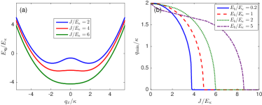
Figure 1: Two-body bound state. (a) The bound state energy $E_{\mathbf{q}}$ as a function of COM momentum $\mathbf{q}=q_{x}\hat{e}_{x}$ at $E_{b}/E_{\kappa}=1$, for $J/E_{\kappa}=2$, 4, and 6. (b) The ground-state momentum of the bound state as a function of the tunneling strength $J$ for atomic interaction $E_{b}/E_{\kappa}=0.2$, 1, 2, and 5. The energy and momentum are measured in units of $E_{\kappa}=\kappa^{2}/2$ and $\kappa$, respectively.

III Results

III.1 Two-body Problem

Since the pseudospin SOC does not mix the spin singlet and spin triplet, the wave function of two-body bound states can be constructed in the singlet space as

$$|\Phi\rangle_{\mathbf{q}}=\frac{1}{2}\sum_{\mathbf{k}}\sum_{j,l=1}^{2}\phi_{\mathbf{k}\mathbf{q},jl}S_{\mathbf{k}\mathbf{q},jl}^{{\dagger}}\left|0\right\rangle,$$ (3)

with

$$S_{\mathbf{k}\mathbf{q},jl}^{{\dagger}}=\frac{1}{\sqrt{2}}[\psi_{j\uparrow}^{{\dagger}}(\mathbf{Q}_{+})\psi_{l\downarrow}^{{\dagger}}(\mathbf{Q}_{-})-\psi_{j\downarrow}^{{\dagger}}(\mathbf{Q}_{+})\psi_{l\uparrow}^{{\dagger}}(\mathbf{Q}_{-})]$$ (4)

and $\mathbf{Q}_{\pm}=\mathbf{q}/2\pm\mathbf{k}$. Here $S_{\mathbf{qk},jl}^{{\dagger}}$ is a singlet operator for creating a pair of atoms in the layers $j$ and $l$ with a center-of-mass (COM) momentum $\mathbf{q}$ and a relative momentum $\mathbf{k}$, and $\phi_{\mathbf{k}\mathbf{q},jl}$ is the corresponding amplitude. For $j=l$ the atoms are paired in the same layer, whereas for $j\neq l$ the pairing takes place in different layers, the latter contribution emerging due to the laser-assisted tunneling. Since $S_{-\mathbf{k}\mathbf{q},jl}^{{\dagger}}=S_{\mathbf{k}\mathbf{q},lj}^{{\dagger}}$, we take $\phi_{-\mathbf{k}\mathbf{q},jl}=\phi_{\mathbf{k}\mathbf{q},lj}$ in Eq. (3), in which the factor $1/2$ is to avoid a double counting of the atomic pair states. Substituting Eq. (3) into the stationary Schrödinger equation $\mathcal{H}|\Phi\rangle_{\mathbf{q}}=E_{\mathbf{q}}|\Phi\rangle_{\mathbf{q}}$, one arrives at the following equation for the bound state energy $E_{\mathbf{q}}$ (see Appendix for details).

$$(\frac{U}{S}\sum_{\mathbf{k}}\frac{\alpha_{\mathbf{k}}}{\alpha_{\mathbf{k}}\gamma_{\mathbf{k}}-\beta_{\mathbf{k}}^{2}}-1)(\frac{U}{S}\sum_{\mathbf{k}}\frac{\gamma_{\mathbf{k}}}{\alpha_{\mathbf{k}}\gamma_{\mathbf{k}}-\beta_{\mathbf{k}}^{2}}-1)$$

$$-(\frac{U}{S}\sum_{\mathbf{k}}\frac{\beta_{\mathbf{k}}}{\alpha_{\mathbf{k}}\gamma_{\mathbf{k}}-\beta_{\mathbf{k}}^{2}})^{2}=0\,,$$ (5)

where $\alpha_{\mathbf{k}}=E_{\mathbf{q}}-(\mathbf{k}^{2}+\mathbf{q}^{2}/4+\kappa^{2})$, $\beta_{\mathbf{k}}=q_{x}\kappa$ and $\gamma_{\mathbf{k}}=\alpha_{\mathbf{k}}-\{\frac{J^{2}/2}{\alpha_{\mathbf{k}}+2k_{x}\kappa}+\frac{J^{2}/2}{\alpha_{\mathbf{k}}-2k_{x}\kappa}\}$. By solving Eq. (5) we can determine $E_{\mathbf{q}}$ as a function of the COM momentum.

Figure 1a illustrates that two degenerate minima are formed at $\mathbf{q}_{0}=\pm q_{{\rm min}}\mathbf{e}_{x}$ in the bound state energy spectrum $E_{\mathbf{q}}$. This is in sharp contrast to the SOC for real spins, where the bound state always has a zero COM momentum, or a single finite momentum if an in-plane Zeeman field is applied to break the SI symmetry Dong2013PRA . Furthermore, the interlayer singlet component $P_{12}=\sum_{\mathbf{k}}|\phi_{\mathbf{k}\mathbf{q},12}|^{2}$ is enhanced as the tunneling strength $J$ increases. Figure 1b shows the numerical result of the minimal momentum $q_{{\rm min}}=|\mathbf{q}_{0}|$ versus $J$ for the bound state. In the strong tunneling limit where the tunneling strength exceeds a critical value $J>J_{c}$, a bound state with zero momentum is eventually formed. On the other hand, we note that the critical tunneling $J_{c}$ increases with $E_{b}$, showing that increasing intralayer interaction enhances the formation of bound state with finite-momentum.

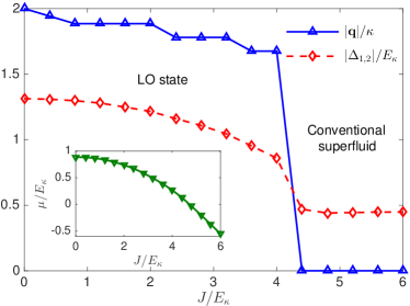
Figure 2: Pairing orders of superfluid phases. Dependence of $|\Delta_{1,2}|$ (red dashed) and the pairing momentum $|\mathbf{q}|$ (blue solid) on the tunneling strength $J$, where $|\Delta_{1,2}|$ represents the maximum value of the order parameter $|\Delta_{1,2}(x,y)|$ in the $xy$ plane. The inset shows the evolution of the chemical potential $\mu$. In the simulations, we have included a weak harmonic trap with frequency $\omega\ll E_{\kappa}$, $R_{\rm TF}\equiv\sqrt{2E_{\kappa}/m\omega^{2}}=\kappa/\omega$, $E_{b}/E_{\kappa}=1$, and $E_{F}\sim E_{\kappa}$.

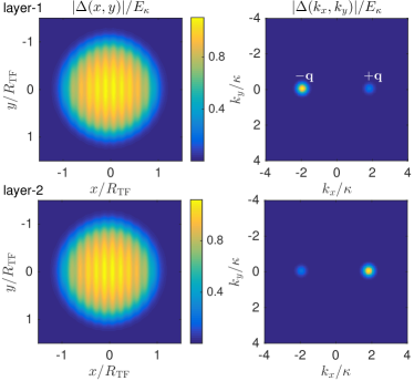
Figure 3: The density profile of the LO order parameter. Real-space density profile (left panel) and momentum space distribution (right panel) of the superfluid order parameters $\Delta_{1,2}$ for $J/E_{\kappa}=2$, where two pairing peaks with opposite momenta $\pm\mathbf{q}$ can be identified in each layer. In the simulations, we have included a weak harmonic trap with frequency $\omega\ll E_{\kappa}$, $R_{\rm TF}\equiv\sqrt{2E_{\kappa}/m\omega^{2}}=\kappa/\omega$, $E_{b}/E_{\kappa}=1$, and $E_{F}\sim E_{\kappa}$.

III.2 Phase Diagram of Superfluidity

We proceed to study the superfluid phase by computing the real-space superfluid order parameters $\Delta_{j}(\mathbf{r})=-U\langle\hat{\psi}_{j,\downarrow}(\mathbf{r})\hat{\psi}_{j,\uparrow}(\mathbf{r})\rangle$ for the layers $j=1,2$, and determine the ground state by solving the Bogoliubov-de Gennes (BdG) equation $H_{{\rm BdG}}(\mathbf{r})\phi_{\eta}=\varepsilon_{\eta}\phi_{\eta}$, where $H_{{\rm BdG}}$ is a $8\times 8$ matrix, $\phi_{\eta}$ represents the Nambu basis, and $\varepsilon_{\eta}$ is the corresponding energy of the Bogoliubov quasiparticles labeled by an index $\eta$ (see Appendix for the explicit form). The Fourier transformation of the superfluid order parameters $\Delta_{j}(\mathbf{r})=\sum_{\mathbf{q}}\Delta_{\mathbf{q}}e^{i\mathbf{q}\cdot\mathbf{r}}$ yields different situations. When $\Delta_{\mathbf{q}}\neq 0$ for $\mathbf{q}\neq 0$, the system represents a finite-momentum superfluid. When $\Delta_{\mathbf{q}}\neq 0$ for $\mathbf{q}=0$, the system is in a conventional superfluid phase. Otherwise, the system is in a normal state.

Figure 2 illustrates a behavior of the order parameter $|\Delta_{1,2}|$ and the pairing momentum $|\mathbf{q}|$ as functions of the tunneling strength $J$. One can see that by increasing $J$, the pairing momentum $|\mathbf{q}|$ decreases gradually and eventually vanishes at a critical value of the tunneling strength $\sim 4.3E_{\kappa}$. This defines a transition from the finite-momentum pairing state to the conventional superfluid characterized by a zero pairing momentum. Across the transition, the chemical potential $\mu$ decreases continuously, as shown in the inset of Fig. 2.

In Fig. 3, we present a density profile of the order parameter at a moderate tunneling $J/E_{\kappa}=2$. One can find that the system is in a superfluid phase with the order parameter $\Delta_{1,2}$ exhibiting an obvious density-modulation in the real-space profile (left panel of Fig. 3). The corresponding momentum distributions of $|\Delta_{1,2}|$ are shown in the right panel of Fig. 3. Interestingly, a pair of peaks with opposite momenta $\pm\mathbf{q}\sim\pm 1.9\kappa\mathbf{e}_{x}$ can be identified in each layer, so the pairing order parameter contains both momentum components $\Delta_{j}\sim c_{j}e^{-i\mathbf{q}\cdot\mathbf{x}}+d_{j}e^{i\mathbf{q}\cdot\mathbf{x}}$, with $c_{j}$ and $d_{j}$ being the corresponding amplitudes. This results in the spatial modulation of the order parameter with the periodicity $2\pi/|\mathbf{q}|$. In this way, the LO superfluid state is formed which breaks the translational symmetry and exhibits supersolid properties. Note that the density-modulation of the pairing order parameter is gauge invariant. In fact, transforming back to the laboratory frame ($\tilde{\psi}_{\gamma 1}=e^{i\kappa x}\psi_{\gamma 1}$ and $\tilde{\psi}_{\gamma 2}=e^{-i\kappa x}\psi_{\gamma 2}$), the order parameter $\tilde{\Delta}_{j}\equiv-U\langle\tilde{\psi}_{j\downarrow}\tilde{\psi}_{j\uparrow}\rangle=e^{\pm i2\kappa x}\Delta_{j}$ acquires only a phase factor $e^{\pm i2\kappa x}$, so the density modulation is unchanged.

The broad parameter regime shown for the LO phase reflects the essential difference between the present pseudospin SOC system and the real SOC Fermi gases, which can be understood in the following way. In a 1D SOC system the spin-up and spin-down pockets of the dispersion are shifted with respect to each other due to the momentum transfer between spin-up and spin-down states induced by the Raman coupling. The Raman coupling also opens a gap in the band crossing between spin-up and spin-down pockets at zero momentum Liu2009PRL ; Lin2011Nature . In the presence of an attractive $s$-wave interaction, the favored superfluid pairing occurs between spin-up and spin-down states with opposite momenta, respectively in the left-well and right-well pockets of the Fermi surface, leading to the conventional BCS state. The LO state can be realized only when the pairing within each (left-well/right-well) pocket is dominated. This can be in principle achieved by considering an attractive $p$-wave interaction which, however, is currently a major challenge in cold atom experiments.

In comparison, in the present pseudospin SOC system, the left and right pockets of the double-well dispersion shown in Fig. 4(a,b) correspond to predominantly opposite pseudospin (i.e. layer) states $|1^{\prime}\rangle$ and $|2^{\prime}\rangle$, while the interlayer tunneling can mix the pseudospin-up and -down states [Fig. 4(b)]. From the above analysis one can soon realize that the LO phase may be realized if there is an attractive $p$-wave like interaction in the pseudospin space, which induces pairings within each pocket of the Fermi surface. As explained below, such an effective $p$-wave like interaction arises naturally in the present bilayer system with the intralayer $s$-wave interaction.

Figure 4: The phase diagram. (a) Single-particle spectrum of the bilayer system for $J/E_{\kappa}=2$. The red solid line denotes the value of $E_{F}$ ($\sim E_{\kappa}$) in the simulations. (b) Topology of the Fermi surface when the Fermi level is situated in the lower dispersion branch, the gap, and the upper branch. The color bar represents the pseudospin polarizations $P_{\mathbf{k}}=\frac{\langle\hat{n}_{1\mathbf{k}}\rangle-\langle\hat{n}_{2\mathbf{k}}\rangle}{\langle\hat{n}_{1\mathbf{k}}\rangle+\langle\hat{n}_{2\mathbf{k}}\rangle}$. (c) Phase diagram of superfluidity in the $J-E_{b}$ plane with $E_{F}\sim E_{\kappa}$. The LO phase is obtained in a very broad parameter regime.

Considering the intralayer atomic interaction $\sim U\int d\mathbf{r}\sum_{j}\hat{n}_{j\downarrow}(\mathbf{r})\hat{n}_{j\uparrow}(\mathbf{r})$, let us treat the layer states ($j=1,2$) as fictitious spin states: $j\rightarrow s=\Uparrow,\Downarrow$. In turn, we treat the real spin states ($\gamma=\uparrow,\downarrow$) as an artificial spatial degree of freedom (e.g. $s$ and $p$ orbital states) denoted by $A$ and $B$. With these notations, the intralayer atomic interaction $\sim U\int d\mathbf{r}\sum_{s=\Uparrow,\Downarrow}\hat{n}_{s,A}(\mathbf{r})\hat{n}_{s,B}(\mathbf{r})$ describes an effective $p$-wave interaction between the atoms with different “orbits” $A$ and $B$ and the same “spin” $s$. This is essentially the underlying mechanism for the realization of the LO phase in a very broad parameter range, as one can see in Fig. 4c which shows the phase diagram in the $J-E_{b}$ plane. Note that the very broad LO phase has been obtained for all different Fermi energies $E_{F}$ depicted with dashed lines in Fig. 4a.

The BCS-BEC crossover can be achieved by tuning the binding energy $E_{b}$ for the present bilayer pseudospin SOC system. This is different from the Fermi gases with a 2D Rashba-type SOC in real spin space, where the BCS-BEC crossover can be achieved by tuning the Raman recoil energy across the regime that $E_{F}\sim E_{\kappa}$, with the BEC of rashbons being obtained when $E_{\kappa}>E_{F}$ Hu2011PRL ; Yu2011PRL ; Shenoy2013JPB . Note that $E_{b}$ is closely related to the 3D $s$-wave scattering length via $E_{b}=\frac{\mathcal{C}\omega_{z}}{\pi}e^{\sqrt{2}\pi l_{z}/a_{s}}$, with $\omega_{z}$ and $l_{z}$ being the frequency and length of the axial trapping perpendicular to the 2D plane Petrov . In the BCS regime one has $E_{b}/E_{F}\ll 1$, and the opposite holds in the BEC regime with $E_{b}/E_{F}\gg 1$. In Fig. 4c we take $E_{\kappa}\sim E_{F}$ so that $E_{b}/E_{\kappa}\sim E_{b}/E_{F}$, and the BCS-BEC crossover with spatial modulations is clearly obtained.

The present results reveal a profound connection between the LO state of fermions and the stripe phase of bosons. In the BEC regime with large $E_{b}$ limit, where $E_{b}/E_{F}\gg 1$, all atoms get paired to tight dimers in each layer. In this situation, the effective tunneling $\tilde{J}\sim J^{2}/\epsilon_{B}$ of the dimers with the momentum shift $\pm\tilde{\kappa}\sim\pm 2\kappa$ can induce the interference of the dimers between the two layers, rendering a stripe-type phase of the dimer BECs, where $\epsilon_{B}$ is a binding energy of the dimer state in the presence of pseudospin SOC. On the other hand, in the BCS regime with weak pairing condition, the atoms are loosely paired on the Fermi surface, and the fermionic nature of the atoms plays the important role. The momentum shift in the tunneling of individual atoms dominates the spatial modulation of the effective $p$-wave pairing order, leading to formation of the fermionic supersolidity of LO state and the superfluid phase transition, as shown in Fig. 4c.

IV Discussion and Conclusion

In the real experiment, the bilayer geometry for ultracold atoms can be implemented using a double-well superlattice potential which forms a stack of weakly coupled bilayer systems and has already realized in experiment for bosons Li2017Nature . The multiple bilayer configuration can enhance the superfluid transition Orso and increase the signal-to-noise ratio. Note that the typical pairing momentum $|\mathbf{q}|$ is on the order of the laser recoil $\kappa$. The corresponding spatial modulation of the LO state can be readily detected by the optical Brag scattering Li2017Nature .

In conclusion, we have proposed a highly feasible way to realize the LO phase in the bilayer Fermi gases with both the TR and SI symmetries. The laser-assisted tunneling between layers, which generates a 1D pseudospin SOC, is applied to induce the relative momentum shift between pairing orders in the bilayer Fermi gas, leading to the spontaneous formation of LO phase. The realization of the LO phase is also rooted in a novel mechanism that the intralayer $s$-wave attractive interaction combined with the pseudospin SOC renders an effective $p$-wave pairing phase in the pseudospin space. With the system preserving both TR and SI symmetries, the LO phase has been predicted in a very broad parameter regime. This work paves the way to realize the LO phase within the current experimental accessibility.

V acknowledgement

We thank Joachim Brand, Wolfgang Ketterle, Ana Maria Rey, and Gora Shlyannikov for helpful discussions and useful suggestions. This work is supported by the NSFC under Grants No. 11875195, No. 11404225, No. 11474205, and No. 11504037. Q. Sun, A.-C. Ji and X.-J Liu also acknowledge the support by the foundation of Beijing Education Committees under Grants No. CIT&TCD201804074, No. KM201510028005, No. KZ201810028043, and the support from the National Key R&D Program of China (2016YFA0301604), NSFC (No. 11574008 and No. 11761161003), and by the Strategic Priority Research Program of Chinese Academy of Science (Grant No. XDB28000000).

Appendix A Derivation of the Hamiltonian

We consider a two-component Fermi gas composed of atoms in two metastable internal (quasi-spin) states labeled by the index $\gamma=\uparrow,\downarrow$, as shown in Fig. 5. The atoms are confined in a state-independent double-well optical potential along the $z$-axis providing a bilayer structure. As in ref. Li2016PRL , we assume an asymmetry of the double-well potential preventing a direct atomic tunneling between the wells, and instead two Raman lasers are applied to induce a laser-assisted interlayer tunneling. In the laboratory frame, the single particle Hamiltonian for each component is

$$H_{\gamma}=\int d^{2}\mathbf{r}\left\{\sum_{j=1,2}\tilde{\psi}^{\dagger}_{\gamma j}(\mathbf{r})\left[\frac{\mathbf{P}^{2}}{2m}+(-1)^{j}\frac{h}{2}\pm\frac{\delta}{2}\right]\tilde{\psi}_{\gamma j}(\mathbf{r})+\left(\frac{J}{2}e^{i2\hbar\kappa\mathbf{e}_{x}\cdot\mathbf{r}}\tilde{\psi}^{\dagger}_{\gamma 1}(\mathbf{r})\tilde{\psi}_{\gamma 2}(\mathbf{r})+h.c.\right)\right\},$$ (6)

where the upper and lower signs correspond to different atomic internal states $\gamma$, and $\mathbf{P}$ and $m$ are the momentum and mass of the atom respectively. $\tilde{\psi}_{\gamma j}(\mathbf{r})$ annihilates a Fermi atom at position $\mathbf{r}$ in the $j$-th layer with an internal state $\gamma$. $J$ is a strength of the laser-assisted interlayer tunneling with $2\hbar\kappa$ being an associated recoil momentum along the $x$-direction. $h$ and $\delta$ denote the energy mismatch between the two layers and two components. Note that, both spin components are characterized by the same laser-assisted tunneling. In writing Eq.(6) we have neglected the off-resonant transition by applying the Rotating Wave Approximation (RWA) for the laser-assisted interlayer tunneling.

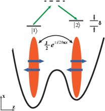
Figure 5: Illustrative sketch of the system. A two-component Fermi gas composed of atoms in two metastable internal (spin) states are confined in a state-independent double-well optical potential along the $z$-axis. An asymmetry of the double-well potential prevents a direct atomic tunneling between the wells, and instead two Raman lasers are applied to induce a laser-assisted interlayer tunneling. Here, $J$ is a strength of the laser-assisted interlayer tunneling with $2\hbar\kappa$ being an associated recoil momentum along the $x$-direction, $\delta$ denotes the energy mismatch between the two layer states.

In terms of $\tilde{\psi}_{\gamma j}(\mathbf{r})$, the atom-atom coupling described by the contact interaction between the fermions within individual layers in different internal states $\gamma$ can be written as

$$H_{\rm int}=\frac{U}{2}\sum_{\gamma,j}\int d^{2}\mathbf{r}\tilde{\psi}^{\dagger}_{\gamma j}(\mathbf{r})\tilde{\psi}_{\gamma j}(\mathbf{r})\tilde{\psi}^{\dagger}_{\bar{\gamma}j}(\mathbf{r})\tilde{\psi}_{\bar{\gamma}j}(\mathbf{r}).$$ (7)

with $U$ the contact interaction strength in two dimension.

We now apply a gauge transformation $\psi_{\gamma 1}=e^{-i\hbar\kappa\mathbf{e}_{x}\cdot\mathbf{r}}\tilde{\psi}_{\gamma 1}$ and $\psi_{\gamma 2}=e^{i\hbar\kappa\mathbf{e}_{x}\cdot\mathbf{r}}\tilde{\psi}_{\gamma 2}$. Then, Hamiltonian (6) becomes

$$H_{\gamma}=\int d^{2}\mathbf{r}\left\{\sum_{j=1,2}\psi^{\dagger}_{\gamma j}(\mathbf{r})\left[\frac{\mathbf{(P+(-1)^{j+1}\hbar\kappa}\mathbf{e}_{x})^{2}}{2m}+(-1)^{j}\frac{h}{2}\pm\frac{\delta}{2}\right]\psi_{\gamma j}(\mathbf{r})+\frac{J}{2}\left(\psi^{\dagger}_{\gamma 1}(\mathbf{r})\psi_{\gamma 2}(\mathbf{r})+h.c.\right)\right\},$$ (8)

while the form of the interaction Hamiltonian, Eq. (7), is unchanged. By making use of the Fourier transformation $\psi_{\gamma j}(\mathbf{r})=\frac{1}{\sqrt{S}}\sum_{\mathbf{k}}\psi_{\gamma j}(\mathbf{k})e^{i\hbar\mathbf{k}\cdot\mathbf{r}}$ and setting $\hbar$ to the unity, we obtain the the momentum space Hamiltonian given by Eq.(1) in the main text.

Appendix B Two-body bound state

Let us begin with the two-body problem, which helps to intuitively understand the many-body behavior of this system. The molecular state with center-of-mass (COM) momentum $\mathbf{q}$ can be constructed as $|\Phi\rangle_{\mathbf{q}}=\frac{1}{2}\sum_{\mathbf{k}}\sum_{j,l=1}^{2}\phi_{\mathbf{k}\mathbf{q},jl}S_{\mathbf{k}\mathbf{q},jl}^{{\dagger}}\left|0\right\rangle$ with

$$S_{\mathbf{k}\mathbf{q},jl}^{{\dagger}}=\frac{1}{\sqrt{2}}[\psi_{j\uparrow}^{{\dagger}}(\mathbf{Q}_{+})\psi_{l\downarrow}^{{\dagger}}(\mathbf{Q}_{-})-\psi_{j\downarrow}^{{\dagger}}(\mathbf{Q}_{+})\psi_{l\uparrow}^{{\dagger}}(\mathbf{Q}_{-})],$$ (9)

where $\mathbf{Q}_{\pm}=\mathbf{q}/2\pm\mathbf{k}$ and $S_{\mathbf{qk},jl}^{{\dagger}}$ is a singlet operator for creating a pair of atoms in the layers $j$ and $l$ with a COM momentum $\mathbf{q}$ and a relative momentum $\mathbf{k}$, and $\phi_{\mathbf{k}\mathbf{q},jl}$ is the corresponding probability amplitude. Here, we have used the fact that the four singlet operators introduced above form an invariant subspace of the total Hamiltonian $\mathcal{H}$ and hence serve as a complete basis for the bound state. Notice that due to relations $S_{-\mathbf{k}\mathbf{q},jl}^{{\dagger}}=S_{\mathbf{k}\mathbf{q},lj}^{{\dagger}}$ and $\phi_{-\mathbf{k}\mathbf{q},jl}=\phi_{\mathbf{k}\mathbf{q},lj}$, we have added a factor $1/2$ in the summations $\sum_{\mathbf{k}}$ to avoid a double counting of the terms comprising the state vector $|\Phi\rangle_{\mathbf{q}}$.

Substituting the wave-function $|\Phi\rangle_{\mathbf{q}}$ into the stationary Schrödinger equation $\mathcal{H}|\Phi\rangle_{\mathbf{q}}=E_{\mathbf{q}}|\Phi\rangle_{\mathbf{q}}$ one can get the following explicit form for each component:

$$E_{\mathbf{q}}\phi_{\mathbf{kq},11} = \{\mathbf{k}^{2}+(\mathbf{q}/2+\kappa\mathbf{e}_{x})^{2}-h\}\phi_{\mathbf{kq},11}+\frac{J}{2}(\phi_{\mathbf{kq},12}+\phi_{\mathbf{kq},21})+\frac{U}{S}\sum_{\mathbf{k}^{\prime}}\phi_{\mathbf{k^{\prime}q},11}$$ (10)

$$E_{\mathbf{q}}\phi_{\mathbf{kq},12} = \{(\mathbf{k}+\kappa\mathbf{e}_{x})^{2}+\mathbf{q}^{2}/4\}\phi_{\mathbf{kq},12}+\frac{J}{2}(\phi_{\mathbf{kq},11}+\phi_{\mathbf{kq},22})$$ (11)

$$E_{\mathbf{q}}\phi_{\mathbf{kq},21} = \{(\mathbf{k}-\kappa\mathbf{e}_{x})^{2}+\mathbf{q}^{2}/4\}\phi_{\mathbf{kq},21}+\frac{J}{2}(\phi_{\mathbf{kq},11}+\phi_{\mathbf{kq},22})$$ (12)

$$E_{\mathbf{q}}\phi_{\mathbf{kq},22} = \{\mathbf{k}^{2}+(\mathbf{q}/2-\kappa\mathbf{e}_{x})^{2}+h\}\phi_{\mathbf{kq},22}+\frac{J}{2}(\phi_{\mathbf{kq},12}+\phi_{\mathbf{kq},21})+\frac{U}{S}\sum_{\mathbf{k}^{\prime}}\phi_{\mathbf{k^{\prime}q},22}.$$ (13)

where $E_{\mathbf{q}}$ is an eigenenergy. Then, we have

$$E_{\mathbf{q}}(\phi_{\mathbf{kq},11}+\phi_{\mathbf{kq},22}) = (\mathbf{k}^{2}+\mathbf{q}^{2}/4+\kappa^{2})(\phi_{\mathbf{kq},11}+\phi_{\mathbf{kq},22})+(q_{x}\kappa-h)(\phi_{\mathbf{kq},11}-\phi_{\mathbf{kq},22})$$ (14)

$$+ \Omega(\phi_{\mathbf{kq},12}+\phi_{\mathbf{kq},21})+\frac{U}{S}\sum_{\mathbf{k}^{\prime}}(\phi_{\mathbf{k^{\prime}q},11}+\phi_{\mathbf{k^{\prime}q},22})$$ (15)

$$E_{\mathbf{q}}(\phi_{\mathbf{kq},11}-\phi_{\mathbf{kq},22}) = (\mathbf{k}^{2}+\mathbf{q}^{2}/4+\kappa^{2})(\phi_{\mathbf{kq},11}-\phi_{\mathbf{kq},22})+(q_{x}\kappa-h)(\phi_{\mathbf{kq},11}+\phi_{\mathbf{kq},22})$$ (16)

$$+ \frac{U}{S}\sum_{\mathbf{k}^{\prime}}(\phi_{\mathbf{k^{\prime}q},11}-\phi_{\mathbf{k^{\prime}q},22})$$ (17)

$$(\phi_{\mathbf{kq},12}+\phi_{\mathbf{kq},21}) = \left\{\frac{J/2}{E_{\mathbf{q}}-(\mathbf{k}+\kappa\mathbf{e}_{x})^{2}-\mathbf{q}^{2}/4}+\frac{J/2}{E_{\mathbf{Q}}-(\mathbf{k}-\kappa\mathbf{e}_{x})^{2}-\mathbf{q}^{2}/4}\right\}(\phi_{\mathbf{kq},11}+\phi_{\mathbf{kq},22}).$$ (18)

Solving the above equations, one finds

$$(\phi_{\mathbf{kq},11}+\phi_{\mathbf{kq},22})=\frac{\gamma_{\mathbf{k}}\frac{U}{S}\sum_{\mathbf{k}^{\prime}}(\phi_{\mathbf{k^{\prime}q},11}+\phi_{\mathbf{k^{\prime}q},22})+\beta_{\mathbf{k}}\frac{U}{S}\sum_{\mathbf{k}^{\prime}}(\phi_{\mathbf{k}^{\prime},1}-\phi_{\mathbf{k}^{\prime},4})}{\alpha_{\mathbf{k}}\gamma_{\mathbf{k}}-\beta_{\mathbf{k}}^{2}}$$ (19)

$$(\phi_{\mathbf{kq},11}-\phi_{\mathbf{kq},22})=\frac{\alpha_{\mathbf{k}}\frac{U}{S}\sum_{\mathbf{k}^{\prime}}(\phi_{\mathbf{k^{\prime}q},11}-\phi_{\mathbf{k^{\prime}q},22})+\beta_{\mathbf{k}}\frac{U}{S}\sum_{\mathbf{k}^{\prime}}(\phi_{\mathbf{k^{\prime}q},11}+\phi_{\mathbf{k^{\prime}q},22})}{\alpha_{\mathbf{k}}\gamma_{\mathbf{k}}-\beta_{\mathbf{k}}^{2}},$$ (20)

with $\alpha_{\mathbf{k}}=E_{\mathbf{q}}-(\mathbf{k}^{2}+\mathbf{q}^{2}/4+\kappa^{2})$, $\beta_{\mathbf{k}}=q_{x}\kappa-h$, and $\gamma_{\mathbf{k}}=\alpha_{\mathbf{k}}-\left\{\frac{J^{2}/2}{E_{\mathbf{q}}-(\mathbf{k}+\kappa\mathbf{e}_{x})^{2}-\mathbf{q}^{2}/4}+\frac{J^{2}/2}{E_{\mathbf{q}}-(\mathbf{k}-\kappa\mathbf{e}_{x})^{2}-\mathbf{q}^{2}/4}\right\}$.

After some straightforward derivations, we arrive at the following self-consistent equation for the molecular energy $E_{\mathbf{q}}$:

$$(\frac{U}{S}\sum_{\mathbf{k}}\frac{\alpha_{\mathbf{k}}}{\alpha_{\mathbf{k}}\gamma_{\mathbf{k}}-\beta_{\mathbf{k}}^{2}}-1)(\frac{U}{S}\sum_{\mathbf{k}}\frac{\gamma_{\mathbf{k}}}{\alpha_{\mathbf{k}}\gamma_{\mathbf{k}}-\beta_{\mathbf{k}}^{2}}-1)-(\frac{U}{S}\sum_{\mathbf{k}}\frac{\beta_{\mathbf{k}}}{\alpha_{\mathbf{k}}\gamma_{\mathbf{k}}-\beta_{\mathbf{k}}^{2}})^{2}=0.$$ (21)

Notice that, $\alpha_{\mathbf{k}}$, $\beta_{\mathbf{k}}$ and $\gamma_{\mathbf{k}}$ do not depend on the detuning $\delta$ between two components, i.e. the two-body spectrum obtained using Eq. (21) would not be altered by changing $\delta$. On the other hand, the detuning shifts the single particle spectrum by $\pm\delta/2$ for different spin components.

Minimizing $E_{\mathbf{q}}$ with respect to the COM momentum $\mathbf{q}$, one can obtain the ground state energy of the molecular state. The corresponding coefficients $\phi_{\mathbf{kq},jl}$ (not normalized) are given by

$$\sum_{\mathbf{k}^{\prime}}(\phi_{\mathbf{k^{\prime}q},11}-\phi_{\mathbf{k^{\prime}q},22}) = \sum_{\mathbf{k}^{\prime}}(\phi_{\mathbf{k^{\prime}q},11}+\phi_{\mathbf{k^{\prime}q},22})(\frac{U}{S}\sum_{\mathbf{k}}\frac{-\beta_{\mathbf{k}}}{\alpha_{\mathbf{k}}\gamma_{\mathbf{k}}-\beta_{\mathbf{k}}^{2}})/(\frac{U}{S}\sum_{\mathbf{k}}\frac{\alpha_{\mathbf{k}}}{\alpha_{\mathbf{k}}\gamma_{\mathbf{k}}-\beta_{\mathbf{k}}^{2}}-1)$$ (22)

$$(\phi_{\mathbf{kq},11}+\phi_{\mathbf{kq},22}) = \frac{\gamma_{\mathbf{k}}\frac{U}{S}\sum_{\mathbf{k}^{\prime}}(\phi_{\mathbf{k^{\prime}q},11}+\phi_{\mathbf{k^{\prime}q},22})+\beta_{\mathbf{k}}\frac{U}{S}\sum_{\mathbf{k}^{\prime}}(\phi_{\mathbf{k^{\prime}q},11}-\phi_{\mathbf{k^{\prime}q},22})}{\alpha_{\mathbf{k}}\gamma_{\mathbf{k}}-\beta_{\mathbf{k}}^{2}}$$ (23)

$$(\phi_{\mathbf{kq},11}-\phi_{\mathbf{kq},22}) = \frac{\alpha_{\mathbf{k}}\frac{U}{S}\sum_{\mathbf{k}^{\prime}}(\phi_{\mathbf{k^{\prime}q},11}-\phi_{\mathbf{k^{\prime}q},22})+\beta_{\mathbf{k}}\frac{U}{S}\sum_{\mathbf{k}^{\prime}}(\phi_{\mathbf{k^{\prime}q},11}+\phi_{\mathbf{k^{\prime}q},22})}{\alpha_{\mathbf{k}}\gamma_{\mathbf{k}}-\beta_{\mathbf{k}}^{2}}$$ (24)

$$\phi_{\mathbf{kq},12} = \frac{J/2}{E_{\mathbf{q}}-(\mathbf{k}+\kappa\mathbf{e}_{x})^{2}-\mathbf{q}^{2}/4}(\phi_{\mathbf{kq},11}+\phi_{\mathbf{kq},22})$$ (25)

$$\phi_{\mathbf{kq},21} = \frac{J/2}{E_{\mathbf{q}}-(\mathbf{k}-\kappa\mathbf{e}_{x})^{2}-\mathbf{q}^{2}/4}(\phi_{\mathbf{kq},11}+\phi_{\mathbf{kq},22}).$$ (26)

For vanishing interlayer and intercomponent detunings, i.e. $h=\delta=0$, one recovers the results in the main text. Some remarks: (i) For zero recoil $\kappa=0$, we have $\beta_{\mathbf{k}}=0$ and Eq. (21) reduces to $\frac{U}{S}\sum_{\mathbf{k}}\frac{1}{\alpha_{\mathbf{k}}}-1=0$ and $\frac{U}{S}\sum_{\mathbf{k}}\frac{1}{\gamma_{\mathbf{k}}}-1=0$, with the binding energy $E_{b}^{(1)}=\sqrt{E_{b}^{2}+J^{2}}-J$ and $E_{b}^{(2)}=E_{b}-J$ modified simply by the tunneling strength $J$. Compared with usual $E_{b}$, we see that the binding energies are modified simply by the tunneling strength $J$. (ii) For $J=0$, the momentum transfer $2\kappa\mathbf{e}_{x}$ brought by the Raman coupling can be simply gauged away via a unitary transformation describing the layer-dependent momentum shift, and the binding energy is $E_{b}^{(1)}=E_{b}^{(2)}=E_{b}$. (iii) For $\kappa\neq 0$ and $J\neq 0$, the attractive interaction between atoms in different internal states would act together with the interlayer tunneling and intra-component spin-orbit coupling. This can give rise to nontrivial two-body and many-body ground states discussed in the main text.

Appendix C Bogoliubov-de Gennes equation of the system

Since the atomic attraction takes place only in the same layer, we introduce the superfluid order parameters $\Delta_{j}(\textbf{r})=-U\left<\psi_{j,\downarrow}(\mathbf{r})\psi_{j,\uparrow}(\mathbf{r})\right>$ ($j=1,2$) with $\mathbf{r}=(x,y)$. Then, the Hamiltonian (1) in the main text can be diagonalized via a Bogoliubov–Valatin transformation. By taking into account an additional weak harmonic trapping potential $V(r)=m\omega^{2}r^{2}/2$, the resultant Bogoliubov-de Gennes (BdG) equation can be written as: $H_{\rm BdG}(\mathbf{r})\phi_{\eta}=\varepsilon_{\eta}\phi_{\eta}$. Here,

$$H_{\mathrm{BdG}}(\mathbf{r})=\left(\begin{matrix}H_{1}(\mathbf{r})&H_{J}\\ H^{\dagger}_{J}&H_{2}(\mathbf{r})\end{matrix}\right)\,$$ (27)

is an $8\times 8$ matrix with $H_{J}=\mathrm{diag}(J/2,J/2,-J/2,-J/2)$ describing the interlayer tunneling, and $H_{1,2}(\mathbf{r})$ denoting the single-particle Hamiltonian for each layer $j=1,2$. The latter $H_{j}(\mathbf{r})$ reads explicitly

$$\begin{split}H_{j}(\mathbf{r})&=\begin{pmatrix}\epsilon_{j\uparrow}(\mathbf{r})&0&0&-\Delta_{j}(\mathbf{r})\\ 0&\epsilon_{j\downarrow}(\mathbf{r})&\Delta_{j}(\mathbf{r})&0\\ 0&\Delta_{j}^{\ast}(\mathbf{r})&-\epsilon_{j\uparrow}^{\ast}(\mathbf{r})&0\\ -\Delta_{j}^{\ast}(\mathbf{r})&0&0&-\epsilon_{j\downarrow}^{\ast}(\mathbf{r})\\ \end{pmatrix}\,,\\ \end{split}$$ (28)

with $j=1,2$ and

$$\left\{\begin{aligned} \epsilon_{1\uparrow,\downarrow}(\mathbf{r})&=-\hbar^{2}\nabla^{2}/(2m)-i\hbar^{2}\kappa\partial_{x}/m+V(\mathbf{r})-\mu\\ \epsilon_{2\uparrow,\downarrow}(\mathbf{r})&=-\hbar^{2}\nabla^{2}/(2m)+i\hbar^{2}\kappa\partial_{x}/m+V(\mathbf{r})-\mu\\ \end{aligned}\right.\,.$$ (29)

Here, we have taken $h=\delta=0$. In this case, the ground state is spin balanced with equal chemical potential $\mu$ for both components. The Nambu basis is chosen as $\phi_{\eta}=[u_{1\uparrow,\eta},u_{1\downarrow,\eta},v_{1\uparrow,\eta},v_{1\downarrow,\eta},u_{2\uparrow,\eta},u_{2\downarrow,\eta},v_{2\uparrow,\eta},v_{2\downarrow,\eta}]^{T}$, and $\varepsilon_{\eta}$ is the corresponding energy of the Bogoliubov quasiparticles labeled by an index $\eta$. The order parameter $\Delta_{1,2}(\mathbf{r})$ is to be determined self-consistently by

$$\Delta_{j}(\mathbf{r})=-U\sum_{\eta}[u_{j\uparrow,\eta}v^{\ast}_{j\downarrow,\eta}f(-\varepsilon_{\eta})+u_{j\downarrow,\eta}v^{\ast}_{j\uparrow,\eta}f(\varepsilon_{\eta})]\,,$$

where $f(E)=1/[e^{E/k_{B}T}+1]$ is the Fermi-Dirac distribution function at a temperature $T$. The chemical potential $\mu$ is obtained using the number equation $N=\int d\mathbf{r}n(\mathbf{r})$, where the total atomic density is given by

$$n(\mathbf{r})=\sum_{j\gamma,\eta}[|u_{j\gamma,\eta}(\mathbf{r})|^{2}f(\varepsilon_{\eta})+|v_{j\gamma,\eta}(\mathbf{r})|^{2}f(-\varepsilon_{\eta})]\,.$$ (30)

The ground state can then be found by solving the above BdG equation self-consistently with the basis expansion method Xu2014PRL . In the numerical simulations, we have taken a large energy cutoff $\varepsilon_{c}=6E_{\mathrm{rec}}$ to ensure the accuracy of the calculation, where $E_{\mathrm{rec}}=5\hbar\omega$ assures that the trap oscillation frequency $\omega$ is much smaller than the recoil frequency.

References

• (1) P. Fulde, R. A. Ferrell, Phys. Rev. 135, A550 (1964).
• (2) A. I. Larkin, Y. N. Ovchinnikov, Zh. Eksp. Teor. Fiz. 47, 1136 (1964).
• (3) K. B. Gubbels, H. T. C. Stoof, Phys. Rep. 525, 255 (2012).
• (4) R. Casalbuoni, G. Nardulli, Rev. Mod. Phys. 76, 263 (2004).
• (5) R. Anglani, R. Casalbuoni, M. Ciminale, R. Gatto, N. Ippolito, M. Mannarelli, M. Ruggieri, Rev. Mod. Phys. 86, 509 (2014).
• (6) L. Radzihovsky, D. E Sheehy, Rep. Prog. Phys. 73, 076501 (2010).
• (7) M. Boninsegni, N. V. Prokof’ev, Rev. Mod. Phys. 84, 759 (2012).
• (8) J. Li, J. Lee, W. Huang, S. Burchesky, B. Shteynas, F. C. Top, A. O. Jamison, W. Ketterle, Nature 543, 91 (2017).
• (9) T. Mizushima, K. Machida, M. Ichioka, Phys. Rev. Lett. 94, 060404 (2005).
• (10) M. W. Zwierlein, A. Schirotzek, C. H. Schunck, W. Ketterle, Science 311, 492 (2006).
• (11) G. B. Partridge, W. Li, R. I. Kamar, Y. Liao, R. G. Hulet, Science 311, 503 (2006).
• (12) D. E. Sheehy, L. Radzihovsky, Phys. Rev. Lett. 96, 060401 (2006).
• (13) H. Hu, X.-J. Liu, Phys. Rev. A 73, 051603(R) (2006).
• (14) Y.-A. Liao, A. Rittner, T. Paprotta, W. Li, G. Partridge, R. Hulet, S. Baur, E. Mueller, Nature 467, 567 (2010).
• (15) Y.-J. Lin, K. Jiménez-García, I. B. Spielman, Nature 471, 83 (2011).
• (16) J.-Y. Zhang, S.-C. Ji, Z. Chen, L. Zhang, Z.-D. Du, B. Yan, G.-S. Pan, B. Zhao, Y.-J. Deng, H. Zhai, S. Chen, J.-W. Pan, Phys. Rev. Lett. 109, 115301 (2012).
• (17) P. J. Wang, Z.-Q. Yu, Z. K. Fu, J. Miao, L. H. Huang, S. J. Chai, H. Zhai, J. Zhang, Phys. Rev. Lett. 109, 095301 (2012).
• (18) L. W. Cheuk, A. T. Sommer, Z. Hadzibabic, T. Yefsah, W. S. Bakr, M. W. Zwierlein, Phys. Rev. Lett. 109, 095302 (2012).
• (19) C. Qu, C. Hamner, M. Gong, C. W. Zhang, P. Engels, Phys. Rev. A 88, 021604(R) (2013).
• (20) L. Huang, Z. Meng, P. Wang, P. Peng, S.-L. Zhang, L. Chen, D. Li, Q. Zhou, J. Zhang, Nat. Phys. 12, 540 (2016).
• (21) Z. Wu, L. Zhang, W. Sun, X.-T. Xu, B.-Z. Wang, S.-C. Ji, Y. Deng, S. Chen, X.-J. Liu, J.-W. Pan, Science 354, 83 (2016).
• (22) Z. Meng, L. Huang, P. Peng, D. Li, L. Chen, Y. Xu, C. Zhang, P. Wang, J. Zhang, Phys. Rev. Lett. 117, 235304 (2016).
• (23) V. Galitski, I. B. Spielman, Nature 494, 49 (2013).
• (24) N. Goldman, G. Juzeliūnas, P. Öhberg, I. B. Spielman, Rep. Prog. Phys. 77, 126401 (2014).
• (25) H. Zhai, Rep. Prog. Phys. 78, 026001(2015).
• (26) L. Zhang, X. -J. Liu, Synthetic spin-orbit coupling in cold atom (World Scientific, 2018), Chap. 1.
• (27) C. Chen, Phys. Rev. Lett. 111, 235302 (2013).
• (28) M. Iskin, A. L. Subasi, Phys. Rev. A 87, 063627 (2013).
• (29) X.-J. Liu, H. Hu, Phys. Rev. A 88, 023622 (2013).
• (30) F. Wu, G. C. Guo, W. Zhang, W. Yi, Phys. Rev. Lett. 110, 110401 (2013).
• (31) C. Qu, Z. Zheng, M. Gong, Y. Xu, L. Mao, X. Zou, G. Guo, C. Zhang, Nat. Commun. 4, 2710 (2013).
• (32) W. Zhang, W. Yi, Nat. Commun. 4, 2711 (2013).
• (33) L. Dong, L. Jiang, H. Hu, H. Pu, Phys. Rev. A 87, 043616 (2013).
• (34) Z. Zheng, M. Gong, X. Zou, C. Zhang, G. C. Guo, Phys. Rev. A 87, 031602(R) (2013).
• (35) Z. Zheng, C. Qu, X. Zou, C. Zhang, Phys. Rev. Lett. 116, 120403 (2016).
• (36) L. L. Wang, Q. Sun, W.-M. Liu, G. Juzeliūnas, An-Chun Ji, Phys. Rev. A 95, 053628 (2017).
• (37) T. -F. J. Poon, X.-J. Liu, Phys. Rev. B 97, 020501(R) (2018).
• (38) C. Chan, X.-J. Liu, Phys. Rev. Lett. 118, 207002 (2017).
• (39) C. Chan, L. Zhang, T.-F. J. Poon, Y.-P. He, Y.-Q. Wang, X.-J. Liu, Phys. Rev. Lett. 119, 047001 (2017).
• (40) J. Li, W. Huang, B. Shteynas, S. Burchesky, F. C. Top, E. Su, J. Lee, A. O. Jamison, W. Ketterle, Phys. Rev. Lett. 117, 185301 (2016).
• (41) Q. Sun, J. Hu, L. Wen, W.-M. Liu, G. Juzeliūnas, A.-C. Ji, Scientific Reports 6, 37679 (2016).
• (42) M. Randeria, J.-M. Duan, L.-Y. Shieh, Phys. Rev. Lett. 62, 981 (1989).
• (43) M. Randeria, J. M. Duan, L. Y. Shieh, Phys. Rev. B 41, 327 (1990).
• (44) X.-J. Liu, M. F. Borunda, X. Liu, J. Sinova, Phys. Rev. Lett. 102, 046402 (2009).
• (45) H. Hu, L. Jiang, X. J. Liu, H. Pu, Phys. Rev. Lett. 107, 195304 (2011).
• (46) Z. Q. Yu, H. Zhai, Phys. Rev. Lett. 107, 195305 (2011).
• (47) V. B Shenoy, J. P Vyasanakere, J. Phys. B 46, 134009 (2013).
• (48) D. S. Petrov, G. V. Shlyapnikov, Phys. Rev. A 64, 012706 (2001).
• (49) G. Orso, G. V. Shlyapnikov, Phys. Rev. Lett. 95, 260402 (2005).
• (50) Y. Xu, L. Mao, B. Wu, and C. Zhang, Phys. Rev. Lett. 113, 130404 (2014).