Scale-invariance and scale-breaking in parity-invariant three-dimensional QCD

Abstract

We present a numerical study of three-dimensional two-color QCD with $N=0,2,4,8$ and 12 flavors of massless two-component fermions using parity-preserving improved Wilson-Dirac fermions. A finite volume analysis provides strong evidence for the presence of $Sp(N)$ symmetry-breaking bilinear condensate when $N\leq 2$ and its absence for $N\geq 8$. A weaker evidence for the bilinear condensate is shown for $N=4$. We estimate the critical number of flavors below which scale-invariance is broken by the bilinear condensate to be between $N=4$ and 6.

I Introduction

Three-dimensional gauge theories coupled to an even number of two-component massless fermions can be regularized to form a parity-invariant theory. The parity-invariant fermion action for $N$ flavors of two-component fermions coupled to $SU(N_{c})$ gauge-field $A_{\mu}$ is

$$S_{f}=\int d^{3}x\sum_{i=1}^{N/2}\left\{\overline{\phi}_{i}(x)C(A)\phi_{i}(x)+\overline{\chi}_{i}(x)C^{\dagger}(A)\chi_{i}(x)\right\},$$ (1)

where $C(A)$ is the two-component Dirac operator, with an ultraviolet regularization being imposed implicitly. In the continuum,

$$C(A)=\sum_{\mu=1}^{3}\sigma_{\mu}(\partial_{\mu}+iA_{\mu}(x)),$$ (2)

with $\sigma_{\mu}$ being the three Pauli matrices. One can think of the above parity-invariant theory of $N$ flavors of two-component fermions to be equivalent to a theory of $\frac{N}{2}$ flavors of four-component fermions $\psi_{i}$ with a Hermitian Dirac operator $D$:

$$S_{f}=\sum_{i=1}^{N/2}\int d^{3}x\overline{\psi}_{i}(x)D\psi_{i}(x),$$ (3)

with the following identifications

$$\psi_{i}(x)=\begin{pmatrix}\phi_{i}(x)\\ \chi_{i}(x)\end{pmatrix};\quad\overline{\psi}_{i}(x)=(\overline{\chi}_{i}(x),\overline{\phi}_{i}(x));\quad D(A)=\begin{pmatrix}0&C^{\dagger}(A)\cr C(A)&0\end{pmatrix}.$$ (4)

Since $C^{\dagger}=-C$ in the continuum, the theory has a global $U(N)$ flavor symmetry. However, the $N_{c}=2$ theory is special, and there is a larger $Sp(N)$ global symmetry following from the property $\sigma_{2}\tau_{2}C\sigma_{2}\tau_{2}=C^{t}$, where $\sigma_{2}$ and $\tau_{2}$ are Pauli matrices in spin and color space respectively Magnea (2000). This is also related to the fact that the operator $D$ can be made real symmetric in a suitable basis Neuberger (1998).

Consider such a theory on an Euclidean periodic $l_{\rm ph}^{3}$ torus. Physics depends on the dimensionless size, $\ell=l_{\rm ph}g^{2}_{\rm ph}$, where $g^{2}_{\rm ph}$ is the physical coupling constant. Since $g^{2}_{\rm ph}$ has the dimension of mass, these theories are super-renormalizable, and the continuum limit in a lattice regularization at a fixed $\ell$ can be obtained by setting the lattice coupling constant (same as the lattice spacing) to $g^{2}_{\rm lat}=\frac{\ell}{L}$ on a periodic $L^{3}$ lattice and taking $L\to\infty$. The physics of this theory will smoothly cross-over from a non-interacting theory at small $\ell$ to a strongly interacting theory as $\ell\to\infty$; this strongly interacting theory could either be scale-invariant or scale-breaking. Scale-breaking is expected to produce a parity-preserving non-zero fermion bilinear condensate, that for a generic $SU(N_{c})$ gauge theory breaks the $U(N)$ flavor symmetry to $U\left(\frac{N}{2}\right)\times U\left(\frac{N}{2}\right)$ Pisarski (1984); Vafa and Witten (1984), but in the case of $SU(2)$ gauge theory breaks the $Sp(N)$ symmetry to $Sp\left(\frac{N}{2}\right)\times Sp\left(\frac{N}{2}\right)$ Magnea (2000). The possibility of the generation of any parity-breaking bilinear condensate has been argued against in Vafa and Witten (1984).

A numerical study of the Abelian $U(1)$ gauge theory using Wilson fermions showed no evidence for a bilinear condensate for any even value of $N>0$ Karthik and Narayanan (2016a). Since the Wilson fermions realize the $U(N)$ flavor symmetry only in the continuum limit, overlap fermions were used to study the theory with the symmetry present even away from the continuum. This enabled us to study the scale-invariant properties of the theory in further detail Karthik and Narayanan (2016b). Assuming the $N=2$ theory to be scale-invariant, a strong infra-red duality Wang et al. (2017); Qin et al. (2017) predicts an enhanced $O(4)$ symmetry and this was also verified using overlap fermions Karthik and Narayanan (2017). Since the Abelian theory is scale invariant for all even values of $N$, we turn to $SU(N_{c})$ non-Abelian theory in this paper in order to study a transition from a scale invariant theory to one that breaks scale invariance as one changes the number of flavors. It is worth noting that three dimensional $SU(2)$ gauge theories with even number of massless fermions appear in the study of spin liquids Wen (2004); Lee et al. (2006); Xu (2008); Wang et al. (2017). The non-Abelian theory in the ’t Hooft limit (number of colors going to infinity at a fixed number of flavors) has been shown to have a non-zero bilinear condensate Karthik and Narayanan (2016c). Dagotto, Kocić and Kogut Dagotto et al. (1991) numerically investigated the $SU(2)$ theory with staggered fermions on small lattices (mainly on $L=8$). They tried to deduce the presence or absence of the condensate in the massless limit by computing it at two different fermion masses and then extrapolating it to zero.

The four-dimensional $SU(N_{c})$ gauge theory coupled to massless fermions becomes infra-red free and loses asymptotic freedom above a certain number of fermion flavors. In $4-\epsilon$ dimensions, $\epsilon$-expansion calculation suggests the infra-red free behavior develops into a non-trivial conformal (IR) fixed point if $N>11N_{c}$ Peskin and Schroeder (1995); Goldman and Mulligan (2016). Also, an earlier analysis using the Schwinger-Dyson equations Appelquist and Nash (1990) using $1/N$-expansion in three dimensions, similar to the one for the Abelian theory Appelquist et al. (1988), suggests that the theory is scale invariant if $N>\frac{256}{3\pi^{2}}\frac{N_{c}^{2}-1}{N_{c}}$. However, a study of the flow of four-fermion operators in the $\epsilon$-expansion Goldman and Mulligan (2016) suggests a new IR fixed point, different from the one at large-$N$, might be present if $N<11N_{c}+\left[12+\frac{8}{N_{c}}+O\left(N_{c}^{-2}\right)\right]\epsilon+O(\epsilon^{2}).$ It is tempting to identify the lower bounds on $N$ as a critical $N^{*}$ below which scale invariance is broken but one has to consider the possibility that it is a point that separated one class of IR fixed points from another. There is indication of such a scenario in QED₃ where the IR fixed point at $N=2$ has an $O(4)$ symmetry unlike the IR fixed point at $N=\infty$. Therefore, a first principle numerical estimate of an $N^{*}$ that is below any of the bounds obtained from other calculations ( with their own underlying assumptions) has interesting implications.

We are, therefore, motivated to perform a careful numerical study of the $N_{c}=2$ theory with $N$ flavors of massless two-component fermions with the sole aim of obtaining the critical number of fermions, $N^{*}$, such that the theory develops a scale for $N<N^{*}$ and is scale-invariant for $N\geq N^{*}$. Since we are interested in numerically studying several different values of $N$ and our aim is only to locate the critical number of flavors, we use improved Wilson fermions Karthik and Narayanan (2016a) in order to reduce the computational cost. A careful study of the transition from above $N^{*}$ to below $N^{*}$ will require overlap fermions Karthik and Narayanan (2016b) or domain wall fermions Hands (2016, 2015). The type of lattice fermions one uses is irrelevant for the continuum physics; however, the main difference arises at finite lattice spacings where the propagator of two-component Wilson fermions is not anti-Hermitian but the propagator of two-component overlap fermions is anti-Hermitian. We reserve the computation of using $U(N)$ symmetry preserving lattice fermions for the future, which will give us more information on the fermion bilinear correlators and serve the purpose of cross-checking the continuum results in this study.

II Finite volume analysis of low lying eigenvalues of the massless Dirac operator

The basic philosophy of the finite volume analysis in this paper is the same as in Karthik and Narayanan (2016a). The eigenvalues of the Hermitian Dirac operator $D$ in Eq. (4) occur in positive-negative pairs $\pm\lambda$ given by the equation

$$C^{\dagger}Cu_{\lambda}=\lambda^{2}u_{\lambda}.$$ (5)

The eigenvalues $\lambda$ are gauge invariant and discrete at finite $\ell$. Therefore, we study the ordered discrete spectrum of eigenvalues of $\sqrt{C^{\dagger}C}$:

$$0<\lambda_{1}(\ell)<\lambda_{2}(\ell)<\cdots,$$ (6)

obtained as observables in the $N$ flavor theory of massless fermions. Henceforth, we will use $\lambda_{i}$ to denote the expectation value of the $i$-th lowest eigenvalue of $\sqrt{C^{\dagger}C}$ over the gauge-field path integral. The asymptotic behavior of $\lambda_{i}(\ell)$ as $\ell\to\infty$ falls into three types:

• Free field behavior will result in $\lambda_{i}(\ell)\propto\frac{1}{\ell}$ with the proportionality constants determined by the mean value of the gauge field which is equivalent to the induced boundary conditions on the fermions. Such a behavior is certainly expected in small $\ell$ due to the asymptotic freedom in the theory.

• A complete level repulsion between the eigenvalues will result in $\lambda_{i}(\ell)\propto\frac{1}{\ell^{3}}$ with the proportionality constants determined by one value of the bilinear condensate $\Sigma$ that breaks scale-invariance.

• In an interacting scale-invariant theory, the eigenvalues which have the naive dimension of mass, will scale as $\lambda_{i}(\ell)\propto\frac{1}{\ell^{1+\gamma_{m}}}$ with $0<\gamma_{m}<2$ being the mass anomalous dimension. Here, we are assuming there are no further restrictions in three dimensions on the possible values $\gamma_{m}$ can take between 0 and 2.

Since the theory at very small $\ell$ will be non-interacting, we expect a smooth cross-over from the $\frac{1}{\ell}$ behavior at small $\ell$ to one of the above cases as $\ell\to\infty$ . As an abuse of notation, we will use $\gamma_{m}=2$ to mean the scale-breaking type (2) behavior even though the exponent is no longer an anomalous dimension in this case.

We have summarized the numerical details pertaining to the lattice simulation and the extraction of the low-lying spectrum in Appendix A. Having chosen a numerical approach to study the theory as a function of $\ell$, we have to face its limitations. The lattice spacing is given by $\frac{\ell}{L}$ and in spite of improving the lattice action we have to face the fact that as $\ell$ gets large we have to make $L$ also large to reduce lattice spacing effects. Furthermore, if $\frac{\ell}{L}>2.3$ we will be in a lattice theory with strong coupling and there is a bulk cross-over Bursa and Teper (2006); Narayanan et al. (2007) that separates an unphysical strong coupling phase from the continuum phase that we want to study. Using the computing resources available to us, we were able to go up to $L=28$ in a theory with $N\geq 2$, and up to $L=32$ in the quenched limit ($N=0$). If we now ask for acceptable levels of lattice spacing effects and also require that we are in the continuum phase of the theory we are led to study the theory for $\ell\leq 17$ and this is what we have performed here.

At this point, it is appropriate to make a few remarks about the analysis performed earlier in Dagotto et al. (1991). The lattice coupling constant in Dagotto et al. (1991) is defined as $\beta=\frac{4}{g^{2}_{\rm lat}}=\frac{4L}{\ell}$ and one should set $\beta>1.7$ to be in the continuum phase of the theory. Using such values of $\beta$ which are in the continuum phase, Dagotto et al., found indications of non-zero condensate in the massless theory only for $N=0,2$ and $4$ using $8^{3}$ lattice by a linear extrapolation of condensate at two different non-zero fermion masses. With the increased computational resources available at present, one could put their observations on a firmer footing by following a similar approach by simulating a wide range of fermion masses $m$ at different lattice volumes in order to take a controlled thermodynamic as well as the massless limits. In this case, one should also follow an unbiased approach by assuming a $\Sigma(m)\sim m^{2-\gamma}+\mathcal{O}(m)$ mass dependence of the condensate at infinite volume Del Debbio and Zwicky (2010), in order to allow for the massless theory to be scale-invariant. However, we use the finite-size scaling of eigenvalues of the massless Dirac operator to determine the presence or absence of condensate along the lines of our previous studies of QED₃. This method is also advantageous because we avoid the presence of two scales $\ell$ and $m$ at once in the problem.

If the theory has a bilinear condensate, the behavior of the eigenvalues as a function of $\ell$ will smoothly cross-over from the type (1) to type (2) as we increase $\ell$. The type (2) asymptotic behavior will be given by

$$\lambda_{i}(\ell)\sim\frac{z_{i}}{\Sigma\ell^{3}},$$ (7)

where $\Sigma$ is the value of the bilinear condensate per fermion flavor at $\ell=\infty$ and $z_{i}$’s are universal numbers given by an appropriate random matrix model Magnea (2000); Verbaarschot and Zahed (1994). If $1/\sqrt{\Sigma}$ sets the typical spontaneously generated length-scale in the system, then this cross-over to the asymptotic behavior happens only for box sizes $\ell\sim\mathcal{O}\left(1/\sqrt{\Sigma}\right)$, which renders the measurement of small values of $\Sigma$ computationally difficult. As we get closer to the critical number of flavors $N^{*}$ from below, the value of the bilinear condensate would get smaller, making it more difficult to decide if the theory has a non-zero bilinear condensate or not. If the theory does not have a bilinear condensate the behavior of $\lambda_{i}(\ell)$ will smoothly cross-over from type (1) to type (3) as $\ell$ is increased and the asymptotic behavior will set in early in $\ell$ if we are well above $N^{*}$ since we expect $\gamma_{m}$ to approach zero (free field behavior) as $N\to\infty$.

With the above picture in mind as we change the number of flavors, we will start by defining

$$\Sigma_{i}(\ell)\equiv\frac{z_{i}}{\lambda_{i}(\ell)\ell^{3}},$$ (8)

where the estimate of $\lambda_{i}$ is made by averaging over the eigenvalues measured in different gauge configurations sampled by Monte Carlo. We use $z_{i}$ simply to scale the right-hand side and we make no assumption about the presence of a non-zero bilinear condensate; for the type (3) conformal behavior of $\lambda$, $\Sigma(\ell)$ as defined above will approach 0 as $\ell^{-2+\gamma_{m}}$. We fit the data for $\Sigma_{i}(\ell)$ to the functional form

$$\Sigma_{i}(\ell)=a_{0}^{i}(\gamma_{m})\ell^{-2+\gamma_{m}}\left[1+\frac{a_{1}^{i}(\gamma_{m})}{\ell}+\frac{a_{2}^{i}(\gamma_{m})}{\ell^{2}}\right]\quad\text{with}\quad a_{0}^{i}>0;\quad 0<\gamma_{m}<2,$$ (9)

where the three fit parameters, $a_{k}^{i}(\gamma_{m})$, $k=0,1,2$ depend on the choice of $\gamma_{m}$ and $i$. Note that our choice implies that $a_{0}^{i}(\gamma_{m})$ cannot be zero implying that the term in front of the parenthesis is the asymptotic behavior. By studying the $\chi^{2}$ per degree of freedom ($\chi^{2}/{\rm DOF}$) of the fits as a function of $\gamma_{m}$, we will be able to find the value that best fits the data for a given $i$. We expect the best value of $\gamma_{m}$, where the $\chi^{2}$ is minimized, to be independent of $i$. As per our discussion in the previous paragraph, we expect this approach to work with relative ease for value of $N$ away from $N^{*}$. Contrary to the form used in Eq. (7), we can also use

$$\Sigma_{i}(\ell)=\Sigma+\frac{a_{1}}{\ell}+\frac{a_{2}}{\ell^{2}},$$ (10)

where we are assuming the possibility for a non-zero condensate $\Sigma$, with the finite volume correction that is Taylor expandable in $1/\ell$. This form does not allow for an anomalous dimension, which is indeed the case when there is a condensate. Since we will have results for $\lambda_{i}(\ell)$ in a finite range of $\ell$, both Eq. (9) and Eq. (10) should result in the same physical conclusion well away from $N^{*}$. But, we expect conflicts between these two forms closer to $N^{*}$. In both the ansätze, we could have included more orders of $1/\ell$ corrections. But empirically, we find that $1/\ell$ and $1/\ell^{2}$ corrections are enough to describe our data well. Therefore, our conclusions have to be interpreted in a Bayesian sense — given the priors that only $1/\ell$ and $1/\ell^{2}$ finite volume corrections are important in the data we have, and assuming this continues to be the case at even larger $\ell$ where we do not have the data, we ask for the probable values of the anomalous dimension or the condensate.

	$N=0$	$N=2$	$N=4$	$N=8$	$N=12$
$i=1$	0.642	2.002	3.320	5.903	8.480
$i=2$	1.564	3.147	4.624	7.450	10.22
$i=3$	2.537	4.241	5.800	8.769	11.64
$i=4$	3.525	5.281	6.904	9.978	12.95

Table 1: The values of the first four $z_{i}$ for the non-chiral random matrix model for $N=0,2,4,8$ and $12$.

For $N<N^{*}$, we will be able to further substantiate our results via a comparison with the appropriate random matrix models. Random matrix models appropriate for describing low-lying eigenvalues in a three dimensional gauge theory coupled to massless fermions that generates a non-zero bilinear condensate can be found in Verbaarschot and Zahed (1994) where the fermion operator $C$ for each fermion flavor is realized as a random anti-Hermitian matrix. Under parity, $C\to C^{\dagger}$ and therefore these random matrix models will be parity-invariant for even number of flavors since the Haar measure of a random Hermitian matrix is parity-invariant. Since our gauge group is $SU(2)$, $C$ is a real-symmetric $M\times M$ matrix in the random matrix model defined by Magnea (2000); Nagao and Nishigaki (2001)

$$Z=\int[dC]e^{-\frac{\pi^{2}}{16M}{\rm Tr}C^{2}}{\det}^{N}C,$$ (11)

and it is assumed that $M$ is taken to infinity. Ordering of the eigenvalues of $C$ is according to the absolute value of $C$ since this matches with the definition in a parity invariant theory. We opted to numerically simulate the random matrix model, and the universal numbers, $z_{i}$, appearing in Eq. (7) are the averages of the eigenvalues so ordered. We have listed their values in Table 1.

III Results

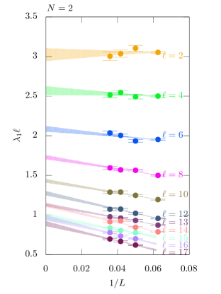
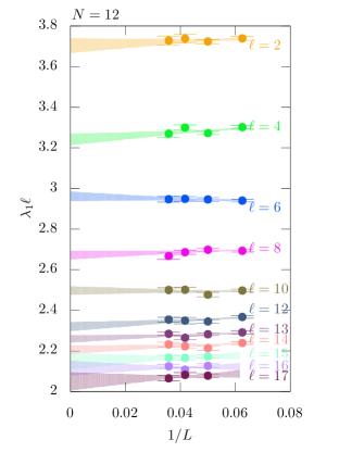
Figure 1: The continuum limits of $\lambda_{1}\ell$ at different fixed $\ell$ using a $1/L$ extrapolation for $N=2$ flavors is shown in the left panel and for $N=12$ in the right panel. The values of $\ell$ are given by the side of the data.

We present the results of our numerical analysis in this section. We have given the list of our simulation points ($\ell$, $L$, $N$) along with the corresponding averages of the first four eigenvalues of the massless Hermitian Wilson-Dirac in Tables-3,4,5,6,7 in Appendix B. Using the eigenvalues at fixed $\ell$ at four different values of $L$, we obtained the continuum eigenvalues, $\lambda_{i}(\ell)$; $i=1,2,3,4$, by using a linear extrapolation in $1/L$. We have also tabulated these continuum values in the same set of tables. To illustrate the extrapolation pictorially, we show these continuum extrapolations along with the 1-$\sigma$ error bands for $\lambda_{1}\ell$ for $N=2$ and $N=12$ in Figure 1.

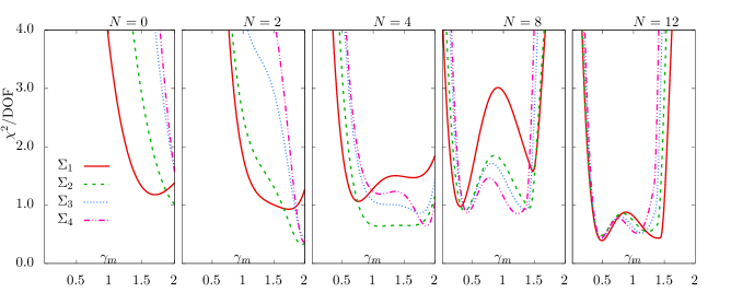
Figure 2: A plot of $\chi^{2}$ per degree of freedom as a function of $\gamma_{m}$ for different flavors $N$. The different curves are obtained from various $\Sigma_{i}$.

Using the continuum extrapolated values of $\lambda_{i}(\ell)$, we obtained $\Sigma_{i}(\ell)$ as defined in Eq. (8). We fit $\Sigma_{i}(\ell)$ as a function of $\ell$ using Eq. (9) with different values of the exponent $\gamma_{m}$. In Figure 2, we show the $\chi^{2}/{\rm DOF}$ for these fits as a function of $\gamma_{m}$ for different $N$, as labelled on top of each panel. The different curves in the panels correspond to $\chi^{2}/{\rm DOF}$ of the fits to the four different $\Sigma_{i}$. In order to easily interpret the plot, a rule of thumb is that the fit using a value of $\gamma_{m}$ is good if its $\chi^{2}/{\rm DOF}$ is about 1, while it being 2 or above is indicative of the fit describing the data poorly. In the different panels, the limit $\gamma_{m}\to 2$ points to a theory with a bilinear condensate and the limit $\gamma_{m}\to 0$ points to a free field behavior.

For the $N=0$ and $N=2$ theories, the $\chi^{2}/{\rm DOF}$ has a minimum around $\gamma_{m}=2$, thereby favoring a non-zero bilinear condensate. The $N=8$ and $N=12$ theories clearly disfavor $\gamma_{m}=2$, instead favoring a scale-invariant behavior with a non-trivial anomalous dimension. For both these $N$, the $\chi^{2}$ minima are seen at two values of $\gamma_{m}$; one at $\gamma_{m}\approx 0.4$ and another at $\gamma_{m}\approx 1.4$. The two allowed values of $\gamma_{m}$ separated by 1, points to the possibility that the $\ell^{-2+0.4}$ behavior of $\Sigma_{i}(\ell)$ describing the data at large values of $\ell$ could either correspond to the leading term in Eq. (9), or it could be the subleading term in Eq. (9) which is dominant in the range of $\ell$ where we have the data, with the leading $\ell^{-2+1.4}$ term becoming dominant only at even larger $\ell$ where we do not have the data. If one assumes a well-behaved $1/\ell$ expansion with successively smaller higher order terms, with no cross-over from one type of leading behavior to another, one would favor the smaller of the allowed values of $\gamma_{m}$, which is around 0.4 to 0.5 for both $N=8$ and 12. At all flavors, the allowed range of $\gamma_{m}$ as deduced from $\Sigma_{1}$ is broader than as allowed by other $\Sigma_{i}$. The most likely cause is that the behavior of the lowest eigenvalue is affected the most by the need to fine tune the Wilson mass to realize massless fermions on the lattice as explained in Appendix A. This is enhanced at $N=4$ as is evident from the flat behavior of the $\chi^{2}$ for $i=1$ at $N=4$. For $N=4$, the range of allowed $\gamma_{m}$ as deduced from the other $i$ are also broad and includes $\gamma_{m}=2$, and hence we are unable to rule out scale-breaking in this case. In the following subsections, we analyze the different $N$ separately.

III.1 $N=0$

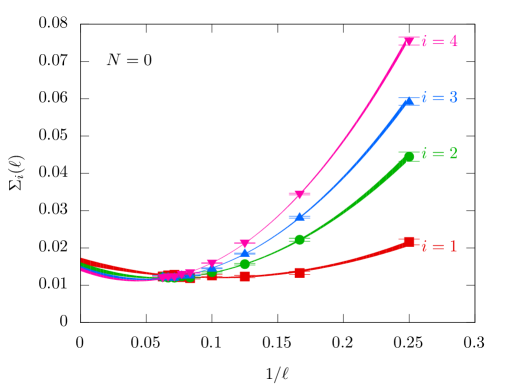
Figure 3: A plot of $\Sigma_{i}(\ell)$ as a function of $\ell$ for $N=0$ flavors i.e., the quenched limit. The different colors correspond to different $i$ as specified in the plot. The data as well as the error-bands of the fit using Eq. (10) are shown. The different $\Sigma_{i}$ extrapolate to about the same value in the infinite volume limit.

Using the four values of $z_{i}$ for $N=0$ in Table 1, we obtained $\Sigma_{i}(\ell)$ from Eq. (8). In Figure 3, we have plotted $\Sigma_{i}(\ell)$ as a function of $1/\ell$. One can see that the asymptotic behavior has set in for $\ell\geq 14$ with a finite value of the bilinear condensate in the $\ell\to\infty$ limit. In the same plot, we have also shown the error bands of fits to the data using Eq. (10). We find the values of $\Sigma_{i}$ extrapolated to infinite $\ell$ for $i=1,2,3,4$ to be $0.0165(8),0.0154(7),0.0147(5)$ and $0.0143(4)$ respectively. It is reassuring that the values of $\Sigma_{i}$ for different $i$ converge to about the same value within errors in the $\ell\to\infty$ limit. By taking the average over all the four values of $\Sigma_{i}(\ell=\infty)$, we quote the value of the bilinear condensate per color degree of freedom for $N=0$ as

$$\frac{\Sigma}{N_{c}}=0.0076\pm 0.0003;\quad N_{c}=2,$$ (12)

with the error being purely statistical. We take the spread of values in the four different $\Sigma_{i}$ to be a measure of the systematic errors in the various extrapolations, and we conservatively estimate this systematic error to be about $0.0011$. In the $N=0$ quenched theory, the fermions are used merely as a probe with no back-reaction on the gauge fields. Since the pure $SU(2)$ theory does have a scale, it is not a surprise to find a bilinear condensate in this case. We remind the reader that the above value of condensate is dimensionless and in units of the coupling $g^{2}_{\rm ph}$. When the above value of condensate per color is measured in units of the ’t Hooft coupling, $N_{c}g^{2}_{\rm ph}$, it is roughly a factor of $2$ smaller than the corresponding value in the ’t Hooft limit in Karthik and Narayanan (2016c). It is also interesting to note that a linear extrapolation in $\frac{1}{N_{c}}$ of the $N_{c}=1$ value in Karthik and Narayanan (2017) and the $N_{c}=2$ value obtained here of the quenched condensates in units of ’t Hooft coupling is consistent with the value in the ’t Hooft limit.

III.2 $N=2$

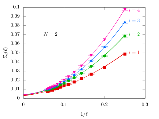
Figure 4: A plot of $\Sigma_{i}(\ell)$ as a function of $\ell$ for $N=2$, with the different symbols and error bands as explained in Figure 3.

We use the four values of $z_{i}$ for $N=2$ in Table 1 to obtain $\Sigma_{i}(\ell)$ from Eq. (8). In Figure 4, we show the $\ell$ dependence of $\Sigma_{i}$. Unlike the $N=0$ theory, we do not see an asymptotic plateauing of the condensate even at the largest $\ell$ we were able to simulate. We have shown the fits of the data to Eq. (10) by the solid lines in the same plot for the different values of $i$. From these extrapolations, we estimate the condensate at infinite volume for $i=1,2,3,4$ to be 0.0030(4), 0.0039(4), 0.0042(4), 0.0042(4) respectively. We find the condensates estimated from different eigenvalues to converge to significantly non-zero values at $\ell=\infty$. As in the case of $N=0$, these extrapolated values of $\Sigma_{i}$ from $i=2,3$ and 4 agree within errors. But, the extrapolated central value of $\Sigma_{1}$ is 30% lower than the others, but still significantly larger than zero. We think this is due to the difficulty in tuning the Wilson mass to obtain exactly massless fermions. One can rectify this in a future study with overlap fermions. Taking the average over the estimates of $\Sigma$ from all the four low-lying eigenvalues, the condensate per color degree of freedom for $N=2$ is

$$\frac{\Sigma}{N_{c}}=0.0019\pm 0.0002;\quad N_{c}=2,$$ (13)

with the error being purely statistical. Taking the spread in the estimated values of $\Sigma_{i}/N_{c}$, a conservative estimate of the systematic error is 0.0006. Note that the value condensate mesured in units of ’t Hooft coupling is lower by a factor of $10$ compared to the one in the ’t Hooft limit.

III.3 $N=4$

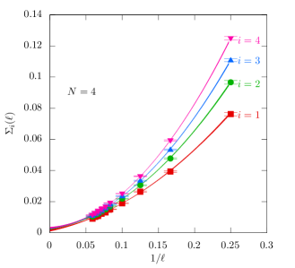
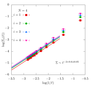
Figure 5: Plots of $\Sigma_{i}(\ell)$ as a function of $\ell$ for $N=4$ in linear scale (left panel) and in log-log scale (right panel). The analysis on the left panel assumes the presence of a non-zero condensate in the infinite volume limit, and hence explicitly sets $\gamma_{m}=2$. The error bands for the infinite volume extrapolations are shown along with the data in the left panel. The analysis on the right panel assumes the absence of a condensate, and hence uses a $\gamma_{m}\neq 2$. A possible $\ell^{-2+\gamma_{m}}$ scaling behavior, with $\gamma_{m}\approx 0.6$, is seen in the large $\ell$ we simulated.

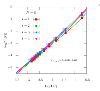
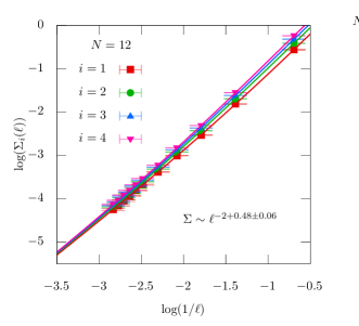
Figure 6: A log-log plot of $\Sigma_{i}(\ell)$ as a function of $\ell$ for $N=8$ and $12$. They clearly show a power-law behavior with the exponent $\gamma_{m}<2$. This suggests $N=8$ and 12 are scale-invariant theories.

For $N=4$, we again use the four corresponding values of $z_{i}$ in Table 1 to obtain $\Sigma_{i}(\ell)$ from Eq. (8). From the third panel of Figure 2 which shows the $\chi^{2}/{\rm DOF}$ as a function of $\gamma_{m}$ for $N=4$, we find a wide range of values of $\gamma_{m}$, including $\gamma_{m}=2$, that fits the data well. Therefore, we analyze the data first assuming the presence of non-vanishing condensate, in which case we force $\gamma_{m}=2$ and extrapolate the condensate to infinite volume using Eq. (10). This procedure is shown on a linear scale on the left panel of Figure 5. This leads to the values 0.0015(6), 0.0026(6), 0.0030(5), 0.0032(5) for $\Sigma_{1},\Sigma_{2},\Sigma_{3}$ and $\Sigma_{4}$ respectively in the infinite volume limit. We stress that this analysis involves a prior assumption that $\gamma_{m}=2$, and with this assumption we find a possible non-zero condensate. However, on the right panel of Figure 5, we again show $\Sigma_{i}(\ell)$ as a function of $1/\ell$, but on a log-log plot; a power-law behavior will be seen as a straight line on this scale with the slope being the scaling exponent. Now we can see a possible scaling behavior setting in for $\ell>13$. Assuming a perfect $\ell^{-2+\gamma_{m}}$ behavior for $\ell>13$, we find $\gamma_{m}\approx 0.60$ if the theory is scale-invariant. Thus, the two different analyses leads to two different conclusions. A more careful analysis, using even larger values of $\ell$ than we have used, could place this theory on either side of the critical value $N^{*}$.

III.4 $N=8$ and $12$

Having found an indication of transition from scale-broken to conformal phase at $N\approx 4$, we studied $N=8$ and 12 to see if we find strong evidence for a scale-invariant behavior. In Figure 6, we show the behavior of $\Sigma_{i}(\ell)$ as a function of $\ell$ in log-log plots. For both $N=8$ and 12 we find an asymptotic power-law behavior setting in for $\ell>4$. Incorporating the $1/\ell$ and $1/\ell^{2}$ corrections in Eq. (9), we find the values for $\gamma_{m}$ to be 0.38(8) and 0.48(6) for $N=8$ and 12 corresponding to the first minima of the two seen in the last two panels of Figure 2. The fits to the data with these exponents are also shown along with the data in Figure 6. Thus $N\geq 8$ clearly lie in the scale-invariant phase. Even though there is strong evidence for the presence of $\gamma_{m}\neq 2$, we nevertheless performed an analysis assuming the presence of non-zero $\Sigma_{i}$ using Eq. (10). We find the extrapolated values of the condensates, after averaging over the four different estimates $\Sigma_{i}$, to be $0(2)\times 10^{-6}$ and $0(7)\times 10^{-6}$ for $N=8$ and 12 respectively, and hence consistent with a scale-invariant behavior.

III.5 Combined analysis of condensate

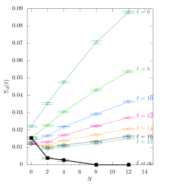
Figure 7: A plot of the condensate $\Sigma_{2}(\ell)$, as determined from the second smallest eigenvalue, shown as a function of fermion flavor $N$ at different fixed $\ell$, as labelled by the side. The open symbols correspond to the value of condensate determined at finite $\ell$, as defined in Eq. (8). The black solid symbol corresponds to the extrapolated value of condensate at infinite $\ell$. The points are connected by lines to aid the eye.

We consolidate our results on the condensate from different flavors in Figure 7. For the sake of clarity, we have only shown the data for the second eigenvalue. The plot shows the condensate at finite $\ell$ as we have defined using Eq. (8). In the same plot, we also show the expected value of condensate at infinite volume, with the starting assumption that there is no non-trivial scaling dimension present, which forces $\gamma_{m}=2$. As we have explained, this is a good assumption for $N=0$ and 2, and we find a non-zero condensate in these cases. While this is a bad assumption for $N=8$ and 12, the extrapolated values of the condensate in these cases is nevertheless consistent with zero. However, our results are inconclusive about the $N=4$ case; analyses assuming $\gamma_{m}=2$ as well as $\gamma_{m}<2$ are consistent with the data. Thus, we have shown a non-zero value of condensate in Figure 7. We could not study any critical $\Sigma(N)\sim|N-N^{*}|^{\Delta}$ behavior near $N^{*}\approx 4$ given the access to only two scale-broken integer number of dynamical flavors.

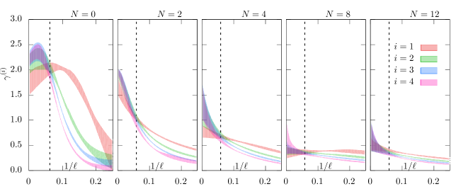
Figure 8: The flow of $\gamma^{(i)}(\ell)$ as defined in Eq. (14) to its asymptotic value $\gamma_{m}$ in the infinite volume limit for $N=0,2,4,8$ and 12. The different colored error bands correspond $i=1,2,3,4$. The dashed vertical lines correspond to the value of $1/\ell$ for the largest $\ell$ we have the data for, at each $N$.

III.6 A flow from UV to IR

As explained in the beginning of this section, we used Eq. (9) to describe the data and also to find the value of $\gamma_{m}$ that best describes the asymptotic finite-size scaling behavior of the low-lying eigenvalues. Once we have fit the data using Eq. (9), we can define an $\ell$ dependent $\gamma_{m}$ as

$$\gamma^{(i)}(\ell)\equiv 2+\frac{\partial\log\left(\Sigma_{i}(\ell)\right)}{\partial\log(\ell)},$$ (14)

which will flow from $\gamma^{(i)}=0$ in the UV limit $\ell\to 0$, to $\gamma^{(i)}=\gamma_{m}$ in the IR limit $\ell\to\infty$ for all $i$. In Figure 8, we show this flow for all $N$. As expected the value of $\gamma^{(i)}(\ell)$ increases from values closer to zero in smaller volumes as $\ell$ is increased. For $N=0$ and $N=2$, in the infinite $\ell$ limit, the values of $\gamma^{(i)}$ converge to values around 2, thereby showing the presence of condensate for these smaller values of $N$. For $N=8$ and 12, $\gamma^{(i)}$ clearly flows to asymptotic values smaller than 1, indicating the presence of non-trivial mass anomalous dimension characteristic of infra-red fixed points in these theories. For $N=4$, $\gamma^{(1)}$ seems to flow to value less than 1, but $\gamma^{(i)}$ from larger $i$ flow to values around 1.5 at $68\%$ confidence. However, at 94% confidence levels, the flow to $\gamma=2$ is also possible. So, this plot sums up our restricted knowledge of the $N=4$ theory. In order to give confidence in the extrapolations to $\ell\to\infty$, in the different panels, we have separated the range of $\ell$ where we have the data from the range of larger $\ell$ where we do not. The flow to infinite $\ell$ which is extrapolative, is smooth and well-behaved. In all the panels, in the range of $\ell$ where we have the data, the values of $\gamma^{(i)}(\ell)$ from different $i$ do not in general agree. But $\gamma^{(i)}$ for $N=0,2,8$ and 12 converge to values consistent with each other in the infinite $\ell$ limit thereby giving confidence in the conclusions drawn in these cases.

IV Conclusions

We have performed a numerical analysis of three dimensional $SU(2)$ gauge theory coupled to an even number of massless fermions in such a way that parity is preserved. We used Wilson fermions instead of overlap fermions to reduce the computational cost. The price to pay was the absence of the full $Sp(N)$ flavor symmetry away from the continuum limit but this did not prevent us from extracting the critical number of fermion flavors.

We studied the finite volume behavior of the low lying Dirac spectrum in a periodic finite physical volume of size $\ell^{3}$ using two different forms, namely, Eq. (9) and Eq. (10). The first one has the anomalous dimension, $\gamma_{m}$, as a parameter that we varied to find the best fit. We found that the data clearly favored $\gamma_{m}=2$ for $N=2$ and $N=4$ and the data clearly favored $\gamma_{m}<2$ for $N=8$ and $N=12$. Given the numerical limitations in obtaining results at arbitrary large values of $\ell$, our data showed it did not favor $\gamma_{m}=2$ for $N=4$. The presence of a non-zero bilinear condensate for $N=0$ and $N=2$, and the absence of one for $N=8$ and $N=12$ remained true when the data was analyzed using Eq. (10) which did not have the freedom of choosing a $\gamma_{m}$ away from integer values. Analysis of the $N=4$ data using Eq. (10) suggests a small value for the bilinear condensate.

We therefore conclude that the critical number of flavors is somewhere between $N=4$ or $N=6$ and we are not able to exclude $N=4$ using the analysis presented in this paper. Having narrowed down the critical value of the number of flavors to one of two integers, the next step is to study the $N=4$ and $N=6$ theories using overlap Karthik and Narayanan (2016b) or domain-wall fermions Hands (2016, 2015). Since the $U(N)$ flavor symmetry as well as the larger $Sp(N)$ global symmetry will be exact in the lattice theory, the behavior of all low lying eigenvalues can be used in the numerical analysis with equal confidence. Furthermore, one can also study the propagator of scalar and vector mesons and extract the behavior of their masses in finite volume.

The analysis presented in this paper clearly shows that one can use $SU(2)$ gauge theories with massless fermions in three dimensions to numerically study the transition from scale invariant behavior to one that generates a scale using continuum finite volume analysis. It will also be interesting to test the predictions for symmetry breaking in Komargodski and Seiberg (2018)

Appendix A Wilson fermions in three dimensions

In our lattice simulation, both the gauge field as well as the $N$ flavors of fermions are dynamical. That is, the Boltzmann weight $e^{-S}$ in our simulation using the Hybrid Monte Carlo (HMC) technique Duane et al. (1987) uses $S=S_{f}+S_{g}$, where $S_{f}$ and $S_{g}$ are the fermion and gauge action respectively. The lattice variables are the SU$(2)$ gauge-links; a gauge link $U_{\mu}(n)$ is an $SU(2)$ matrix that represents the parallel transporter from site $n=(n_{1},n_{2},n_{3})$ to site $(n+\hat{\mu})$, with $1\leq n_{i}\leq L$. We impose periodic boundary condition for both the gauge field as well as the fermions in all three directions of the lattice; for SU$(2)$ theory this boundary condition is sufficient since both $1$ as well as $-1$ are part of the gauge group. We use the standard single plaquette gauge action, namely,

$$S_{g}=-\frac{2L}{\ell}\sum_{n}\sum^{3}_{\mu>\nu=1}{\rm Tr}\ P_{\mu\nu}(n),$$ (15)

where $P_{\mu\nu}(n)$ is the parallel transporter around a plaquette in $\mu\nu$-plane at lattice site $n$:

$$P_{\mu\nu}=U_{\mu}(n)U_{\nu}(n+\hat{\mu})U^{\dagger}_{\mu}(n+\hat{\nu})U^{\dagger}_{\nu}(n).$$ (16)

We reduced lattice spacing effect in fermion action as well as fermionic observables by smoothening the gauge field that enters the Dirac operator using the technique of gauge-link smearing. For this, we used 1-level improved stout links Morningstar and Peardon (2004), denoted by $V_{\mu}(n)$:

$$V_{\mu}(n)=e^{i\frac{s}{4}Q_{\mu}(n)}U_{\mu}(n)\quad{\rm where}\quad Q_{\mu}(n)=\sum_{\nu\neq\mu}\frac{1}{2i}\left(P_{\mu\nu}(n)-\frac{1}{2}{\rm Tr}P_{\mu\nu}(n)\right)-{\rm h.c}.$$ (17)

We used an optimum value $s=0.65$ where the value of the smeared plaquette was maximized. For the regularized two-component Dirac operator in Eq. (4), we used the two-component Wilson-Dirac operator $C_{W}$ given by

$$C_{W}(n,m)=(-3+M_{P})\delta_{n,m}+\frac{1}{2}\sum_{\mu=1}^{3}\left\{\left(1+\sigma_{\mu}\right)V_{\mu}(n)\delta_{n+\hat{\mu},m}+\left(1-\sigma_{\mu}\right)V^{\dagger}_{\mu}(n-\hat{\mu})\delta_{n-\hat{\mu},m}\right\},$$ (18)

where $\sigma_{\mu}$ are the Pauli matrices, and $M_{P}$ is the Wilson mass which needs to be fine-tuned to non-zero values at finite lattice spacings in order study massless continuum fermions. The above two-component Wilson-Dirac operator satisfies $C^{t}_{W}(n,m)=\sigma_{2}\tau_{2}C_{W}(n,m)\sigma_{2}\tau_{2}$, and hence there is a $Sp(1)$ symmetry associated with a single flavor of two-component Wilson fermion even at finite lattice spacing. We incorporated the resulting fermion determinant, $\det\left(C_{W}C^{\dagger}_{W}\right)^{N/2}$, from the $N/2$ parity-invariant pairs of two-component Wilson-Dirac fermions in our HMC simulation using using $N/2$ pseudo-fermion random vectors as explained in Karthik and Narayanan (2016a). In the HMC, we were able to marginally optimize the molecular dynamics stepsize by using the Omelyan symplectic integrator Omelyan et al. (2002) as well as by tuning the stepsize at run-time such that the acceptance is above 80%.

$N$	$L$	$M_{1}\times 10^{2}$	$M_{2}\times 10^{3}$	$M_{3}\times 10^{4}$
0	16	2.45	2.70	7.58
	20	2.14	1.48	5.52
	24	1.26	2.58	3.34
	28	0.82	2.82	2.25
	32	0.41	3.18	1.39
2	16	3.09	3.66	4.80
	20	1.82	3.62	3.14
	24	1.25	3.60	1.89
	28	0.69	3.79	1.11
4	16	2.98	5.43	2.61
	20	1.98	4.11	3.04
	24	1.21	4.19	1.14
	28	0.96	3.62	0.84
8	16	3.33	5.92	1.08
	20	2.08	4.90	0.82
	24	1.41	4.21	0.60
	28	0.98	3.79	0.37
12	16	3.91	4.78	1.18
	20	2.36	4.41	0.66
	24	1.72	3.72	0.49
	28	1.12	3.57	0.27

Table 2: Table of values for $M_{1},M_{2}$ and $M_{3}$ which parametrize the $\ell$ dependence of the tuned Wilson mass $M_{P}$ as given in Eq. (19). The values at different $L$ and $N$ are tabulated.

As discussed earlier, the eigenvalues of the four-component Hermitian Wilson-Dirac operator, $D_{W}$, appear in $\pm$ pairs. The operator $C_{W}$ is not anti-Hermitian but becomes essentially one upon tuning $M_{P}$ to achieve massless fermions. As such, the $Sp(1)\times Sp(1)$ symmetry at finite lattice spacing becomes the full $Sp(2)$ symmetry only in the continuum limit. But, the positive eigenvalues of $D_{W}$ can be used to study the presence or absence of a bilinear condensate as discussed in the context of $U(N)$ flavor symmetry Karthik and Narayanan (2016a). In order to realize massless fermions, we tuned the value of $M_{P}$ at each simulation point to that value where the lowest eigenvalue of $C_{W}C^{\dagger}_{W}$ is minimized when measured over a small ensemble of thermalized configurations at that simulation point. Since these tuned $M_{P}$ are required for any future computation at larger $\ell$ and $L$, and also for normalizing the eigenvalues of the overlap operator which makes use of the Wilson-Dirac kernel Karthik and Narayanan (2016b), we parametrize the tuned value of $M_{P}(\ell)$ for different $L$ and $N$ using

$$M_{P}(\ell)=M_{1}+M_{2}\ell+M_{3}\ell^{2},$$ (19)

and tabulate these parameters in Table 2.

We used Ritz algorithm Kalkreuter and Simma (1996) to compute the four low-lying eigenvalues of $\sqrt{C^{\dagger}_{W}C_{W}}$. We measured the eigenvalues every five trajectories of HMC after thermalization, and this way we collected about 3500 to 4500 measurements at different $\ell$, $L$ and $N$. We accounted for autocorrelations in the data by using blocked jack-knife error analysis. The simulation points at $N=0,2,4,8$ and 12 along with the low-lying eigenvalue measurements are tabulated in Appendix B.

Appendix B Tables of measurements

In the following tables, we have given the values and the errors of the four low-lying eigenvalues of the Dirac operator for $N=0,2,4,8$ and 16. For each physical $\ell$, we have given these measurements made using different $L^{3}$ lattices. The $L=\infty$ values are the continuum values obtained through a linear $1/L$ extrapolation.

$\ell$	$L$	$\lambda_{1}\ell$	$\lambda_{2}\ell$	$\lambda_{3}\ell$	$\lambda_{4}\ell$
4	16	1.942(29)	2.295(27)	2.748(20)	3.004(18)
	20	1.892(43)	2.246(42)	2.711(28)	2.965(27)
	24	1.902(46)	2.249(44)	2.723(33)	2.971(31)
	28	1.917(37)	2.261(34)	2.722(26)	2.973(24)
	32	1.891(56)	2.246(53)	2.704(41)	2.959(37)
	$\infty$	1.857(66)	2.199(61)	2.674(46)	2.919(42)
6	16	1.227(18)	1.902(16)	2.454(11)	2.816(9)
	20	1.267(18)	1.928(16)	2.473(10)	2.830(8)
	24	1.291(24)	1.938(19)	2.485(11)	2.834(8)
	28	1.230(28)	1.881(22)	2.447(12)	2.800(11)
	32	1.314(38)	1.973(30)	2.506(19)	2.854(15)
	$\infty$	1.343(43)	1.958(35)	2.497(22)	2.842(19)
8	16	0.693(9)	1.419(9)	2.003(6)	2.440(5)
	20	0.727(10)	1.473(7)	2.044(7)	2.480(6)
	24	0.736(15)	1.467(18)	2.059(12)	2.492(9)
	28	0.759(12)	1.485(12)	2.065(11)	2.505(8)
	32	0.727(17)	1.473(16)	2.065(10)	2.509(6)
	$\infty$	0.814(20)	1.562(20)	2.144(15)	2.585(10)
10	16	0.450(5)	0.997(8)	1.508(7)	1.949(6)
	20	0.457(6)	1.044(9)	1.567(8)	2.009(8)
	24	0.476(7)	1.065(8)	1.602(7)	2.047(6)
	28	0.467(8)	1.061(12)	1.611(9)	2.058(8)
	32	0.480(8)	1.066(14)	1.604(13)	2.069(10)
	$\infty$	0.508(12)	1.160(17)	1.745(15)	2.210(12)
12	16	0.320(3)	0.705(5)	1.097(5)	1.465(6)
	20	0.327(3)	0.748(6)	1.163(6)	1.550(6)
	24	0.340(4)	0.777(6)	1.211(7)	1.605(6)
	28	0.339(5)	0.776(8)	1.209(9)	1.604(9)
	32	0.350(5)	0.805(8)	1.237(9)	1.646(8)
	$\infty$	0.375(7)	0.899(11)	1.389(12)	1.832(13)

$\ell$	$L$	$\lambda_{1}\ell$	$\lambda_{2}\ell$	$\lambda_{3}\ell$	$\lambda_{4}\ell$
13	16	0.279(2)	0.600(4)	0.937(5)	1.260(6)
	20	0.285(3)	0.634(6)	1.000(9)	1.347(10)
	24	0.293(3)	0.658(7)	1.031(7)	1.386(7)
	28	0.291(4)	0.658(6)	1.036(7)	1.404(8)
	32	0.294(5)	0.673(7)	1.062(11)	1.432(14)
	$\infty$	0.312(6)	0.748(9)	1.187(12)	1.613(13)
14	16	0.251(3)	0.521(3)	0.802(4)	1.082(5)
	20	0.258(3)	0.553(4)	0.854(5)	1.155(5)
	24	0.257(4)	0.578(6)	0.902(7)	1.224(8)
	28	0.250(3)	0.577(5)	0.911(7)	1.237(7)
	32	0.253(5)	0.593(11)	0.938(12)	1.270(12)
	$\infty$	0.256(6)	0.665(9)	1.069(11)	1.460(12)
15	20	0.226(3)	0.482(4)	0.750(5)	1.016(6)
	24	0.226(3)	0.497(4)	0.779(5)	1.052(6)
	28	0.228(4)	0.513(6)	0.804(7)	1.095(8)
	32	0.225(3)	0.516(6)	0.813(9)	1.110(11)
	$\infty$	0.226(8)	0.578(13)	0.927(18)	1.274(21)
16	20	0.228(2)	0.453(3)	0.675(4)	0.900(4)
	24	0.203(3)	0.441(4)	0.687(4)	0.931(4)
	28	0.199(2)	0.440(3)	0.700(5)	0.958(5)
	32	0.204(3)	0.462(5)	0.721(8)	0.988(10)
	$\infty$	0.203(12)	0.500(19)	0.808(27)	1.139(29)

Table 3: Measurements for $N=0$.

$\ell$	$L$	$\lambda_{1}\ell$	$\lambda_{2}\ell$	$\lambda_{3}\ell$	$\lambda_{4}\ell$
2	16	3.053(15)	3.216(15)	3.435(14)	3.568(14)
	20	3.105(37)	3.269(36)	3.483(32)	3.616(31)
	24	3.037(46)	3.204(45)	3.429(39)	3.564(38)
	28	3.005(52)	3.165(51)	3.402(44)	3.535(43)
	$\infty$	3.026(80)	3.191(79)	3.429(70)	3.564(68)
3	16	2.771(10)	3.001(10)	3.266(9)	3.439(9)
	20	2.701(36)	2.934(36)	3.216(30)	3.388(30)
	24	2.799(42)	3.022(42)	3.286(35)	3.460(33)
	28	2.783(45)	3.004(45)	3.274(38)	3.446(36)
	$\infty$	2.761(70)	2.975(71)	3.259(59)	3.434(56)
4	16	2.501(14)	2.796(14)	3.112(11)	3.322(10)
	20	2.494(29)	2.790(30)	3.113(25)	3.319(23)
	24	2.546(28)	2.839(28)	3.151(24)	3.357(21)
	28	2.516(34)	2.818(33)	3.121(26)	3.330(25)
	$\infty$	2.570(56)	2.870(55)	3.167(44)	3.372(41)
5	16	2.209(10)	2.589(9)	2.945(8)	3.191(7)
	20	2.252(20)	2.610(19)	2.954(15)	3.204(13)
	24	2.248(26)	2.620(24)	2.968(17)	3.214(18)
	28	2.278(30)	2.645(31)	2.979(25)	3.224(22)
	$\infty$	2.364(46)	2.700(45)	3.014(36)	3.263(32)
6	16	1.953(8)	2.393(7)	2.776(6)	3.061(5)
	20	1.935(17)	2.377(18)	2.771(14)	3.048(12)
	24	2.005(17)	2.426(16)	2.798(11)	3.073(9)
	28	2.036(25)	2.439(24)	2.815(20)	3.086(17)
	$\infty$	2.089(36)	2.475(34)	2.841(26)	3.094(21)
7	16	1.710(9)	2.193(8)	2.595(5)	2.904(5)
	20	1.730(15)	2.200(14)	2.609(12)	2.910(8)
	24	1.773(16)	2.242(17)	2.639(13)	2.942(11)
	28	1.786(27)	2.259(23)	2.642(18)	2.939(16)
	$\infty$	1.881(36)	2.324(34)	2.708(26)	2.989(22)
8	16	1.500(7)	1.998(6)	2.410(5)	2.738(5)
	20	1.564(11)	2.041(10)	2.448(9)	2.762(7)
	24	1.570(12)	2.051(12)	2.457(11)	2.779(8)
	28	1.595(20)	2.061(19)	2.466(14)	2.781(12)
	$\infty$	1.730(26)	2.164(25)	2.555(22)	2.852(18)
9	16	1.337(7)	1.835(6)	2.240(4)	2.578(4)
	20	1.391(11)	1.856(13)	2.270(9)	2.610(7)
	24	1.419(19)	1.872(17)	2.278(15)	2.607(13)
	28	1.463(19)	1.914(19)	2.318(15)	2.635(11)
	$\infty$	1.612(30)	1.981(29)	2.396(23)	2.707(19)

$\ell$	$L$	$\lambda_{1}\ell$	$\lambda_{2}\ell$	$\lambda_{3}\ell$	$\lambda_{4}\ell$
10	16	1.195(6)	1.655(6)	2.060(6)	2.400(5)
	20	1.248(10)	1.708(12)	2.101(9)	2.435(8)
	24	1.289(17)	1.754(15)	2.139(12)	2.473(10)
	28	1.288(13)	1.723(17)	2.131(15)	2.463(11)
	$\infty$	1.433(23)	1.880(27)	2.258(23)	2.574(18)
11	16	1.074(7)	1.502(7)	1.891(6)	2.220(7)
	20	1.132(11)	1.554(10)	1.940(8)	2.272(8)
	24	1.162(14)	1.580(13)	1.962(10)	2.289(9)
	28	1.178(13)	1.591(15)	1.969(12)	2.301(13)
	$\infty$	1.328(24)	1.727(25)	2.092(20)	2.425(21)
12	16	0.958(7)	1.357(6)	1.727(6)	2.056(6)
	20	1.022(11)	1.424(13)	1.789(11)	2.110(11)
	24	1.074(12)	1.469(11)	1.835(10)	2.155(10)
	28	1.073(21)	1.445(22)	1.830(19)	2.138(15)
	$\infty$	1.277(27)	1.656(27)	2.025(23)	2.310(22)
13	16	0.872(7)	1.237(6)	1.582(5)	1.891(4)
	20	0.932(11)	1.301(12)	1.657(10)	1.967(8)
	24	0.961(9)	1.334(11)	1.693(12)	1.996(10)
	28	0.977(14)	1.349(15)	1.708(15)	2.023(14)
	$\infty$	1.133(22)	1.517(23)	1.905(23)	2.216(20)
14	16	0.788(7)	1.129(7)	1.451(6)	1.743(5)
	20	0.846(9)	1.186(7)	1.517(9)	1.816(9)
	24	0.926(11)	1.255(12)	1.575(12)	1.876(11)
	28	0.916(11)	1.248(11)	1.575(11)	1.879(11)
	$\infty$	1.123(21)	1.434(20)	1.768(21)	2.092(19)
15	20	0.777(11)	1.095(13)	1.408(12)	1.698(10)
	24	0.805(10)	1.115(11)	1.428(11)	1.711(10)
	28	0.835(12)	1.161(11)	1.473(9)	1.768(7)
	$\infty$	0.979(45)	1.320(48)	1.636(42)	1.945(34)
16	20	0.700(7)	1.007(10)	1.299(10)	1.566(9)
	24	0.734(11)	1.031(13)	1.323(13)	1.598(13)
	28	0.779(10)	1.075(12)	1.372(10)	1.645(8)
	$\infty$	0.967(34)	1.237(44)	1.546(40)	1.842(33)
17	20	0.621(7)	0.899(9)	1.173(10)	1.426(9)
	24	0.667(7)	0.948(8)	1.222(8)	1.477(8)
	28	0.698(10)	0.980(11)	1.262(10)	1.526(9)
	$\infty$	0.892(33)	1.186(38)	1.484(38)	1.773(36)

Table 4: Measurements for $N=2$.

$\ell$	$L$	$\lambda_{1}\ell$	$\lambda_{2}\ell$	$\lambda_{3}\ell$	$\lambda_{4}\ell$
2	16	3.351(16)	3.509(16)	3.693(14)	3.814(14)
	20	3.309(23)	3.464(22)	3.657(20)	3.778(19)
	24	3.286(31)	3.445(31)	3.638(27)	3.761(26)
	28	3.260(44)	3.421(43)	3.609(39)	3.736(38)
	$\infty$	3.146(63)	3.305(61)	3.514(56)	3.642(54)
4	16	2.778(12)	3.045(11)	3.313(9)	3.503(9)
	20	2.768(19)	3.037(18)	3.302(17)	3.492(15)
	24	2.741(18)	3.010(17)	3.283(14)	3.475(13)
	28	2.776(24)	3.046(25)	3.317(19)	3.500(19)
	$\infty$	2.722(39)	2.990(38)	3.270(31)	3.455(30)
6	16	2.286(10)	2.655(8)	2.970(7)	3.215(6)
	20	2.293(13)	2.666(13)	2.983(11)	3.224(9)
	24	2.285(12)	2.654(11)	2.974(10)	3.213(7)
	28	2.342(18)	2.693(17)	3.009(14)	3.241(14)
	$\infty$	2.343(29)	2.692(26)	3.019(22)	3.234(19)
8	16	1.880(8)	2.303(7)	2.655(6)	2.934(4)
	20	1.899(12)	2.325(10)	2.671(8)	2.952(6)
	24	1.903(12)	2.313(10)	2.660(9)	2.935(8)
	28	1.923(19)	2.344(18)	2.693(14)	2.957(12)
	$\infty$	1.964(28)	2.365(25)	2.706(20)	2.972(16)
10	16	1.568(7)	2.006(6)	2.359(5)	2.651(5)
	20	1.616(9)	2.032(8)	2.387(6)	2.680(5)
	24	1.613(9)	2.037(7)	2.391(7)	2.680(5)
	28	1.668(15)	2.063(18)	2.413(13)	2.688(11)
	$\infty$	1.747(22)	2.111(20)	2.470(17)	2.744(15)
12	16	1.362(8)	1.770(8)	2.115(6)	2.404(5)
	20	1.407(12)	1.805(14)	2.145(9)	2.426(11)
	24	1.416(9)	1.808(8)	2.143(8)	2.428(7)
	28	1.433(11)	1.815(10)	2.157(10)	2.449(9)
	$\infty$	1.527(21)	1.879(20)	2.210(17)	2.494(16)

$\ell$	$L$	$\lambda_{1}\ell$	$\lambda_{2}\ell$	$\lambda_{3}\ell$	$\lambda_{4}\ell$
13	16	1.272(5)	1.661(5)	1.992(5)	2.274(5)
	20	1.322(7)	1.691(6)	2.017(6)	2.306(4)
	24	1.346(12)	1.713(11)	2.049(9)	2.327(7)
	28	1.368(15)	1.730(13)	2.063(11)	2.341(10)
	$\infty$	1.502(22)	1.818(20)	2.152(17)	2.432(16)
14	16	1.204(9)	1.581(8)	1.893(6)	2.168(5)
	20	1.220(10)	1.588(9)	1.914(8)	2.193(7)
	24	1.272(10)	1.623(8)	1.940(8)	2.216(8)
	28	1.267(12)	1.629(10)	1.952(9)	2.226(8)
	$\infty$	1.372(22)	1.697(20)	2.030(17)	2.306(15)
15	20	1.175(7)	1.526(6)	1.835(5)	2.109(6)
	24	1.196(12)	1.547(12)	1.863(10)	2.130(10)
	28	1.239(15)	1.573(13)	1.876(13)	2.141(11)
	$\infty$	1.369(45)	1.683(41)	1.987(36)	2.226(35)
16	20	1.103(7)	1.442(7)	1.736(6)	1.998(5)
	24	1.140(9)	1.473(9)	1.769(8)	2.035(8)
	28	1.144(14)	1.472(13)	1.772(12)	2.036(11)
	$\infty$	1.278(40)	1.578(38)	1.888(34)	2.162(31)
17	20	1.052(7)	1.382(8)	1.667(8)	1.919(8)
	24	1.064(10)	1.376(9)	1.676(9)	1.931(9)
	28	1.123(9)	1.436(10)	1.721(10)	1.973(11)
	$\infty$	1.276(34)	1.533(35)	1.831(36)	2.085(35)

Table 5: Measurements for $N=4$.

$\ell$	$L$	$\lambda_{1}\ell$	$\lambda_{2}\ell$	$\lambda_{3}\ell$	$\lambda_{4}\ell$
2	16	3.597(18)	3.746(18)	3.903(16)	4.016(16)
	20	3.582(17)	3.732(16)	3.895(15)	4.006(15)
	24	3.602(24)	3.749(24)	3.912(22)	4.025(22)
	28	3.596(30)	3.740(30)	3.903(27)	4.018(26)
	$\infty$	3.593(52)	3.735(52)	3.909(47)	4.023(46)
4	16	3.084(13)	3.323(13)	3.541(11)	3.706(10)
	20	3.098(13)	3.330(13)	3.545(10)	3.710(10)
	24	3.092(18)	3.332(16)	3.549(15)	3.715(13)
	28	3.084(18)	3.317(18)	3.537(16)	3.705(14)
	$\infty$	3.097(35)	3.326(34)	3.545(30)	3.715(27)
6	16	2.711(9)	3.002(8)	3.257(7)	3.456(6)
	20	2.679(15)	2.984(14)	3.242(11)	3.442(11)
	24	2.695(16)	2.988(16)	3.241(14)	3.441(13)
	28	2.666(25)	2.958(24)	3.225(21)	3.427(19)
	$\infty$	2.626(35)	2.930(33)	3.194(29)	3.398(27)
8	16	2.379(10)	2.711(10)	2.986(9)	3.207(7)
	20	2.382(10)	2.715(8)	2.992(8)	3.215(6)
	24	2.374(13)	2.708(12)	2.989(9)	3.213(8)
	28	2.375(15)	2.708(14)	2.983(10)	3.206(10)
	$\infty$	2.370(27)	2.705(27)	2.985(21)	3.215(19)
10	16	2.147(10)	2.497(8)	2.780(7)	3.014(7)
	20	2.158(11)	2.507(10)	2.788(8)	3.021(7)
	24	2.149(14)	2.504(13)	2.786(10)	3.018(9)
	28	2.193(18)	2.528(18)	2.809(14)	3.038(13)
	$\infty$	2.208(30)	2.544(28)	2.823(23)	3.047(20)
12	16	1.957(10)	2.301(8)	2.589(7)	2.821(6)
	20	1.962(12)	2.318(12)	2.596(10)	2.834(8)
	24	1.946(14)	2.289(13)	2.584(11)	2.825(9)
	28	1.972(19)	2.316(18)	2.592(15)	2.833(13)
	$\infty$	1.963(30)	2.312(27)	2.590(23)	2.845(20)

$\ell$	$L$	$\lambda_{1}\ell$	$\lambda_{2}\ell$	$\lambda_{3}\ell$	$\lambda_{4}\ell$
13	16	1.878(11)	2.222(9)	2.504(7)	2.737(6)
	20	1.885(7)	2.239(6)	2.520(6)	2.754(5)
	24	1.883(18)	2.237(17)	2.516(13)	2.757(10)
	28	1.909(16)	2.250(14)	2.533(12)	2.770(9)
	$\infty$	1.930(31)	2.287(26)	2.566(22)	2.811(17)
14	16	1.813(8)	2.161(7)	2.430(6)	2.665(5)
	20	1.819(11)	2.152(11)	2.429(8)	2.666(8)
	24	1.839(11)	2.174(11)	2.452(8)	2.686(8)
	28	1.858(15)	2.182(14)	2.455(11)	2.688(10)
	$\infty$	1.899(24)	2.196(23)	2.487(19)	2.719(16)
15	20	1.748(11)	2.082(10)	2.360(8)	2.591(8)
	24	1.758(12)	2.081(11)	2.365(9)	2.602(8)
	28	1.790(16)	2.127(14)	2.393(11)	2.629(10)
	$\infty$	1.873(52)	2.201(46)	2.459(38)	2.711(35)
16	20	1.677(13)	2.015(10)	2.290(10)	2.522(9)
	24	1.715(11)	2.044(11)	2.316(8)	2.546(8)
	28	1.729(13)	2.054(12)	2.325(13)	2.557(10)
	$\infty$	1.868(50)	2.161(44)	2.424(43)	2.651(37)
17	20	1.621(12)	1.953(12)	2.230(9)	2.461(8)
	24	1.663(7)	1.980(6)	2.249(6)	2.479(5)
	28	1.668(14)	1.992(12)	2.267(12)	2.489(10)
	$\infty$	1.814(49)	2.098(46)	2.357(40)	2.564(33)

Table 6: Measurements for $N=8$.

$\ell$	$L$	$\lambda_{1}\ell$	$\lambda_{2}\ell$	$\lambda_{3}\ell$	$\lambda_{4}\ell$
2	16	3.739(9)	3.879(9)	4.027(9)	4.133(8)
	20	3.724(11)	3.868(11)	4.016(10)	4.125(9)
	24	3.738(23)	3.877(23)	4.025(22)	4.133(21)
	28	3.728(23)	3.874(24)	4.021(21)	4.127(21)
	$\infty$	3.705(36)	3.856(37)	4.003(34)	4.114(32)
4	16	3.302(9)	3.510(9)	3.702(8)	3.852(7)
	20	3.273(8)	3.489(8)	3.681(7)	3.834(8)
	24	3.300(13)	3.514(12)	3.710(12)	3.857(11)
	28	3.270(18)	3.483(17)	3.676(15)	3.828(14)
	$\infty$	3.243(27)	3.473(27)	3.667(24)	3.820(22)
6	16	2.940(6)	3.198(6)	3.422(6)	3.599(5)
	20	2.946(9)	3.201(8)	3.423(6)	3.599(6)
	24	2.949(11)	3.209(11)	3.431(9)	3.605(9)
	28	2.947(14)	3.211(12)	3.437(11)	3.616(10)
	$\infty$	2.963(22)	3.227(21)	3.450(18)	3.626(16)
8	16	2.693(6)	2.973(6)	3.211(6)	3.403(5)
	20	2.698(6)	2.982(6)	3.219(5)	3.407(4)
	24	2.686(10)	2.975(9)	3.219(7)	3.413(7)
	28	2.668(17)	2.946(16)	3.189(12)	3.387(11)
	$\infty$	2.673(22)	2.967(21)	3.210(18)	3.407(16)
10	16	2.497(7)	2.793(6)	3.038(6)	3.238(5)
	20	2.477(11)	2.775(10)	3.021(10)	3.225(9)
	24	2.501(12)	2.805(11)	3.049(8)	3.249(7)
	28	2.500(11)	2.799(10)	3.044(8)	3.245(8)
	$\infty$	2.498(21)	2.807(18)	3.054(15)	3.257(15)
12	16	2.367(6)	2.671(6)	2.912(5)	3.111(5)
	20	2.345(10)	2.646(9)	2.893(8)	3.097(6)
	24	2.349(15)	2.651(13)	2.897(10)	3.098(9)
	28	2.354(12)	2.653(12)	2.903(9)	3.103(8)
	$\infty$	2.321(22)	2.613(21)	2.877(17)	3.082(15)

$\ell$	$L$	$\lambda_{1}\ell$	$\lambda_{2}\ell$	$\lambda_{3}\ell$	$\lambda_{4}\ell$
13	16	2.291(8)	2.588(7)	2.829(6)	3.029(6)
	20	2.282(6)	2.590(5)	2.833(4)	3.034(3)
	24	2.265(10)	2.577(9)	2.820(7)	3.028(7)
	28	2.284(8)	2.581(8)	2.825(8)	3.030(7)
	$\infty$	2.260(19)	2.568(17)	2.816(15)	3.032(14)
14	16	2.239(6)	2.532(6)	2.777(6)	2.981(4)
	20	2.214(12)	2.520(11)	2.766(9)	2.973(7)
	24	2.223(12)	2.521(11)	2.770(9)	2.975(7)
	28	2.232(11)	2.532(11)	2.775(8)	2.980(7)
	$\infty$	2.207(21)	2.518(20)	2.765(16)	2.972(14)
15	20	2.173(9)	2.472(9)	2.722(7)	2.923(6)
	24	2.166(10)	2.469(9)	2.711(7)	2.911(5)
	28	2.167(12)	2.469(14)	2.714(11)	2.917(9)
	$\infty$	2.150(41)	2.461(42)	2.684(34)	2.886(28)
16	20	2.126(10)	2.425(8)	2.666(8)	2.868(6)
	24	2.108(11)	2.407(9)	2.654(8)	2.856(7)
	28	2.124(9)	2.422(8)	2.668(9)	2.869(7)
	$\infty$	2.115(37)	2.407(32)	2.663(32)	2.862(27)
17	20	2.078(10)	2.375(9)	2.613(7)	2.818(6)
	24	2.082(11)	2.369(10)	2.610(7)	2.814(7)
	28	2.065(13)	2.358(13)	2.600(10)	2.805(9)
	$\infty$	2.050(44)	2.324(41)	2.576(32)	2.780(29)

Table 7: Measurements for $N=12$.

References

- Magnea (2000) U. Magnea, Phys. Rev. D61, 056005 (2000), eprint hep-th/9907096.
- Neuberger (1998) H. Neuberger, Phys. Lett. B434, 99 (1998), eprint hep-lat/9803011.
- Pisarski (1984) R. D. Pisarski, Phys.Rev. D29, 2423 (1984).
- Vafa and Witten (1984) C. Vafa and E. Witten, Commun.Math.Phys. 95, 257 (1984).
- Karthik and Narayanan (2016a) N. Karthik and R. Narayanan, Phys. Rev. D93, 045020 (2016a), eprint 1512.02993.
- Karthik and Narayanan (2016b) N. Karthik and R. Narayanan, Phys. Rev. D94, 065026 (2016b), eprint 1606.04109.
- Wang et al. (2017) C. Wang, A. Nahum, M. A. Metlitski, C. Xu, and T. Senthil (2017), eprint 1703.02426.
- Qin et al. (2017) Y. Q. Qin, Y.-Y. He, Y.-Z. You, Z.-Y. Lu, A. Sen, A. W. Sandvik, C. Xu, and Z. Y. Meng, Phys. Rev. X7, 031052 (2017), eprint 1705.10670.
- Karthik and Narayanan (2017) N. Karthik and R. Narayanan (2017), eprint 1705.11143.
- Wen (2004) X. G. Wen, Quantum field theory of many-body systems: From the origin of sound to an origin of light and electrons (2004).
- Lee et al. (2006) P. A. Lee, N. Nagaosa, and X.-G. Wen, Rev. Mod. Phys. 78, 17 (2006).
- Xu (2008) C. Xu, Phys. Rev. B 78, 054432 (2008), URL https://link.aps.org/doi/10.1103/PhysRevB.78.054432.
- Karthik and Narayanan (2016c) N. Karthik and R. Narayanan, Phys. Rev. D94, 045020 (2016c), eprint 1607.03905.
- Dagotto et al. (1991) E. Dagotto, A. Kocifá, and J. Kogut, Nuclear Physics B 362, 498 (1991), ISSN 0550-3213, URL http://www.sciencedirect.com/science/article/pii/055032139190571E.
- Peskin and Schroeder (1995) M. E. Peskin and D. V. Schroeder, An Introduction to quantum field theory (Addison-Wesley, Reading, USA, 1995), ISBN 9780201503975, 0201503972, URL http://www.slac.stanford.edu/~mpeskin/QFT.html.
- Goldman and Mulligan (2016) H. Goldman and M. Mulligan, Phys. Rev. D94, 065031 (2016), eprint 1606.07067.
- Appelquist and Nash (1990) T. Appelquist and D. Nash, Phys. Rev. Lett. 64, 721 (1990).
- Appelquist et al. (1988) T. Appelquist, D. Nash, and L. C. R. Wijewardhana, Phys. Rev. Lett. 60, 2575 (1988).
- Hands (2016) S. Hands, Phys. Lett. B754, 264 (2016), eprint 1512.05885.
- Hands (2015) S. Hands, JHEP 09, 047 (2015), eprint 1507.07717.
- Damgaard et al. (1998) P. H. Damgaard, U. M. Heller, A. Krasnitz, and T. Madsen, Phys. Lett. B440, 129 (1998), eprint hep-lat/9803012.
- Bursa and Teper (2006) F. Bursa and M. Teper, Phys. Rev. D74, 125010 (2006), eprint hep-th/0511081.
- Narayanan et al. (2007) R. Narayanan, H. Neuberger, and F. Reynoso, Phys. Lett. B651, 246 (2007), eprint 0704.2591.
- Del Debbio and Zwicky (2010) L. Del Debbio and R. Zwicky, Phys. Rev. D82, 014502 (2010), eprint 1005.2371.
- Verbaarschot and Zahed (1994) J. J. M. Verbaarschot and I. Zahed, Phys. Rev. Lett. 73, 2288 (1994), eprint hep-th/9405005.
- Nagao and Nishigaki (2001) T. Nagao and S. M. Nishigaki, Phys. Rev. D63, 045011 (2001), eprint hep-th/0005077.
- Komargodski and Seiberg (2018) Z. Komargodski and N. Seiberg, JHEP 01, 109 (2018), eprint 1706.08755.
- Duane et al. (1987) S. Duane, A. Kennedy, B. Pendleton, and D. Roweth, Phys.Lett. B195, 216 (1987).
- Morningstar and Peardon (2004) C. Morningstar and M. J. Peardon, Phys. Rev. D69, 054501 (2004), eprint hep-lat/0311018.
- Omelyan et al. (2002) I. P. Omelyan, I. M. Mryglod, and R. Folk, Phys. Rev. E 65, 056706 (2002), URL https://link.aps.org/doi/10.1103/PhysRevE.65.056706.
- Kalkreuter and Simma (1996) T. Kalkreuter and H. Simma, Comput. Phys. Commun. 93, 33 (1996), eprint hep-lat/9507023.