Spin Conductance and Spin Conductivity
in Topological Insulators:
Analysis of Kubo-like terms

Abstract.

We investigate spin transport in $2$-dimensional insulators, with the long-term goal of establishing whether any of the transport coefficients corresponds to the Fu-Kane-Mele index which characterizes $2d$ time-reversal-symmetric topological insulators.

Inspired by the Kubo theory of charge transport, and by using a proper definition of the spin current operator [SZXN], we define the Kubo-like spin conductance $G_{K}^{s_{z}}$ and spin conductivity $\sigma_{K}^{s_{z}}$. We prove that for any gapped, periodic, near-sighted discrete Hamiltonian, the above quantities are mathematically well-defined and the equality $G_{K}^{s_{z}}=\sigma_{K}^{s_{z}}$ holds true. Moreover, we argue that the physically relevant condition to obtain the equality above is the vanishing of the mesoscopic average of the spin-torque response, which holds true under our hypotheses on the Hamiltonian operator. This vanishing condition might be relevant in view of further extensions of the result, e. g. to ergodic random discrete Hamiltonians or to Schrödinger operators on the continuum. A central role in the proof is played by the trace per unit volume and by two generalizations of the trace, the principal value trace and it directional version.

1. Introduction

The last few decades witnessed an increasing interest, among solid state physicists, for physical phenomena having a topological origin. This interest traces back to the milestone paper by Thouless, Kohmoto, Nightingale and den Nijs on the Quantum Hall Effect (QHE) [TKNN], includes the pioneering work of Haldane on Chern insulators [Hal] and the seminal papers by Fu, Kane and Mele concerning the Quantum Spin Hall Effect (QSHE) [KM₁, KM₂, FK, FKM] up to the most recent developments in the flourishing field of topological insulators [An, HK].

As it is well-known, in the QHE a topological invariant (Chern number) is related to an observable quantity, the transverse charge conductance or Hall conductance. By analogy, in the context of the QSHE for $2$-dimensional time-reversal-symmetric insulators, one would like to connect – if possible – the relevant topological invariant (Fu-Kane-Mele index) to a macroscopically observable quantity. The natural candidates are spin conductance and spin conductivity, whose proper definition has been debated, and whose equivalence has not been yet established.

The first crucial point is to characterize the operator corresponding to the spin current density. In the last few years, an intense debate about the correct expression of the latter took place, but a general consensus was not reached [SZXN, ZWSXN, Sch₁, Mu, ALLL, BN, SXW]. Among the candidates, one may include:

1. the naive guess

   $$\mathbf{J}_{\mathrm{naive}}=\mathrm{i}[H,\mathbf{X}]\,S_{z},$$

   where $H$ is the Hamiltonian operator of the system, $\mathbf{X}=(X_{1},X_{2})$ is the position operator and $S_{z}$ represents the $z$-component of the spin;

2. its symmetrized version, namely

   $$\mathbf{J}_{\mathrm{sym}}=\mbox{\footnotesize$\frac{1}{2}$}\left(\mathbf{J}_{\mathrm{naive}}+\mathbf{J}_{\mathrm{naive}}^{*}\right)=\mbox{\footnotesize$\frac{1}{2}$}\left(\mathrm{i}[H,\mathbf{X}]\,S_{z}+\mathrm{i}S_{z}\,[H,\mathbf{X}]\right),$$

   which has the advantage of providing a self-adjoint operator;

3. last but not least, the alternative provided by the “proper” spin current

   $$\mathbf{J}_{\mathrm{prop}}=\mathrm{i}[H,\mathbf{X}S_{z}],$$ (1.1)

   proposed by [SZXN], which is also self-adjoint.

Whenever $[H,S_{z}]=0$ (spin-commuting case), the three above definitions agree, while they differ in general. Notice that spin conservation is often violated in topological insulators, as it happens e. g. in the paradigmatic model proposed by Kane and Mele [KM₁, KM₂], reviewed in Appendix A. Hence, it is of prominent importance to understand which choice best models the physics.
The choice (iii) has the advantage to provide an operator associated to a sourceless continuity equation for the associated density and to Onsager relations [SZXN, ZWSXN]. On the other hand, $\mathbf{J}_{\mathrm{sym}}$ provides a periodic (or covariant, when ergodic randomness is added) operator, while - as early remarked by Schulz-Baldes - the latter property fails to hold for $\mathbf{J}_{\mathrm{prop}}$, which “ leads to technical difficulties, but also questions the physical relevance ” of the operator $\mathbf{J}_{\mathrm{prop}}$ [Sch₁].

In this paper, we are inspired by the following simple but new observation: even if $\mathbf{J}_{\mathrm{prop}}$ is not periodic, it satisfies a peculiar commutation relation with the lattice translations $\left\{T_{\mathbf{p}}\right\}_{\mathbf{p}\in\mathbb{Z}^{d}}$ whenever the Hamiltonian operator is periodic. Namely,

$$T_{\mathbf{p}}\,\mathbf{J}_{\mathrm{prop}}\,T_{\mathbf{p}}^{-1}=\mathbf{J}_{\mathrm{prop}}-\mathbf{p}\,\,T_{\mathbf{p}}\,\mathrm{i}[H,S_{z}]\,T_{\mathbf{p}}^{-1}\qquad\forall\mathbf{p}\in\mathbb{Z}^{d}.$$ (1.2)

Hence, whenever the spin torque $\mathrm{i}[H,S_{z}]$ averages to zero on the mesoscopic scale, e. g. because $\tau\left({\mathrm{i}}[H,S_{z}]\rho(t)\right)=0$ where $\tau(\,\cdot\,)$ is the trace per unit volume (see Definition 2.6) and $\rho(t)$ is the density matrix describing the state of the system, the operator $\mathbf{J}_{\mathrm{prop}}$ is “mesoscopically periodic”, in the sense that its commutator with the lattice translations vanishes on the mesoscopic scale.

A second crucial question is whether the relevant observable quantity related to the Fu-Kane-Mele (FKM) index is the spin conductance, or the spin conductivity, or some other transport coefficient, if any. We recall that the transverse (resp. direct) spin conductance is defined, experimentally, as the ratio between the spin current intensity and the electric potential drop measured in orthogonal (resp. parallel) directions, hence as the ratio of two extensive observable quantities. On the contrary, the transverse (resp. direct) spin conductivity is the ratio between the spin current and the strength of the electric field measured in orthogonal (resp. parallel) directions, and as such is the ratio of two intensive quantities. In the case of charge transport in $2$-dimensional systems, the equality of charge conductance and conductivity holds true [AS²], under suitable technical hypotheses, at least within the Linear Response Approximation (LRA) [AG, Gr, AW]. In the case of spin transport the situation is instead radically different and, unless $[H,S_{z}]=0$, it is not obvious a priori whether the equality between spin conductance and spin conductivity holds true or not.

Our analysis encompasses several steps. As a first step, we reconsider the spin transport starting from the first principles of Quantum Mechanics. This analysis, performed in two related papers [MMPTe, MPTa] by a space- and a time-adiabatic approach, respectively, shows that spin conductivity and conductance, defined by using the operator $\mathbf{J}_{\mathrm{prop}}$ (whose lack of periodicity is harmless on the mesoscopic scale, as remarked above), contain additional terms with respect to what suggested by the analogy with the Kubo theory of charge transport. The physical relevance of the additional terms is at the moment unclear, and deserves further investigations by both numerical and analytical methods.

As a second step, in this paper we investigate the Kubo-like terms. Explicitly, they are the following:

1. the Kubo-like spin conductivity is defined as

   $${\sigma}_{K}^{s_{z}}:=\tau(\Sigma_{K}^{s_{z}})\quad\text{ with }\quad\Sigma_{K}^{s_{z}}:={\mathrm{i}}P\,\big{[}[P,X_{1}S_{z}],[P,X_{2}]\big{]}\,P$$ (1.3)

   where $P$ is the Fermi projector up to energy $\mu\in\mathbb{R}$, which is supposed to be in a spectral gap, and $\tau(\,\cdot\,)$ is the trace per unit volume (tuv). The fact that $\tau(\Sigma_{K}^{s_{z}})$ is well-defined and finite will be part of our results.
   

2. the Kubo-like spin conductance is defined as

   $$G_{K}^{s_{z}}(\Lambda_{1},\Lambda_{2}):= 1\text{-}{\mathrm{pvTr}}\big{(}{\mathcal{G}}_{K}^{s_{z}}(\Lambda_{1},\Lambda_{2})\big{)}$$ (1.4)

   $$\text{ with }{\mathcal{G}}_{K}^{s_{z}}(\Lambda_{1},\Lambda_{2}):={\mathrm{i}}P\,\big{[}[P,\Lambda_{1}S_{z}],[P,\Lambda_{2}]\big{]}\,P$$

   where $\Lambda_{j}$ is a convenient switch function in direction $j\in\left\{1,2\right\}$, as in Definition 2.3. The fact that the operator ${\mathcal{G}}_{K}^{s_{z}}(\Lambda_{1},\Lambda_{2})$ is not trace class, forces us to introduce a suitable trace-like linear functional, denoted by $1\text{-}{\mathrm{pvTr}}$ and baptized directional principal value trace in direction $j=1$ in Definition 2.5, which generalizes the trace.

The first new result of our paper is that, when focusing on the Kubo-like terms (1.3) and (1.4), spin conductance and conductivity are equal provided that $\tau({\mathcal{T}_{s_{z}}})=0$, where the spin torque-response operator is defined by

$$\mathcal{T}_{s_{z}}:=\mathrm{i}P\,\big{[}[P,S_{z}],[P,X_{2}]\big{]}\,P.$$ (1.5)

Physically, $\tau({\mathcal{T}_{s_{z}}})$ represents – within LRA – the response of the system, in terms of spin torque $\mathrm{i}[H,S_{z}]$, to a uniform electric field in direction $2$.

The second new result is that, for any periodic and near-sighted Hamiltonian (compare Assumption 2.2), condition $\tau(\mathcal{T}_{s_{z}})=0$ automatically holds true, so that we conclude that $G_{K}^{s_{z}}={\sigma}_{K}^{s_{z}}$. In particular, under these assumptions the spin conductance is independent of the switch functions involved in its definition. The precise results, which for technical reasons are proved in the setting of discrete Hamiltonians, are stated in Theorem 2.8 and Theorem 2.9, while the crucial observation mentioned after (1.2) reflects in equations (2.4), (3.4) and (5.49) in the proofs.

Notice that our results do not assume the smallness of $[H,S_{z}]$, hence they go beyond the regime of spin quasi-conservation considered in previous papers [Sch₁, Pr₁].

To prove our results we need to set up a suitable mathematical machinery, involving some trace-like linear functionals, as the principal value trace (Definition 1.5) and the $j$-directional principal value trace (Definition 1.6). We also prove some relevant properties of the trace per unit volume (Definition 1.7).
As it is well-known, in an infinite dimensional Hilbert space one has in general $\operatorname{Tr}([A,B])\neq 0$, since the cyclicity of the trace holds true only under special conditions, e. g. if $AB$ and $BA$ are trace class and both $A$ and $B$ are bounded operators (see [Si] and references therein). Similar subtleties appear when considering the trace-like functionals mentioned above. It is noteworthy that, many physically relevant quantities appear as the trace or tuv of exact commutators. For example, as noticed in [AS²] the Kubo charge conductance $\sigma_{K}^{e}$ for a Quantum Hall system can be rewritten as

$$\sigma_{K}^{e}=\tau\left([PX_{1}P,PX_{2}P]\right)$$

where $P$ is the spectral projector up to the Fermi energy. Hence, the mentioned mathematical subtleties are not an abstract academic issue, but are deeply intertwined with the physics of quantum transport. For this reason, we devote two sections to the analysis of the properties of the mentioned trace-like functionals (Sections 3 and 4), also considering that part of this machinery might be of independent interest. In this analysis, we greatly benefited by the previous work on charge transport in Quantum Hall systems, including in particular [AG, AS², BGKS, EGS, ES]. The mathematical setting and the main results are discussed in Section 2, while Section 5 is devoted to the proofs.

Our work provides a mathematical consistent expression for the Kubo-like terms of spin conductivity and conductance, and some sufficient conditions which imply their equality. Moreover, our work puts on solid mathematical grounds the proposal to use $\mathbf{J}_{\mathrm{prop}}$ as the self-adjoint operator corresponding to spin current density, circumventing the criticism related to its failure to be periodic. These results pave the way to further developments in the mathematical theory of time-reversal-symmetric topological insulators, a very active field of research in Solid State Physics and, more recently, in Mathematical Physics [Pr₁, Pr₃, FW, ASV, Sch₁, Sch₂, GP, FMP, MP, CDFG, CDFGT, DG, KK, CMT, MT, Ga]. In particular, our results might contribute to solve one of the most challenging problem in the field, namely to find a quantitative relation between an observable quantity and the relevant topological invariant, the Fu-Kane-Mele index.

Although our results are restricted to periodic discrete models for technical reasons, the general strategy of the proof might presumably be applied also to ergodic random models for spin transport, i. e. to the natural generalization of the models considered in the context of charge transport in Quantum Hall systems [AG, AW, EGS, BGKS].

Acknowledgements. We are indebted to Gian Michele Graf for sharing with us his insight into the mathematics of the QHE on the occasion of the Winter School “The Mathematics of Topological Insulators in Naples ”, organized in the framework of the Cond-Math project (http://www.cond-math.it/), and for pointing out to us some relevant references. We are grateful to Domenico Monaco and Stefan Teufel for many useful discussions, and to Massimo Moscolari for a careful reading of the manuscript.

2. Setting and main results

We consider independent electrons moving in a discrete set $\mathcal{C}\subset\mathbb{R}^{2}$, which is supposed to be a periodic crystal, i. e. it is equipped with a free action of a Bravais lattice $\Gamma\simeq\mathbb{Z}^{2}$. In view of the latter action, after a choice of a periodicity cell, one decomposes $\mathcal{C}\simeq\mathbb{Z}^{2}\times\{\nu_{1},\ldots,\nu_{N}\}$, where the second factor corresponds to the “points inside the chosen periodicity cell” (see Appendix A for the specific case of the honeycomb structure and the Kane-Mele model).

Taking spin into account, the Hilbert space of the system is $\mathcal{H}_{\mathrm{phys}}=\ell^{2}(\mathcal{C})\otimes\mathbb{C}^{2}$ which, in view of the above procedure, is identified with

$$\mathcal{H}_{\mathrm{disc}}=\ell^{2}(\mathbb{Z}^{2})\otimes\mathbb{C}^{N}\otimes\mathbb{C}^{2}.$$ (2.1)

Any bounded operator $A$ acting on $\mathcal{H}_{\mathrm{disc}}$ is identified with a collection of matrices $\left\{A_{\mathbf{n},\mathbf{m}}\right\}_{{\mathbf{n},\mathbf{m}}\in\mathbb{Z}^{2}}\subset\mathrm{End}(\mathbb{C}^{N}\otimes\mathbb{C}^{2})$. Indeed, by choosing any orthonormal basis $\{{e}_{j}\}_{j\in\{1,\ldots,N\}}$ for $\mathbb{C}^{N}$ and any orthonormal basis $\left\{\phi_{s}\right\}_{s\in\left\{\uparrow,\downarrow\right\}}$ for spin, a bounded operator $A$ is characterized by the matrices

$$A_{\mathbf{n},\mathbf{m}}:=\left\{\left\langle\delta_{\mathbf{n}}\otimes{e}_{j}\otimes\phi_{s},A(\delta_{\mathbf{m}}\otimes{e}_{k}\otimes\phi_{r})\right\rangle\right\}_{\{j,k\in\{1,\ldots,N\},\,s,r\in\{\uparrow,\downarrow\}\}}\in\mathrm{End}(\mathbb{C}^{N}\otimes\mathbb{C}^{2})$$

for all $\mathbf{n},\mathbf{m}\in\mathbb{Z}^{2}$, where $\delta_{\mathbf{n}}$ is defined as usual by $(\delta_{\mathbf{n}})_{\mathbf{m}}=\delta_{\mathbf{n},\mathbf{m}}$. We denote by $\left\lvert A_{\mathbf{m},\mathbf{n}}\right\rvert$ the corresponding matrix norm, while the operator norm on the full Hilbert space $\mathcal{H}_{\mathrm{disc}}$ is denoted by $\left\|A\right\|$.

Definition 2.1.

A bounded operator $A$ acting on $\mathcal{H}_{\mathrm{disc}}$ is called near-sighted if and only if there exist constants $C,\zeta>0$ such that

$$\left\lvert A_{\mathbf{m},\mathbf{n}}\right\rvert\leq C{\mathrm{e}}^{-\frac{1}{\zeta}\left\|\mathbf{m}-\mathbf{n}\right\|_{1}}\quad\forall\mathbf{m},\mathbf{n}\in\mathbb{Z}^{2},$$

where $\left\|\mathbf{n}\right\|_{1}:=\sum_{j=1}^{2}\left\lvert n_{j}\right\rvert$. The constant $\zeta$ is called the range of $A$.

Assumption 2.2.

The Hamiltonian operator $H$ is a bounded self-adjoint operator acting on $\mathcal{H}_{\mathrm{disc}}$. Further, we assume that the operator $H$

1. is near-sighted with range $\zeta_{H}$;

2. is periodic, namely $H_{\mathbf{m},\mathbf{n}}=H_{\mathbf{m}-\mathbf{p},\mathbf{n}-\mathbf{p}}$ for all $\mathbf{m},\mathbf{n},\mathbf{p}\in\mathbb{Z}^{2}$;

3. admits a spectral gap, namely there exist non-empty sets $I_{1},I_{2}\subseteq\mathbb{R}$ and $a,b\in\mathbb{R}$, such that

   $$\mathrm{Spectrum}(H)=I_{1}\cup I_{2}\text{ and }\sup I_{1}<a<b<\inf I_{2}.$$

   The interval $\Delta=(a,b)$ is called spectral gap.

For $\mu\in\Delta$, we denote the Fermi projection by

$$P:=\chi_{(-\infty,\mu)}(H),$$ (2.2)

where $\chi_{\Omega}$ is the characteristic function of the set $\Omega$. In Appendix A, we show that the Hamiltonian $H_{\mathrm{KM}}$ of the Kane-Mele model, which is often considered the paradigmatic model of time-reversal-symmetric topological insulators, enjoys all the above assumptions, whenever the values of the parameters guarantee the existence of the spectral gap. Moreover, one easily sees that $[H_{\mathrm{KM}},S_{z}]\neq 0$.

The aim of this paper is to analyze the Kubo-like terms in the spin conductivity and spin conductance, defined as in (1.3) and (1.4), respectively. In our context, the position operator $\mathbf{X}=(X_{1},X_{2})$ acts in $\mathcal{H}_{\mathrm{disc}}$ as

$$(X_{j}\varphi)_{\mathbf{n}}:=n_{j}\varphi_{\mathbf{n}},\quad j\in\{1,2\},\quad\forall\varphi\in\mathcal{D}(X_{j}).$$

The spin operator $S_{z}$ acts on $\mathcal{H}_{\mathrm{disc}}$ as $\mathds{1}\otimes\mathds{1}\otimes\mbox{\footnotesize$\frac{1}{2}$}s_{z}$, where $s_{z}$ is the third Pauli matrix. In order to keep a light notation, in the following we identify any operator $A$ which acts only in one sector of $\mathcal{H}_{\mathrm{disc}}$, with the one acting in $\mathcal{H}_{\mathrm{disc}}$ with extra identity factors, and we keep the same notation $A$ (e. g. $X_{1}\equiv X_{1}\otimes\mathds{1}_{\mathbb{C}^{N}}\otimes\mathds{1}_{\mathbb{C}^{2}}$, and so on).

The operator ${\mathcal{G}}_{K}^{s_{z}}$ involves the notion of switch function, which we now define.

Definition 2.3.

Fix $j\in\{1,2\}$. A switch function in the $j^{\mathrm{th}}$-direction is a function $\Lambda_{j}\colon\mathbb{Z}^{2}\to[0,1]$ that depends only on the variable $n_{j}$ and satisfies

$$\Lambda_{j}(n_{j})=\begin{cases}0&\text{if $n_{j}<n_{-}$}\\ 1&\text{if $n_{j}\geq n_{+}$}\end{cases}$$

for arbitrary $n_{-}<n_{+}$.

As anticipated in the introduction, many subtleties of the quantum theory of transport arise since some relevant operators appearing in the theory are not trace class. The operators $\Sigma_{K}^{s_{z}}$ and ${\mathcal{G}}_{K}^{s_{z}}$, defined in (1.3) and (1.4), are not exceptional. To overcome this problem, one needs to define suitable trace-like linear functionals corresponding to the relevant physical quantities. The transverse spin conductivity is defined through the well-known trace per unit volume. However, for the conductance the situation is quite different and we have to introduce the notions of principal value trace and its directional version.

We make use of the norm

$$\left\|\mathbf{n}\right\|_{\infty}:=\max_{j\in\left\{1,2\right\}}\left\lvert n_{j}\right\rvert\quad\forall\mathbf{n}\in\mathbb{Z}^{2},$$

which conveniently respect the square structure of $\mathbb{Z}^{2}$. For any $L\in 2\mathbb{N}+1$ and $\mathbf{n}_{0}\in\mathbb{Z}^{2}$, we set

$${\mathcal{Q}}_{L}(\mathbf{n}_{0}):=\left\{\mathbf{n}\in\mathbb{Z}^{2}:\;\left\|\mathbf{n}-\mathbf{n}_{0}\right\|_{\infty}\leq L/2\right\}$$

to denote the square of side $L$ centered at $\mathbf{n}_{0}$. Following [BGKS], we restrict to odd integers ($L\in 2\mathbb{N}+1$) in order to use the convenient decomposition

$${\mathcal{Q}}_{L}(\mathbf{n}_{0})=\bigsqcup_{\mathbf{n}\in{\mathcal{Q}}_{L}(\mathbf{n}_{0})}{\mathcal{Q}}_{1}(\mathbf{n}).$$ (2.3)

For the sake of better readability, we write ${\mathcal{Q}}_{L}$ for ${\mathcal{Q}}_{L}(\mathbf{0})$.
We denote by $\chi_{L}:=\chi_{{\mathcal{Q}}_{L}}$, for $L\in 2\mathbb{N}+1$, the characteristic function of the square ${\mathcal{Q}}_{L}$, and by $\chi_{j,L}$, for $j\in\left\{1,2\right\}$ and $L\in 2\mathbb{N}+1$, the characteristic function of the stripe $\left\{\mathbf{m}\in\mathbb{Z}^{2}:\left\lvert m_{j}\right\rvert\leq L/2\right\}$.

Definition 2.4 (Principal value trace).

Let $A$ be an operator acting in $\mathcal{H}_{\mathrm{disc}}$ such that  $\chi_{L}A\chi_{L}$ is trace class for every $L\in 2\mathbb{N}+1$. The principal value trace of $A$, is defined, whenever the limit exists, as

$${\mathrm{pvTr}}(A):=\lim_{\begin{subarray}{c}L\to\infty\\ L\in 2\mathbb{N}+1\end{subarray}}\operatorname{Tr}(\chi_{L}A\chi_{L}).$$

As we deal with a two-dimensional system, we can also define the notion of directional principal value trace depending on the $j^{\mathrm{th}}$-direction, where $j\in\left\{1,2\right\}$ indicates the direction around which we localize.

Definition 2.5 (Directional principal value trace).

Fix an index $j\in\left\{1,2\right\}$. Let $A$ be an operator acting in $\mathcal{H}_{\mathrm{disc}}$ such that $\chi_{j,L}A\chi_{j,L}$ is trace class for every $L\in 2\mathbb{N}+1$. The $j$-directional principal value trace of $A$, is defined, whenever the limit exists, as

$${j\mathrm{\text{-}pvTr}}(A):=\lim_{\begin{subarray}{c}L\to\infty\\ L\in 2\mathbb{N}+1\end{subarray}}\operatorname{Tr}(\chi_{j,L}A\chi_{j,L}).$$

We will show in Section 3 that both the principal value trace and its directional version coincide with the usual trace whenever $A$ is a trace class operator. However, the new functionals work also for operators which are not trace class, in analogy with generalized integrals. Finally, we recall the definition of trace per unit volume (see [AW, BGKS] and references therein).

Definition 2.6 (Trace per unit volume).

Let $A$ be an operator acting in $\mathcal{H}_{\mathrm{disc}}$ such that ${}^{\ref{fn:chiLAchiL}}$ $\chi_{L}A\chi_{L}$ is trace class for every $L\in 2\mathbb{N}+1$. The trace per unit volume of $A$, is defined, whenever the limit exists, as

$$\tau(A):=\lim_{\begin{subarray}{c}L\to\infty\\ L\in 2\mathbb{N}+1\end{subarray}}\frac{1}{L^{2}}\operatorname{Tr}(\chi_{L}A\chi_{L}).$$

The fundamental properties of these three trace-like linear functionals are discussed in Section 3.

We are finally in the position to discuss the main results of the paper. We first state an auxiliary lemma.

Lemma 2.7.

Let $H$ be as in Assumption 2.2 and $P$ be the corresponding Fermi projection, as in (2.2). Then the spin torque-response operator $\mathcal{T}_{s_{z}}=\mathrm{i}P\,\big{[}[P,S_{z}],[P,X_{2}]\big{]}\,P$ is periodic and bounded. Moreover, $\mathcal{T}_{s_{z}}$ has finite trace per unit volume and it holds

$$\tau(\mathcal{T}_{s_{z}})=\operatorname{Tr}(\chi_{1}\mathcal{T}_{s_{z}}\chi_{1}).$$

$\tau(\mathcal{T}_{s_{z}})$ is called the mesoscopic average of spin torque-response.

Theorem 2.8 (Vanishing of spin-torque response).

Let $H$ be as in Assumption 2.2 and $P$ be the corresponding Fermi projection, as in (2.2). Then

$$\tau(\mathcal{T}_{s_{z}})=0.$$

The physical interpretation of this result is that a uniform electric field does not induce any particular spin torque excess in the sample, at least within LRA [SZXN]. The proof of it relies on the conditional cyclicity of tuv which, while false in general, holds true for a specific class of operators, as proved in Proposition 3.8.

Theorem 2.9.

Let $H$ be as in Assumption 2.2 and $P$ the corresponding Fermi projection. Then:

1. Let $\Lambda_{2}$ be a fixed switch function in the $2^{\mathrm{nd}}$-direction. Assume that $G_{K}^{s_{z}}(\Lambda_{1},\Lambda_{2})$, defined by (1.4), is finite for at least a switch function $\Lambda_{1}$.
   Then $G_{K}^{s_{z}}(\Lambda_{1}^{\prime},\Lambda_{2})$ is finite for any of switch function $\Lambda_{1}^{\prime}$, and it is independent of the choice of $\Lambda_{1}^{\prime}$.

2. The operator $\Sigma_{K}^{s_{z}}$ satisfies

   $${\left(\Sigma_{K}^{s_{z}}\right)}_{\mathbf{m},\mathbf{n}}={\left(\Sigma_{K}^{s_{z}}\right)}_{\mathbf{m-p},\mathbf{n-p}}-p_{1}\,{\left(\mathcal{T}_{s_{z}}\right)}_{\mathbf{m-p},\mathbf{n-p}}\quad\text{for all $\mathbf{m},\mathbf{n},\mathbf{p}\in\mathbb{Z}^{2}$},$$ (2.4)

   where $\mathcal{T}_{s_{z}}$ is the spin torque-response defined in (1.5). Moreover, the Kubo-like term in the transverse spin conductivity, defined as ${\sigma}_{K}^{s_{z}}:=\tau(\Sigma_{K}^{s_{z}})$, is well-defined and satisfies

   $${\sigma}_{K}^{s_{z}}=\operatorname{Tr}(\chi_{1}\Sigma_{K}^{s_{z}}\chi_{1}).$$

3. Finally, the equality

   $$\sigma_{K}^{s_{z}}=G_{K}^{s_{z}}(\Lambda_{1},\Lambda_{2})$$ (2.5)

   holds true. In particular, $G_{K}^{s_{z}}$ is finite and independent of the choice of the switch functions $\Lambda_{1},\Lambda_{2}$ in both directions.

Remark 2.10.

Before proving the above statements, a few comments are in order.

1. Notice that the operator $\Sigma_{K}^{s_{z}}$ is, in general, not periodic, hence the fact that its trace per unit volume is well-defined and finite, as proved in the Theorem 2.9 (2), is not trivial.

2. The simplicity of the formula (2.5) might obscure the physics of the problem. Indeed, during the proof, one shows that it holds true (see equation (5.49))

   $$G_{K}^{s_{z}}(\Lambda_{1},\Lambda_{2})=\sigma_{K}^{s_{z}}+\frac{1}{2}\lim_{\begin{subarray}{c}L\to\infty\\ L\in 2\mathbb{N}+1\end{subarray}}\sum_{\begin{subarray}{c}m_{1}\in\mathbb{Z}\\ \left\lvert m_{1}\right\rvert\leq L/2\end{subarray}}\tau(\mathcal{T}_{s_{z}}).$$ (2.6)

   The second summand is a series of constant terms, which is either zero if $\tau(\mathcal{T}_{s_{z}})=0$, or $\pm\infty$ otherwise. As stated in Theorem 2.8, for a gapped periodic near-sighted Hamiltonian, one has always $\tau(\mathcal{T}_{s_{z}})=0$. On the other hand, we suspect that equation (2.6) is valid in a broader context.

3. Whenever

   $$[H,S_{z}]=0,$$ (2.7)

   the spin torque-response operator vanishes, see (1.5). In this particular case, it is straightforward to prove that $G_{K}^{s_{z}}(\Lambda_{1},\Lambda_{2})=\sigma_{K}^{s_{z}}$, since the proof boils down to the analogous proof for charge transport (see [AS²] for the continuum case, and [Ma] for a recent overview of the literature).

   In view of (2.7), $P$ admits the decomposition induced by the $S_{z}$-eigenspaces, namely

   $$P=P_{\uparrow}\oplus P_{\downarrow}.$$

   In the above, $P_{\uparrow}$ and $P_{\downarrow}$ are both projections on $\ell^{2}(\mathbb{Z}^{2})\otimes\mathbb{C}^{N}$. In this specific case, if $H$ enjoys Assumption 2.2 and is time-reversal symmetric, namely $\Theta H\Theta^{-1}=H$ for $\Theta={\mathrm{e}}^{\mathrm{i}\pi s_{y}/2}K$, where $s_{y}$ is the second Pauli matrix and $K$ is the natural complex conjugation on $\mathcal{H}_{\mathrm{disc}}$, one has that

   $$\sigma_{K}^{s_{z}}={\mathrm{i}}\tau(P\big{[}[P,X_{1}],\,[P,X_{2}]\big{]}S_{z}P)=\frac{1}{2}\big{(}C_{1}(P_{\uparrow})-C_{1}(P_{\downarrow})\big{)}=C_{1}(P_{\uparrow}),$$ (2.8)

   with

   $$C_{1}(P_{s}):=\frac{\mathrm{i}}{2\pi}\int_{\mathbb{B}}\mathrm{d}k\,\operatorname{tr}\left(P_{s}(k)[\partial_{1}P_{s}(k),\partial_{2}P_{s}(k)]\right)\quad\text{for $s\in\{\uparrow,\downarrow\}$},$$

   where $P_{s}(k)$ refers to the fiber operator at fixed crystal momentum, with respect to the modified Bloch-Floquet transform (see e. g. [Pa, MP]).

   Hence, in the spin-commuting case our result agrees with previous contributions, e. g. [Sch₁, Sch₂, Pr₁], yielding that the Kubo-like spin conductivity, given by (2.8), agrees with the Spin-Chern number. Moreover, formula (2.8) agrees with the Fu-Kane-Mele index modulo $2$ [FK, KM₁, Sch₂].

3. Machinery: (directional) principal value trace and trace per unit volume

In this Section we state and prove some fundamental properties of the trace-like functionals introduced before. First, we recall some facts about the trace and its conditional cyclicity.

Proposition 3.1 (Conditional cyclicity of the trace [Si, Corollary 3.8]).

Let $\mathcal{H}$ be a separable Hilbert space. If $A,B\in\mathcal{B}(\mathcal{H})$ have the property that both $AB$ and $BA$ are in the trace class ideal  $\mathcal{B}_{1}(\mathcal{H})$ (in particular, if $A\in\mathcal{B}(\mathcal{H})$ and $B\in\mathcal{B}_{1}(\mathcal{H})$, or $A\in\mathcal{B}_{p}(\mathcal{H})$ and $B\in\mathcal{B}_{q}(\mathcal{H})$ where $1<p,q<\infty$ are such that $1/p+1/q=1$), then

$$\operatorname{Tr}(AB)=\operatorname{Tr}(BA).$$

Hereafter, the trace on the Hilbert space $\mathcal{H}_{\mathrm{disc}}$ will be denoted by $\operatorname{Tr}{A}$, for any trace class operator $A$, while the (matrix) trace on $\mathbb{C}^{N}\otimes\mathbb{C}^{2}\simeq\mathbb{C}^{2N}$ by $\operatorname{tr}(\,\cdot\,)$. The following elementary inequality will be useful.

Lemma 3.2.

Let $\mathcal{H}$ be a separable Hilbert space. If $A$ is a bounded self-adjoint operator acting on $\mathcal{H}$, then

$$\left\lvert\left\langle\psi,A\psi\right\rangle\right\rvert\leq\left\langle\psi,\left\lvert A\right\rvert\psi\right\rangle\quad\text{for all $\psi\in\mathcal{H}$.}$$ (3.1)

Proof.

By the Spectral Theorem, any self-adjoint $A$ can be written as $A=A_{+}-A_{-}$, so that both $A_{+}$ and $A_{-}$ are positive operators, $A_{+}A_{-}=0$ and $\left\lvert A\right\rvert=A_{+}+A_{-}$. Hence, for every $\psi\in\mathcal{H}$, one has

$$\left\lvert\left\langle\psi,A\psi\right\rangle\right\rvert =\left\lvert\left\langle\psi,A_{+}-A_{-}\psi\right\rangle\right\rvert\leq\left\lvert\left\langle\psi,A_{+}\psi\right\rangle\right\rvert+\left\lvert\left\langle\psi,A_{-}\psi\right\rangle\right\rvert=$$

$$=\left\langle\psi,A_{+}\psi\right\rangle+\left\langle\psi,A_{-}\psi\right\rangle=\left\langle\psi,\left\lvert A\right\rvert\psi\right\rangle.$$

∎

Notice that the inequality (3.1) may be false for a bounded operator which is not self-adjoint.

Chosen an orthonormal basis $\left\{e_{k}\right\}_{k\in\left\{1,\dots,2N\right\}}$ of $\mathbb{C}^{N}\otimes\mathbb{C}^{2}\simeq\mathbb{C}^{2N}$, we set

$$\delta_{\mathbf{n}}^{(k)}:=\delta_{\mathbf{n}}\otimes e_{k}\in\mathcal{H}_{\mathrm{disc}}$$ (3.2)

where $\delta_{\mathbf{n}}$ is defined as usual by $(\delta_{\mathbf{n}})_{\mathbf{m}}=\delta_{\mathbf{n},\mathbf{m}}$. If $A$ is a trace class operator, its trace can be computed by using the basis above, yielding

$$\operatorname{Tr}(A)=\sum_{\mathbf{n}\in\mathbb{Z}^{2}}{\operatorname{tr}(A_{\mathbf{n},\mathbf{n}})}.$$ (3.3)

In this case, one says that $\operatorname{Tr}(A)$ is computed “through the diagonal kernel”. The relevant point, recalled in the next Lemma, is that whenever $A$ is self-adjoint the series (3.3) is absolutely convergent, hence the sum of the series can be obtain as the limit of the sums over sets $\Omega_{n}$, for any exhaustion $\Omega_{n}\nearrow\mathbb{Z}^{2}$.

Lemma 3.3.

If $A\in\mathcal{B}_{1}(\mathcal{H}_{\mathrm{disc}})$ is self-adjoint, then the function

$$\mathbb{Z}^{2}\ni\mathbf{n}\mapsto\operatorname{tr}(A_{\mathbf{n},\mathbf{n}})\text{ is in $\ell^{1}(\mathbb{Z}^{2})$.}$$

Proof.

By the inequality (3.1) and the hypothesis that $A$ is trace class, one obtains

$$\sum_{\mathbf{n}\in\mathbb{Z}^{2}}\left\lvert\operatorname{tr}(A_{\mathbf{n},\mathbf{n}})\right\rvert \leq\sum_{\begin{subarray}{c}\mathbf{n}\in\mathbb{Z}^{2}\\ k\in\left\{1,\dots,2N\right\}\end{subarray}}\left\lvert\left\langle\delta_{\mathbf{n}}^{(k)},A\,\delta_{\mathbf{n}}^{(k)}\right\rangle\right\rvert\leq\sum_{\begin{subarray}{c}\mathbf{n}\in\mathbb{Z}^{2}\\ k\in\left\{1,\dots,2N\right\}\end{subarray}}\left\langle\delta_{\mathbf{n}}^{(k)},\left\lvert A\right\rvert\,\delta_{\mathbf{n}}^{(k)}\right\rangle=$$

$$=\sum_{\mathbf{n}\in\mathbb{Z}^{2}}\operatorname{tr}(\left\lvert A\right\rvert_{\mathbf{n},\mathbf{n}})=\operatorname{Tr}(\left\lvert A\right\rvert)<\infty.$$

This completes the proof. ∎

The construction of the trace is somehow analogous to the construction of the Lebesgue integral [RS₁, Section VI.6]. As well-known, whenever a function is Lebesgue integrable, then its principal value integral exists and it is equal to the Lebesgue integral. Similarly, the principal value trace is a natural extension of the trace, as stated in the following Proposition.

Proposition 3.4.

If $A\in\mathcal{B}_{1}(\mathcal{H}_{\mathrm{disc}})$ then ${\mathrm{pvTr}}(A)$ is well-defined and

$${\mathrm{pvTr}}(A)=\operatorname{Tr}(A).$$

Proof.

It is sufficient to prove the claim for a self-adjoint operator $A$, since any operator $A$ can be decomposed as $A=\operatorname{Re}A+\mathrm{i}\operatorname{Im}A$, and $\mathcal{B}_{1}(\mathcal{H})$ is closed under the adjoint operation $A\mapsto A^{*}$.

So, let $A$ be a self-adjoint operator. Notice that the operator $\chi_{L}A\chi_{L}$ is trace class. Both the trace of $\chi_{L}A\chi_{L}$ and of $A$ can be computed through the diagonal kernel, yielding

$$\operatorname{Tr}(A)=\sum_{\mathbf{n}\in\mathbb{Z}^{2}}\operatorname{tr}(A_{\mathbf{n},\mathbf{n}})=\lim_{\begin{subarray}{c}L\to\infty\\ L\in 2\mathbb{N}+1\end{subarray}}\sum_{\begin{subarray}{c}\mathbf{n}\in\mathbb{Z}^{2}\\ \left\|\mathbf{n}\right\|_{\infty}\leq L/2\end{subarray}}\operatorname{tr}(A_{\mathbf{n},\mathbf{n}})=\lim_{\begin{subarray}{c}L\to\infty\\ L\in 2\mathbb{N}+1\end{subarray}}\operatorname{Tr}(\chi_{L}A\chi_{L})={\mathrm{pvTr}}(A).$$

In the second equality in the last equation we have used that the function $\mathbb{Z}^{2}\ni\mathbf{n}\mapsto\operatorname{tr}(A_{\mathbf{n},\mathbf{n}})$ is in $\ell^{1}(\mathbb{Z}^{2})$ by Lemma 3.3, hence the series over $\mathbb{Z}^{2}$ can be computed through a particular exhaustion of $\mathbb{Z}^{2}$. ∎

Similarly to the last Proposition, we have

Proposition 3.5.

If $A\in\mathcal{B}_{1}(\mathcal{H}_{\mathrm{disc}})$ then ${j\mathrm{\text{-}pvTr}}(A)$ is well-defined and

$${j\mathrm{\text{-}pvTr}}(A)=\operatorname{Tr}(A).$$

Proof.

Without loss of generality, set $j=1$ (the other case is obtained by exchanging the roles of the indices). As in the proof of the last Proposition, it is sufficient to prove the claim for $A$ self-adjoint. Thus, let $A$ be a self-adjoint operator. Notice that the operator $\chi_{1,L}A\chi_{1,L}$ is trace class because $\chi_{1,L}$ is a bounded operator and $A$ is trace class by hypothesis. Thus, both the trace of $\chi_{1,L}A\chi_{1,L}$ and of $A$ can be computed through the diagonal kernel and so one obtains

$$\operatorname{Tr}(A) =\sum_{\mathbf{n}\in\mathbb{Z}^{2}}\operatorname{tr}(A_{\mathbf{n},\mathbf{n}})=\sum_{n_{2}\in\mathbb{Z}}\sum_{n_{1}\in\mathbb{Z}}\operatorname{tr}(A_{\mathbf{n},\mathbf{n}})=\sum_{n_{2}\in\mathbb{Z}}\lim_{\begin{subarray}{c}L\to\infty\\ L\in 2\mathbb{N}+1\end{subarray}}\sum_{\begin{subarray}{c}n_{1}\in\mathbb{Z}\\ \left\lvert n_{1}\right\rvert\leq L/2\end{subarray}}\operatorname{tr}(A_{\mathbf{n},\mathbf{n}})$$

$$=\lim_{\begin{subarray}{c}L\to\infty\\ L\in 2\mathbb{N}+1\end{subarray}}\sum_{n_{2}\in\mathbb{Z}}\sum_{\begin{subarray}{c}n_{1}\in\mathbb{Z}\\ \left\lvert n_{1}\right\rvert\leq L/2\end{subarray}}\operatorname{tr}(A_{\mathbf{n},\mathbf{n}})=\lim_{\begin{subarray}{c}L\to\infty\\ L\in 2\mathbb{N}+1\end{subarray}}\operatorname{Tr}(\chi_{1,L}A\chi_{1,L})=1\text{-}{\mathrm{pvTr}}(A).$$

In the last chain of equalities we have used in the order:

1. the function $\mathbb{Z}^{2}\ni\mathbf{n}\mapsto\operatorname{tr}(A_{\mathbf{n},\mathbf{n}})$ is in $\ell^{1}(\mathbb{Z}^{2})$ by Lemma 3.3, therefore by Fubini’s Theorem the series over $\mathbb{Z}^{2}$ does not depend on the order of summation over $n_{1},n_{2}\in\mathbb{Z}$;

2. for every $n_{2}\in\mathbb{Z}$ the function $\mathbb{Z}\ni n_{1}\mapsto\operatorname{tr}(A_{\mathbf{n},\mathbf{n}})$ is in $\ell^{1}(\mathbb{Z})$ by Lemma 3.3 and Chebyshev’s inequality, thus the series over $\mathbb{Z}$ can be computed through a particular exhaustion of $\mathbb{Z}$;

3. in view of the general Lebesgue’s dominated convergence Theorem the limit over $L\to\infty$ and the series in $n_{2}\in\mathbb{Z}$ can be exchanged.

∎

In the following, we give two sufficient conditions for the existence of the trace per unit volume of an operator: the first one (periodicity) is well-known [BGKS], while the second one is, to our knowledge, new.

Proposition 3.6 (Existence of TUV, condition I).

Let $A$ be a periodic operator acting in $\mathcal{H}_{\mathrm{disc}}$. Then $\tau(A)$ is well-defined and

$$\tau(A)=\operatorname{Tr}(\chi_{1}A\chi_{1}).$$

Proof.

The operator $\chi_{L}A\chi_{L}$ is trace class for every $L\in 2\mathbb{N}+1$, and its trace can be computed through the diagonal kernel. In view of periodicity, one has $A_{\mathbf{n},\mathbf{n}}=A_{\mathbf{0},\mathbf{0}}$ for all $\mathbf{n}\in\mathbb{Z}^{2}$. Therefore, by using the decomposition (2.3), one obtains

$$\operatorname{Tr}(\chi_{L}A\chi_{L})=\sum_{\begin{subarray}{c}\mathbf{n}\in\mathbb{Z}^{2}\\ \left\|\mathbf{n}\right\|_{\infty}\leq L/2\end{subarray}}\operatorname{tr}(A_{\mathbf{n},\mathbf{n}})=L^{2}\operatorname{tr}(A_{\mathbf{0},\mathbf{0}}).$$

Hence $\lim_{L\to\infty}\frac{1}{L^{2}}\operatorname{Tr}(\chi_{L}A\chi_{L})=\operatorname{tr}(A_{\mathbf{0},\mathbf{0}})=\operatorname{Tr}(\chi_{1}A\chi_{1})$, which concludes the proof. ∎

Proposition 3.7 (Existence of TUV, condition II).

Let $A,B$ be operators acting in $\mathcal{H}_{\mathrm{disc}}$ satisfying the following equation

$$A_{\mathbf{m},\mathbf{n}}=A_{\mathbf{m}-\mathbf{p},\mathbf{n}-\mathbf{p}}+g(\mathbf{p})\,B_{\mathbf{m}-\mathbf{p},\mathbf{n}-\mathbf{p}}\quad\text{for all $\mathbf{m},\mathbf{n},\mathbf{p}\in\mathbb{Z}^{2}$},$$ (3.4)

where $g\colon\mathbb{Z}^{2}\to\mathbb{R}$ is an odd function in at least one variable. Then $\tau(A)$ is well-defined and

$$\tau(A)=\operatorname{Tr}(\chi_{1}A\chi_{1}).$$

Proof.

The operator $\chi_{L}A\chi_{L}$ is trace class, and we compute its trace through the diagonal kernel. In view of the equation (3.4), one has $A_{\mathbf{n},\mathbf{n}}=A_{\mathbf{0},\mathbf{0}}+g(\mathbf{n})\,B_{\mathbf{0},\mathbf{0}}$. Therefore, using the decomposition (2.3), we obtain

$$\operatorname{Tr}(\chi_{L}A\chi_{L})=\sum_{\begin{subarray}{c}\mathbf{n}\in\mathbb{Z}^{2}\\ \left\|\mathbf{n}\right\|_{\infty}\leq L/2\end{subarray}}\operatorname{tr}(A_{\mathbf{n},\mathbf{n}})=L^{2}\operatorname{tr}(A_{\mathbf{0},\mathbf{0}})+\operatorname{tr}(B_{\mathbf{0},\mathbf{0}})\sum_{\begin{subarray}{c}\mathbf{n}\in\mathbb{Z}^{2}\\ \left\|\mathbf{n}\right\|_{\infty}\leq L/2\end{subarray}}g(\mathbf{n}).$$ (3.5)

Since the function $g$ is odd in at least one variable, there exists an index $j\in\left\{1,2\right\}$ such that $g(\mathbf{n})=-(R_{j}g)(\mathbf{n})$, where $R_{j}$ is the corresponding reflection ${}^{\ref{foot:involution}}$. Denoting by $k$ the index different from $j$, we have

$$\sum_{\begin{subarray}{c}\mathbf{n}\in\mathbb{Z}^{2}\\ \left\|\mathbf{n}\right\|_{\infty}\leq L/2\end{subarray}}g(\mathbf{n})=\sum_{\begin{subarray}{c}n_{k}\in\mathbb{Z}\\ \left\lvert n_{k}\right\rvert\leq L/2\end{subarray}}\sum_{\begin{subarray}{c}n_{j}\in\mathbb{Z}\\ \left\lvert n_{j}\right\rvert\leq L/2\end{subarray}}g(\mathbf{n})=0.$$

As ${\operatorname{tr}(B_{\mathbf{0},\mathbf{0}})}={\operatorname{Tr}({\chi_{1}B\chi_{1}})}$ is finite (since $\operatorname{Ran}\chi_{1}$ is finite-dimensional), the second summand on the right-hand side of (3.5) vanishes. This concludes the proof. ∎

Proposition 3.8 (Conditional cyclicity of the trace per unit volume).

Let $A,B$ be periodic operators acting in $\mathcal{H}_{\mathrm{disc}}$. Then

$$\tau(AB)=\tau(BA).$$

Proof.

Applying Proposition 3.6 and computing the trace of $\chi_{1}AB\chi_{1}$ through the diagonal kernel, we have

$$\tau(AB)=\operatorname{Tr}(\chi_{1}AB\chi_{1})=\sum_{\mathbf{n}\in\mathbb{Z}^{2}}\operatorname{tr}(A_{\mathbf{0},\mathbf{n}}B_{\mathbf{n},\mathbf{0}}).$$ (3.6)

We rewrite the term on right-hand side of the last equation. Using the periodicity of the operators $A$ and $B$, and the invariance of $\mathbb{Z}^{2}$ under the reflection $\mathbf{n}\mapsto-\mathbf{n}$, we obtain

$$\sum_{\mathbf{n}\in\mathbb{Z}^{2}}\operatorname{tr}(A_{\mathbf{0},\mathbf{n}}B_{\mathbf{n},\mathbf{0}}) =\sum_{\mathbf{n}\in\mathbb{Z}^{2}}\operatorname{tr}(A_{-\mathbf{n},\mathbf{0}}B_{\mathbf{0},-\mathbf{n}})$$ (3.7)

$$=\sum_{\mathbf{n}\in\mathbb{Z}^{2}}\operatorname{tr}(A_{\mathbf{n},\mathbf{0}}B_{\mathbf{0},\mathbf{n}}).$$ (3.8)

As $\operatorname{tr}(\,\cdot\,)$ acts on a finite-dimensional Hilbert space, one has $\operatorname{tr}(A_{\mathbf{n},\mathbf{0}}B_{\mathbf{0},\mathbf{n}})=\operatorname{tr}(B_{\mathbf{0},\mathbf{n}}A_{\mathbf{n},\mathbf{0}})$ for every $\mathbf{n}\in\mathbb{Z}^{2}$. Therefore, in view of Proposition 3.6, we have

$$\sum_{\mathbf{n}\in\mathbb{Z}^{2}}\operatorname{tr}(A_{\mathbf{n},\mathbf{0}}B_{\mathbf{0},\mathbf{n}})=\sum_{\mathbf{n}\in\mathbb{Z}^{2}}\operatorname{tr}(B_{\mathbf{0},\mathbf{n}}A_{\mathbf{n},\mathbf{0}})=\operatorname{Tr}(\chi_{1}BA\chi_{1})=\tau(BA).$$ (3.9)

Plugging equation (3.9) into (3.6), the proof is concluded. ∎

4. Localization properties of near-sighted operators

In this Section, we consider the peculiar localization properties of operators which are near-sighted, see Definition 2.1, and their relation with the trace class condition.

Remark 4.1.

For the later purposes, it is convenient to recall some elementary but useful tools to establish the boundedness of an operator $A$ acting on $\mathcal{H}_{\mathrm{disc}}$:

1. the Hölmgren’s estimate

   $$\left\|A\right\|\leq\max\left(\sup_{\mathbf{m}\in\mathbb{Z}^{2}}\sum_{\mathbf{n}\in\mathbb{Z}^{2}}\left\lvert A_{\mathbf{m},\mathbf{n}}\right\rvert\,,\,\sup_{\mathbf{n}\in\mathbb{Z}^{2}}\sum_{\mathbf{m}\in\mathbb{Z}^{2}}\left\lvert A_{\mathbf{m},\mathbf{n}}\right\rvert\right);$$

2. the convergence of the following series: for every $\lambda>0$ and $j\in\left\{1,2\right\}$, we have

   $$\sum_{n_{j}\in\mathbb{Z}}{\mathrm{e}}^{-\lambda\left\lvert n_{j}\right\rvert}=\dfrac{1+{\mathrm{e}}^{-\lambda}}{1-{\mathrm{e}}^{-\lambda}}<\infty.$$

Preliminary, we recall some results which are useful to establish the trace class property in the discrete case [EGS].

Definition 4.2.

A function $f:\mathbb{Z}^{2}\rightarrow\mathbb{R}$ is called 1-Lipschitz if and only if it satisfies

$$\left\lvert f(\mathbf{m})-f(\mathbf{n})\right\rvert\leq\left\|\mathbf{m}-\mathbf{n}\right\|_{1}\text{ for all $\mathbf{m},\mathbf{n}\in\mathbb{Z}^{2}$}.$$

Lemma 4.3.

If $A$ is a near-sighted operator acting in $\mathcal{H}_{\mathrm{disc}}$ with range $\zeta$, then

$${\mathrm{e}}^{\pm\lambda f}A{\mathrm{e}}^{\mp\lambda f}\quad\text{is bounded with }\left\|{\mathrm{e}}^{\pm\lambda f}A{\mathrm{e}}^{\mp\lambda f}\right\|\leq\left(\dfrac{1+{\mathrm{e}}^{-\left(\frac{1}{\zeta}-\lambda\right)}}{1-{\mathrm{e}}^{-\left(\frac{1}{\zeta}-\lambda\right)}}\right)^{2},$$

for every $0\leq\lambda<1/\zeta$ and every 1-Lipshitz function $f$.

Proof.

For every $\mathbf{m}\in\mathbb{Z}^{2}$ we compute

$$\sum_{\mathbf{n}\in\mathbb{Z}^{2}}\left\lvert\left({\mathrm{e}}^{\pm\lambda f}A{\mathrm{e}}^{\mp\lambda f}\right)_{\mathbf{m},\mathbf{n}}\right\rvert =\sum_{\mathbf{n}\in\mathbb{Z}^{2}}\left\lvert{\mathrm{e}}^{\pm\lambda f(\mathbf{m})}A_{\mathbf{m},\mathbf{n}}{\mathrm{e}}^{\mp\lambda f(\mathbf{n})}\right\rvert$$

$$=\sum_{\mathbf{n}\in\mathbb{Z}^{2}}\big{|}A_{\mathbf{m},\mathbf{n}}{\mathrm{e}}^{\pm\lambda\left(f(\mathbf{m})-f(\mathbf{n})\right)}\big{|}$$

$$\leq C\sum_{\mathbf{n}\in\mathbb{Z}^{2}}{\mathrm{e}}^{-\frac{1}{\zeta}\left\|\mathbf{m-n}\right\|_{1}}{\mathrm{e}}^{\lambda\left\lvert f(\mathbf{m})-f(\mathbf{n})\right\rvert}$$

$$\leq C\sum_{\mathbf{n}\in\mathbb{Z}^{2}}{\mathrm{e}}^{-\frac{1}{\zeta}\left\|\mathbf{m-n}\right\|_{1}}{\mathrm{e}}^{\lambda\left\|\mathbf{m-n}\right\|_{1}}$$

$$=C\sum_{\mathbf{n}\in\mathbb{Z}^{2}}{\mathrm{e}}^{-\left(\frac{1}{\zeta}-\lambda\right)\left\|\mathbf{n}\right\|_{1}},$$

where we have used the near-sightedness of $A$, the inequality $\left\lvert{\mathrm{e}}^{a}\right\rvert\leq{\mathrm{e}}^{\left\lvert a\right\rvert}$ for all $a\in\mathbb{R}$, the fact that $f$ is a 1-Lipschitz function and $\mathbb{Z}^{2}$ is invariant under $\mathbb{Z}^{2}$-translation. On the right-hand side of the last inequality, the series is finite as long as $\lambda<\frac{1}{\zeta}$. After an analogous computation which considers the sum over $\mathbf{m}\in\mathbb{Z}^{2}$, in view of Remark 4.1, we obtain that for every $0\leq\lambda<\frac{1}{\zeta}$

$$\left\|{\mathrm{e}}^{\pm\lambda f}A\,{\mathrm{e}}^{\mp\lambda f}\right\|\leq\left(\dfrac{1+{\mathrm{e}}^{-\left(\frac{1}{\zeta}-\lambda\right)}}{1-{\mathrm{e}}^{-\left(\frac{1}{\zeta}-\lambda\right)}}\right)^{2}.$$

∎

Definition 4.4.

Let $A\in\mathcal{B}(\mathcal{H}_{\mathrm{disc}})$. For $j\in\left\{1,2\right\}$ and $\alpha>0$ we say that $A$ is $\alpha$-confined in $j^{\mathrm{th}}$-direction if and only if

$$A\,{\mathrm{e}}^{\alpha|X_{j}|}\text{ is bounded}.$$

Clearly, if $A$ is $\alpha$-confined in $j^{\mathrm{th}}$-direction for some $\alpha>0$ and $j\in\left\{1,2\right\}$, then $A$ is $\lambda$-confined in $j^{\mathrm{th}}$-direction for every $0<\lambda\leq\alpha$.

Remark 4.5.

Here, we notice a simple algebraic identity which will be useful to recall in different proofs. For any $A,B\in\mathcal{B}(\mathcal{H})$ we have

$$[B,A]=BA-BAB-AB+BAB=BA(\mathds{1}-B)-(\mathds{1}-B)AB.$$

Lemma 4.6.

Let $A$ be a near-sighted operator acting in $\mathcal{H}_{\mathrm{disc}}$, with range $\zeta$, and let $\Lambda_{j}$ be a switch function in $j^{\mathrm{th}}$-direction. Then

$$[\Lambda_{j},A]\text{ is $\alpha$-confined in $j^{\mathrm{th}}$-direction,}$$

for some $0<\alpha<1/\zeta$.

Proof.

Using Remark 4.5, we have for $0<\alpha\leq\frac{1}{\zeta}$

$$[\Lambda_{j},A]\,{\mathrm{e}}^{\alpha|X_{j}|}=\Lambda_{j}A(1-\Lambda_{j})\,{\mathrm{e}}^{\alpha|X_{j}|}-(1-\Lambda_{j})A\Lambda_{j}\,{\mathrm{e}}^{\alpha|X_{j}|}.$$ (4.1)

We analyse the first summand on the right-hand side of the last equation. We have

$$\Lambda_{j}A(1-\Lambda_{j}){\mathrm{e}}^{\alpha|X_{j}|}=\Lambda_{j}A(1-\Lambda_{j})\chi_{\left\{n_{j}<n_{-}\right\}}{\mathrm{e}}^{\alpha|X_{j}|}+\Lambda_{j}A(1-\Lambda_{j})\chi_{\left\{n_{-}\leq n_{j}<n_{+}\right\}}{\mathrm{e}}^{\alpha|X_{j}|}.$$ (4.2)

The second summand on the right-hand side of the last equation is bounded since $\chi_{\left\{n_{-}\leq n_{j}<n_{+}\right\}}$ is compactly supported in direction $j$ and $A$ is bounded. On the other hand, for the first summand on the right-hand side of (4.2), we have to split the case either $n_{-}\leq 0$ or $n_{-}>0$.

For $n_{-}\leq 0$, we obtain

$$\Lambda_{j}A(1-\Lambda_{j})\chi_{\left\{n_{j}<n_{-}\right\}}{\mathrm{e}}^{-\alpha X_{j}}=\Lambda_{j}{\mathrm{e}}^{-\alpha X_{j}}\cdot{\mathrm{e}}^{\alpha X_{j}}A{\mathrm{e}}^{-\alpha X_{j}}\cdot(1-\Lambda_{j})\chi_{\left\{n_{j}<n_{-}\right\}},$$

which is bounded because $\left\|\Lambda_{j}{\mathrm{e}}^{-\alpha X_{j}}\right\|=\left\|\Lambda_{j}\chi_{\left\{n_{j}\geq n_{-}\right\}}{\mathrm{e}}^{-\alpha X_{j}}\right\|\leq{\mathrm{e}}^{-\alpha n_{-}}$ and ${\mathrm{e}}^{\alpha X_{j}}A{\mathrm{e}}^{-\alpha X_{j}}$ is bounded by Lemma 4.3.

For $n_{-}>0$, we obtain

$$\Lambda_{j}A(1-\Lambda_{j})\chi_{\left\{n_{j}<n_{-}\right\}}{\mathrm{e}}^{\alpha|X_{j}|}=\Lambda_{j}A(1-\Lambda_{j})\chi_{\left\{n_{j}\leq 0\right\}}{\mathrm{e}}^{-\alpha X_{j}}+\Lambda_{j}A(1-\Lambda_{j})\chi_{\left\{0<n_{j}<n_{-}\right\}}{\mathrm{e}}^{\alpha|X_{j}|},$$

which is bounded because on the right-hand side the first-summand is bounded by analogy to the previous case, and the second summand is bounded because $\chi_{\left\{0<n_{j}<n_{-}\right\}}$ is compactly supported in direction $j$ and $A$ is bounded.

Therefore, $\Lambda_{j}A(1-\Lambda_{j}){\mathrm{e}}^{\alpha|X_{j}|}$ is bounded. Proceeding similarly for the second term on the right-hand side of the equality (4.1), we deduce that $[\Lambda_{j},A]{\mathrm{e}}^{\alpha|X_{j}|}$ is bounded. ∎

Proposition 4.7.

Let $j\neq k\in\left\{1,2\right\}$. If $A$ is $\alpha$-confined in the $j^{\mathrm{th}}$-direction, $B$ is a bounded operator such that $B^{*}$ is $\beta$-confined in the $k^{\mathrm{th}}$-direction and $C$ is an operator such that

$${\mathrm{e}}^{-\alpha|X_{1}|}C{\mathrm{e}}^{\alpha|X_{1}|}\text{ is bounded or }{\mathrm{e}}^{\beta|X_{2}|}C{\mathrm{e}}^{-\beta|X_{2}|}\text{is bounded},$$

then $ACB$ is trace class.

Proof.

Without loss of generality, we suppose that $j=1$ and $k=2$.

Assume that ${\mathrm{e}}^{-\alpha|X_{1}|}C{\mathrm{e}}^{\alpha|X_{1}|}$ is bounded. We have

$$ACB=A{\mathrm{e}}^{\alpha|X_{1}|}\cdot{\mathrm{e}}^{-\alpha|X_{1}|}C{\mathrm{e}}^{\alpha|X_{1}|}\cdot{\mathrm{e}}^{-\alpha|X_{1}|}{\mathrm{e}}^{-\beta|X_{2}|}\cdot{\mathrm{e}}^{\beta|X_{2}|}B,$$

which is trace class. Indeed, on the right-hand side of the last equality the first factor is bounded by hypothesis and the second one is bounded by assumption.

For the fourth factor, in view of $T^{*}S^{*}\subseteq{\left(ST\right)}^{*}$ for any $S$ and $T$ closed, densely defined operators in $\mathcal{H}_{\mathrm{disc}}$, we have $\left\|{\mathrm{e}}^{\beta|X_{2}|}B\right\|\leq\left\|{\left(B^{*}{\mathrm{e}}^{\beta|X_{2}|}\right)}^{*}\right\|=\left\|B^{*}{\mathrm{e}}^{\beta|X_{2}|}\right\|<\infty$ by hypothesis.

The third factor is trace class. Indeed,

$$\operatorname{Tr}({\mathrm{e}}^{-\alpha|X_{1}|}{\mathrm{e}}^{-\beta|X_{2}|})=\sum_{\mathbf{n}\in\mathbb{Z}^{2}}{\mathrm{e}}^{-\alpha|n_{1}|}{\mathrm{e}}^{-\beta|n_{2}|}=\left(\dfrac{1+{\mathrm{e}}^{-\alpha}}{1-{\mathrm{e}}^{-\alpha}}\right)\left(\dfrac{1+{\mathrm{e}}^{-\beta}}{1-{\mathrm{e}}^{-\beta}}\right)<\infty.$$

On the other hand, assume that ${\mathrm{e}}^{\beta|X_{2}|}C{\mathrm{e}}^{-\beta|X_{2}|}$ is bounded. Writing

$$ACB=A{\mathrm{e}}^{\alpha|X_{1}|}\cdot{\mathrm{e}}^{-\alpha|X_{1}|}{\mathrm{e}}^{-\beta|X_{2}|}\cdot{\mathrm{e}}^{\beta|X_{2}|}C{\mathrm{e}}^{-\beta|X_{2}|}\cdot{\mathrm{e}}^{\beta|X_{2}|}B,$$

we can reason similarly to the previous case. This concludes the proof. ∎

Remark 4.8 (Discrete vs continuum models).

This strategy to establish trace class property is based on the fact that ${\mathrm{e}}^{-\alpha|X_{1}|}{\mathrm{e}}^{-\beta|X_{2}|}$ is trace class for some $\alpha,\beta>0$, a property which holds true for the discrete models considered in this paper, but not for continuum models. In other words, this property is rooted in the underlying ultraviolet cutoff of the discrete models. The generalization to continuum models would require further assumptions on the operators such as localization in energy.

Remark 4.9.

One might naively think that $[P,\Lambda_{1}S_{z}]$ is $\alpha$-confined in the $1^{\mathrm{st}}$-direction for some $\alpha>0$, since $P$ is near-sighted and $S_{z}$ acts non-trivially only on the $\mathbb{C}^{2}$ sector. This is not true in general. Indeed, we have

$$[P,\Lambda_{1}S_{z}]=[P,S_{z}]\Lambda_{1}+S_{z}[P,\Lambda_{1}].$$

On the right-hand side, the second summand is confined by Lemma 4.6, while the first summand has no reason to be confined, since $[P,S_{z}]$ is a priori only a bounded operator which does not have decreasing properties in space. Consequently ${\mathcal{G}}_{K}^{s_{z}}$ is not trace class in general, since it is not confined in the $1^{\mathrm{st}}$-direction. This is why we had to introduce the directional principal value trace in the definition of $G_{K}^{s_{z}}$.

5. Proof of the main results

Recall that the Hamiltonian operator $H$ satisfies Assumption 2.2. Namely, $H$ is near-sighted, periodic and with a spectral gap $\Delta$. For $\mu\in\Delta$, $P=\chi_{(-\infty,\mu)}(H)$ is the corresponding Fermi projection. Under these hypotheses, it is well-known that

Lemma 5.1 ([AW, AG, Kir]).

The Fermi projection $P$ is near-sighted.

We denote the range of $P$ by $\zeta_{P}$. Note also that $P^{\perp}=\mathds{1}-P$ is near-sighted.

Proposition 5.2.

If $A$ is a near-sighted operator acting in $\mathcal{H}_{\mathrm{disc}}$, then we have that

$$[A,X_{j}]\text{ is bounded for $j\in\left\{1,2\right\}$.}$$

Proof.

Fix $j=1$ (the other case is obtained by replacing the index $1$ with $2$). For every $\mathbf{m}\in\mathbb{Z}^{2}$ we compute

$$\sum_{\mathbf{n}\in\mathbb{Z}^{2}}\left\lvert\left([A,X_{1}]\right)_{\mathbf{m},\mathbf{n}}\right\rvert =\sum_{\mathbf{n}\in\mathbb{Z}^{2}}\left\lvert m_{1}-n_{1}\right\rvert\left\lvert A_{\mathbf{m},\mathbf{n}}\right\rvert\leq C\sum_{\mathbf{n}\in\mathbb{Z}^{2}}{\mathrm{e}}^{-\frac{1}{\zeta}\left\|\mathbf{m}-\mathbf{n}\right\|_{1}}\left\lvert m_{1}-n_{1}\right\rvert$$ (5.1)

$$=C\sum_{\mathbf{n}\in\mathbb{Z}^{2}}{\mathrm{e}}^{-\frac{1}{\zeta}\left\lvert m_{2}-n_{2}\right\rvert}{\mathrm{e}}^{-\frac{1}{\zeta}\left\lvert m_{1}-n_{1}\right\rvert}\left\lvert m_{1}-n_{1}\right\rvert$$ (5.2)

$$=C\dfrac{1+{\mathrm{e}}^{-\zeta}}{1-{\mathrm{e}}^{-\zeta}}\sum_{n_{1}\in\mathbb{Z}}{\mathrm{e}}^{-\frac{1}{\zeta}\left\lvert n_{1}\right\rvert}\left\lvert n_{1}\right\rvert,$$ (5.3)

where we used in the last step Remark 4.1 (ii) and the invariance of $\mathbb{Z}$ under $\mathbb{Z}$-translations. Clearly, the series on the right-hand side of (5.1) is convergent. A similar computation involving the sum over $\mathbf{m}\in\mathbb{Z}^{2}$ and Remark 4.1 (i) imply the thesis. ∎

Lemma 5.3.

If $A$ is a periodic operator acting in $\mathcal{H}_{\mathrm{disc}}$ and $S$ is an operator acting non-trivially on $\mathbb{C}^{N}\otimes\mathbb{C}^{2}$ only, then for $j\in\left\{1,2\right\}$ we have the following

1. the operator $[A,X_{j}]$ is periodic, namely

   $${\left([A,X_{j}]\right)}_{\mathbf{m},\mathbf{n}}={\left([A,X_{j}]\right)}_{\mathbf{m}-\mathbf{p},\mathbf{n}-\mathbf{p}}\quad\text{for all $\mathbf{m},\mathbf{n},\mathbf{p}\in\mathbb{Z}^{2}$};$$

2. the operator $[A,X_{j}S]$ satisfies

   $${\left([A,X_{j}S]\right)}_{\mathbf{m},\mathbf{n}}={\left([A,X_{j}S]\right)}_{\mathbf{m-p},\mathbf{n-p}}-p_{j}{\left([A,S]\right)}_{\mathbf{m-p},\mathbf{n-p}}\quad\text{for all $\mathbf{m},\mathbf{n},\mathbf{p}\in\mathbb{Z}^{2}$}.$$

Proof.

Recall that we denote by $T_{\mathbf{p}}$ the translation operator by the vector $\mathbf{p}\in\mathbb{Z}^{2}$, acting on $\ell^{2}(\mathbb{Z}^{2})$, or similarly on $\mathcal{H}_{\mathrm{disc}}$, as

$${\left(T_{\mathbf{p}}\varphi\right)}_{\mathbf{n}}:=\varphi_{\mathbf{n-p}}\quad\text{for all $\varphi\in\ell^{2}(\mathbb{Z}^{2})$}.$$

(i) By Jacobi identity, we have

$$[[A,X_{j}],T_{\mathbf{p}}]=-[[T_{\mathbf{p}},A],X_{j}]-[[X_{j},T_{\mathbf{p}}],A]=-[[X_{j},T_{\mathbf{p}}],A]=-p_{j}[T_{\mathbf{p}},A]=0,$$ (5.4)

where we have used the periodicity of $A$ and the identity

$$[X_{j},T_{\mathbf{p}}]=p_{j}T_{\mathbf{p}}\quad\text{for all $\mathbf{p}\in\mathbb{Z}^{2}$}.$$ (5.5)

Recalling the definition (3.2), by the commutation relation (5.4) for every $\mathbf{m},\mathbf{n},\mathbf{p}\in\mathbb{Z}^{2}$ we obtain

$${\left([A,X_{j}]\right)}_{\mathbf{m},\mathbf{n}}^{(i),(j)} =\left\langle\delta_{\mathbf{m}}^{(i)},[A,X_{j}]\,\delta_{\mathbf{n}}^{(j)}\right\rangle=\left\langle\delta_{\mathbf{m}}^{(i)},T_{\mathbf{p}}^{*}[A,X_{j}]T_{\mathbf{p}}\delta_{\mathbf{n}}^{(j)}\right\rangle$$

$$=\left\langle\delta_{\mathbf{m-p}}^{(i)},[A,X_{j}]\delta_{\mathbf{n-p}}^{(j)}\right\rangle={\left([A,X_{j}]\right)}_{\mathbf{m-p},\mathbf{n-p}}^{(i),(j)}.$$

(ii) By Leibniz rule, we have

$$[A,X_{j}S]=[A,X_{j}]S+X_{j}[A,S].$$ (5.6)

On the right-hand side of the last equation the first summand is periodic, as it is the product of an operator which is periodic by the previous claim (i) and $S$, which acts non-trivially only in the sector $\mathbb{C}^{N}\otimes\mathbb{C}^{2}$. Instead, the second summand is such that, in view of the identity (5.5) and the periodicity of $[A,S]$,

$$[X_{j}[A,S],T_{\mathbf{p}}]=[X_{j},T_{\mathbf{p}}][A,S]=p_{j}T_{\mathbf{p}}[A,S].$$

Therefore, using the decomposition (5.6), the claim (i), the previous relation and the periodicity of $[A,S]$, for every $\mathbf{m},\mathbf{n},\mathbf{p}\in\mathbb{Z}^{2}$ we have

$${\left([A,X_{j}S]\right)}_{\mathbf{m},\mathbf{n}}^{(i),(j)} ={\left([A,X_{j}]S\right)}_{\mathbf{m-p},\mathbf{n-p}}^{(i),(j)}+\left\langle\delta_{\mathbf{m}}^{(i)},T_{\mathbf{p}}^{*}X_{j}[A,S]T_{\mathbf{p}}\,\delta_{\mathbf{n}}^{(j)}\right\rangle-p_{j}\left\langle\delta_{\mathbf{m}}^{(i)},[A,S]\,\delta_{\mathbf{n}}^{(j)}\right\rangle$$

$$={\left([A,X_{j}]S\right)}_{\mathbf{m-p},\mathbf{n-p}}^{(i),(j)}+\left\langle\delta_{\mathbf{m-p}}^{(i)},X_{j}[A,S]\,\delta_{\mathbf{n-p}}^{(j)}\right\rangle-p_{j}\left\langle\delta_{\mathbf{m-p}}^{(i)},[A,S]\,\delta_{\mathbf{n-p}}^{(j)}\right\rangle$$

$$={\left([A,X_{j}S]\right)}_{\mathbf{m-p},\mathbf{n-p}}^{(i),(j)}-p_{j}{\left([A,S]\right)}_{\mathbf{m-p},\mathbf{n-p}}^{(i),(j)}.$$

∎

5.1. Proof of Lemma 2.7

The operator $\mathcal{T}_{s_{z}}$ is periodic, since $[P,X_{2}]$ is so by Lemma 5.3 (i) and the other operators involved in its definition are periodic. It is also bounded as $[P,X_{2}]$ is so by Proposition 5.2 and Lemma 5.1, and the other operators are bounded.

As $\mathcal{T}_{s_{z}}$ is periodic and bounded, one concludes the proof by invoking Proposition 3.6.∎

5.2. Proof of Theorem 2.8

In view of Lemma 2.7, one has that $\tau(\mathcal{T}_{s_{z}})$ is well-defined. By algebraic manipulations and Proposition 3.8, one obtains

$$\tau(\mathcal{T}_{s_{z}}) =\mathrm{i}\tau(PS_{z}P^{\perp}[P,X_{2}])+\mathrm{i}\tau(P[P,X_{2}]P^{\perp}S_{z}P)$$

$$=\mathrm{i}\tau(S_{z}P^{\perp}[P,X_{2}]P+S_{z}P[P,X_{2}]P^{\perp})=\mathrm{i}\tau(S_{z}[P,X_{2}])=\mathrm{i}\tau([S_{z}P,X_{2}]).$$

As mentioned above, $S_{z}[P,X_{2}]=[S_{z}P,X_{2}]$ is a periodic bounded operator. Hence, in view of Propositions 3.6 and 3.1, the commutation relation $[X_{2},\chi_{1}]=0$ and the identity $\chi_{1}^{2}=\chi_{1}$, we rewrite the term on the right-hand side of the last equality as

$$\mathrm{i}\tau([S_{z}P,X_{2}]) =\mathrm{i}\operatorname{Tr}(\chi_{1}S_{z}P\chi_{1}X_{2}\chi_{1})-\mathrm{i}\operatorname{Tr}(\chi_{1}X_{2}\chi_{1}S_{z}P\chi_{1})=$$

$$=\mathrm{i}\operatorname{Tr}(\chi_{1}S_{z}P\chi_{1}X_{2}\chi_{1})-\mathrm{i}\operatorname{Tr}(\chi_{1}S_{z}P\chi_{1}X_{2}\chi_{1})=0.$$

∎

5.3. Proof of Theorem 2.9

• Assume that $G_{K}^{s}(\Lambda_{1},\Lambda_{2})$ (exists and) is finite for a particular switch function $\Lambda_{1}$. Given another switch functions $\Lambda_{1}^{\prime}$, we set $\Delta\Lambda_{1}=\Lambda_{1}-\Lambda_{1}^{\prime}$. By algebraic manipulations, using $P^{2}=P$ and $P^{\perp}=\mathds{1}-P$, we have

  $$G_{K}^{s}(\Delta\Lambda_{1},\Lambda_{2}) =1\text{-}{\mathrm{p.v.}}\operatorname{Tr}\left({\mathrm{i}}P[[P,\Delta\Lambda_{1}S_{z}],\,[P,\Lambda_{2}]]P\right)$$ (5.7)

  $$=1\text{-}{\mathrm{p.v.}}\operatorname{Tr}\left({\mathrm{i}}[P,\Delta\Lambda_{1}S_{z}]P^{\perp}[P,\Lambda_{2}]-{\mathrm{i}}[P,\Lambda_{2}]P^{\perp}[P,\Delta\Lambda_{1}S_{z}]\right)$$ (5.8)

  $$=1\text{-}{\mathrm{p.v.}}\operatorname{Tr}\left({\mathrm{i}}P\Delta\Lambda_{1}S_{z}P^{\perp}[P,\Lambda_{2}]+{\mathrm{adj}}\right),$$ (5.9)

  where $\pm{\mathrm{adj}}$ means that the adjoint of the sum of all operators to the left is added, respectively subtracted. Notice that ${\mathrm{i}}P\Delta\Lambda_{1}S_{z}P^{\perp}[P,\Lambda_{2}]={\mathrm{i}}P\Delta\Lambda_{1}S_{z}[P,\Lambda_{2}]P$ is trace class. Indeed, Proposition 4.7 applies to $A=\Delta\Lambda_{1}$, which is $\alpha$-confined in the $1^{\mathrm{st}}$-direction for some $\alpha>0$, $B^{*}=[\Lambda_{2},P]$, which is $\beta$-confined in the $2^{\mathrm{nd}}$-direction for some $0<\beta<1/\zeta_{P}$ by Lemma 4.6 and Lemma 5.1, and $C=S_{z}$, and thus we deduce that $\Delta\Lambda_{1}S_{z}[P,\Lambda_{2}]$ is trace class and therefore ${\mathrm{i}}P\Delta\Lambda_{1}S_{z}[P,\Lambda_{2}]P$ is so, as $P$ is bounded. As $\mathcal{B}_{1}(\mathcal{H})$ is closed under adjointness, we have that the argument of the directional principal value trace on the right-hand side of (5.7) is trace class, with the two summands separately trace class.

  Therefore, in view of Proposition 3.5 we obtain

  $$1\text{-}{\mathrm{p.v.}}\operatorname{Tr}\left({\mathrm{i}}P\Delta\Lambda_{1}S_{z}P^{\perp}[P,\Lambda_{2}]+{\mathrm{adj}}\right)=\operatorname{Tr}\left({\mathrm{i}}P\Delta\Lambda_{1}S_{z}P^{\perp}[P,\Lambda_{2}]+{\mathrm{adj}}\right).$$ (5.10)

  Using in the order the linearity and the cyclicity of the trace (apply Proposition 3.1 under the hypothesis $A\in\mathcal{B}_{1}(\mathcal{H})$ and $B\in\mathcal{B}(\mathcal{H})$), we obtain

  $$\operatorname{Tr}\left({\mathrm{i}}P\Delta\Lambda_{1}S_{z}P^{\perp}[P,\Lambda_{2}]+{\mathrm{adj}}\right) =\operatorname{Tr}\left(-{\mathrm{i}}P\Delta\Lambda_{1}S_{z}P^{\perp}\Lambda_{2}P+{\mathrm{adj}}\right)$$ (5.11)

  $$=-\mathrm{i}\operatorname{Tr}\left(P\Delta\Lambda_{1}S_{z}P^{\perp}\Lambda_{2}P\right)+\mathrm{i}\operatorname{Tr}\left(P\Lambda_{2}P^{\perp}\Delta\Lambda_{1}S_{z}P\right)$$ (5.12)

  $$=-\mathrm{i}\operatorname{Tr}\left(\Delta\Lambda_{1}S_{z}P^{\perp}\Lambda_{2}P\right)+\mathrm{i}\operatorname{Tr}\left(P\Lambda_{2}P^{\perp}\Delta\Lambda_{1}S_{z}\right),$$ (5.13)

  as $\Delta\Lambda_{1}S_{z}P^{\perp}\Lambda_{2}P=-\Delta\Lambda_{1}S_{z}[P,\Lambda_{2}]P\in\mathcal{B}_{1}(\mathcal{H}_{\mathrm{disc}})$ for the previous analysis and $P\in\mathcal{B}(\mathcal{H})$, and a similar reasoning shows that the operator $P\Lambda_{2}P^{\perp}\Delta\Lambda_{1}S_{z}$ is also trace class.

  In view of Proposition 3.1 (in the hypothesis $A,B\in\mathcal{B}(\mathcal{H})$ such that $AB$ and $BA$ are both in $\mathcal{B}_{1}(\mathcal{H})$), we rewrite the second summand on the right-hand side of the last equation as

  $$\mathrm{i}\operatorname{Tr}\left(P\Lambda_{2}P^{\perp}\Delta\Lambda_{1}S_{z}\right)=\mathrm{i}\operatorname{Tr}\left(\Delta\Lambda_{1}S_{z}P\Lambda_{2}P^{\perp}\right),$$ (5.15)

  since $\Delta\Lambda_{1}S_{z}P\Lambda_{2}P^{\perp}=\Delta\Lambda_{1}S_{z}[P,\Lambda_{2}]P^{\perp}$ is in $\mathcal{B}_{1}(\mathcal{H}_{\mathrm{disc}})$ by Proposition 4.7 applied to $A=\Delta\Lambda_{1}$, $B^{*}=[\Lambda_{2},P]$, and $C=S_{z}$. Plugging the equations (5.10), (5.11), (5.15) in (5.7) and finally using Remark 4.5, we have

  $$G_{K}^{s_{z}}(\Delta\Lambda_{1},\Lambda_{2}) =\mathrm{i}\operatorname{Tr}\big{(}\Delta\Lambda_{1}S_{z}\left(P\Lambda_{2}P^{\perp}-P^{\perp}\Lambda_{2}P\right)\big{)}$$

  $$=\mathrm{i}\operatorname{Tr}\big{(}\Delta\Lambda_{1}S_{z}[P,\Lambda_{2}]\big{)}$$

  $$=\mathrm{i}\sum_{\mathbf{m}\in\mathbb{Z}^{2}}\operatorname{tr}\big{(}\Delta\Lambda_{1}(m_{1})S_{z}\Lambda_{2}(m_{2})P_{\mathbf{m},\mathbf{m}}-\Delta\Lambda_{1}(m_{1})S_{z}P_{\mathbf{m},\mathbf{m}}\Lambda_{2}(m_{2})\big{)}$$

  $$=0.$$

  This shows that whenever $G_{K}^{s}(\Lambda_{1},\Lambda_{2})$ is finite, also $G_{K}^{s}(\Lambda_{1}^{\prime},\Lambda_{2})$ is finite and equals the former one. This concludes the proof of Part (1).

  
  

• The equation (2.4) is implied by Lemma 5.3 (ii). Once established (2.4), Proposition 3.7 concludes the proof of Part (2).

  
  

• We introduce the function

  $$\Xi(n_{1})=\begin{cases}0&\text{if $n_{1}<-1/2$,}\\ n_{1}+1/2&\text{if $-1/2\leq n_{1}<1/2$}\\ 1&\text{if $n_{1}\geq 1/2$},\end{cases}$$ (5.16)

  which interpolates linearly in the interval $\left\lvert n_{1}\right\rvert\leq 1/2$ and, for $l>0$ we define the functions $\Xi^{(l)}(n_{1}):=\Xi(\frac{n_{1}}{l})$ which have slope $1/l$ in the interval $\left\lvert n_{1}\right\rvert\leq l/2$. Now, we define the approximate position functions in the $1^{\mathrm{st}}$-direction as

  $$X_{1}^{(l)}:=l\left(\Xi^{(l)}-\frac{1}{2}\right)\,\text{ such that }\,X_{1}^{(l)}(n_{1})=\begin{cases}-l/2&\text{if $n_{1}<-l/2$,}\\ \phantom{-}n_{1}&\text{if $-l/2\leq n_{1}<l/2$}\\ \phantom{-}l/2&\text{if $n_{1}\geq l/2$}.\end{cases}$$ (5.17)

  Notice that for every $l>0$ the functions $\Xi^{(l)}$ are particular switch functions in the $1^{\mathrm{st}}$-direction.

  We now compute $G_{K}^{s_{z}}(\Xi^{(l)},\Lambda_{2})$ and show that it is finite. In view of Part (1), this fact will imply that $G_{K}^{s_{z}}(\Lambda_{1},\Lambda_{2})$ is finite for every switch function $\Lambda_{1}$, and independent of the choice of the latter. Notice that

  $$G_{K}^{s_{z}}\big{(}\Xi^{(l)},\Lambda_{2}\big{)} =G_{K}^{s_{z}}\big{(}\Xi^{(l)}-\mbox{\footnotesize$\frac{1}{2}$},\Lambda_{2}\big{)}+G_{K}^{s_{z}}\big{(}\mbox{\footnotesize$\frac{1}{2}$},\Lambda_{2}\big{)}$$ (5.18)

  $$=\frac{1}{l}G_{K}^{s_{z}}\big{(}X_{1}^{(l)},\Lambda_{2}\big{)}+\frac{1}{2}G_{K}^{s_{z}}\big{(}\mathds{1},\Lambda_{2}\big{)},$$ (5.19)

  provided the two summands separately exist and are finite (which is what we are going to prove).

  We focus attention on the first summand on the right-hand side of the last equation. Recall that, by definition (1.4), one has

  $$G_{K}^{s_{z}}\big{(}X_{1}^{(l)},\Lambda_{2}\big{)}=1\text{-}{\mathrm{pvTr}}\big{(}{\mathcal{G}}_{K}^{s_{z}}\big{(}X_{1}^{(l)},\Lambda_{2}\big{)}\big{)}$$

  where

  $${\mathcal{G}}_{K}^{s_{z}}\big{(}X_{1}^{(l)},\Lambda_{2}\big{)}={\mathrm{i}}P[[P,X_{1}^{(l)}S_{z}],\,[P,\Lambda_{2}]]P.$$

  We analyse ${\mathcal{G}}_{K}^{s_{z}}\big{(}X_{1}^{(l)},\Lambda_{2}\big{)}$. By algebraic manipulations, using $P^{2}=P$ and $P^{\perp}=\mathds{1}-P$, in view of Leibniz rule for the product $X_{1}^{(l)}S_{z}$ and $[X_{1}^{(l)},S_{z}]=0$, we obtain

  $${\mathcal{G}}_{K}^{s_{z}}\big{(}X_{1}^{(l)},\Lambda_{2}\big{)} ={\mathrm{i}}[P,X_{1}^{(l)}S_{z}]P^{\perp}[P,\Lambda_{2}]-{\mathrm{i}}[P,\Lambda_{2}]P^{\perp}[P,X_{1}^{(l)}S_{z}]$$ (5.20)

  $$=\underbrace{{\mathrm{i}}[P,X_{1}^{(l)}]S_{z}P^{\perp}[P,\Lambda_{2}]}_{=:{\mathcal{G}}_{K,a}^{s_{z}}}+\underbrace{-{\mathrm{i}}[P,\Lambda_{2}]P^{\perp}S_{z}[P,X_{1}^{(l)}]}_{={\left({\mathcal{G}}_{K,a}^{s_{z}}\right)}^{*}}$$ (5.21)

  $$\phantom{=}+\underbrace{X_{1}^{(l)}{\mathrm{i}}[P,S_{z}]P^{\perp}[P,\Lambda_{2}]}_{=:{\mathcal{G}}_{K,b}^{s_{z}}}+\underbrace{-{\mathrm{i}}[P,\Lambda_{2}]P^{\perp}[P,S_{z}]X_{1}^{(l)}}_{={\left({\mathcal{G}}_{K,b}^{s_{z}}\right)}^{*}}.$$ (5.22)

  Notice that ${\mathcal{G}}_{K,a}^{s_{z}}\big{(}X_{1}^{(l)},\Lambda_{2}\big{)}={\mathrm{i}}[P,X_{1}^{(l)}]S_{z}[P,\Lambda_{2}]P$ is trace class. As $P$ is bounded, it is enough to prove that $[P,X_{1}^{(l)}]S_{z}[P,\Lambda_{2}]$ is trace class. By Proposition 4.7 applied to $A=[P,X_{1}^{(l)}]=l[P,\Xi^{(l)}]$, which is $\alpha$-confined in the $1^{\mathrm{st}}$-direction for some $\alpha<1/\zeta_{P}$ by Lemma 4.6 and Lemma 5.1, $B^{*}=[\Lambda_{2},P]$ is $\beta$-confined in the $2^{\mathrm{nd}}$-direction for some $\beta<1/\zeta_{P}$ by Lemma 4.6 and Lemma 5.1, and $C=S_{z}$, we have the trace class property for ${\mathcal{G}}_{K,a}^{s_{z}}\big{(}X_{1}^{(l)},\Lambda_{2}\big{)}$. Therefore, as $\mathcal{B}_{1}(\mathcal{H})$ is closed under adjointness, we also have ${{\mathcal{G}}_{K,a}^{s_{z}}}^{*}\big{(}X_{1}^{(l)},\Lambda_{2}\big{)}\in\mathcal{B}_{1}(\mathcal{H})$.

  Therefore, in view of Proposition 3.5, we have

  $$1\text{-}{\mathrm{pvTr}}\big{(}{\mathcal{G}}_{K,a}^{s_{z}}\big{(}X_{1}^{(l)},\Lambda_{2}\big{)}+{\mathrm{adj}}\big{)}=\operatorname{Tr}\big{(}{\mathcal{G}}_{K,a}^{s_{z}}\big{(}X_{1}^{(l)},\Lambda_{2}\big{)}+{\mathrm{adj}}\big{)}$$ (5.23)

  which is finite. As explained in Appendix B, for periodic operators the trace of an expression involving switch functions may become a trace on the unit cell where position operators replace commutators with switch functions. In particular, by Lemma B.3 we deduce

  $$\frac{1}{l}\operatorname{Tr}\big{(}{\mathcal{G}}_{K,a}^{s_{z}}\big{(}X_{1}^{(l)},\Lambda_{2}\big{)}+{\mathrm{adj}}\big{)} =\frac{1}{l}\operatorname{Tr}\big{(}{\mathrm{i}}[P,X_{1}^{(l)}]S_{z}P^{\perp}[P,\Lambda_{2}]+{\mathrm{adj}}\big{)}$$

  $$=\operatorname{Tr}\big{(}{\mathrm{i}}[P,\Xi^{(l)}-\mbox{\footnotesize$\frac{1}{2}$}]S_{z}P^{\perp}[P,\Lambda_{2}]+{\mathrm{adj}}\big{)}$$

  $$=\operatorname{Tr}\big{(}{\mathrm{i}}[P,\Xi^{(l)}]S_{z}P^{\perp}[P,\Lambda_{2}]+{\mathrm{adj}}\big{)}$$

  $$=\operatorname{Tr}(-\chi_{1}\mathrm{i}PX_{1}S_{z}P^{\perp}X_{2}P\chi_{1}+{\mathrm{adj}})$$

  $$=\operatorname{Tr}(\chi_{1}\mathrm{i}[P,X_{1}S_{z}]P^{\perp}[P,X_{2}]\chi_{1}+{\mathrm{adj}})$$

  $$=\operatorname{Tr}(\chi_{1}\mathrm{i}[P,X_{1}S_{z}]P^{\perp}[P,X_{2}]\chi_{1}-\chi_{1}\mathrm{i}[P,X_{2}]P^{\perp}[P,X_{1}S_{z}]\chi_{1})$$

  $$=\operatorname{Tr}(\chi_{1}\mathrm{i}P[[P,X_{1}S_{z}],[P,X_{2}]]P\chi_{1}).$$

  Finally, by Part (2) and by the last equation we obtain that

  $$\frac{1}{l}\operatorname{Tr}\big{(}{\mathcal{G}}_{K,a}^{s_{z}}\big{(}X_{1}^{(l)},\Lambda_{2}\big{)}+{\mathrm{adj}}\big{)}=\tau(\mathrm{i}P[[P,X_{1}S_{z}],[P,X_{2}]]P)=\sigma_{K}^{s_{z}}.$$ (5.24)

  Now, we compute $1\text{-}{\mathrm{pvTr}}\big{(}{\mathcal{G}}_{K,b}^{s_{z}}+{\mathrm{adj}}\big{)}$, whose argument is defined in the equation (5.20).

  Notice that $\chi_{1,L}{\mathcal{G}}_{K,b}^{s_{z}}\chi_{1,L}=\chi_{1,L}X_{1}^{(l)}{\mathrm{i}}[P,S_{z}]P^{\perp}[P,\Lambda_{2}]\chi_{1,L}$ is trace class, as it follows from Proposition 4.7 with $A=[P,\Lambda_{2}]$, which is $\alpha$-confined in the $2^{\mathrm{nd}}$-direction for some $\alpha<1/\zeta_{P}$ by Lemma 4.6 and Lemma 5.1, $B=\chi_{1,L}$, which is $\beta$-confined in the $1^{\mathrm{st}}$-direction for some $\beta>0$, and $C=\mathds{1}$. As $\mathcal{B}_{1}(\mathcal{H})$ is closed under adjointness, we have that ${\big{(}\chi_{1,L}{\mathcal{G}}_{K,b}^{s_{z}}\chi_{1,L}\big{)}}^{*}$ is also trace class. By Lemma B.2, we obtain

  $$\operatorname{Tr}\big{(}\chi_{1,L}{\mathcal{G}}_{K,b}^{s_{z}}\chi_{1,L}+{\mathrm{adj}}\big{)} =\operatorname{Tr}\big{(}\chi_{1,L}X_{1}^{(l)}{\mathrm{i}}[P,S_{z}]P^{\perp}[P,\Lambda_{2}]\chi_{1,L}+{\mathrm{adj}}\big{)}$$ (5.25)

  $$=\operatorname{Tr}\big{(}-\chi_{1,L}X_{1}^{(l)}{\mathrm{i}}[P,S_{z}]P^{\perp}X_{2}P\chi_{2,1}\chi_{1,L}+{\mathrm{adj}}\big{)}$$ (5.26)

  $$=-\operatorname{Tr}\big{(}\chi_{1,L}X_{1}^{(l)}{\mathrm{i}}[P,S_{z}]P^{\perp}X_{2}P\chi_{2,1}\chi_{1,L}\big{)}+$$ (5.27)

  $$\phantom{=\;}-\operatorname{Tr}\big{(}\chi_{1,L}\chi_{2,1}PX_{2}P^{\perp}{\mathrm{i}}[P,S_{z}]X_{1}^{(l)}\chi_{1,L}\big{)}$$ (5.28)

  $$=\operatorname{Tr}\big{(}\chi_{1,L}X_{1}^{(l)}{\mathrm{i}}[P,S_{z}]P^{\perp}[P,X_{2}]\chi_{2,1}\chi_{1,L}\big{)}+$$ (5.29)

  $$\phantom{=\;}-\operatorname{Tr}\big{(}\chi_{1,L}\chi_{2,1}[P,X_{2}]P^{\perp}{\mathrm{i}}[P,S_{z}]X_{1}^{(l)}\chi_{1,L}\big{)}.$$ (5.30)

  Notice that the operator $\chi_{1,L}X_{1}^{(l)}{\mathrm{i}}[P,S_{z}]P^{\perp}[P,X_{2}]\chi_{2,1}\chi_{1,L}$ is trace class, because $\chi_{2,1}\chi_{1,L}$ is trace class applying Proposition 4.7 where $A=\chi_{2,1}$, which is $\alpha$-confined in the $2^{\mathrm{nd}}$-direction for some $\alpha>0$, $B=\chi_{1,L}$, which is $\beta$-confined in the $1^{\mathrm{st}}$-direction for some $\beta>0$, and $C=\mathds{1}$, and $[P,X_{2}]$ is bounded by Proposition 5.2 and Lemma 5.1, $\chi_{1,L}X_{1}^{(l)}$ and ${\mathrm{i}}[P,S_{z}]P^{\perp}$ are also bounded. Thus, as $\chi_{2,1}$ squares to itself, by using Proposition 3.1 we obtain

  $$\operatorname{Tr}\big{(}\chi_{1,L}X_{1}^{(l)}{\mathrm{i}}[P,S_{z}]P^{\perp}[P,X_{2}]\chi_{2,1}\chi_{1,L}\big{)}=\operatorname{Tr}\big{(}\chi_{1,L}\chi_{2,1}X_{1}^{(l)}{\mathrm{i}}[P,S_{z}]P^{\perp}[P,X_{2}]\chi_{2,1}\chi_{1,L}\big{)}.$$ (5.31)

  Similarly, using also that multiplicative operators by position functions commute, we obtain

  $$\operatorname{Tr}\big{(}\chi_{1,L}\chi_{2,1}[P,X_{2}]P^{\perp}{\mathrm{i}}[P,S_{z}]X_{1}^{(l)}\chi_{1,L}\big{)}=\operatorname{Tr}\big{(}\chi_{1,L}\chi_{2,1}X_{1}^{(l)}[P,X_{2}]P^{\perp}{\mathrm{i}}[P,S_{z}]\chi_{2,1}\chi_{1,L}\big{)}.$$ (5.32)

  Therefore, plugging (5.31) and (5.32) into the equation (5.25), we have

  $$\operatorname{Tr}\big{(}\chi_{1,L}{\mathcal{G}}_{K,b}^{s_{z}}\chi_{1,L}+{\mathrm{adj}}\big{)} =\operatorname{Tr}\big{(}\chi_{1,L}\chi_{2,1}X_{1}^{(l)}\big{(}{\mathrm{i}}[P,S_{z}]P^{\perp}[P,X_{2}]-[P,X_{2}]P^{\perp}{\mathrm{i}}[P,S_{z}]\big{)}\chi_{2,1}\chi_{1,L}\big{)}$$

  $$=\operatorname{Tr}\big{(}\chi_{1,L}\chi_{2,1}X_{1}^{(l)}{\mathrm{i}}P[[P,S_{z}],[P,X_{2}]]P\chi_{2,1}\chi_{1,L}\big{)}$$

  $$=\operatorname{Tr}\big{(}\chi_{1,L}\chi_{2,1}X_{1}^{(l)}\mathcal{T}_{s_{z}}\chi_{2,1}\chi_{1,L}\big{)}.$$

  Observe that for every fixed $L\in 2\mathbb{N}+1$, the operator $\chi_{1,L}\chi_{2,1}X_{1}^{(l)}\mathcal{T}_{s_{z}}\chi_{2,1}\chi_{1,L}$ is trace class, as $\chi_{1,L}\chi_{2,1}$ is trace class for the previous analysis and $\mathcal{T}_{s_{z}}$ is bounded by Lemma 2.7. We compute its trace through the diagonal kernel, using Lemma 2.7,

  $$\operatorname{Tr}\big{(}\chi_{1,L}\chi_{2,1}X_{1}^{(l)}\mathcal{T}_{s_{z}}\chi_{2,1}\chi_{1,L}\big{)} =\sum_{\begin{subarray}{c}m_{1}\in\mathbb{Z}\\ \left\lvert m_{1}\right\rvert\leq L/2\end{subarray}}X_{1}^{(l)}(m_{1})\operatorname{tr}\big{(}{(\mathcal{T}_{s_{z}})}_{(m_{1},0),(m_{1},0)}\big{)}$$ (5.33)

  $$=\sum_{\begin{subarray}{c}m_{1}\in\mathbb{Z}\\ \left\lvert m_{1}\right\rvert\leq L/2\end{subarray}}X_{1}^{(l)}(m_{1})\operatorname{tr}\big{(}{(\mathcal{T}_{s_{z}})}_{\mathbf{0},\mathbf{0}}\big{)}$$ (5.34)

  $$=\operatorname{Tr}(\chi_{1}\mathcal{T}_{s_{z}}\chi_{1})\sum_{\begin{subarray}{c}m_{1}\in\mathbb{Z}\\ \left\lvert m_{1}\right\rvert\leq L/2\end{subarray}}X_{1}^{(l)}(m_{1})$$ (5.35)

  $$=\tau(\mathcal{T}_{s_{z}})\sum_{\begin{subarray}{c}m_{1}\in\mathbb{Z}\\ \left\lvert m_{1}\right\rvert\leq L/2\end{subarray}}X_{1}^{(l)}(m_{1})\equiv 0,$$ (5.36)

  as the function $X_{1}^{(l)}(m_{1})$ is odd and the interval $\left\lvert m_{1}\right\rvert\leq L/2$ is symmetric with respect to $0$. (We could also invoke the fact that $\tau(\mathcal{T}_{s_{z}})=0$ by Theorem 2.8). Thus,

  $$1\text{-}{\mathrm{pvTr}}\big{(}{\mathcal{G}}_{K,b}^{s_{z}}+{\mathrm{adj}}\big{)}=0.$$ (5.37)

  Using equations (5.24) and (5.37), we obtain

  $$\frac{1}{l}1\text{-}{\mathrm{pvTr}}\big{(}{\mathcal{G}}_{K}^{s_{z}}\big{(}X_{1}^{(l)},\Lambda_{2}\big{)}\big{)}=\sigma_{K}^{s_{z}}+0=\sigma_{K}^{s_{z}}.$$ (5.38)

  Now, we focus attention on the second summand on the right-hand side of (5.18). We have

  $$\frac{1}{2}G_{K}^{s_{z}}\big{(}\mathds{1},\Lambda_{2}\big{)} =\frac{1}{2}1\text{-}{\mathrm{pvTr}}\big{(}{\mathcal{G}}_{K}^{s_{z}}\big{(}\mathds{1},\Lambda_{2}\big{)}\big{)}$$ (5.39)

  $$=\frac{1}{2}\lim_{\begin{subarray}{c}L\to\infty\\ L\in 2\mathbb{N}+1\end{subarray}}\operatorname{Tr}(\chi_{1,L}{\mathrm{i}}P[[P,S_{z}],\,[P,\Lambda_{2}]]P\chi_{1,L}).$$ (5.40)

  Notice that $\chi_{1,L}{\mathrm{i}}P[[P,S_{z}],\,[P,\Lambda_{2}]]P\chi_{1,L}$ is trace class, as one proves by applying Proposition 4.7 and reasoning as in the previous cases.

  By Lemma B.2, the identity $\chi_{2,1}^{2}=\chi_{2,1}$ and Proposition 3.1, we obtain

  $$\operatorname{Tr}(\chi_{1,L}{\mathrm{i}}P[[P,S_{z}],\,[P,\Lambda_{2}]]P\chi_{1,L}) =\operatorname{Tr}(\chi_{1,L}{\mathrm{i}}[P,S_{z}]P^{\perp}[P,\Lambda_{2}]\chi_{1,L}+{\mathrm{adj}})$$ (5.41)

  $$=\operatorname{Tr}(-\chi_{1,L}{\mathrm{i}}[P,S_{z}]P^{\perp}X_{2}P\chi_{2,1}\chi_{1,L}+{\mathrm{adj}})$$ (5.42)

  $$=-\operatorname{Tr}(\chi_{1,L}{\mathrm{i}}[P,S_{z}]P^{\perp}X_{2}P\chi_{2,1}\chi_{1,L})+$$ (5.43)

  $$\phantom{=\;}-\operatorname{Tr}(\chi_{1,L}\chi_{2,1}PX_{2}P^{\perp}{\mathrm{i}}[P,S_{z}]\chi_{1,L})$$ (5.44)

  $$=\operatorname{Tr}(\chi_{1,L}{\mathrm{i}}[P,S_{z}]P^{\perp}[P,X_{2}]\chi_{2,1}\chi_{1,L})+$$ (5.45)

  $$\phantom{=\;}-\operatorname{Tr}(\chi_{1,L}\chi_{2,1}[P,X_{2}]P^{\perp}{\mathrm{i}}[P,S_{z}]\chi_{1,L})$$ (5.46)

  $$=\operatorname{Tr}(\chi_{1,L}\chi_{2,1}\mathcal{T}_{s_{z}}\chi_{2,1}\chi_{1,L}).$$ (5.47)

  As $\chi_{1,L}\chi_{2,1}\mathcal{T}_{s_{z}}\chi_{2,1}\chi_{1,L}$ is trace class, computing its trace via diagonal kernel and using Lemma 2.7, we get

  $$\operatorname{Tr}(\chi_{1,L}\chi_{2,1}\mathcal{T}_{s_{z}}\chi_{2,1}\chi_{1,L}) =\sum_{\begin{subarray}{c}m_{1}\in\mathbb{Z}\\ \left\lvert m_{1}\right\rvert\leq L/2\end{subarray}}\operatorname{tr}({(\mathcal{T}_{s_{z}})}_{(m_{1},0),(m_{1},0)})$$

  $$=\sum_{\begin{subarray}{c}m_{1}\in\mathbb{Z}\\ \left\lvert m_{1}\right\rvert\leq L/2\end{subarray}}\operatorname{tr}({(\mathcal{T}_{s_{z}})}_{\mathbf{0},\mathbf{0}})=\sum_{\begin{subarray}{c}m_{1}\in\mathbb{Z}\\ \left\lvert m_{1}\right\rvert\leq L/2\end{subarray}}\tau(\mathcal{T}_{s_{z}}).$$

  Thus, plugging the last equality and equation (5.41) in (5.39), we obtain

  $$\frac{1}{2}G_{K}^{s_{z}}\big{(}\mathds{1},\Lambda_{2}\big{)}=\frac{1}{2}\lim_{\begin{subarray}{c}L\to\infty\\ L\in 2\mathbb{N}+1\end{subarray}}\sum_{\begin{subarray}{c}m_{1}\in\mathbb{Z}\\ \left\lvert m_{1}\right\rvert\leq L/2\end{subarray}}\tau(\mathcal{T}_{s_{z}})=0$$ (5.48)

  in view of Theorem 2.8. This concludes the proof of Theorem 2.9. ∎

  
  

  It is worthwhile to notice that, without using Theorem 2.8, by plugging equalities (5.38) and (5.48) into (5.18), one would obtain

  $$G_{K}^{s_{z}}(\Lambda_{1},\Lambda_{2}) =\frac{1}{l}G_{K}^{s_{z}}\big{(}X_{1}^{(l)},\Lambda_{2}\big{)}+\frac{1}{2}G_{K}^{s_{z}}\big{(}\mathds{1},\Lambda_{2}\big{)}$$ (5.49)

  $$=\sigma_{K}^{s_{z}}+\frac{1}{2}\lim_{\begin{subarray}{c}L\to\infty\\ L\in 2\mathbb{N}+1\end{subarray}}\sum_{\begin{subarray}{c}m_{1}\in\mathbb{Z}\\ \left\lvert m_{1}\right\rvert\leq L/2\end{subarray}}\tau(\mathcal{T}_{s_{z}}).$$ (5.50)

  As remarked in Section 2, the second summand on the right hand side is either zero, if $\tau(\mathcal{T}_{s_{z}})=0$, or diverging to $\pm\infty$. Hence, the equality of (the Kubo-like terms of) the spin conductance and spin conductivity is rooted in the fact that the spin-torque response $\tau(\mathcal{T}_{s_{z}})$ vanishes on the mesoscopic scale. We expect that such a physically relevant condition will play a role also in other models, as e. g. ergodic random Schrödinger operators.

Appendix A The Kane-Mele model in first quantization formalism

In this appendix we review an explicit model that satisfies Assumption 2.2 and where spin is not conserved. This model was first introduced by Kane and Mele in [KM₁, KM₂]. Here we propose a first quantized formulation of it, but first we discuss the dimerization method mentioned at the beginning of Section 2.

A.1. The honeycomb structure. The model describes independent electrons on a honeycomb structure $\mathcal{C}$, illustrated in Figure 1. The structure is characterized by the displacement vectors

$$\mathbf{d}_{1}=d\begin{pmatrix}\frac{1}{2}&-\frac{\sqrt{3}}{2}\end{pmatrix},\qquad\mathbf{d}_{2}=d\begin{pmatrix}\frac{1}{2}&\frac{\sqrt{3}}{2}\end{pmatrix},\qquad\mathbf{d}_{3}=d\begin{pmatrix}-1&0\end{pmatrix}=-\mathbf{d}_{1}-\mathbf{d}_{2},$$

where $d$ is the smallest distance between two points of $\mathcal{C}$, which generate the periodicity vectors

$$\mathbf{a}_{1}=\mathbf{d}_{2}-\mathbf{d}_{3},\qquad\mathbf{a}_{2}=\mathbf{d}_{3}-\mathbf{d}_{1},\qquad\mathbf{a}_{3}=\mathbf{d}_{1}-\mathbf{d}_{2}=-\mathbf{a}_{1}-\mathbf{a}_{2}.$$ (A.1)

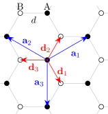
Figure 1. The honeycomb structure.

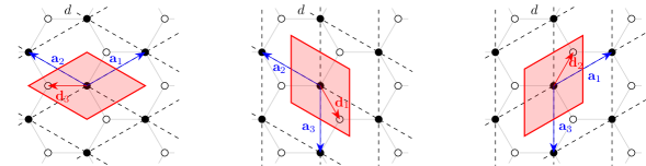
Figure 2. Three possible dimerizations of the honeycomb structure.

The vectors $\mathbf{a}_{i}$ generate a Bravais lattice $\Gamma:=\mathrm{Span}_{\mathbb{Z}}\{\mathbf{a}_{1},\mathbf{a}_{2},\mathbf{a}_{3}\}\cong\mathbb{Z}^{2}$ where one $\mathbf{a}_{i}$ is redundant as it is integer linear combination of the two others. Then any site of the crystal can be reached by a Bravais lattice vector and the use of one of the $\mathbf{d}_{i}$ vectors. It is then sufficient to pick two $\mathbf{a}_{i}$-vectors and one $\mathbf{d}_{i}$-vector to generate the whole crystal. This choice, which is often called a dimerization of $\mathcal{C}$, is not unique, as illustrated in Figure 2.

The above procedure is equivalent to the choice of a periodicity cell that contains two-non equivalent sites $A$ and $B$ (white and black dots in Figure 1), described as internal degrees of freedom besides the Bravais lattice. Hence, each choice of unit cell provides an isomorphism $\ell^{2}(\mathcal{C})\cong\ell^{2}(\mathbb{Z}^{2})\otimes\mathbb{C}^{2}$, leading to the Hilbert space $\mathcal{\mathcal{H}_{\mathrm{disc}}}$ (for $N=2$) discussed in Section 2, when the spin is taken into account.

A.2. The Hamiltonian. The Kane-Mele model is defined, in a first quantization formalism, by the Hamiltonian $H_{\mathrm{KM}}$, acting on $\ell^{2}(\mathcal{C})\otimes\mathbb{C}^{2}$ as

$$H_{\mathrm{KM}}=tH_{\mathrm{NN}}+\lambda_{v}H_{v}+\lambda_{\mathrm{SO}}H_{\mathrm{SO}}+\lambda_{\mathrm{R}}H_{\mathrm{R}}$$

where $t,\,\lambda_{v},\lambda_{\mathrm{SO}}$ and $\lambda_{\mathrm{R}}$ are real parameters corresponding to various physical effects. The first term is a nearest neighbor hopping term:

$$H_{\mathrm{NN}}=\sum_{i=1}^{3}\left(T_{\mathbf{d}_{i}}+T_{-\mathbf{d}_{i}}\right)\otimes\mathds{1}_{\mathbb{C}^{2}}$$

where $T_{\mathbf{u}}$ is a translation operator along vector $\mathbf{u}$, namely

$$(T_{\mathbf{u}}\psi)_{\mathbf{m}}=\begin{cases}\psi_{\mathbf{m}-\mathbf{u}}&\text{ if }{\mathbf{m}-\mathbf{u}}\in\mathcal{C};\\ 0&\text{ otherwise. }\end{cases}$$

The second term is a sublattice potential that distinguishes sites $A$ and $B$, namely

$$H_{v}=(\chi_{A}-\chi_{B})\otimes\mathds{1}_{\mathbb{C}^{2}}$$

for $\chi_{A}$ (resp. $\chi_{B}$) the characteristic function on the sublattice $A$ (resp. sublattice $B$) of $\mathcal{C}$. The third term is a spin-orbit term, corresponding to an effective and spin-dependent magnetic field due to an electric field inside the two-dimensional crystal. This is a next-to-nearest-neighbor term given by

$$H_{\mathrm{SO}}=-{\mathrm{i}}\left(\chi_{A}-\chi_{B}\right)\sum_{i=1}^{3}\left(T_{\mathbf{a}_{i}}-T_{-\mathbf{a}_{i}}\right)\otimes s_{z}.$$

Finally the last term is called a Rashba term. This is also a spin-orbit effect but due to an electric field orthogonal to the sample (for example in a heterostructure). This is a nearest-neighbor term given by

$$H_{\mathrm{R}}={\mathrm{i}}\big{(}T_{\mathbf{d}_{1}}-T_{-\mathbf{d}_{1}}\big{)}\otimes\Big{(}-\dfrac{\sqrt{3}s_{x}+s_{y}}{2}\Big{)}+{\mathrm{i}}\big{(}T_{\mathbf{d}_{2}}-T_{-\mathbf{d}_{2}}\big{)}\otimes\Big{(}\dfrac{\sqrt{3}s_{x}-s_{y}}{2}\Big{)}+{\mathrm{i}}\big{(}T_{\mathbf{d}_{3}}-T_{-\mathbf{d}_{3}}\big{)}\otimes s_{y}$$

Notice that this last term satisfies $[H_{\mathrm{R}},S_{z}]\neq 0$ so that $S_{z}$ and $H_{\mathrm{KM}}$ do not commute whenever $\lambda_{R}\neq 0$. Moreover, note that $H_{\mathrm{KM}}$ is periodic, since $[T_{\mathbf{u}_{1}},T_{\mathbf{u}_{2}}]=0$ for any vectors $\mathbf{u}_{1}$ and $\mathbf{u}_{2}$. In particular $H_{\mathrm{KM}}$ commutes with all the translation of the Bravais lattice $T_{\mathbf{\gamma}}$ for $\mathbf{\gamma}\in\Gamma$. It was also shown in [KM₁] that $H_{\mathrm{KM}}$ has a spectral gap for a wide region in parameter space, including $\lambda_{R}\neq 0$ (Figure 1 in [KM₁]).

In summary, $H_{\mathrm{KM}}$ is made of on-site ($H_{v}$), nearest-neighbor ($H_{\mathrm{NN}}$ and $H_{\mathrm{R}}$) and next to nearest-neighbor ($H_{\mathrm{SO}}$) terms. Note that after the dimerization procedure a nearest-neighbor term acts on internal degree of freedom, whereas next-to-nearest-neighbor exchange becomes simply nearest-neighbor. Thus, whatever the dimerization, one has

$$(H_{\mathrm{KM}})_{\mathbf{m},\mathbf{n}}=0\qquad\text{for}\qquad\left\|\mathbf{m}-\mathbf{n}\right\|_{1}>1$$

so that $H_{\mathrm{KM}}$ is trivially near-sighted. Indeed by adapting $C$ the inequality of Definition 2.1, $H_{\mathrm{KM}}$ is near-sighted for any range $\zeta>0$.

Appendix B From switch functions to position operators

In this Appendix, we re-elaborate some ideas and techniques which originally appeared in [AS²] in the continuum case ($\mathbb{R}^{2}$-covariant Schrödinger operators on the plane). We adapt their proof to the discrete case considered in this paper.

The crucial property of any switch function is the following one.

Lemma B.1.

Let $\Lambda_{j}$ be a switch function in the $j^{\mathrm{th}}$-direction for $j\in\left\{1,2\right\}$. Then, for every $n\in\mathbb{Z}$ one has

$$\sum_{m\in\mathbb{Z}}\left(\Lambda_{j}(m+n)-\Lambda_{j}(m)\right)=n.$$

Proof.

For $n=0$ the claim is trivial. Consider $n\geq 1$. Notice that the summand $\Lambda_{j}(m+n)-\Lambda_{j}(m)$ is non-zero only for finitely many $m\in\mathbb{Z}$. Hence,

$$\sum_{m\in\mathbb{Z}}\left(\Lambda_{j}(m+n)-\Lambda_{j}(m)\right) =\sum_{m\in\mathbb{Z}}\sum_{p=0}^{n-1}\big{(}\Lambda_{j}(m+(n-p))-\Lambda_{j}(m+(n-p-1))\big{)}$$ (B.1)

$$=\sum_{p=0}^{n-1}\sum_{m\in\mathbb{Z}}\big{(}\Lambda_{j}(m)-\Lambda_{j}(m-1)\big{)}.$$ (B.2)

Notice that $\sum_{m\in\mathbb{Z}}\big{(}\Lambda_{j}(m)-\Lambda_{j}(m-1)\big{)}=1$, since there is one and only one point $m\in\mathbb{Z}$ where the summand is not zero. This proves the statement for $n\geq 1$. The proof for $n\leq-1$ is analogous. ∎

For the sake of clarity, we recall that $\chi_{2,1}$ and $\chi_{1}$ are characteristic functions, respectively of the line $\left\{\mathbf{m}\in\mathbb{Z}^{2}:m_{2}=0\right\}$ and of the point $\left\{\mathbf{0}\right\}$.

Lemma B.2.

Let $A$, $B$ and $C$ be operators in $\mathcal{B}(\mathcal{H}_{\mathrm{disc}})$ which are periodic in the $2^{\mathrm{nd}}$-direction and let $\Lambda_{2}$ be a switch function in the $2^{\mathrm{nd}}$-direction. If $A[B,\Lambda_{2}]C$ is trace class, $A$ is $\alpha$-confined in the $1^{\mathrm{st}}$-direction, $C^{*}$ is $\beta$-confined in the $1^{\mathrm{st}}$-direction and $B$ satisfies

$$\mathcal{M}_{B}:=\max\left(\sup_{\mathbf{m}\in\mathbb{Z}^{2}}\sum_{n_{1}\in\mathbb{Z}}\left\lvert B_{\mathbf{m},(n_{1},0)}m_{2}\right\rvert,\sup_{n_{1}\in\mathbb{Z}}\sum_{\mathbf{m}\in\mathbb{Z}^{2}}\left\lvert B_{\mathbf{m},(n_{1},0)}m_{2}\right\rvert\right)<\infty,$$ (B.3)

then

$$\operatorname{Tr}(A[B,\Lambda_{2}]C)=-\operatorname{Tr}(AX_{2}B\chi_{2,1}C).$$

Proof.

Since $A[B,\Lambda_{2}]C$ is trace class, its trace can be computed through the diagonal kernel, and in view of the boundedness of $A$, $[B,\Lambda_{2}]$ and $C$, one has

$$\operatorname{Tr}(A[B,\Lambda_{2}]C)=\sum_{\mathbf{m}\in\mathbb{Z}^{2}}\sum_{\mathbf{n}\in\mathbb{Z}^{2}}\sum_{\mathbf{p}\in\mathbb{Z}^{2}}\operatorname{tr}\big{(}A_{\mathbf{m},\mathbf{n}}B_{\mathbf{n},\mathbf{p}}(\Lambda_{2}(p_{2})-\Lambda_{2}(n_{2}))C_{\mathbf{p},\mathbf{m}}\big{)}.$$ (B.4)

Now, notice that the function

$${\big{(}\mathbb{Z}^{2}\big{)}}^{3}\ni(\mathbf{m,n,p})\mapsto\operatorname{tr}\big{(}A_{\mathbf{m},\mathbf{n}}B_{\mathbf{n},\mathbf{p}}(\Lambda_{2}(p_{2})-\Lambda_{2}(n_{2}))C_{\mathbf{p},\mathbf{m}}\big{)}\text{ is in }\ell^{1}\big{(}{\big{(}\mathbb{Z}^{2}\big{)}}^{3}\big{)}.$$ (B.5)

Indeed, in view of the equivalence of norms on finite-dimensional vector spaces and the periodicity in the $2^{\mathrm{nd}}$-direction, first one notices that

$$\sum_{\mathbf{m}\in\mathbb{Z}^{2}}\sum_{\mathbf{n}\in\mathbb{Z}^{2}}\sum_{\mathbf{p}\in\mathbb{Z}^{2}}\left\lvert\operatorname{tr}\big{(}A_{\mathbf{m},\mathbf{n}}B_{\mathbf{n},\mathbf{p}}(\Lambda_{2}(p_{2})-\Lambda_{2}(n_{2}))C_{\mathbf{p},\mathbf{m}}\big{)}\right\rvert$$

$$\leq D_{1}\sum_{\mathbf{m}\in\mathbb{Z}^{2}}\sum_{\mathbf{n}\in\mathbb{Z}^{2}}\sum_{\mathbf{p}\in\mathbb{Z}^{2}}\left\lvert A_{\mathbf{m},\mathbf{n}}B_{\mathbf{n},\mathbf{p}}(\Lambda_{2}(p_{2})-\Lambda_{2}(n_{2}))C_{\mathbf{p},\mathbf{m}}\right\rvert$$

$$\leq\frac{D_{1}}{2}\sum_{\mathbf{m}\in\mathbb{Z}^{2}}\sum_{\mathbf{n}\in\mathbb{Z}^{2}}\sum_{\mathbf{p}\in\mathbb{Z}^{2}}\left\lvert B_{\mathbf{n},\mathbf{p}}\right\rvert\left\lvert(\Lambda_{2}(p_{2})-\Lambda_{2}(n_{2}))\right\rvert\big{(}\left\lvert A_{\mathbf{m},\mathbf{n}}\right\rvert^{2}+\left\lvert C_{\mathbf{p},\mathbf{m}}\right\rvert^{2}\big{)}$$

$$\leq\frac{D_{1}}{2}\sum_{\mathbf{n}\in\mathbb{Z}^{2}}\sum_{\mathbf{m}^{\prime}\in\mathbb{Z}^{2}}\sum_{\mathbf{p}^{\prime}\in\mathbb{Z}^{2}}\left\lvert B_{\mathbf{n},\mathbf{p}^{\prime}+(0,n_{2})}\right\rvert\left\lvert(\Lambda_{2}(p_{2}^{\prime}+n_{2})-\Lambda_{2}(n_{2}))\right\rvert\left\lvert A_{\mathbf{m}^{\prime}+(0,n_{2}),\mathbf{n}}\right\rvert^{2}+$$

$$\phantom{\leq}+\frac{D_{1}}{2}\sum_{\mathbf{p}\in\mathbb{Z}^{2}}\sum_{\mathbf{m}^{\prime}\in\mathbb{Z}^{2}}\sum_{\mathbf{n}^{\prime}\in\mathbb{Z}^{2}}\left\lvert B_{\mathbf{n}^{\prime}+(0,p_{2}),\mathbf{p}}\right\rvert\left\lvert(\Lambda_{2}(p_{2})-\Lambda_{2}(n_{2}^{\prime}+p_{2}))\right\rvert\left\lvert C_{\mathbf{p},\mathbf{m}^{\prime}+(0,p_{2})}\right\rvert^{2}$$

$$\leq\frac{D_{1}}{2}\sum_{\mathbf{n}\in\mathbb{Z}^{2}}\sum_{\mathbf{m}^{\prime}\in\mathbb{Z}^{2}}\sum_{\mathbf{p}^{\prime}\in\mathbb{Z}^{2}}\left\lvert B_{(n_{1},0),\mathbf{p}^{\prime}}\right\rvert\left\lvert(\Lambda_{2}(p_{2}^{\prime}+n_{2})-\Lambda_{2}(n_{2}))\right\rvert\left\lvert A_{\mathbf{m}^{\prime},(n_{1},0)}\right\rvert^{2}+$$

$$\phantom{\leq}+\frac{D_{1}}{2}\sum_{\mathbf{p}\in\mathbb{Z}^{2}}\sum_{\mathbf{m}^{\prime}\in\mathbb{Z}^{2}}\sum_{\mathbf{n}^{\prime}\in\mathbb{Z}^{2}}\left\lvert B_{\mathbf{n}^{\prime},(p_{1},0)}\right\rvert\left\lvert(\Lambda_{2}(p_{2})-\Lambda_{2}(n_{2}^{\prime}+p_{2}))\right\rvert\left\lvert C_{(p_{1},0),\mathbf{m}^{\prime}}\right\rvert^{2},$$

where $D_{1}$ is a constant. Then, one can estimates the right-hand side term of the last equation from above with

$$D_{1}D_{2}(\Lambda_{2})\Big{(}\sum_{n_{1}\in\mathbb{Z}}\sum_{\mathbf{m}^{\prime}\in\mathbb{Z}^{2}}\sum_{\mathbf{p}^{\prime}\in\mathbb{Z}^{2}}\left\lvert B_{(n_{1},0),\mathbf{p}^{\prime}}\right\rvert\left\lvert p_{2}^{\prime}\right\rvert\left\lvert A_{\mathbf{m}^{\prime},(n_{1},0)}\right\rvert^{2}+$$

$$\phantom{D_{1}D_{2}(\Lambda_{2})\Big{(}}+\sum_{p_{1}\in\mathbb{Z}}\sum_{\mathbf{m}^{\prime}\in\mathbb{Z}^{2}}\sum_{\mathbf{n}^{\prime}\in\mathbb{Z}^{2}}\left\lvert B_{\mathbf{n}^{\prime},(p_{1},0)}\right\rvert\left\lvert n_{2}^{\prime}\right\rvert\left\lvert C_{(p_{1},0),\mathbf{m}^{\prime}}\right\rvert^{2}\Big{)}$$

$$\leq D_{1}D_{2}(\Lambda_{2})\mathcal{M}_{B}\sum_{n_{1}\in\mathbb{Z},j\in\{1,\ldots,N\},s\in\{\uparrow,\downarrow\}}\big{(}\left\|A\left|(n_{1},0),j,s\right\rangle\right\|^{2}+\left\|C^{*}\left|(n_{1},0),j,s\right\rangle\right\|^{2}\big{)}$$

$$\leq D_{1}D_{2}(\Lambda_{2})\mathcal{M}_{B}\sum_{n_{1}\in\mathbb{Z},j\in\{1,\ldots,N\},s\in\{\uparrow,\downarrow\}}\big{(}\left\|A{\mathrm{e}}^{\alpha\left\lvert X_{1}\right\rvert}\right\|^{2}{\mathrm{e}}^{-2\alpha\left\lvert n_{1}\right\rvert}+\left\|C^{*}{\mathrm{e}}^{\beta\left\lvert X_{1}\right\rvert}\right\|^{2}{\mathrm{e}}^{-2\beta\left\lvert n_{1}\right\rvert}\big{)}<\infty,$$

where $D_{2}(\Lambda_{2})$ is a constant depending on $\Lambda_{2}$, we have used the hypotheses (B.3), and the fact that $A$ is $\alpha$-confined in the $1^{\mathrm{st}}$-direction and $C^{*}$ is $\beta$-confined in the $1^{\mathrm{st}}$-direction.

In view of (B.5) we can apply Fubini’s Theorem and, by Lemma B.1, we get that the right-hand side term of (B.4) reads

$$\sum_{p_{1}\in\mathbb{Z}}\sum_{\mathbf{m}^{\prime}\in\mathbb{Z}^{2}}\sum_{\mathbf{n}^{\prime}\in\mathbb{Z}^{2}}\operatorname{tr}\big{(}A_{\mathbf{m}^{\prime},\mathbf{n}^{\prime}}B_{\mathbf{n}^{\prime},(p_{1},0)}(-n_{2}^{\prime})C_{(p_{1},0),\mathbf{m}^{\prime}}\big{)}$$

$$=-\sum_{\mathbf{m}^{\prime}\in\mathbb{Z}^{2}}\operatorname{tr}\big{(}{(AX_{2}B\chi_{2,1}C)}_{\mathbf{m}^{\prime},\mathbf{m}^{\prime}}\big{)}.$$

Observe that by hypothesis (B.3) and Remark 4.1 (i), $X_{2}B\chi_{2,1}$ is bounded and thus $AX_{2}B\chi_{2,1}C$ is trace class, as $\chi_{2,1}C\in\mathcal{B}_{1}(\mathcal{H}_{\mathrm{disc}})$ by Proposition 4.7. Therefore, one concludes that

$$\operatorname{Tr}(A[B,\Lambda_{2}]C)=-\sum_{\mathbf{m}^{\prime}\in\mathbb{Z}^{2}}\operatorname{tr}\big{(}{(AX_{2}B\chi_{2,1}C)}_{\mathbf{m}^{\prime},\mathbf{m}^{\prime}}\big{)}=-\operatorname{Tr}(AX_{2}B\chi_{2,1}C).$$

∎

Lemma B.3.

Let $A$, $B$ and $C$ be periodic operators in $\mathcal{B}(\mathcal{H}_{\mathrm{disc}})$. Let $\Lambda_{1}$, $\Lambda_{2}$ be two switch functions, respectively in the $1^{\mathrm{st}}$ and $2^{\mathrm{nd}}$-direction. If $[A,\Lambda_{1}]B[C,\Lambda_{2}]$ is trace class and $A$ and $C$ satisfy

$$\sum_{\mathbf{n}\in\mathbb{Z}^{2}}\left\lvert A_{0,\mathbf{n}}n_{1}\right\rvert<\infty,\quad\sum_{\mathbf{n}\in\mathbb{Z}^{2}}\left\lvert C_{\mathbf{m},0}m_{2}\right\rvert<\infty,$$ (B.6)

then

$$\operatorname{Tr}([A,\Lambda_{1}]B[C,\Lambda_{2}])=-\operatorname{Tr}(\chi_{1}AX_{1}BX_{2}C\chi_{1}).$$

Proof.

Since $[A,\Lambda_{1}]B[C,\Lambda_{2}]$ is trace class, its trace can be computed through the diagonal kernel, and in view of boundedness of $[A,\Lambda_{1}]$, $B$ and $[C,\Lambda_{2}]$, one has

$$\operatorname{Tr}\Big{(}[A,\Lambda_{1}]B[C,\Lambda_{2}]\Big{)}$$

$$=\sum_{\mathbf{m}\in\mathbb{Z}^{2}}\sum_{\mathbf{n}\in\mathbb{Z}^{2}}\sum_{\mathbf{p}\in\mathbb{Z}^{2}}\operatorname{tr}\big{(}A_{\mathbf{m},\mathbf{n}}(\Lambda_{1}(n_{1})-\Lambda_{1}(m_{1}))B_{\mathbf{n},\mathbf{p}}C_{\mathbf{p},\mathbf{m}}(\Lambda_{2}(m_{2})-\Lambda_{1}(p_{2}))\big{)}.$$

Performing the change of variables $\mathbf{n}^{\prime}=\mathbf{n-m}$, $\mathbf{p}^{\prime}=\mathbf{p-m}$ and using the periodicity, one can rewrite the right-hand side term of the last equation as

$$\sum_{\mathbf{m}\in\mathbb{Z}^{2}}\sum_{\mathbf{n}^{\prime}\in\mathbb{Z}^{2}}\sum_{\mathbf{p}^{\prime}\in\mathbb{Z}^{2}}\operatorname{tr}\big{(}A_{\mathbf{m},\mathbf{n}^{\prime}+\mathbf{m}}(\Lambda_{1}(n_{1}^{\prime}+m_{1})-\Lambda_{1}(m_{1}))\cdot$$ (B.7)

$$\phantom{=}\cdot B_{\mathbf{n}^{\prime}+\mathbf{m},\mathbf{p}^{\prime}+\mathbf{m}}C_{\mathbf{p}^{\prime}+\mathbf{m},\mathbf{m}}(\Lambda_{2}(m_{2})-\Lambda_{1}(p_{2}^{\prime}+m_{2}))\big{)}=$$ (B.8)

$$=\sum_{\mathbf{m}\in\mathbb{Z}^{2}}\sum_{\mathbf{n}^{\prime}\in\mathbb{Z}^{2}}\sum_{\mathbf{p}^{\prime}\in\mathbb{Z}^{2}}\operatorname{tr}\big{(}A_{\mathbf{0},\mathbf{n}^{\prime}}(\Lambda_{1}(n_{1}^{\prime}+m_{1})-\Lambda_{1}(m_{1}))\cdot$$ (B.9)

$$\phantom{=}\cdot B_{\mathbf{n}^{\prime},\mathbf{p}^{\prime}}C_{\mathbf{p}^{\prime},\mathbf{0}}(\Lambda_{2}(m_{2})-\Lambda_{1}(p_{2}^{\prime}+m_{2}))\big{)}.$$ (B.10)

In view of the equivalence of norms on finite-dimensional vector spaces and hypothesis (B.6), one has

$$\sum_{\mathbf{m}\in\mathbb{Z}^{2}}\sum_{\mathbf{n}^{\prime}\in\mathbb{Z}^{2}}\sum_{\mathbf{p}^{\prime}\in\mathbb{Z}^{2}}\left\lvert\operatorname{tr}\big{(}A_{\mathbf{0},\mathbf{n}^{\prime}}(\Lambda_{1}(n_{1}^{\prime}+m_{1})-\Lambda_{1}(m_{1}))B_{\mathbf{n}^{\prime},\mathbf{p}^{\prime}}C_{\mathbf{p}^{\prime},\mathbf{0}}(\Lambda_{2}(m_{2})-\Lambda_{1}(p_{2}^{\prime}+m_{2}))\big{)}\right\rvert$$

$$\leq D_{1}\sum_{\mathbf{n}^{\prime}\in\mathbb{Z}^{2}}\sum_{\mathbf{p}^{\prime}\in\mathbb{Z}^{2}}\left\lvert A_{\mathbf{0},\mathbf{n}^{\prime}}\right\rvert\sum_{m_{1}\in\mathbb{Z}}\left\lvert\Lambda_{1}(n_{1}^{\prime}+m_{1})-\Lambda_{1}(m_{1})\right\rvert\cdot$$

$$\phantom{\leq}\cdot\left\lvert B_{\mathbf{n}^{\prime},\mathbf{p}^{\prime}}C_{\mathbf{p}^{\prime},\mathbf{0}}\right\rvert\sum_{m_{2}\in\mathbb{Z}}\left\lvert\Lambda_{2}(m_{2})-\Lambda_{1}(p_{2}^{\prime}+m_{2})\right\rvert$$

$$\leq D_{1}\left\|B\right\|D_{2}(\Lambda_{1})D_{3}(\Lambda_{2})\sum_{\mathbf{n}^{\prime}\in\mathbb{Z}^{2}}\left\lvert A_{\mathbf{0},\mathbf{n}^{\prime}}\right\rvert\left\lvert n_{1}^{\prime}\right\rvert\sum_{\mathbf{p}^{\prime}\in\mathbb{Z}^{2}}\left\lvert C_{\mathbf{p}^{\prime},\mathbf{0}}\right\rvert\left\lvert p_{2}^{\prime}\right\rvert<\infty,$$

where $D_{1}\in\mathbb{R}$, $D_{2}(\Lambda_{1}),D_{3}(\Lambda_{2})$ are constants depending respectively on $\Lambda_{1},\Lambda_{2}$. Therefore, applying Fubini’s Theorem and Lemma B.1, one can rewrite the right-hand side term of (B.7) as

$$\sum_{\mathbf{n}^{\prime}\in\mathbb{Z}^{2}}\sum_{\mathbf{p}^{\prime}\in\mathbb{Z}^{2}}\operatorname{tr}\big{(}A_{\mathbf{0},\mathbf{n}^{\prime}}n_{1}^{\prime}B_{\mathbf{n}^{\prime},\mathbf{p}^{\prime}}(-p_{2}^{\prime})C_{\mathbf{p}^{\prime},\mathbf{0}}\big{)}=-\sum_{\mathbf{m}\in\mathbb{Z}^{2}}\operatorname{tr}\big{(}{(\chi_{1}AX_{1}BX_{2}C\chi_{1})}_{\mathbf{m},\mathbf{m}}\big{)}$$

Observe that by hypothesis (B.6) and Remark 4.1 (i), $\chi_{1}AX_{1}$ and $X_{2}C\chi_{1}$ are bounded and thus $\chi_{1}AX_{1}BX_{2}C\chi_{1}$ is trace class. Therefore, one concludes that

$$\operatorname{Tr}\Big{(}[A,\Lambda_{1}]B[C,\Lambda_{2}]\Big{)}=-\sum_{\mathbf{m}\in\mathbb{Z}^{2}}\operatorname{tr}\big{(}{(\chi_{1}AX_{1}BX_{2}C\chi_{1})}_{\mathbf{m},\mathbf{m}}\big{)}=-\operatorname{Tr}(\chi_{1}AX_{1}BX_{2}C\chi_{1}).$$

∎

(G. Marcelli)	Dipartimento di Matematica, “La Sapienza” Università di Roma
	Piazzale Aldo Moro 2, 00185 Rome, Italy
	E-mail address: marcelli@mat.uniroma1.it
(G. Panati)	Dipartimento di Matematica, “La Sapienza” Università di Roma
	Piazzale Aldo Moro 2, 00185 Rome, Italy
	E-mail address: panati@mat.uniroma1.it
(C. Tauber)	Institute for Theoretical Physics, ETH Zürich
	Wolfgang-Pauli-Str. 27, CH-8093 Zürich, Switzerland
	E-mail address: tauberc@phys.ethz.ch

References

- [ALLL] An, Z.; Liu, F. Q.; Lin, Y.; Liu, C. : The universal definition of spin current. Scientific reports 2, 388 (2012).
- [An] Ando, Y. : Topological insulator materials, J. Phys. Soc. Jpn. 82 (2013), 102001.
- [AG] Aizenman, M.; Graf G.M. : Localization bounds for an electron gas, J. Phys. A: Math. Gen. 31(32), 6783 (1998).
- [AW] Aizenman, M.; Warzel, S. : Random Operators. Graduate Studies in Mathematics 168, American Methematical Society, United States of America, 2015.
- [ASV] Avila, J.C.; Schulz-Baldes, H.; Villegas-Blas, C. : Topological invariants of edge states for periodic two-dimensional models, Mathematical Physics, Analysis and Geometry 16, 136–170 (2013).
- [AS] Avron, J. E.; Seiler, R. : Quantization of the Hall conductance for general, multiparticle Schrödinger Hamiltonians. Phys. Rev. Lett. 54, 259–262 (1985).
- [AS2] Avron, J.; Seiler, R.; Simon, B. : Charge Deficiency, Charge Transport and Comparison of Dimensions, Commun. Math. Phys. 159, 399–422 (1994).
- [BGKS] Bouclet, J.M.; Germinet, F.; Klein, A.; Schenker, J.H. : Linear response theory for magnetic Schrödinger operators in disordered media, J. Funct. Analysis 226, 301–372 (2005).
- [BN] Bray-Ali, N.; Nussinov, Z. : Conservation and persistence of spin currents and their relation to the Lieb-Schulz-Mattis twist operators. Phys. Rev. B 80, 012401 (2009).
- [CDFG] Carpentier, D.; Delplace, P.; Fruchart, M.; Gawedzki, K. : Topological index for periodically driven time-reversal invariant 2D systems, Phys. Rev. Lett. 114, 106806 (2015).
- [CDFGT] Carpentier, D.; Delplace, P.; Fruchart, M.; Gawedzki, K.; Tauber, C. : Construction and properties of a topological index for periodically driven time-reversal invariant 2D crystals, Nuclear Physics B 896 779-834 (2015)
- [CMT] Cornean, H. D.; Monaco, D.; Teufel, S. : Wannier functions and invariants in time-reversal symmetric topological insulators. Rev. Math. Phys. 29, 1730001 (2017).
- [DG] De Nittis, G.; Gomi, K. : Classification of “Quaternionic” Bloch-Bundles. Commun. Math. Phys. 339, 1-55, (2015).
- [EGS] Elgart, A.; Graf, G.M.; Schenker, J.H. : Equality of the bulk and edge Hall conductances in a mobility gap, Commun. Math. Phys. 259(1), 185–221 (2005).
- [ES] Elgart, A.; Schlein, B. : Adiabatic Charge Transport and the Kubo Formula for Landau-Type Hamiltonians. Comm. Pure Appl. Math. 57, 590–615 (2004).
- [FMP] Fiorenza, D.; Monaco, D.; Panati, G. : Invariants of Topological Insulators as Geometric Obstructions. Commun. Math. Phys. 343, 1115-1157 (2016).
- [FW] Fröhlich, J. ; Werner, Ph. : Gauge theory of topological phases of matter, EPL 101, 47007 (2013).
- [FK] Fu, L.; Kane, C.L. : Time reversal polarization and a adiabatic spin pump, Phys. Rev. B 74, 195312 (2006).
- [FKM] Fu, L.; Kane, C.L.; Mele, E.J. : Topological insulators in three dimensions, Phys. Rev. Lett. 98, 106803 (2007).
- [Ga] Gawedzki, K. : Square root of gerbe holonomy and invariants of time-reversal-symmetric topological insulators, J. Geom. Phys. 120, 169-191 (2017).
- [Gr] Graf, G.M. : Aspects of the Integer Quantum Hall Effect, Proceedings of Symposia in Pure Mathematics 76, 429–442 (2007).
- [GP] Graf, G.M.; Porta, M. : Bulk-edge correspondence for two-dimensional topological insulators, Commun. Math. Phys. 324, 851–895 (2013).
- [Hal] Haldane, F.D.M. : Model for a Quantum Hall Effect without Landau levels: condensed-matter realization of the “parity anomaly”, Phys. Rev. Lett. 61, 2017 (1988).
- [HK] Hasan, M.Z.; Kane, C.L. : Colloquium: Topological Insulators, Rev. Mod. Phys. 82, 3045–3067 (2010).
- [KM1] Kane, C.L.; Mele, E.J. : Topological Order and the Quantum Spin Hall Effect, Phys. Rev. Lett. 95, 146802 (2005).
- [KM2] Kane, C.L.; Mele, E.J. : Quantum Spin Hall Effect in graphene, Phys. Rev. Lett. 95, 226801 (2005).
- [KK] Katsura, H.; Koma, T. The index of disordered topological insulators with time reversal symmetry. J. Math. Phys. 57(2), 021903, (2016).
- [Kir] Kirsch, W. : An invitation to random Schrödinger operators, preprint available at arXiv:0709.3707
- [Kit] Kitaev, A. : Periodic table for topological insulators and superconductors, AIP Conf. Proc. 1134, 22 (2009).
- [Ko] Kohn, W. : Density functional and density matrix method scaling linearly with the number of atoms, Phys. Rev. Lett. 76(17), 3168 (1996).
- [Ma] Marcelli, G. : A Mathematical Analysis of Spin and Charge Transport in Topological Insulators, Ph.D. thesis in Mathematics, “La Sapienza” Universitá di Roma, Rome, 2017.
- [MMPTe] Marcelli, G.; Monaco, D.; Panati, G.; Teufel, S. : Kubo formula for the Quantum Spin Hall conductivity: a microscopic derivation, in preparation (2018).
- [MPTa] Marcelli, G.; Panati, G.; Tauber, C. : Quantum Spin Hall conductance: Kubo formula and beyond, in preparation (2018).
- [MP] Monaco, D.; Panati, G. : Symmetry and localization in periodic crystals: triviality of Bloch bundles with a fermionic time-reversal symmetry, to appear in Acta App. Math. (2015).
- [MT] Monaco, D. ; Tauber, C. : Gauge-theoretic invariants for topological insulators: a bridge between Berry, WessÐZumino, and FuÐKaneÐMele. Lett. Math. Phys., 107, 1315–1343 (2017).
- [MB] Moore, J.E.; Balents, L. : Topological invariants of time-reversal-invariant band structures, Phys. Rev. B 75, 121306(R) (2007).
- [Mu] Murakami, S. : Quantum spin Hall effect and enhanced magnetic response by spin-orbit coupling. Phys. Rev. Lett. 97, 236805 (2006).
- [Pa] Panati, G.: Triviality of Bloch and Bloch-Dirac bundles, Ann. Henri Poincaré 8, 995–1011 (2007).
- [PK] Prodan, E.; Kohn, W. : Nearsightedness of electronic matter, Proc. Natl. Acad. Sci. U.S.A. 102, 11635–11638 (2005).
- [Pr1] Prodan, E. : Robustness of the Spin-Chern number, Phys. Rev. B 80, 125327 (2009).
- [Pr3] Prodan, E. : Manifestly gauge-independent formulations of the invariants, Phys. Rev. B 83, 235115 (2011).
- [RS1] Reed, M.; Simon, B. : Methods of Modern Mathematical Physics I: Functional Analysis. Academic Press, New York, (1979).
- [RF] Royden, H.L.; Fitzpatrick, P.M. : Real Analysis. Prentice Hall, United States of America, (2010).
- [RSFL] Ryu, S.; Schnyder, A.P.; Furusaki, A.; Ludwig, A.W.W. : Topological insulators and superconductors: Tenfold way and dimensional hierarchy, New J. Phys. 12, 065010 (2010).
- [Sch1] Schulz-Baldes, H. : Persistence of spin edge currents in disordered Quantum Spin Hall systems, Commun. Math. Phys. 324, 589–600 (2013).
- [Sch2] Schulz-Baldes, H. : -indices and factorization properties of odd symmetric Fredholm operators, Doc. Math. 20, 1481–1500 (2015).
- [SZXN] Shi, J.; Zhang, P.; Xiao, D.; Niu, Q. : Proper definition of spin current in spin-orbit coupled systems. Phys. Rev. Lett. 96, 076604 (2006).
- [Si] Simon, B. : Trace Ideals and their Applications, American Mathematical Society, 2005.
- [SXW] Sun, Q. F.; Xie, X. C.; Wang, J. : Persistent spin current in nano-devices and definition of the spin current. Phys. Rev. B 77, 035327 (2008).
- [TKNN] Thouless, D.J.; Kohmoto, M.; Nightingale, M.P.; de Nijs, M. : Quantized Hall conductance in a two-dimensional periodic potential, Phys. Rev. Lett. 49, 405–408 (1982).
- [ZWSXN] Zhang, P.; Wang, Z.; Shi, J.; Xiao, D.; Niu, Q. : Theory of conserved spin current and its application to a two-dimensional hole gas. Phys. Rev. B 77, 075304 (2008).