Monte Carlo modified profile likelihood
in models for clustered data

Abstract

The main focus of the analysts who deal with clustered data is usually not on the clustering variables, and hence the group-specific parameters are treated as nuisance. If a fixed effects formulation is preferred and the total number of clusters is large relative to the single-group sizes, classical frequentist techniques relying on the profile likelihood are often misleading. The use of alternative tools, such as modifications to the profile likelihood or integrated likelihoods, for making accurate inference on a parameter of interest can be complicated by the presence of nonstandard modelling and/or sampling assumptions. We show here how to employ Monte Carlo simulation in order to approximate the modified profile likelihood in some of these unconventional frameworks. The proposed solution is widely applicable and is shown to retain the usual properties of the modified profile likelihood. The approach is examined in two instances particularly relevant in applications, i.e. missing-data models and survival models with unspecified censoring distribution. The effectiveness of the proposed solution is validated via simulation studies and two clinical trial applications.

1 Introduction

Clustered data, either cross-sectional or longitudinal observations which may be arranged in groups, are nowadays encountered in all applied areas. Their main characteristic is the unobserved heterogeneity across clusters, with the consequence that units within a cluster might be correlated. How to deal with such correlation depends strongly on the purpose of the study. When the interest is on group-specific effects and also on estimation of the intra-cluster correlation, a frequent practice is to assume a random effects model. In this setting, cluster-specific covariate effects depend on unobservable latent variables, named random effects. Such a modelling strategy leads to the so-called conditional approach. Alternatively, if the interest centers on comparing the response variable of units across groups, it is preferable to adopt so-called marginal models, where the clustering structure is ignored for estimation of the regression coefficients, and it is only employed to ensure correct inference on the standard errors. These specifications are usually estimated using generalized estimating equations (Liang and Zeger, 1986). Generally, interpretation of the regression coefficients in conditional and marginal models is different. Therefore the corresponding estimates are not directly comparable (see, for instance, Lee and Nelder, 2004, and Agresti, 2015, Chapter 9). In this paper, we will focus mainly on the conditional approach.

Random effects models require to assume some suitable underlying distribution for the random effects, and even their incorrelation with the covariates in the model (Lancaster, 2000). The latter unrealistic hypothesis frequently drives the decision to opt for a more flexible fixed effects approach, a choice particularly popular in the econometric literature. Fixed effects models capture the heterogeneity among clusters via the inclusion of nuisance parameters, one for every group. These are also referred to as incidental parameters (Lancaster, 2000), since each of them appears only in the distribution of the observations in one given cluster. Under fixed effects models, as well as under marginal models, inferential results are free from any assumption on the probabilistic distribution regarding the dependence structure within clusters. In addition, if also relevant for the analysis, the fixed effects strategy allows to quantify the heterogeneity across groups by comparing the estimates of the cluster-specific parameters.

The increased robustness of the fixed effects solution over the random effects one in the conditional approach is balanced by the drawback that when clusters have small to moderate size, likelihood inference is prone to suffer from the incidental parameters problem (Neyman and Scott, 1948). Such problem depends on the fact that the bias of the profile score function for the parameter of interest increases along with the dimension of the nuisance component in the model (see, e.g., McCullagh and Tibshirani, 1990), invalidating usual asymptotic results if the number of groups, $N$, is much larger than the single group size, $T$. Reliable inference on the parameter of interest needs thus to be carried out via alternative pseudo-likelihoods which are unaffected by this issue.

Exact pseudo-likelihoods leading to extremely accurate conclusions are only available in specific model classes (Severini, 2000, Chapter 8). Correcting the profile likelihood for the presence of incidental parameters represents instead a more general strategy. Among the several adjustments found in the literature, a prominent position is held by the modified profile likelihood (MPL) of Barndorff-Nielsen (1980, 1983). Specifically, Sartori (2003) proved its inferential superiority with respect to the ordinary profile likelihood within the $(T\times N)$-asymptotic setting that characterizes clustered data with independent units.

Under the same frequentist paradigm, another possible approach to avoid the incidental parameters problem is the integrated likelihood for the component of interest (Severini, 2007), where elimination of the fixed effects is achieved by integration in an appropriate parametrization. De Bin et al. (2015) have shown that this function is asymptotically equivalent to the MPL and enjoys analogue properties in the two-index asymptotics for clustered data.

The first formulation of the MPL involves statistical quantities which are easily obtainable only for exponential or group family models (Pace and Salvan, 1997, Chapters 5, 7). Such computational difficulties can be overcome by the approximate MPL owed to Severini (1998) just within a limited range of statistical problems. Bartolucci et al. (2016) use Monte Carlo simulation in order to compute Severini’s version of the MPL when its exact calculation, although possible in principle, is especially tedious, given the assumed dependence structure of the data. The same complication arises under the nonstationary autoregressive model for normally distributed observations, discussed in (De Bin et al., 2015, Example 4.3) as an example of application for the integrated likelihood. In the Supplementary material, it is possible to see how the MPL can be conveniently computed via Monte Carlo simulation even in that setting.

The aim of this paper is to extend the Monte Carlo approach to situations where the analytical calculation of the MPL is not only tedious, but can also be infeasible due to peculiar modelling and/or sampling hypotheses. We illustrate the potential usefulness of the method in two frameworks highly relevant for applications. In particular, the first considers binary regression with nonignorable missing response, while the second deals with survival data with unspecified censoring distribution. In both cases, although not directly covered by the theory in Sartori (2003), the usual good inferential properties of the MPL are empirically confirmed, suggesting the proposed Monte Carlo solution as the default choice in applications.

The structure of the paper is as follows. Section 2 introduces the basic notation and defines the profile and modified profile log-likelihoods in models for clustered data. The procedure for computing the MPL through Monte Carlo approximation is detailed in Section 3, and then its use is illustrated by means of simulations in different nonstandard contexts for grouped observations. In particular, datasets with possibly missing binary response are considered by Section 4, whereas Section 5 is dedicated to survival data with unspecified censoring mechanism. The issues related to the calculation of the MPL are ascribable to the model complexity implied by the incompleteness of the data in the first case, and to the lack of parametric assumptions on the distribution of the censoring times in the second. In both frameworks we also consider an application to clinical trial data that illustrates the practical effectiveness of the method. Main results are summarised and commented in Section 6, which also mentions potential developments of the present work.

2 Profile and modified profile likelihood

For clustered observations $y_{it}$ subdivided in $N$ groups of sizes $T_{i}$, suppose the parametric statistical model

$$Y_{it}|X_{it}=x_{it}\sim p(y_{it}|x_{it};\psi,\lambda_{i})\,,\qquad i=1,\dots,N,\ \ \;t=1,\dots,T_{i},$$ (1)

which accommodates also dynamic specifications where the index $t$ runs over consecutive time periods and the temporal evolution of the dependent variable is explained by including in the $p$-dimensional vector of covariates $x_{it}$ responses previously recorded in the same cluster (see Section S2 of the Supplementary material). The global parameter is $\theta=(\psi,\lambda)$, where $\psi\in\Psi\subseteq{\rm I}\negthinspace{\rm R}^{k}$ denotes the component of interest and $\lambda=(\lambda_{1},\ldots,\lambda_{N})\in\Lambda$ indicates the vector containing the incidental parameters. Note that, here and henceforth, in order to avoid clutter we omit the transpose symbol acting on vectors unless such an omission could result in ambiguity. In the following, the assumptions of balanced groups and scalar nuisance components, i.e. $T_{i}=T$ and dim$(\lambda_{i})=1$ for each $i=1,\ldots,n$, respectively, shall be used without loss of generality, for the sake of notational simplicity only.

Under the hypothesis of independent groups, the log-likelihood function about $\theta$ can be expressed by

$$l(\theta)=\sum_{i=1}^{N}l^{i}(\theta)=\sum_{i=1}^{N}l^{i}(\psi,\lambda_{i})\,,$$

with $l^{i}(\psi,\lambda_{i})=\sum_{t=1}^{T}\log p(y_{it}|x_{it};\psi,\lambda_{i})$ being the log-likelihood contribution for the $i$th cluster. Let us define the full maximum likelihood (ML) estimate for model (1) as $\hat{\theta}=(\hat{\psi},\hat{\lambda})=\arg\max_{\theta}l(\theta)$. Standard likelihood inference on the parameter of interest is typically based on the profile log-likelihood

$$l_{P}(\psi)=\sum_{i=1}^{N}l^{i}\big{(}\psi,\hat{\lambda}_{i\psi}\big{)}=\sum_{i=1}^{N}l^{i}_{P}(\psi)\,,$$ (2)

where $\hat{\lambda}_{i\psi}$ is the constrained ML estimate of $\lambda_{i}$ for fixed $\psi$ obtained, under standard regularity conditions, by equating to zero the score

$$l_{\lambda_{i}}(\theta)=\frac{\partial l^{i}(\psi,\lambda_{i})}{\partial\lambda_{i}}$$ (3)

and solving for $\lambda_{i}$ $(i=1,\dots,N)$. Given $\hat{\lambda}_{\psi}=(\hat{\lambda}_{1\psi},\dots,\hat{\lambda}_{N\psi})$, the full constrained ML estimate for fixed $\psi$ is denoted by $\hat{\theta}_{\psi}=(\psi,\hat{\lambda}_{\psi})$.

The general expression taken by the logarithmic version of the MPL is

$$l_{M}(\psi)=l_{P}(\psi)+M(\psi)\,,$$ (4)

where the modification term $M(\psi)$ serves to remedy the effect of replacing the unknown nuisance parameter $\lambda$ with the estimate $\hat{\lambda}_{\psi}$ in the profile likelihood. Such plug-in effect typically translates in bias of the profile score function. The expression of $M(\psi)$ largely corrects this bias, making the MPL much closer to a proper likelihood (McCullagh and Tibshirani, 1990; Diciccio et al., 1996).

The independence hypothesis among clusters implies the additive form $M(\psi)=\sum_{i=1}^{N}M_{i}(\psi)$. By using Severini’s formulation of the MPL (Severini, 1998), the $i$th summand in the modification term equals

$$M_{i}(\psi)=\frac{1}{2}\log j_{\lambda_{i}\lambda_{i}}(\hat{\theta}_{\psi})-\log I_{\lambda_{i}\lambda_{i}}(\hat{\theta};\hat{\theta}_{\psi})\,,\qquad i=1,\dots,N.$$ (5)

In (5), $j_{\lambda_{i}\lambda_{i}}(\theta)=-\partial^{2}l^{i}(\psi,\lambda_{i})/(\partial\lambda_{i}\partial\lambda_{i})$ is evaluated at the constrained ML estimate $\hat{\theta}_{\psi}$ and $I_{\lambda_{i}\lambda_{i}}(\hat{\theta};\hat{\theta}_{\psi})$ is an approximation of a term involving sample space derivatives in the original Barndorff-Nielsen’s MPL. In particular, $I_{\lambda_{i}\lambda_{i}}(\hat{\theta};\hat{\theta}_{\psi})=E_{\theta_{0}}\big{\{}l_{\lambda_{i}}(\theta_{0})l_{\lambda_{i}}(\theta_{1})\big{\}}\big{|}_{\theta_{0}=\hat{\theta},\theta_{1}=\hat{\theta}_{\psi}}$ indicates the scalar expected value calculated with regard to the full ML estimate $\hat{\theta}$ of the product of partial score functions defined in (3) evaluated at two different points in the parameter space, i.e. $\hat{\theta}$ and $\hat{\theta}_{\psi}$. In contrast to the original formulation introduced by Barndorff-Nielsen (1980, 1983), Severini’s variant of $M(\psi)$ is computable even when the conditional probability density or mass function of $y_{it}$ given $x_{it}$ does not belong to full exponential or composite group families.

Sartori (2003) gives sufficient conditions under which inferences on $\psi$ conducted via the profile or the modified profile likelihood are adequate when dealing with independent clustered data. In more detail, usual results apply in the $(T\times N)$-asymptotics for quantities based on $l_{P}(\psi)$ if $N=o(T)$, while it suffices that $N=o(T^{3})$ to achieve reliable conclusions using the MPL in (4). This explains why the employment of $l_{M}(\psi)$ should be preferred in the presence of highly stratified datasets where the quantity of groups is much larger than the amount of observations per group.

3 Monte Carlo modified profile likelihood

Analytical computation of (5) is fairly simple in a number of widespread statistical models (see, e.g., Bellio and Sartori, 2003, and Bellio and Sartori, 2006). However, the expected value $I_{\lambda_{i}\lambda_{i}}(\hat{\theta};\hat{\theta}_{\psi})$ cannot be readily obtained in circumstances that demand special assumptions to correctly model the relevant aspects of the phenomenon under study. Sometimes its exact calculation is too cumbersome, sometimes infeasible.

One convenient expedient to compute Severini’s MPL even when the necessary expectation is not available in closed form foresees to approximate $I_{\lambda_{i}\lambda_{i}}(\hat{\theta};\hat{\theta}_{\psi})$ by the following empirical quantity based on $R$ Monte Carlo replicates:

$$I^{*}_{\lambda_{i}\lambda_{i}}(\hat{\theta};\hat{\theta}_{\psi})=\dfrac{1}{R}\sum_{r=1}^{R}l^{r}_{\lambda_{i}}(\hat{\theta})l^{r}_{\lambda_{i}}(\hat{\theta}_{\psi})\,,\qquad i=1,\dots,N,$$ (6)

where $l^{r}_{\lambda_{i}}(\cdot)$ is the score (3) computed on observations $y_{it}^{r}$ of the $r$th sample $(r=1,\dots,R)$ randomly generated under the ML fit of model (1), thus setting $(\psi,\lambda)=(\hat{\psi},\hat{\lambda})$. It is worth mentioning that such a strategy only requires to derive the score function $l_{\lambda_{i}}(\theta)$ and to simulate from the assumed distribution of the data, with no additional fitting. Indeed, $\hat{\theta}$ and $\hat{\theta}_{\psi}$ in (6) are the estimates derived from the observed dataset. This makes the approximation far less expensive than a standard bootstrap from a computational standpoint. Moreover, the execution time is not particularly influenced by the value of $T$ and the number of replications $R$ usually does not need to exceed 500 for a reasonably accurate estimation of $\psi$, as attested by preliminary sensitivity analyses.

The principal quality of this Monte Carlo solution is its broad applicability. Bartolucci et al. (2016) already experimented it, proving its competitiveness with econometric inferential methods in the estimation of dynamic fixed effects models for binary panel data. Here, we propose to adopt and extend the same technique in order to investigate the superiority of $l_{M}(\psi)$ with respect to ML procedures in alternative scenarios. To this end, we will consider regression models for missing binary data (Section 4) and survival models for right-censored data (Section 5), two practically relevant settings in which explicit formulation of (5) is either computationally involving or impossible due to the particular modelling framework. Specifically, in the survival analysis case we will use a fitted semiparametric model for generating the Monte Carlo samples to calculate (6), making inference robust with respect to a possibly misspecified censoring distribution.

For ease of reference, from now on Severini’s version of the MPL obtained by making use of Monte Carlo simulation will be called Monte Carlo MPL (MCMPL). The corresponding log-likelihood function is $l_{M^{*}}(\psi)=l_{P}(\psi)+M^{*}(\psi)$, where the modification term takes the form

$$M^{*}(\psi)=\sum_{i=1}^{N}M^{*}_{i}(\psi)=\sum_{i=1}^{N}\bigg{\{}\frac{1}{2}\log j_{\lambda_{i}\lambda_{i}}(\hat{\theta}_{\psi})-\log I^{*}_{\lambda_{i}\lambda_{i}}(\hat{\theta};\hat{\theta}_{\psi})\bigg{\}}\,,$$

with $I^{*}_{\lambda_{i}\lambda_{i}}(\hat{\theta};\hat{\theta}_{\psi})$ defined in (6).

Generally, both $l_{P}(\psi)$ and $l_{M^{*}}(\psi)$ are maximized numerically. Of course, the higher the dimension of $\psi$, the larger the number of iterations for the numerical optimization could be. Nevertheless, for fixed $R$, the overall computational effort required by $l_{M^{*}}(\psi)$ increases linearly with the number of iterations and, in our experience, hardly becomes too costly with respect to $l_{P}(\psi)$.

4 Regression models for missing binary data

4.1 Introduction

The lacking registration of some data is the rule rather than the exception in quantitative research analysis. Rubin (1976) developed the first basic classification of data still in use today: missing completely at random (MCAR), missing at random (MAR) and missing not at random (MNAR). While the first two categories are associated with an ignorable mechanism of missingness, when data are MNAR the probability of missing observations also depends on values that are unobserved, and thus the supposed model must take into account the missingness process for providing valid results (Little and Rubin, 2002, Section 15.1).

Among the various approaches proposed to deal with the nonignorable incompleteness of the data, selection models and pattern-mixture models play a major role (Fitzmaurice et al., 2008, Chapter 18). Let us consider independent possibly missing clustered observations $y_{it}$ and define the corresponding missingness indicators $M_{it}$ such that $M_{it}=1$ if $y_{it}$ is unobserved and $M_{it}=0$ otherwise $(i=1,\ldots,N,t=1,\dots,T)$. From a likelihood viewpoint, the joint distribution of $Y_{it}$ and $M_{it}$ in some global parametrization $\varphi$ has to be specified. Following the classical formulation of selection models, we shall assume a marginal distribution for $Y_{it}$ depending on the parameter $\theta$ and a conditional distribution of $M_{it}$ given $Y_{it}=y_{it}$ depending on $\gamma$, so that

$$p_{Y,M}(y_{it},m_{it}|x_{it};\varphi)=p_{Y}(y_{it}|x_{it};\theta)p_{M|Y}(m_{it}|y_{it},x_{it};\gamma)\,,$$ (7)

with $\varphi=(\theta,\gamma)$.

Computationally speaking, in moderately complex models for incomplete datasets, maximization of the log-likelihood function incorporating all the available information is often quite an arduous task. Indeed this function, named observed log-likelihood, involves integrals or summations over the distribution of the missing data which can be hardly tractable. It is well-known that the EM algorithm (Dempster et al., 1977) is a possibly advantageous strategy for ML estimation whenever data either are partially not observed or may be viewed as such. This method is pervasive in the literature of missing data, and many extensions to the original version have been posited in the years (Little and Rubin, 2002, Section 8.5). Optimization problems in likelihood inference may also be solved by numerical iterative algorithms different from the EM. For example, we recall the Nelder-Mead simplex method (Nelder and Mead, 1965) applied by Troxel et al. (1998) and Troxel et al. (1998) in presence of arbitrarily MNAR clustered observations, and the popular Newton-Raphson algorithm employed by both Parzen et al. (2006) and Sinha et al. (2011).

A universally optimal solution to maximize the log-likelihood in studies with incomplete observations is impossible to prescribe. It is yet important to point out that, regardless of the selected technique, nonignorable missing-data models need to be fitted with special care because the available information may be insufficient to estimate all parameters (Ibrahim et al., 2001).

4.2 Setup and Monte Carlo modified profile likelihood

We focus here on possibly missing clustered binary observations. Adopting the typical factorization of selection models defined in (7), for independent data $y_{it}$ one can write the marginal probability mass function

$$Y_{it}\sim Bern(\pi_{it}),\;\pi_{it}=\pi_{it}(\theta)=F(\lambda_{i}+\beta^{\mathrm{T}}x_{it})\,,\;i=1,\dots,N,\ t=1,\dots,T,$$ (8)

with $F(\cdot)$ a suitable cumulative distribution function (CDF) and $\beta=(\beta_{1},\ldots,\beta_{p})$ vector of regression parameters, whereas the conditional model for the missingness indicator introduced in Section 4.1 may be expressed by

$$M_{it}|Y_{it}=y_{it}\sim Bern(\zeta_{it})\,,\qquad i=1,\dots,N,\ \ \;t=1,\dots,T,$$ (9)

where $\zeta_{it}\in(0,1)$. Notice that, since covariates are considered given and entirely observed, in writing the two distributions we neglect the conditioning on the $p$-vector $x_{it}$ for succinctness.

A general formulation for $\zeta_{it}$ is

$$\zeta_{it}=\zeta_{it}(\gamma)=P(M_{it}=1|Y_{it}=y_{it})=G(\gamma_{1}^{\mathrm{T}}x_{it}+\gamma_{2}y_{it})\,,$$ (10)

where $G(\cdot)$ is a CDF and $\gamma_{1}=(\gamma_{11},\ldots,\gamma_{1p})$. The parameter of primary interest in the joint model described by (8)–(10) is the regression coefficient $\beta\in{\rm I}\negthinspace{\rm R}^{p}$, and the incidental parameters are grouped in $\lambda=(\lambda_{1},\dots,\lambda_{N})\in{\rm I}\negthinspace{\rm R}^{N}$, so that $\theta=(\beta,\lambda)\in\Theta\subseteq{\rm I}\negthinspace{\rm R}^{p+N}$. In the binary regression with the indicator of missingness as response, the coefficients are $\gamma=(\gamma_{1},\gamma_{2})\in\Gamma\subseteq{\rm I}\negthinspace{\rm R}^{p+1}$, thus the overall parameter is given by $\varphi=(\theta,\gamma)\in\varPhi\subseteq{\rm I}\negthinspace{\rm R}^{2p+N+1}$. To simplify reference, let us gather the parameters common to all clusters in one vector and denote it by $\psi=(\beta,\gamma)\in{\rm I}\negthinspace{\rm R}^{2p+1}$. We finally stress that expression (10) does not contemplate the presence of an intercept, either common or cluster-specific, in the model for $M_{it}$ in order to avoid identifiability issues during the fitting phase (see, e.g., the discussion in Parzen et al., 2006, Section 6).

According to the assumption about the missing-data mechanism, it is possible to identify different relations between the probability of missingness and the variables in the study. Such relations, in their turn, translate into constraints on the model parameters (Parzen et al., 2006). Here, since covariates are nonrandom, from specification (10) follows that data can be either MCAR, when $\gamma_{2}=0$, or MNAR otherwise (Baker, 1995).

Models like (8) for complete datasets were already investigated in Bellio and Sartori (2003), who showed how to analytically derive Severini’s MPL in order to consistently estimate $\beta$ when $N$ is much larger than $T$. The presence of missing values, however, creates trouble in the explicit calculation of the adjustment term. The expectation therein should be evaluated with regard to the joint distribution $p_{Y,M}(y_{it},m_{it};\hat{\varphi})$, taking also the missing-data mechanism into account, but the correct way of doing so is not without ambiguity. More specifically, in the light of the arguments made by Kenward and Molenberghs (1998), one expects to be allowed to neglect the missingness process only when data are MCAR.

Consider now the most general MNAR framework and, for the sake of clarity, denote by $y^{obs}$ the vector of observed entries in the dataset $y=(y_{it})$ and by $y^{mis}$ the vector of remaining missing elements. As highlighted in (Little and Rubin, 2002, Section 6.2), the actual data consist of $y^{obs}$ and of the vector containing the indicators of missingness, $m=(m_{it})$. The observed log-likelihood about $\varphi$ is obtained by summing over all possible values of $y^{mis}$ the joint probability mass function of $Y=(Y^{obs},Y^{mis})$ and $M$, so that

$$l(\varphi)=\sum_{i=1}^{N}l^{i}(\varphi)=\log\bigg{\{}\sum_{y^{mis}}p_{Y}\big{(}y^{obs},y^{mis};\theta\big{)}p_{M|Y}\big{(}m|y^{obs},y^{mis};\gamma\big{)}\bigg{\}}$$

has the global ML estimate $\hat{\varphi}$ as maximizer and can be decomposed in the $N$ cluster-specific contributions taking the form

$$l^{i}(\varphi)=\sum_{t=1}^{T}\bigg{[} m_{it}\log\big{\{}(1-\pi_{it})\zeta^{0}_{it}+\pi_{it}\zeta^{1}_{it}\big{\}}$$ (11)

$$+(1-m_{it})\big{\{}y_{it}\log\pi_{it}+(1-y_{it})\log(1-\pi_{it})+\log(1-\zeta_{it})\big{\}}\bigg{]}\,,$$

where $\zeta^{0}_{it}=G(\gamma_{1}^{\mathrm{T}}x_{it})$ and $\zeta^{1}_{it}=G(\gamma_{1}^{\mathrm{T}}x_{it}+\gamma_{2})$ $(i=1,\dots,N)$. The score function (3) in the global parametrization $\varphi$ equals here

$$l_{\lambda_{i}}(\varphi)=\sum_{t=1}^{T}\bigg{\{}m_{it}\log\dfrac{f_{it}(\zeta^{1}_{it}-\zeta^{0}_{it})}{\pi_{it}\zeta^{1}_{it}+(1-\pi_{it})\zeta^{0}_{it}}+(1-m_{it})\dfrac{(y_{it}-\pi_{it})f_{it}}{\pi_{it}(1-\pi_{it})}\bigg{\}}\,,$$ (12)

where $f_{it}=f_{it}(\theta)=\partial F(\lambda_{i}+\beta^{\mathrm{T}}x_{it})/\partial\lambda_{i}$. Then, differentiating one more time with respect to $\lambda_{i}$ and changing the sign of the obtained derivative lead to

$$j_{\lambda_{i}\lambda_{i}}(\varphi)=\sum_{t=1}^{T}\bigg{[} m_{it}\bigg{\{}\dfrac{f^{\prime}_{it}}{f_{it}}-\dfrac{(\zeta^{1}_{it}-\zeta^{0}_{it})f_{it}}{\pi_{it}\zeta^{1}_{it}+(1-\pi_{it})\zeta^{0}_{it}}\bigg{\}}$$

$$+(1-m_{it})(y_{it}-\pi_{it})\bigg{\{}\dfrac{f^{\prime}_{it}-f_{it}^{2}}{\pi_{it}(1-\pi_{it})}-\dfrac{f_{it}(1-2\pi_{it})}{\pi_{it}^{2}(1-\pi_{it})^{2}}\bigg{\}}\bigg{]}\,,$$ (13)

where $f^{\prime}_{it}=f^{\prime}_{it}(\theta)=\partial^{2}F(\lambda_{i}+\beta^{\mathrm{T}}x_{it})/\partial\lambda^{2}_{i}$. The constrained estimate $\hat{\lambda}_{i\psi}$ which solves the equation $l_{\lambda_{i}}(\varphi)=0$ can be found numerically and its substitution for $\lambda_{i}$ $(i=1,\dots,N)$ in (11) permits to obtain the MNAR profile log-likelihood, $l_{P}(\psi)=\sum_{i=1}^{N}l^{i}_{P}(\psi)$. Defined $\hat{\varphi}_{\psi}=(\psi,\hat{\lambda}_{\psi})$, the same replacement in formula (4.2) gives instead $j_{\lambda_{i}\lambda_{i}}(\hat{\varphi}_{\psi})$.

Now computing $I_{\lambda_{i}\lambda_{i}}(\hat{\varphi};\hat{\varphi}_{\psi})=E_{\varphi_{0}}\big{\{}l_{\lambda_{i}}(\varphi_{0})l_{\lambda_{i}}(\varphi_{1})\big{\}}\big{|}_{\varphi_{0}=\hat{\varphi},\varphi_{1}=\hat{\varphi}_{\psi}}$ over the unconditional sampling distribution, using the terminology of Kenward and Molenberghs (1998), is not obvious. Indeed, the joint distribution of $(Y_{it},M_{it})$ was not specified directly, but divided in the two factors (8) and (9). The mean of the product of scores should then be calculated with respect firstly to $p_{M|Y}(m_{it}|y_{it};\hat{\gamma})$ and secondly to $p_{Y}(y_{it};\hat{\theta})$, with sufficiently intricate computational steps. Viceversa, the Monte Carlo solution presented in Section 3 may be applied quite plainly. Particularly, the approximation (6) in the MNAR case takes the form

$$I^{*}_{\lambda_{i}\lambda_{i}}(\hat{\varphi};\hat{\varphi}_{\psi})=\dfrac{1}{R}\sum_{r=1}^{R}l^{r}_{\lambda_{i}}(\hat{\varphi})l^{r}_{\lambda_{i}}(\hat{\varphi}_{\psi})\,,\qquad i=1,\dots,N,$$ (14)

where $l^{r}_{\lambda_{i}}(\cdot)$ is the score (12) of the $r$th partially observed sample $y_{it}^{r}$ $(r=1,\dots,R)$ obtained in two stages: first, a complete dataset $y_{it}^{r,C}$ is simulated under model (8) with $\theta=\hat{\theta}$ and second, some entries in this dataset are deleted and considered missing according to the specification (9) with MNAR probability $\zeta_{it}=\zeta_{it}(\hat{\gamma})=G(\hat{\gamma}_{1}^{\mathrm{T}}x_{it}+\hat{\gamma}_{2}y^{r,C}_{it})$. Note that $\hat{\psi}=(\hat{\theta},\hat{\gamma})$ is the global maximizer of the MNAR profile log-likelihood $l_{P}(\psi)$ which also takes the missingness process into consideration. Therefore, the average of score products over the $R$ incomplete samples properly estimates the unconditional expectation required.

Before proceeding, it seems worthwhile making a few more comments about the general formula (11). Supposing an ignorable MCAR missing-data mechanism by imposing $\gamma_{2}=0$ in (10) yields clearly to $\zeta^{0}_{it}=\zeta^{1}_{it}=\zeta_{it}=G(\gamma_{1}^{\mathrm{T}}x_{it})$, and hence (11) simplifies to

$$l^{i}(\varphi)\!=\!\sum_{t=1}^{T}\!\big{[}m_{it}\!\log\zeta_{it}+(1\!-\!m_{it})\big{\{}y_{it}\!\log\pi_{it}+(1\!-\!y_{it})\!\log(1\!-\!\pi_{it})+\log(1\!-\!\zeta_{it})\big{\}}\big{]}\,.$$

Since our interest is only on the parameter $\beta$, and $\zeta_{it}$ does not carry any useful information about it, we can rely on the equivalent function

$$l^{i}(\theta)=\sum_{t:\,y_{it}\in y^{obs}}\big{\{}y_{it}\log\pi_{it}+(1-y_{it})\log(1-\pi_{it})\big{\}}\,,$$ (15)

which is the ordinary group-related log-likelihood in binary regression computed only on the recorded data. Indeed, when the missingness mechanism is MCAR, a complete-case analysis discarding units with missing values is unbiased, as the wholly observed cases are basically a random sample from the reference population (Little and Rubin, 2002, Section 3.2). For this specific model, it is also fully efficient because $\theta$ and $\gamma$ are distinct, provided that the full parameter space is $\varPhi=\Theta\times\Gamma$ (Little and Rubin, 2002, p. 120). This means that likelihood inference can be conducted disregarding the process which generates the missing observations. As a major implication for our study, the expected value involved in Severini’s MPL may be derived from the conditional distribution of $Y_{it}$ given $M_{it}=0$. Specifically, it can be shown (Bellio and Sartori, 2003) that such expectation has the closed-form expression

$$I_{\lambda_{i}\lambda_{i}}(\hat{\theta};\hat{\theta}_{\beta})=\sum_{t:\,y_{it}\in y^{obs}}\dfrac{f_{it}\big{(}\hat{\theta}_{\beta}\big{)}f_{it}\big{(}\hat{\theta}\big{)}}{\big{\{}1-\pi_{it}\big{(}\hat{\theta}_{\beta}\big{)}\big{\}}\pi_{it}\big{(}\hat{\theta}_{\beta}\big{)}}\,,\qquad i=1,\dots,N,$$ (16)

where estimates $\hat{\theta}=(\hat{\beta},\hat{\lambda})$ and $\hat{\theta}_{\beta}=(\beta,\hat{\lambda}_{\beta})$ descend from ordinary ML inference on the parameter of interest $\beta$ via the MCAR profile log-likelihood $l_{P}(\beta)$ based on (15). Furthermore, inasmuch as under the hypothesis of ignorable missingness it is possible to use the function $l(\theta)$ with components like that in (15), the general Monte Carlo approximation reported in (14) admits to be reformulated in the MCAR case as

$$I^{*}_{\lambda_{i}\lambda_{i}}(\hat{\theta};\hat{\theta}_{\beta})=\dfrac{1}{R}\sum_{r=1}^{R}l^{r}_{\lambda_{i}}(\hat{\theta})l^{r}_{\lambda_{i}}(\hat{\theta}_{\beta})\,,\qquad i=1,\dots,N,$$ (17)

where $l^{r}_{\lambda_{i}}(\theta)=\sum_{t:\,y_{it}\in y^{obs}}(y^{r}_{it}-\pi_{it})f_{it}/\{\pi_{it}(1-\pi_{it})\}$ is the score of the incomplete sample $y^{r}_{it}$ simulated by the two-step procedure above, but with an important difference: now $\hat{\theta}$ results from the maximization of $l(\theta)$, while $\hat{\gamma}=\hat{\gamma}_{1}$ is obtained by a separate ML fit of the binary regression based on (10) subject to the constraint $\gamma_{2}=0$, with the missingness indicator as dependent variable and the vector of covariates $x_{it}$ as unique predictor.

Below, the utility of Monte Carlo approximation in the presence of incomplete data will be evaluated through simulation experiments referring to binary regression with different missingness processes. Specifically, objects of comparison shall be the unadjusted profile log-likelihood, either the MCAR $l_{P}(\beta)$ or the MNAR $l_{P}(\psi)$, the modification proposed by Severini $l_{M}(\beta)$ that ignores the missing values and is analytically computed by formula (16), and the MCMPL that accounts for some presumed missingness mechanism. In order to avoid confusion, its logarithmic MCAR variant employing the estimate (17) will be denoted by $l_{M^{*}}(\beta)$, whereas $l_{M^{*}}(\psi)$ shall indicate the MNAR MCMPL with habitual expectation approximated by (14).

4.3 Logistic regression: simulation studies

The following analyses are performed supposing a logistic link between the mean of the response and the predictors, meaning $F(\cdot)=\mathrm{logit}^{-1}(\cdot)$ in model (8), along with $G(\cdot)=\mathrm{logit}^{-1}(\cdot)$ in the expression for the probability of missingness (10), where logit${}^{-1}(\cdot)$ denotes the CDF of the logistic random variable. Pairing these assumptions with that of an MCAR mechanism brings about the equality

$$I_{\lambda_{i}\lambda_{i}}(\hat{\theta};\hat{\theta}_{\beta})=\sum_{t:\,y_{it}\in y^{obs}}\big{[}1-\mathrm{logit}^{-1}\big{(}\hat{\lambda}_{i}+\hat{\beta}^{\mathrm{T}}x_{it}\big{)}\big{]}\,,\qquad i=1,\dots,N,$$

whose right-hand side does not depend on the parameter of interest. Hence the only part of Severini’s modification term relevant to estimating $\beta$ is $\log\!|j_{\lambda\lambda}\big{(}\!\hat{\theta}_{\beta}\!\big{)}\!|/2$, and one can write

$$M(\beta)=\frac{1}{2}\sum_{i=1}^{N}\log\bigg{[}\sum_{t:\,y_{it}\in y^{obs}}\mathrm{logit}^{-1}(\hat{\lambda}_{i\beta}+\beta^{\mathrm{T}}x_{it})\big{\{}1-\mathrm{logit}^{-1}\big{(}\hat{\lambda}_{i\beta}+\beta^{\mathrm{T}}x_{it}\big{)}\big{\}}\bigg{]}\,.$$ (18)

As the single cluster contribution to the profile log-likelihood $l_{P}(\beta)$ equals (15) with $\pi_{it}$ replaced by $\mathrm{logit}^{-1}(\lambda_{i}+\beta^{\mathrm{T}}x_{it})$, it is simple to show that in such a setting the score related to the $i$th incidental parameter equals

$$l_{\lambda_{i}}(\theta) =\sum_{t:\,y_{it}\in y^{obs}}\big{\{}y_{it}-\mathrm{logit}^{-1}(\lambda_{i}+\beta^{\mathrm{T}}x_{it})\big{\}}\,,\qquad i=1,\dots,N,$$

thus the expression of the MCAR Monte Carlo estimate $I^{*}_{\lambda_{i}\lambda_{i}}(\hat{\theta};\hat{\theta}_{\beta})$ follows immediately from the previous formula and (17). Loosely speaking, if observations are MCAR, $l_{M}(\beta)$ takes the same form as in general logistic regression for clustered data with no missing values, yet is computed only on the complete units. Its numerical maximization can then be automatically implemented in the R software (R Core Team, 2017) exploiting the code of the current version of the package panelMPL (Bellio and Sartori, 2015), which can handle binary regression with logit or probit links.

For the reasons discussed above, one analytical formulation of Severini’s MPL is not immediately obtainable when missingness of the data is hypothesized to be nonignorable. On the contrary, $M^{*}(\psi)$ can be calculated via Monte Carlo simulation through (14) simply by recalling that in expressions (12) and (4.2) one has

$$f_{it} = \big{\{}1-\mathrm{logit}^{-1}(\lambda_{i}+\beta^{\mathrm{T}}x_{it})\big{\}}^{2}\,,$$

$$f^{\prime}_{it} = -2\,\mathrm{logit}^{-1}(\lambda_{i}+\beta^{\mathrm{T}}x_{it})\big{\{}1-\mathrm{logit}^{-1}(\lambda_{i}+\beta^{\mathrm{T}}x_{it})\big{\}}\,.$$

In the MNAR scenario, the functions $l_{P}(\psi)$ and $l_{M^{*}}(\psi)$ are optimized numerically using a quasi-Newton method (in the R function nlminb). Standard errors of the parameters’ estimates are calculated using the second numerical derivative of the functions at their maxima. Notice that in the MNAR case the argument $\psi=(\beta,\gamma)$ of the objective functions to be optimized has dimension equal to $2p+1$, whereas in the MCAR case the argument $\beta$ is only $p$-dimensional. The higher complexity in the maximization problem is reflected by longer execution times and by some numerical instabilities, especially due to the estimation of $\gamma$ and its variance, which however are not of direct interest.

It is worth recalling that, as is common practice for binary longitudinal regression, the optimization stage needs to be anticipated by the omission of non-informative groups (Bellio and Sartori, 2003) from the sample under analysis. In missing-data situations, whatever the supposed mechanism, the clusters which cannot contribute to estimate $\beta$ are those with $y^{obs}_{it}=0$ or $y^{obs}_{it}=1$ for every $t=1,\dots,T$ and those which are totally unobserved, i.e. where $y_{it}=y^{mis}_{it}$ for each $t=1,\dots,T$ $(i=1,\dots,N)$.

Table 1: Inference on $\beta=1$ in the logistic regression for MCAR longitudinal data. The compared functions are the MCAR profile log-likelihood $l_{P}(\beta)$, Severini’s exact MCAR MPL $l_{M}(\beta)$, and the MCAR MCMPL $l_{M^{*}}(\beta)$ computed with $R=500$. Results based on a simulation study with 2000 trials.

$N$	$T$	Method	B	MB	SD	RMSE	MAE	SE/SD	0.95 CI
50	4	$l_{P}(\beta)$	0.827	0.677	0.929	1.244	0.693	0.693	0.789
		$l_{M}(\beta)$	0.193	0.160	0.482	0.519	0.323	0.979	0.965
		$l_{M^{*}}(\beta)$	0.194	0.161	0.481	0.519	0.323	0.980	0.965
	6	$l_{P}(\beta)$	0.450	0.409	0.537	0.701	0.437	0.767	0.825
		$l_{M}(\beta)$	0.099	0.084	0.364	0.377	0.237	0.942	0.953
		$l_{M^{*}}(\beta)$	0.101	0.085	0.365	0.378	0.237	0.941	0.953
	10	$l_{P}(\beta)$	0.242	0.215	0.309	0.393	0.244	0.851	0.848
		$l_{M}(\beta)$	0.049	0.031	0.250	0.255	0.165	0.947	0.946
		$l_{M^{*}}(\beta)$	0.050	0.031	0.250	0.255	0.164	0.947	0.945
100	4	$l_{P}(\beta)$	0.682	0.615	0.584	0.898	0.618	0.730	0.663
		$l_{M}(\beta)$	0.136	0.118	0.331	0.358	0.223	0.979	0.946
		$l_{M^{*}}(\beta)$	0.137	0.119	0.331	0.358	0.223	0.980	0.948
	6	$l_{P}(\beta)$	0.428	0.400	0.355	0.556	0.404	0.814	0.707
		$l_{M}(\beta)$	0.091	0.078	0.249	0.265	0.164	0.976	0.948
		$l_{M^{*}}(\beta)$	0.092	0.080	0.249	0.266	0.164	0.975	0.948
	10	$l_{P}(\beta)$	0.231	0.221	0.214	0.314	0.226	0.879	0.765
		$l_{M}(\beta)$	0.042	0.034	0.174	0.179	0.119	0.975	0.949
		$l_{M^{*}}(\beta)$	0.042	0.034	0.174	0.179	0.118	0.975	0.949
250	4	$l_{P}(\beta)$	0.619	0.597	0.351	0.712	0.597	0.757	0.390
		$l_{M}(\beta)$	0.117	0.111	0.210	0.241	0.159	0.980	0.924
		$l_{M^{*}}(\beta)$	0.118	0.111	0.211	0.241	0.160	0.979	0.923
	6	$l_{P}(\beta)$	0.388	0.384	0.220	0.446	0.384	0.821	0.441
		$l_{M}(\beta)$	0.068	0.067	0.157	0.171	0.113	0.973	0.937
		$l_{M^{*}}(\beta)$	0.069	0.067	0.157	0.171	0.113	0.972	0.935
	10	$l_{P}(\beta)$	0.215	0.213	0.130	0.251	0.213	0.905	0.564
		$l_{M}(\beta)$	0.029	0.028	0.106	0.110	0.072	1.004	0.948
		$l_{M^{*}}(\beta)$	0.029	0.028	0.106	0.110	0.072	1.003	0.947

Table 2: Inference on $\beta=1$ in the logistic regression for MCAR longitudinal data. The compared methods are the MNAR profile log-likelihood $l_{P}(\psi)$, the MNAR MCMPL $l_{M^{*}}(\psi)$ computed with $R=500$ and GEE. Results based on a simulation study with 2000 trials.

$N$	$T$	Method	B	MB	SD	RMSE	MAE	SE/SD	0.95 CI
50	4	$l_{P}(\psi)$	0.582	0.446	1.035	1.187	0.655	0.661	0.823
		$l_{M^{*}}(\psi)$	0.008	0.002	0.619	0.619	0.417	0.895	0.914
		GEE	0.032	0.023	0.306	0.308	0.205	1.010	0.961
	6	$l_{P}(\psi)$	0.346	0.310	0.583	0.677	0.415	0.752	0.862
		$l_{M^{*}}(\psi)$	0.008	0.014	0.430	0.430	0.267	0.912	0.939
		GEE	0.015	0.009	0.259	0.259	0.171	0.980	0.949
	10	$l_{P}(\psi)$	0.213	0.193	0.333	0.395	0.249	0.840	0.862
		$l_{M^{*}}(\psi)$	0.030	0.019	0.272	0.273	0.179	0.958	0.948
		GEE	0.007	0.006	0.193	0.193	0.128	0.994	0.950
100	4	$l_{P}(\psi)$	0.458	0.411	0.663	0.805	0.501	0.703	0.783
		$l_{M^{*}}(\psi)$	-0.059	-0.042	0.443	0.447	0.285	0.902	0.911
		GEE	0.008	-0.000	0.218	0.218	0.146	0.995	0.951
	6	$l_{P}(\psi)$	0.333	0.315	0.386	0.510	0.340	0.798	0.796
		$l_{M^{*}}(\psi)$	0.016	0.015	0.289	0.289	0.178	0.965	0.953
		GEE	0.005	0.000	0.176	0.176	0.119	1.018	0.956
	10	$l_{P}(\psi)$	0.204	0.197	0.230	0.307	0.214	0.868	0.809
		$l_{M^{*}}(\psi)$	0.024	0.019	0.188	0.190	0.126	0.985	0.949
		GEE	0.001	-0.008	0.137	0.137	0.092	0.995	0.954
250	4	$l_{P}(\psi)$	0.389	0.375	0.405	0.562	0.397	0.724	0.688
		$l_{M^{*}}(\psi)$	-0.091	-0.064	0.311	0.325	0.189	0.878	0.909
		GEE	-0.001	-0.005	0.136	0.136	0.092	1.002	0.950
	6	$l_{P}(\psi)$	0.287	0.286	0.238	0.373	0.289	0.809	0.661
		$l_{M^{*}}(\psi)$	-0.009	-0.004	0.179	0.179	0.123	0.982	0.956
		GEE	-0.006	-0.010	0.110	0.111	0.075	1.005	0.951
	10	$l_{P}(\psi)$	0.188	0.187	0.142	0.236	0.188	0.882	0.673
		$l_{M^{*}}(\psi)$	0.012	0.012	0.117	0.117	0.078	0.998	0.947
		GEE	-0.009	-0.010	0.084	0.085	0.058	1.011	0.951

Table 3: Inference on $\beta=1$ in the logistic regression for MNAR longitudinal data. The compared methods are the MNAR profile log-likelihood $l_{P}(\psi)$, Severini’s exact MCAR MPL $l_{M}(\beta)$, the MNAR MCMPL $l_{M^{*}}(\psi)$ computed with $R=500$ and GEE. Results based on a simulation study with 2000 trials.

$N$	$T$	Method	B	MB	SD	RMSE	MAE	SE/SD	0.95 CI
50	4	$l_{P}(\psi)$	0.327	0.252	0.949	1.004	0.566	0.727	0.915
		$l_{M}(\beta)$	-0.061	-0.096	0.571	0.574	0.386	0.954	0.944
		$l_{M^{*}}(\psi)$	-0.097	-0.104	0.595	0.603	0.386	0.947	0.941
		GEE	-0.241	-0.250	0.342	0.418	0.303	1.036	0.883
	6	$l_{P}(\psi)$	0.227	0.183	0.547	0.592	0.364	0.829	0.922
		$l_{M}(\beta)$	-0.160	-0.193	0.406	0.436	0.308	0.959	0.904
		$l_{M^{*}}(\psi)$	-0.047	-0.067	0.406	0.408	0.265	0.977	0.953
		GEE	-0.245	-0.256	0.276	0.369	0.278	1.043	0.847
	10	$l_{P}(\psi)$	0.150	0.136	0.340	0.371	0.233	0.884	0.905
		$l_{M}(\beta)$	-0.217	-0.230	0.275	0.350	0.267	0.974	0.840
		$l_{M^{*}}(\psi)$	-0.016	-0.024	0.281	0.281	0.188	0.981	0.946
		GEE	-0.255	-0.258	0.212	0.332	0.266	1.040	0.773
100	4	$l_{P}(\psi)$	0.295	0.270	0.605	0.673	0.419	0.767	0.886
		$l_{M}(\beta)$	-0.095	-0.107	0.390	0.402	0.265	0.942	0.915
		$l_{M^{*}}(\psi)$	-0.094	-0.092	0.395	0.406	0.259	0.976	0.938
		GEE	-0.250	-0.261	0.229	0.339	0.268	1.075	0.823
	6	$l_{P}(\psi)$	0.217	0.192	0.378	0.436	0.271	0.849	0.887
		$l_{M}(\beta)$	-0.167	-0.181	0.279	0.325	0.234	0.987	0.883
		$l_{M^{*}}(\psi)$	-0.046	-0.060	0.280	0.284	0.193	1.000	0.950
		GEE	-0.256	-0.262	0.193	0.321	0.266	1.064	0.759
	10	$l_{P}(\psi)$	0.149	0.142	0.240	0.282	0.186	0.893	0.882
		$l_{M}(\beta)$	-0.223	-0.226	0.192	0.295	0.232	0.996	0.759
		$l_{M^{*}}(\psi)$	-0.015	-0.018	0.199	0.199	0.133	0.988	0.943
		GEE	-0.264	-0.267	0.150	0.303	0.267	1.036	0.585
250	4	$l_{P}(\psi)$	0.239	0.223	0.368	0.438	0.279	0.800	0.841
		$l_{M}(\beta)$	-0.135	-0.144	0.242	0.277	0.195	0.973	0.887
		$l_{M^{*}}(\psi)$	-0.112	-0.115	0.246	0.270	0.183	0.999	0.920
		GEE	-0.263	-0.264	0.145	0.300	0.264	1.070	0.596
	6	$l_{P}(\psi)$	0.174	0.169	0.230	0.289	0.199	0.873	0.858
		$l_{M}(\beta)$	-0.198	-0.197	0.171	0.262	0.205	1.006	0.775
		$l_{M^{*}}(\psi)$	-0.074	-0.077	0.171	0.186	0.126	1.021	0.920
		GEE	-0.274	-0.276	0.120	0.299	0.276	1.051	0.411
	10	$l_{P}(\psi)$	0.128	0.128	0.144	0.193	0.138	0.937	0.838
		$l_{M}(\beta)$	-0.246	-0.248	0.115	0.272	0.248	1.043	0.459
		$l_{M^{*}}(\psi)$	-0.032	-0.031	0.119	0.123	0.082	1.038	0.948
		GEE	-0.282	-0.285	0.091	0.297	0.285	1.071	0.159

The two principal simulation experiments are recognisable according to the model used to select the missing values in the experimental datasets of dimensions $T=4,6,10$ and $N=50,100,250$. In both scenarios, we consider $p=1$ and the covariate $x_{it}$ is simulated by means of independent draws from the $N(-0.35,1)$ distribution, with intercepts $\lambda_{i}$ $(i=1,\dots,N)$ also independently generated as $N(-0.35,1)$. The global parameters in (8) and (10) for generating the $S=2000$ samples with MCAR observations are set equal to $\beta=1$, $\gamma_{1}=2.5$ and $\gamma_{2}=0$. Instead, simulation of MNAR data is carried out with $\beta=1$, $\gamma_{1}=5$, $\gamma_{2}=1$. Such settings were chosen in order to observe a percentage of missing observations in the resulting datasets varying between 35% and 40%.

This simulation setup is taken from a conditional model, with a random effects specification. Such a choice also allows the comparison with inference from a marginal model with generalized estimating equations (GEE). Indeed, although the two approaches are not directly comparable, if the random effects model is correctly specified the corresponding coefficient of $x_{it}$ in the marginal model would approximately equal $\beta_{m}=\beta/\sqrt{1+\sigma^{2}_{\lambda}/c^{2}}$, where $c=1.7$ and $\sigma^{2}_{\lambda}$ is the variance of the random effects’ distribution (Agresti, 2015, Section 9.4.1). Here $\sigma^{2}_{\lambda}=1$, and therefore $\beta_{m}=0.862$. In addition, results for the case where $\lambda_{i}=\sum_{t=1}^{T}x_{it}/T+u_{i}$, with $u_{i}\sim N(0,1)$, are made available in the Supplementary material. In that setting, incidental parameters are correlated with the covariate, thus a random effects model would be wrongly specified and the comparison with GEE unfeasible. Instead, the MCMPL approach guarantees the same qualitative results under both frameworks.

Tables 1, 2 and 3 report the performance of the compared inferential functions in respect of bias (B), median bias (MB), root mean squared error (RMSE) and median absolute error (MAE) of the corresponding estimators. Precisely, with specific reference to $\hat{\beta}$ we compute

$$\mathrm{B}_{\hat{\beta}} =\sum_{s=1}^{S}\big{(}\hat{\beta}^{s}-\beta\big{)}/S\,,$$

$$\mathrm{MB}_{\hat{\beta}} =\left(\hat{\beta}^{\left(S/2\right)}+\hat{\beta}^{\left(S/2+1\right)}\right)/2-\beta\,,$$

$$\mathrm{RMSE}_{\hat{\beta}} =\sqrt{\sum_{s=1}^{S}\big{(}\hat{\beta}^{s}-\beta\big{)}^{2}/S}\,,$$

$$\mathrm{MAE}_{\hat{\beta}} =\left(|\hat{\beta}-\beta|^{\left(S/2\right)}+|\hat{\beta}-\beta|^{\left(S/2+1\right)}\right)/2\,,$$

where $\beta$ is the value of the regression coefficient used to simulate the $S$ datasets, $\hat{\beta}^{s}$ is its ML estimate on the $s$th sample $(s=1,\dots,S)$ and $x^{(s)}$ denotes the $s$th element in the vector of order statistics $(x^{(1)},\dots,x^{(S)})$. The empirical standard deviation (SD) of the estimates is also reported. Considering again $\hat{\beta}$ for illustration, one may write

$$\mathrm{SD}_{\hat{\beta}}=\sum_{s=1}^{S}\big{(}\hat{\beta}^{s}-\bar{\hat{\beta}}\big{)}^{2}/(S-1)\,,\qquad\bar{\hat{\beta}}=\sum_{s=1}^{S}\hat{\beta}^{s}/S\,.$$

In addition, the ratio SE/SD, where SE stands for the average over simulations of likelihood-based estimated standard errors, and empirical coverages of 0.95 Wald confidence intervals (CI) for $\beta$ are shown. Note that the large values of $N$ examined here ensure adequacy of the quadratic approximation around the maximum of the various log-likelihoods, hence the generally more accurate coverages derived by inversion of the likelihood ratio statistic would be practically identical.

Behaviours of the likelihoods built under the correct MCAR hypothesis are shown in Table 1. The latter attests the inadequacy of inference on $\beta$ deriving from the profile likelihood in this incidental parameters setting. The introduction of the modification term, either explicitly calculated or approximated by Monte Carlo simulation with $R=500$, conspicuously refines the point estimation and actual coverage of confidence intervals. In particular, as happens for complete stratified data, the bias of the ML estimator is of order $O(1/T)$ regardless of the value of $N$, as opposed to that of its modified version which is of order $O(1/T^{2})$. On the contrary, for fixed $T$, confidence intervals become less precise as $N$ increases, since standard deviations get smaller. The most important evidence supplied here by Table 1 is the absence of the need to take the MCAR mechanism into consideration when computing the MPL. Indeed, the performance of $l_{M}(\beta)$ is essentially identical to that of $l_{M^{*}}(\beta)$ for all the sample sizes considered. This finding confirms what argued by Kenward and Molenberghs (1998).

Inference on the same MCAR datasets can also be made via $l_{P}(\psi)$ and $l_{M^{*}}(\psi)$, which assume a general nonignorable model of missingness. Moreover, GEE provides a further alternative for inference, given that its consistency is guaranteed under MAR, and therefore MCAR, mechanisms (Agresti, 2015, Section 9.6.4). Experimental outcomes of such analysis are presented in Table 2. Despite some undercoverage of Wald intervals when $T=4$, the global accuracy of the MNAR MCMPL is considerable and definitely higher than that of the corresponding unmodified profile likelihood. The latter proves to be more reliable than its MCAR counterpart in Table 1, while $l_{M^{*}}(\psi)$ is generally superior in terms of bias but inferior in terms of coverage to $l_{M}(\beta)$ and $l_{M^{*}}(\beta)$, which efficiently avoid unnecessary estimation of the missingness parameters. However, as will be seen in Table 3, $l_{M^{*}}(\psi)$ balances this loss of efficiency with its robustness to the underlying missingness mechanism.

Fit of the model via GEE was implemented through the gee library in R Carey et al. (2015), specifying either an independence, exchangeable or unstructured within-cluster correlation. The quasi-likelihood approach seems to work very well under the MCAR assumption. It is yet important to bear in mind that MPL and GEE are estimating two distinct models here (conditional and marginal, respectively, with different true parameter value). Note that Table 2 reports the most favorable results for GEE, obtained assuming independence of observations and using non-robust standard errors of the estimates.

Table 3 refers to the second experiment based on datasets generated with MNAR observations. Classical inference through the MNAR profile log-likelihood is found imprecise, as expected. The most interesting simulation outcome concerns the pattern of inferential results reached by the two versions of the MPL considered. Indeed, for any given number of clusters, as $T$ increases the accuracy of $l_{M}(\beta)$ deteriorates both in terms of bias and of confidence intervals’ coverage, whereas that of $l_{M^{*}}(\psi)$ improves. The fact that the MPL by Severini leads to worse results for large $T$ may seem counterintuitive at first. In fact, this makes sense since incompleteness of the data is more perceived in larger groups and thus the harmful impact of the wrong MCAR assumption reveals itself as $T$ grows. Nevertheless, apart from some numerical instabilities that may occur occasionally when $T$ is small (mainly with $T=4$), the MCMPL ensures better inference on $\beta$ than its analytical version based on the wrong model. In this setting, $l_{M^{*}}(\beta)$ is still found equivalent to $l_{M}(\beta)$ and therefore is not shown in the table. Finally, the GEE method based on independent observations and non-robust standard errors proves, as expected, to be inconsistent when data are MNAR (Agresti, 2015, Section 9.6.4), suffering from severe bias in all simulation setups, with accuracy getting worse as the number of clusters $N$ increases.

In outline, the Monte Carlo strategy is particularly convenient in this missing-data scenario. It allows indeed to easily calculate the MNAR MCMPL which appears robust to the missingness mechanism, where the price to pay for this robustness is only a minor loss in efficiency. As proved by Section S3 of the Supplementary material, the same consideration can be made when a probit link function is used in model (8).

Table 4: Estimates and related standard errors (in parenthesis) in the logistic regression for the toenail data with missing response. The methods considered are MCAR profile log-likelihood $l_{P}(\beta)$, Severini’s exact MCAR MPL $l_{M}(\beta)$, MCAR MCMPL $l_{M^{*}}(\beta)$, MNAR profile log-likelihood $l_{P}(\psi)$ and MNAR MCMPL $l_{M^{*}}(\psi)$, computed with $R=500$.

	$l_{P}(\beta)$		$l_{M}(\beta)$ and $l_{M^{*}}(\beta)$		$l_{P}(\psi)$		$l_{M^{*}}(\psi)$
	Estimate	$p$-value	Estimate	$p$-value	Estimate	$p$-value	Estimate	$p$-value
$\beta_{1}$	-0.482 (0.057)	0.000	-0.396 (0.048)	0.000	-0.495 (0.056)	0.000	-0.409 (0.048)	0.000
$\beta_{2}$	-0.184 (0.094)	0.050	-0.122 (0.077)	0.110	-0.197 (0.095)	0.038	-0.140 (0.079)	0.077

4.4 Application to a toenail infection study

The solution detailed in Section 4.2 can be applied to the toenail data, carefully described in Molenberghs and Verbeke (2005, Section 2.3). This dataset was collected upon a two-armed clinical trial in $N=294$ patients treated for toenail infection and followed-up at $T=7$ time occasions. The outcome variable codes whether the infection was severe ($y_{it}=1$) or not ($y_{it}=0$), for $t=1,\ldots,T$. Each patient is here identified as a cluster, containing 7 observations at the different follow-up visits. This is a clear example of situations where the number of clusters ($N=294$) is much higher than the cluster size ($T=7$). Two covariates were also recorded: number of months from the first visit and the oral treatment, A or B, used. Note that only the former is a time-varying covariate, as every subject was randomly assigned to only one treatment for the whole duration of the study. The main interest was to understand how the percentage of severe infections evolved over time and if such evolution was affected by the treatment. Due to a variety of reasons, the response is missing at some time points for several subjects. The percentage of missing response in the sample is 7.29%. Although this value is lower than those considered in the simulation studies, the results below indicate a perceivable difference between inference based on the various approaches.

Model (8) is fitted to the data based on the assumption of the logistic link

$$\pi_{it}=\mathrm{logit}^{-1}(\lambda_{i}+\beta_{1}x_{1it}+\beta_{2}x_{2it}),$$

where $x_{1it}\in\{0,1,2,3,6,9,12\}$ measures the time in months from the first visit of the $i$th patient and $x_{2it}$ is the interaction term between time and treatment. We remark that the treatment is not included in the regression because the presence of the fixed effects prevents those coefficients referred to covariates with no within-cluster variation from being identified. According to the mechanism of missingness supposed in (9), inference about $\beta=(\beta_{1},\beta_{2})$ can be conducted by either MCAR or MNAR methods. Results are partially shown in Table 4. Notice that the output obtained by using the MCAR MCMPL $l_{M^{*}}(\beta)$ is not reported, being basically indistinguishable from that of $l_{M}(\beta)$. Whatever the hypothesis about the missingness process, both standard and modified profile likelihood functions detect a strongly significant decrease over time in the percentage of severe infections among subjects who receive oral treatment A, with a smaller estimated effect given by the MPL. For what concerns $\beta_{2}$, which represents the difference in the evolution of infection between the two treatment arms, the conclusion is less clear. This is in line with previous analyses neglecting the missing data problem (Molenberghs and Verbeke, 2005, Section 10.3). Contrary to the ML fits, the use of the MPL suggests no effect of oral treatment B in improving the recovery process with respect to treatment A, at a 5% significance level. However, the $p$-value is well below 0.1 if the data are assumed MNAR. This last hypothesis seems indeed quite realistic, as the probability of missing a visit for one patient is likely to depend on his current toenail infection status. The estimate of the parameter associated with the response $y_{it}$ in the specification (9)-(10), $\gamma_{2}$, equals $-\infty$ for both $l_{P}(\psi)$ and $l_{M^{*}}(\psi)$. This indicates the occurrence of separation in the data available for estimating the MNAR probability of missingness. Particularly, one obvious interpretation is that a patient with a severe toenail infection is much more motivated to undergo the scheduled visit than a patient who has healed. We note however that separation in the estimation of $\gamma_{2}$ does not affect the estimates of the remaining parameters, as usually happens in binary regression without missing data. These considerations, along with the robustness confirmed by the simulations of Section 4.3, further make the MNAR MCMPL the most reliable inferential tool in this example.

5 Survival models for right-censored data

5.1 Setup and background

Let independent clustered failure times $\tilde{y}_{it}\geq 0$ be realizations of the random variables $\widetilde{Y}_{it}$ such that

$$\widetilde{Y}_{it}\sim p_{\widetilde{Y}_{it}}(\tilde{y}_{it}|x_{it};\psi;\lambda_{i})\,,\qquad i=1,\dots,N,\ \ \;t=1,\dots,T,$$ (19)

where $x_{it}$ is a $p$-dimensional vector of fixed covariates. The survival function of $\widetilde{Y}_{it}$ is defined by $S_{\widetilde{Y}_{it}}(\tilde{y}_{it}|x_{it};\psi;\lambda_{i})=P_{\theta}(\widetilde{Y}_{it}>\tilde{y}_{it})$ and the hazard function equals

$$h_{\widetilde{Y}_{it}}(\tilde{y}_{it}|x_{it};\psi,\lambda_{i})=\frac{p_{\widetilde{Y}_{it}}(\tilde{y}_{it}|x_{it};\psi,\lambda_{i})}{S_{\widetilde{Y}_{it}}(\tilde{y}_{it}|x_{it};\psi,\lambda_{i})}\,.$$

Since observations may be right-censored, the sample actually consists of realizations of the pair $\big{(}Y_{it},\Delta_{it}\big{)}$, where $Y_{it}=\min\big{(}\widetilde{Y}_{it},C_{it}\big{)}$ with $C_{it}$ random censoring time and $\Delta_{it}$ event indicator being $\Delta_{it}=1$ if $\widetilde{Y}_{it}\leq C_{it}$ and $\Delta_{it}=0$ otherwise. The censoring mechanism is hypothesized to be independent and non-informative, meaning that each $C_{it}$ is unrelated to the other survival or censoring times and its continuous distribution does not depend on $\theta$. We also suppose that the density of $C_{it}$ is the same in all $N$ groups.

Under this scenario, inferential solutions to the incidental parameters problem also need to cope with the presence of censored data. In the past years, the application of the MPL has been experimented only to a limited extent because its computation is not straightforward in regression frameworks like (19) with general censoring scheme. The technique proposed by Pierce and Bellio (2006) to overcome such complications relies on Monte Carlo simulations as well, but targets fully parametric settings where the distribution of censoring is completely defined. Pierce and Bellio (2015) considered also higher-order asymptotics for semiparametric Cox regression. In that case, an adjustment to the likelihood ratio statistic was obtained either by implementation of a parametric bootstrap employing a reference censoring mechanism or by simulation. However, not only their proposal considers inference on scalar parameters of interest, but also it does not usually improve on the partial likelihood.

Model (19) can be viewed as an extension of the scenarios on which Cortese and Sartori (2016) focused. Therein, the use of Severini’s frequentist integrated likelihood for estimating $\psi$ was found to be superior to random effects models with seriously misspecified frailty distribution. However, the computational effort implied by their approach is remarkably sensitive to the number of predictors in the study, and indeed they only consider cases with $p=0$ or $p=1$. In addition, the authors specify some parametric distribution of $C_{it}$, whereas here we prefer to avoid such a restriction which might affect the inferential results. On the one hand, our choice relaxes the assumptions of the analysis, but on the other, it prevents the term (5) in Severini’s MPL from being exactly calculated. In what follows, the Monte Carlo strategy presented in Section 3 will be shown general and flexible enough to tackle this difficulty.

5.2 Monte Carlo modified profile likelihood

Consider the observed couple $\big{(}y_{it},\delta_{it}\big{)}$ introduced in the previous section. If the censoring times $c_{it}$ are independent realizations of a continuous random variable with generic distribution $p_{C_{it}}(c_{it};\varsigma)$ and survival function $S_{C_{it}}(c_{it};\varsigma)=P_{\varsigma}(C_{it}>c_{it})$, then data are drawn from the joint density

$$p_{Y_{it},\Delta_{it}}(y_{it},\delta_{it};\varphi)=\left\{p_{\widetilde{Y}_{it}}(y_{it};\theta)S_{C_{it}}(y_{it};\varsigma)\right\}^{\delta_{it}}\left\{p_{C_{it}}(y_{it};\varsigma)S_{\widetilde{Y}_{it}}(y_{it};\theta)\right\}^{1-\delta_{it}}\,,$$ (20)

where $\varphi=(\theta,\varsigma)$ and, in the interests of conciseness, dependence on covariates is omitted. The distribution of $C_{it}$ is independent of the parameter $\theta$ and does not vary across clusters, thus the log-likelihood function about $\theta$ based on the whole dataset $\big{(}y_{it},\delta_{it}\big{)}$ $(i=1,\dots,N,t=1,\dots,T)$ can be formulated by

$$l(\theta)=\sum_{i=1}^{N}\sum_{t=1}^{T}\left\{\delta_{it}\log p_{\widetilde{Y}_{it}}(y_{it};\theta)+(1-\delta_{it})\log S_{\widetilde{Y}_{it}}(y_{it};\theta)\right\}\,.$$ (21)

Starting from the previous expression, the profile log-likelihood for $\psi$ and the score in this setting can be derived following the general definitions in (2) and (3).

The first quantity to be computed in (5), $j_{\lambda_{i}\lambda_{i}}(\hat{\theta}_{\psi})$, is typically obtainable with ease even with right-censored data. On the contrary, exact calculation of the expected value in (5) should be carried out with reference to a fully specified model, i.e. the joint probability density function (20) comprising also the distribution of the censoring times. However, in order to avoid unnecessary assumptions, we will not specify a parametric form for $p_{C_{it}}(c_{it};\varsigma)$ and $S_{C_{it}}(c_{it};\varsigma)$, as instead done by Cortese and Sartori (2016). Indeed, such an assumption can be avoided for calculating the MPL via the Monte Carlo solution reported in Section 3, because estimation of the censoring distribution can be implemented nonparametrically, making the resulting approximation more robust.

With an unspecified density of $C_{it}$, it is still possible to simulate the Monte Carlo samples $(y^{r}_{it},\delta^{r}_{it})$ $(r=1,\dots,R)$ on which (6) is based. Censoring times are not available for units with an observed failure, but they can be simulated by bootstrap techniques. The procedure is explained in the sequel. First, failure times $\tilde{y}^{r}_{it}$ are generated from the ML fit of model (19). Second, new censoring times $c^{r}_{it}$ are determined by performing the conditional bootstrap described in Algorithm 3.1 of Davison and Hinkley (1997, p. 85). In particular, if the original indicator $\delta_{it}$ equals zero we set $c^{r}_{it}=c_{it}$, otherwise we draw $c^{r}_{it}$ from the conditional distribution of $C_{it}|C_{it}>y_{it}$ computed as

$$\widehat{S}_{C_{it}|C_{it}>y_{it}}(c_{it})=\frac{\widehat{S}_{C_{it}}(c_{it})}{\widehat{S}_{C_{it}}(y_{it})},$$

where $\widehat{S}_{C_{it}}(\cdot)$ is the Kaplan-Meier nonparametric estimator of the survival function of $C_{it}$. Precisely, each $c^{r}_{it}$ corresponding to $\delta_{it}=1$ is found as the unique solution $c$ to the equation $\widehat{S}_{C_{it}}(c)=u^{r}_{it}\widehat{S}_{C_{it}}(y_{it})$, with $u^{r}_{it}\sim U(0,1)$. Finally, for $i=1,\dots,N$ and $t=1,\dots,T$, the observed survival times are $y^{r}_{it}=\min(\tilde{y}^{r}_{it},c^{r}_{it})$ and hence the new event indicators are defined as $\delta^{r}_{it}=1$ if $\tilde{y}^{r}_{it}\leq c^{r}_{it}$ and $\delta^{r}_{it}=0$ if $\tilde{y}^{r}_{it}>c^{r}_{it}$.

5.3 Weibull model

As an illustration, assume now the Weibull distribution for the random variables $\widetilde{Y}_{it}$. Consequently, in model (19) the probability density function can be expressed as

$$p_{\widetilde{Y}_{it}}(\tilde{y}_{it}|x_{it};\psi;\lambda_{i})=\eta_{it}\xi\big{(}\eta_{it}\tilde{y}_{it}\big{)}^{\xi-1}\!\exp\!\big{\{}\!\!-\!\big{(}\eta_{it}\tilde{y}_{it}\big{)}^{\xi}\big{\}}\,,\,i=1,\dots,N,\,t=1,\dots,T,$$ (22)

where $\eta_{it}\!=\!e^{-(\lambda_{i}+\beta^{\mathrm{T}}x_{it})}$ controls the scale of the distribution. The interest is on estimating the common shape parameter $\xi>0$ and the regression coefficients in $\beta=(\beta_{1},\ldots,\beta_{p})\in{\rm I}\negthinspace{\rm R}^{p}$, while treating the vector of group-related intercepts $\lambda=(\lambda_{1},\dots,\lambda_{N})\in{\rm I}\negthinspace{\rm R}^{N}$ as nuisance. We shall then write $\theta=(\psi,\lambda)$, with $\psi=(\xi,\beta)\in{\rm I}\negthinspace{\rm R}^{+}\times{\rm I}\negthinspace{\rm R}^{p}$.

The survival and hazard functions of $\widetilde{Y}_{it}$ are, respectively, $S_{\widetilde{Y}_{it}}(\tilde{y}_{it}|x_{it};\psi;\lambda_{i})=\exp\!\big{\{}\!\!-\!\big{(}\eta_{it}\tilde{y}_{it}\big{)}^{\xi}\big{\}}$ and

$$h_{\widetilde{Y}_{it}}(\tilde{y}_{it}|x_{it};\psi,\lambda_{i})=h_{0}(\tilde{y}_{it};\xi)\eta_{it}^{\xi}=h_{0i}(\tilde{y}_{it};\xi,\lambda_{i})e^{-\xi(\beta^{\mathrm{T}}x_{it})}\,,$$ (23)

where $h_{0}(\tilde{y}_{it};\xi)=\xi\tilde{y}_{it}^{\,\xi-1}$ is the baseline hazard parametrically modeled and shared by all groups, whereas $h_{0i}(\tilde{y}_{it};\xi,\lambda_{i})=h_{0}(\tilde{y}_{it};\xi)e^{-\xi\lambda_{i}}$ can be seen as the equivalent for the $i$th cluster $(i=1,\dots,N)$. Thus (22) is a stratified proportional hazards model, and its logarithmic transformation coincides with a so-called accelerated failure time model (see, for instance, Cortese and Sartori, 2016, Section 6).

Denoting the number of failures recorded in the $i$th group by $\delta_{i\cdot}=\sum_{t=1}^{T}\delta_{it}$ $(i=1,\dots,N)$ allows to write (21) under the Weibull model as

$$l(\theta)=\sum_{i=1}^{N}\left\{\xi\sum_{t=1}^{T}\delta_{it}\log\eta_{it}+\delta_{i\cdot}\log\xi+(\xi-1)\sum_{t=1}^{T}\delta_{it}\log y_{it}-\sum_{t=1}^{T}(\eta_{it}y_{it})^{\xi}\right\}\,.$$ (24)

Furthermore, the score in formula (3) equals

$$\l_{\lambda_{i}}(\theta)=-\xi\delta_{i\cdot}+\xi\sum_{t=1}^{T}(\eta_{it}y_{it})^{\xi}\,,\qquad i=1,\dots,N,$$ (25)

and the relating cluster-specific constrained ML estimate is explicitly found as

$$\hat{\lambda}_{i\psi}=\frac{1}{\xi}\bigg{\{}\log\sum_{t=1}^{T}y_{it}^{\xi}e^{-\xi(\beta^{\mathrm{T}}x_{it})}-\log\delta_{i\cdot}\bigg{\}}\,,\qquad i=1,\ldots,N.$$ (26)

The profile log-likelihood function for $\psi$ presented in (2) has the expression

$$\l_{P}(\psi)=\sum_{i=1}^{N}\bigg{[} \delta_{i\cdot}\bigg{\{}\log\delta_{i\cdot}-\log\sum_{t=1}^{T}y_{it}^{\xi}e^{-\xi(\beta^{\mathrm{T}}x_{it})}\bigg{\}}-\xi\sum_{t=1}^{T}\delta_{it}(\beta^{\mathrm{T}}x_{it})$$

$$+\delta_{i\cdot}(\log\xi-1)+(\xi-1)\sum_{t=1}^{T}\delta_{it}\log y_{it}\bigg{]}\,,$$ (27)

and its maximizer $\hat{\psi}=(\hat{\xi},\hat{\beta})$ can be obtained numerically.

For what concerns the computation of the MPL, changing sign to the derivative of (25) with regard to $\lambda_{i}$ gives

$$j_{\lambda_{i},\lambda_{i}}(\hat{\theta}_{\psi})=\xi^{2}\sum_{t=1}^{T}(\tilde{\eta}_{it}y_{it})^{\xi}\,,\qquad i=1,\ldots,N,$$

where $\tilde{\eta}_{it}=\exp\big{\{}\!\!-\!(\hat{\lambda}_{i\psi}+\beta^{\mathrm{T}}x_{it})\big{\}}$. In the second summand of (5), the usual expectation can be estimated via Monte Carlo by

$$I^{*}_{\lambda_{i}\lambda_{i}}(\hat{\theta};\hat{\theta}_{\psi})=\dfrac{1}{R}\sum_{r=1}^{R}\bigg{[}\bigg{\{}\!-\xi\delta^{r}_{i\cdot}+\xi\sum_{t=1}^{T}(\tilde{\eta}_{it}y^{r}_{it})^{\xi}\bigg{\}}\bigg{\{}\!-\hat{\xi}\delta^{r}_{i\cdot}+\hat{\xi}\sum_{t=1}^{T}(\hat{\eta}_{it}y^{r}_{it})^{\hat{\xi}}\bigg{\}}\bigg{]},$$ (28)

where $\hat{\eta}_{it}=\exp\big{\{}\!\!-\!(\hat{\lambda}_{i}+\hat{\beta}^{\mathrm{T}}x_{it})\big{\}}$, $\delta^{r}_{i\cdot}=\sum_{t=1}^{T}\delta^{r}_{it}$ and $(y^{r}_{it},\delta^{r}_{it})$ $(r=1,\dots,R)$ are the simulated datasets generated via the procedure described at the end of Section 5.2.

The simulation results in the following section will shed light on the possibility to solve the incidental parameters problem using the MPL under the Weibull model for clustered time-to-event data with unspecified censoring distribution. Specifically, the studies will examine on a comparative basis the profile log-likelihood $l_{P}(\psi)$ in (5.3) and the MCMPL $l_{M^{*}}(\psi)$ depending on the approximation (28). A comparison with a stratified Cox regression, which models nonparametrically $h_{0i}(\tilde{y}_{it};\xi,\lambda_{i})$ in (23), will also be considered.

5.4 Simulation studies

Two experiments of $S=2000$ simulations are conducted to study inference on $\psi$ in the Weibull model for right-censored observations presented in Section 5.3. The within-group size and the number of clusters in the artificial samples are set equal to $T=4,6,10$ and $N=50,100,250$, respectively. The regression model includes $p=2$ covariates. The first, $x_{1it}$, in each $i$th group $(i=1,\dots,N)$ is obtained by imposing $x_{1it}=0$ for $t=1,\dots,T/2$ and $x_{1it}=1$ for $t=T/2+1,\dots,T$. The second, $x_{2it}$, is drawn from the standard normal distribution. The common shape parameter is chosen as $\xi=1.5$ and the vector of regression coefficients as $\beta=(-1,1)$, while each cluster-related intercept is independently sampled as $\lambda_{i}\sim N(0.5,0.5^{2})$. Failures $\tilde{y}_{it}$ are simulated via the Weibull density function (22). The censoring times $c_{it}$ can be obtained by random generation from the distribution $Exp(\varsigma)$, where the parameter is selected in such a way as to control the overall proportion $P_{c}$ of censored data. In detail, given the quantities above and for a certain $P_{c}$, $\varsigma$ is fixed to the value solving the equation

$$\frac{1}{TN}\sum_{i=1}^{N}\sum_{t=1}^{T}P_{\varrho}(\widetilde{Y}_{it}>C_{it})=\frac{1}{TN}\sum_{i=1}^{N}\sum_{t=1}^{T}\int_{0}^{+\infty}\!\!\!S_{\widetilde{Y}_{it}}(y|x_{it};\psi,\lambda_{i})p_{C_{it}}(y;\varsigma)dy=P_{c},$$

where $\varrho=(\theta,\varsigma)$ and $p_{C_{it}}(y;\varsigma)=\varsigma e^{-\varsigma y}$. Then, in each of the $S$ fictitious datasets, observations $\big{(}y_{it},\delta_{it}\big{)}$ stem from the usual definitions of censored failures and event indicators, i.e. $y_{it}=\min(\tilde{y}_{it},c_{it})$ and $\delta_{it}=1$ when $\tilde{y}_{it}\leq c_{it}$, otherwise $\delta_{it}=0$ $(i=1,\dots,N,\,t=1,\dots,T)$.

Table 5: Inference on $\xi=1.5$ in the stratified Weibull regression model for right-censored survival data and probability of censoring $P_{c}=0.2$. The compared functions are the profile log-likelihood $l_{P}(\psi)$ and the MCMPL $l_{M^{*}}(\psi)$ computed with $R=500$. Results based on a simulation study with 2000 trials.

$N$	$T$	Method	B	MB	SD	RMSE	MAE	SE/SD	0.95 CI
50	4	$l_{P}(\psi)$	0.386	0.374	0.141	0.411	0.374	0.877	0.111
		$l_{M^{*}}(\psi)$	0.006	0.001	0.109	0.109	0.073	1.005	0.958
	6	$l_{P}(\psi)$	0.229	0.227	0.100	0.250	0.227	0.907	0.287
		$l_{M^{*}}(\psi)$	0.006	0.003	0.085	0.085	0.058	0.992	0.949
	10	$l_{P}(\psi)$	0.123	0.121	0.068	0.141	0.121	0.937	0.530
		$l_{M^{*}}(\psi)$	0.004	0.002	0.063	0.063	0.041	0.988	0.950
100	4	$l_{P}(\psi)$	0.378	0.375	0.101	0.391	0.375	0.859	0.006
		$l_{M^{*}}(\psi)$	-0.003	-0.003	0.078	0.078	0.052	0.981	0.944
	6	$l_{P}(\psi)$	0.222	0.218	0.068	0.232	0.218	0.930	0.053
		$l_{M^{*}}(\psi)$	0.001	-0.001	0.058	0.058	0.039	1.017	0.955
	10	$l_{P}(\psi)$	0.118	0.118	0.047	0.127	0.118	0.958	0.257
		$l_{M^{*}}(\psi)$	-0.000	0.000	0.043	0.043	0.029	1.009	0.950
250	4	$l_{P}(\psi)$	0.365	0.361	0.064	0.370	0.361	0.853	0.000
		$l_{M^{*}}(\psi)$	-0.011	-0.014	0.049	0.051	0.036	0.977	0.935
	6	$l_{P}(\psi)$	0.213	0.212	0.044	0.217	0.212	0.907	0.000
		$l_{M^{*}}(\psi)$	-0.006	-0.007	0.038	0.038	0.026	0.987	0.944
	10	$l_{P}(\psi)$	0.116	0.115	0.030	0.120	0.115	0.953	0.018
		$l_{M^{*}}(\psi)$	-0.002	-0.003	0.028	0.028	0.019	1.004	0.953

The first series of simulations considers data with censoring probability $P_{c}=0.2$, the second relates to situations with higher proportion of censored observations, namely $P_{c}=0.4$. Inferences from the profile likelihood and from the MCMPL on $\psi$ are investigated as done in Section 4.3. Notice that, before proceeding to maximize the two functions for every simulated dataset, non-informative clusters with only censored failure times must be discarded from the study. Indeed, (26) shows that $\hat{\lambda}_{i\psi}$ is not finite if $\delta_{i\cdot}=0$ and hence the $i$th group does not make any contribution to estimating $\psi$ $(i=1,\dots,N)$. Both estimates $\hat{\psi}$ and $\hat{\psi}_{M^{*}}=\big{(}\hat{\xi}_{M^{*}},\hat{\beta}_{M^{*}}\big{)}$ are found by joint numerical optimization of $l_{P}(\psi)$ and $l_{M^{*}}(\psi)$, respectively.

It is well-known that the MPL can lead to both a location and a curvature adjustment of the profile likelihood. These imply, respectively, a correction of the bias and of the standard errors of the corresponding estimates. Typically, both effects are present. But there are instances in which only the curvature adjustment is needed for some components of $\psi$ (Bellio and Sartori, 2006, Section 3.3). This is the case in the current example. Indeed, the presence of many nuisance parameters does not imply a bias in the estimation of the regression coefficients. For this reason, although the MCMPL still remarkably refines the corresponding interval estimation, statistical indicators referred to $\beta$ are displayed in Section S4 of the Supplementary material. On the other hand, both effects are present in the estimation of $\xi$. Results are summarized in Tables 5 and 6.

Table 6: Inference on $\xi=1.5$ in the stratified Weibull regression model for right-censored survival data and probability of censoring $P_{c}=0.4$. The compared functions are the profile log-likelihood $l_{P}(\psi)$ and the MCMPL $l_{M^{*}}(\psi)$ computed with $R=500$. Results based on a simulation study with 2000 trials.

$N$	$T$	Method	B	MB	SD	RMSE	MAE	SE/SD	0.95 CI
50	4	$l_{P}(\psi)$	0.453	0.440	0.177	0.486	0.440	0.836	0.131
		$l_{M^{*}}(\psi)$	-0.003	-0.009	0.124	0.124	0.083	1.000	0.945
	6	$l_{P}(\psi)$	0.272	0.266	0.120	0.298	0.266	0.885	0.277
		$l_{M^{*}}(\psi)$	0.002	-0.003	0.096	0.096	0.062	0.996	0.947
	10	$l_{P}(\psi)$	0.144	0.140	0.081	0.165	0.140	0.916	0.525
		$l_{M^{*}}(\psi)$	0.002	-0.002	0.072	0.072	0.047	0.982	0.949
100	4	$l_{P}(\psi)$	0.450	0.444	0.130	0.468	0.444	0.805	0.011
		$l_{M^{*}}(\psi)$	-0.012	-0.017	0.092	0.092	0.062	0.952	0.933
	6	$l_{P}(\psi)$	0.259	0.255	0.083	0.272	0.255	0.902	0.059
		$l_{M^{*}}(\psi)$	-0.006	-0.009	0.067	0.067	0.046	1.010	0.951
	10	$l_{P}(\psi)$	0.137	0.135	0.056	0.148	0.135	0.928	0.259
		$l_{M^{*}}(\psi)$	-0.004	-0.006	0.050	0.050	0.034	0.996	0.951
250	4	$l_{P}(\psi)$	0.431	0.428	0.081	0.439	0.428	0.812	0.000
		$l_{M^{*}}(\psi)$	-0.022	-0.024	0.056	0.061	0.043	0.971	0.912
	6	$l_{P}(\psi)$	0.249	0.248	0.054	0.255	0.248	0.865	0.000
		$l_{M^{*}}(\psi)$	-0.014	-0.016	0.044	0.046	0.031	0.971	0.926
	10	$l_{P}(\psi)$	0.134	0.134	0.035	0.139	0.134	0.933	0.021
		$l_{M^{*}}(\psi)$	-0.006	-0.006	0.032	0.032	0.022	0.996	0.944

The accuracy of $l_{M^{*}}(\psi)$ is extremely good for all unknown quantities and diverse dimensions of the data, yet inferential conclusions on $\xi$ drawn via $l_{P}(\psi)$ are found quite misguided. Table 5 testifies how the Monte Carlo modification is capable not only of greatly reducing the severe empirical bias of the ML estimator, but also of correcting the excessively low actual Wald coverages derived by the profile likelihood. Indeed, these can also be ascribed to the supplied standard errors of $\hat{\xi}$, prominently downward biased for smaller $T$, independently of $N$. Estimated variability of $\hat{\xi}_{M^{*}}$ is, conversely, much more trustworthy.

Performances of the two inferential tools under examination in the second simulation study are summarized by Table 6, for what concerns the shape parameter. The reported indexes prove the convenience of $l_{M^{*}}(\psi)$ even when a greater amount of data is subject to censoring. When $P_{c}=0.4$ the empirical bias of $\hat{\xi}_{M^{*}}$ remains systematically lower than that of $\hat{\xi}$, reaching negligible values when $T$ and $N$ increase. In contrast, the imprecise point estimation provided by $l_{P}(\psi)$ is especially critical when the within-group size is smaller and stays basically constant as $N$ grows, coherently with the existing theoretical knowledge for models without censoring (Sartori, 2003). All the empirical coverage probabilities based on the MCMPL are very close to the nominal level, while those based on the profile likelihood are well below it, even for the aforementioned unreliable estimated standard errors of $\hat{\xi}$.

Table 7: Inference on the relative risk $\mathrm{RR}_{1}=e^{1.5}$ in the stratified regression for right-censored survival data and probability of censoring $P_{c}=0.2$. The compared functions are the profile log-likelihood $l_{P}(\psi)$ and the MCMPL $l_{M^{*}}(\psi)$ computed with $R=500$ under the Weibull model and the partial log-likelihood $l_{Cox}$ under the Cox proportional hazards model. Results based on a simulation study with 2000 trials.

$N$	$T$	Method	B	MB	SD	RMSE	MAE	SE/SD	0.95 CI
50	4	$l_{P}(\psi)$	2.422	2.105	1.989	3.134	2.105	0.784	0.788
		$l_{M^{*}}(\psi)$	0.105	-0.021	1.012	1.017	0.597	0.930	0.934
		$l_{Cox}$	0.333	0.022	1.568	1.602	0.869	0.928	0.948
	6	$l_{P}(\psi)$	1.287	1.161	1.141	1.720	1.165	0.855	0.827
		$l_{M^{*}}(\psi)$	0.074	-0.013	0.771	0.775	0.510	0.954	0.943
		$l_{Cox}$	0.214	0.053	1.065	1.086	0.643	0.958	0.951
	10	$l_{P}(\psi)$	0.623	0.567	0.674	0.918	0.603	0.932	0.885
		$l_{M^{*}}(\psi)$	0.027	-0.018	0.548	0.549	0.379	0.992	0.946
		$l_{Cox}$	0.067	-0.013	0.685	0.688	0.458	0.985	0.953
100	4	$l_{P}(\psi)$	2.311	2.146	1.358	2.681	2.146	0.792	0.446
		$l_{M^{*}}(\psi)$	0.056	-0.013	0.700	0.702	0.446	0.936	0.940
		$l_{Cox}$	0.201	0.040	1.019	1.038	0.610	0.969	0.950
	6	$l_{P}(\psi)$	1.203	1.147	0.756	1.421	1.147	0.894	0.608
		$l_{M^{*}}(\psi)$	0.029	-0.009	0.516	0.517	0.351	0.994	0.950
		$l_{Cox}$	0.105	0.063	0.696	0.704	0.448	1.003	0.951
	10	$l_{P}(\psi)$	0.620	0.588	0.485	0.787	0.593	0.912	0.748
		$l_{M^{*}}(\psi)$	0.028	0.007	0.395	0.396	0.264	0.973	0.939
		$l_{Cox}$	0.059	0.015	0.482	0.486	0.311	0.984	0.943
250	4	$l_{P}(\psi)$	2.096	2.010	0.789	2.240	2.010	0.828	0.069
		$l_{M^{*}}(\psi)$	-0.047	-0.083	0.414	0.417	0.280	0.970	0.931
		$l_{Cox}$	0.054	-0.006	0.594	0.597	0.397	0.994	0.954
	6	$l_{P}(\psi)$	1.139	1.124	0.467	1.231	1.124	0.902	0.215
		$l_{M^{*}}(\psi)$	-0.016	-0.028	0.320	0.320	0.221	1.002	0.946
		$l_{Cox}$	0.040	0.022	0.427	0.429	0.286	1.011	0.953
	10	$l_{P}(\psi)$	0.575	0.561	0.290	0.644	0.561	0.953	0.466
		$l_{M^{*}}(\psi)$	-0.007	-0.017	0.237	0.237	0.158	1.016	0.952
		$l_{Cox}$	0.014	-0.005	0.288	0.289	0.197	1.025	0.957

Both $l_{P}(\psi)$ and $l_{M^{*}}(\psi)$ are invariant under reparametrizations. Hence we can also consider inference on the relative risks referred to the two covariates, which are typically the measures of main interest in survival analysis. Under the Weibull model (22), such quantities are expressed by $\mathrm{RR}_{1}=e^{-\xi\beta_{1}}=e^{1.5}$ and $\mathrm{RR}_{2}=e^{-\xi\beta_{2}}=e^{-1.5}$. Alternatively, these relative risks can be estimated by fitting a stratified Cox proportional hazards regression, where a separate baseline hazard function is supposed for each group. The function coxph in the R package survival (Therneau, 2015) performs such analysis. In Tables 7 and 9 for $\mathrm{RR}_{1}$ and Tables 8 and 10 for $\mathrm{RR}_{2}$, we compare results from the fit of the Weibull regression via the profile likelihood and via MCMPL with those obtained assuming the semiparametric survival model. Reported 0.95 Wald coverages related with the Cox specification descend from the confidence intervals for the relative risks returned by summary.coxph. The profile likelihood under the Weibull model performs very poorly in estimating the relative risks, as a result of the imprecise ML inference provided on the shape parameter $\xi$. On the contrary, $l_{M^{*}}(\psi)$ proves to be extremely accurate in terms of both point and interval estimation. Empirical coverages derived through the partial likelihood of Cox are generally the closest to the nominal level, however this is due to the larger variability of the obtained estimates with respect to those descending from the MCMPL. Indeed, the latter exhibits the lowest RMSE and implies a gain in efficiency over the semiparametric approach, which in turn is more robust.

Table 8: Inference on the relative risk $\mathrm{RR}_{2}=e^{-1.5}$ in the stratified regression for right-censored survival data and probability of censoring $P_{c}=0.2$. The compared functions are the profile log-likelihood $l_{P}(\psi)$ and the MCMPL $l_{M^{*}}(\psi)$ computed with $R=500$ under the Weibull model and the partial log-likelihood $l_{Cox}$ under the Cox proportional hazards model. Results based on a simulation study with 2000 trials.

$N$	$T$	Method	B	MB	SD	RMSE	MAE	SE/SD	0.95 CI
50	4	$l_{P}(\psi)$	-0.071	-0.073	0.030	0.077	0.073	0.853	0.272
		$l_{M^{*}}(\psi)$	0.000	-0.001	0.034	0.034	0.023	0.987	0.944
		$l_{Cox}$	-0.003	-0.005	0.052	0.052	0.035	1.010	0.953
	6	$l_{P}(\psi)$	-0.046	-0.046	0.023	0.051	0.046	0.902	0.414
		$l_{M^{*}}(\psi)$	-0.000	-0.001	0.025	0.025	0.017	0.995	0.939
		$l_{Cox}$	-0.003	-0.003	0.034	0.034	0.023	1.014	0.950
	10	$l_{P}(\psi)$	-0.026	-0.026	0.018	0.031	0.026	0.927	0.624
		$l_{M^{*}}(\psi)$	0.000	-0.000	0.019	0.019	0.013	0.984	0.941
		$l_{Cox}$	-0.001	-0.001	0.023	0.023	0.015	0.995	0.948
100	4	$l_{P}(\psi)$	-0.071	-0.071	0.021	0.074	0.071	0.828	0.071
		$l_{M^{*}}(\psi)$	0.002	0.002	0.024	0.024	0.017	0.960	0.942
		$l_{Cox}$	-0.002	-0.003	0.035	0.035	0.023	1.003	0.949
	6	$l_{P}(\psi)$	-0.045	-0.046	0.016	0.048	0.046	0.906	0.194
		$l_{M^{*}}(\psi)$	0.001	-0.000	0.018	0.018	0.012	1.005	0.949
		$l_{Cox}$	-0.002	-0.003	0.024	0.024	0.016	1.022	0.954
	10	$l_{P}(\psi)$	-0.026	-0.026	0.012	0.028	0.026	0.939	0.409
		$l_{M^{*}}(\psi)$	0.000	-0.000	0.013	0.013	0.009	0.999	0.948
		$l_{Cox}$	-0.001	-0.001	0.016	0.016	0.011	0.998	0.952
250	4	$l_{P}(\psi)$	-0.070	-0.071	0.013	0.071	0.071	0.847	0.001
		$l_{M^{*}}(\psi)$	0.003	0.003	0.015	0.015	0.010	0.985	0.942
		$l_{Cox}$	-0.001	-0.002	0.022	0.022	0.015	1.002	0.949
	6	$l_{P}(\psi)$	-0.044	-0.044	0.011	0.045	0.044	0.895	0.009
		$l_{M^{*}}(\psi)$	0.002	0.002	0.011	0.012	0.008	0.986	0.954
		$l_{Cox}$	0.000	-0.000	0.015	0.015	0.010	1.003	0.954
	10	$l_{P}(\psi)$	-0.025	-0.025	0.008	0.026	0.025	0.945	0.099
		$l_{M^{*}}(\psi)$	0.001	0.001	0.008	0.008	0.006	1.003	0.947
		$l_{Cox}$	0.000	0.000	0.010	0.010	0.007	1.026	0.959

Table 9: Inference on the relative risk $\mathrm{RR}_{1}=e^{1.5}$ in the stratified regression for right-censored survival data and probability of censoring $P_{c}=0.4$. The compared functions are the profile log-likelihood $l_{P}(\psi)$ and the MCMPL $l_{M^{*}}(\psi)$ computed with $R=500$ under the Weibull model and the partial log-likelihood $l_{Cox}$ under the Cox proportional hazards model. Results based on a simulation study with 2000 trials.

$N$	$T$	Method	B	MB	SD	RMSE	MAE	SE/SD	0.95 CI
50	4	$l_{P}(\psi)$	3.175	2.620	2.784	4.222	2.620	0.746	0.829
		$l_{M^{*}}(\psi)$	0.109	-0.076	1.172	1.177	0.716	0.939	0.925
		$l_{Cox}$	0.477	0.050	1.978	2.035	0.989	0.893	0.950
	6	$l_{P}(\psi)$	1.651	1.419	1.501	2.231	1.433	0.819	0.836
		$l_{M^{*}}(\psi)$	0.080	-0.030	0.912	0.915	0.584	0.944	0.939
		$l_{Cox}$	0.295	0.074	1.259	1.293	0.752	0.958	0.953
	10	$l_{P}(\psi)$	0.764	0.675	0.830	1.128	0.720	0.901	0.884
		$l_{M^{*}}(\psi)$	0.023	-0.041	0.640	0.640	0.433	0.979	0.942
		$l_{Cox}$	0.080	-0.030	0.807	0.811	0.517	0.964	0.946
100	4	$l_{P}(\psi)$	2.987	2.698	1.922	3.551	2.698	0.739	0.473
		$l_{M^{*}}(\psi)$	0.019	-0.067	0.822	0.822	0.529	0.923	0.925
		$l_{Cox}$	0.246	0.017	1.223	1.247	0.712	0.944	0.952
	6	$l_{P}(\psi)$	1.203	1.147	0.756	1.421	1.147	0.894	0.608
		$l_{M^{*}}(\psi)$	0.029	-0.009	0.516	0.517	0.351	0.994	0.950
		$l_{Cox}$	0.105	0.063	0.696	0.704	0.448	1.003	0.951
	10	$l_{P}(\psi)$	0.746	0.695	0.597	0.956	0.699	0.882	0.750
		$l_{M^{*}}(\psi)$	0.016	-0.016	0.461	0.461	0.298	0.960	0.936
		$l_{Cox}$	0.068	0.019	0.553	0.557	0.359	0.989	0.950
250	4	$l_{P}(\psi)$	2.683	2.547	1.086	2.894	2.547	0.784	0.079
		$l_{M^{*}}(\psi)$	-0.089	-0.126	0.481	0.489	0.347	0.968	0.921
		$l_{Cox}$	0.086	0.037	0.709	0.714	0.445	0.970	0.951
	6	$l_{P}(\psi)$	1.399	1.355	0.600	1.522	1.355	0.865	0.213
		$l_{M^{*}}(\psi)$	-0.055	-0.076	0.371	0.375	0.254	0.994	0.932
		$l_{Cox}$	0.040	0.006	0.497	0.499	0.308	1.004	0.946
	10	$l_{P}(\psi)$	0.697	0.678	0.354	0.782	0.678	0.931	0.457
		$l_{M^{*}}(\psi)$	-0.021	-0.033	0.274	0.275	0.182	1.009	0.945
		$l_{Cox}$	0.021	0.011	0.337	0.338	0.225	1.011	0.953

Table 10: Inference on the relative risk $\mathrm{RR}_{2}=e^{-1.5}$ in the stratified regression for right-censored survival data and probability of censoring $P_{c}=0.4$. The compared functions are the profile log-likelihood $l_{P}(\psi)$ and the MCMPL $l_{M^{*}}(\psi)$ computed with $R=500$ under the Weibull model and the partial log-likelihood $l_{Cox}$ under the Cox proportional hazards model. Results based on a simulation study with 2000 trials.

$N$	$T$	Method	B	MB	SD	RMSE	MAE	SE/SD	0.95 CI
50	4	$l_{P}(\psi)$	-0.082	-0.085	0.035	0.089	0.085	0.808	0.264
		$l_{M^{*}}(\psi)$	0.003	0.001	0.040	0.041	0.028	0.981	0.943
		$l_{Cox}$	-0.004	-0.007	0.060	0.060	0.040	0.993	0.949
	6	$l_{P}(\psi)$	-0.054	-0.055	0.027	0.061	0.055	0.861	0.382
		$l_{M^{*}}(\psi)$	0.001	0.000	0.029	0.029	0.020	0.982	0.945
		$l_{Cox}$	-0.004	-0.005	0.039	0.040	0.027	1.000	0.954
	10	$l_{P}(\psi)$	-0.030	-0.030	0.021	0.037	0.030	0.896	0.603
		$l_{M^{*}}(\psi)$	0.001	0.001	0.021	0.022	0.014	0.968	0.940
		$l_{Cox}$	-0.001	-0.001	0.026	0.026	0.018	0.989	0.951
100	4	$l_{P}(\psi)$	-0.083	-0.083	0.024	0.086	0.083	0.790	0.066
		$l_{M^{*}}(\psi)$	0.005	0.004	0.028	0.029	0.019	0.958	0.942
		$l_{Cox}$	-0.003	-0.005	0.040	0.040	0.027	1.005	0.953
	6	$l_{P}(\psi)$	-0.045	-0.046	0.016	0.048	0.046	0.906	0.194
		$l_{M^{*}}(\psi)$	0.001	-0.000	0.018	0.018	0.012	1.005	0.949
		$l_{Cox}$	-0.002	-0.003	0.027	0.027	0.018	1.036	0.956
	10	$l_{P}(\psi)$	-0.030	-0.030	0.014	0.033	0.030	0.932	0.392
		$l_{M^{*}}(\psi)$	0.001	0.001	0.015	0.015	0.010	1.007	0.951
		$l_{Cox}$	-0.001	-0.001	0.019	0.019	0.013	1.005	0.955
250	4	$l_{P}(\psi)$	-0.082	-0.083	0.015	0.083	0.083	0.809	0.001
		$l_{M^{*}}(\psi)$	0.006	0.005	0.018	0.018	0.012	0.992	0.948
		$l_{Cox}$	-0.002	-0.002	0.025	0.025	0.017	1.008	0.949
	6	$l_{P}(\psi)$	-0.051	-0.051	0.012	0.053	0.051	0.856	0.009
		$l_{M^{*}}(\psi)$	0.004	0.004	0.013	0.014	0.010	0.976	0.936
		$l_{Cox}$	-0.000	-0.000	0.018	0.018	0.012	0.996	0.947
	10	$l_{P}(\psi)$	-0.029	-0.029	0.009	0.031	0.029	0.936	0.080
		$l_{M^{*}}(\psi)$	0.002	0.002	0.009	0.009	0.006	1.010	0.950
		$l_{Cox}$	-0.000	0.000	0.012	0.012	0.008	1.016	0.955

A thorough comparison between the outcomes of the two experiments above may be helpful to check whether and how the incidence of censored data in the sample affects the accuracy of the statistical techniques employed. Particularly, $l_{P}(\psi)$ appears to suffer more than $l_{M^{*}}(\psi)$ from a high censoring probability. Indeed, in making inference on $\xi$ via the profile likelihood, only the coverages when $N=50$ are slightly more adequate with $P_{c}=0.4$. The same pattern is observed with regard to the estimated relative risks. On the contrary, conclusions descending from the MPL and the partial likelihood for the Cox model look less impacted by the percentage of observations subject to censoring.

The empirical findings in this example are substantially in accordance with those relating to the contrast between the profile likelihood and the integrated likelihood in Cortese and Sartori (2016). Nonetheless, there exist three important motivations to prefer the MCMPL approach illustrated in Section 5.2. Firstly, it is far less computationally expensive, as the effort entailed by the numerical integration to calculate Severini’s integrated likelihood in the regression setting is considerable. Secondly, its basic procedure easily lends itself to encompass the bootstrap for nonparametric estimation of the censoring mechanism, protecting against misspecification risks. And thirdly, it can handle different distributions of the failure times $\widetilde{Y}_{it}$, such as logNormal or Gamma, whereas the method of Cortese and Sartori (2016) demands to derive ad hoc formulae for finding a suitable reparametrization of the model (Severini, 2007).

5.5 Application to an HIV clinical trial

We now employ the proposed methodology in the analysis of a dataset from one clinical trial conducted to compare the time to death under two different treatments for Mycobacterium avium complex, a frequent disease in late-stage HIV-infected people (Carlin and Hodges, 1999). Data are the observed survival times and the corresponding event indicators, i.e. the realizations $(y_{it},\delta_{it})$ from the pairs $(Y_{it},\Delta_{it})$, recorded along with the treatment used ($x_{it}=0,1$, respectively, in treatment groups “Tx 1” and “Tx 2”), for a total of 69 patients enrolled by $N=11$ different medical centers. While such a number of clinics (i.e., groups) is small compared with the simulation settings of the previous section, the interesting aspect here is the relatively moderate amount of patients (i.e., cluster sizes $T_{i}$, $i=1,\ldots,11$) followed by most of the centers. Moreover, very few or no events of death are observed in each group (only 5 people died in group “Tx 1”, and 13 in “Tx 2”), with a global proportion of censored observations equal to 74%. We remark that the simulation-based evidence attested that ordinary inferential techniques especially suffer from a high censoring probability.

Fitting the Weibull model (23) via the profile likelihood returns estimates $\hat{\xi}=1.150$ (s.e. $0.236$) and $\hat{\beta}=-1.012$ (s.e. $0.520$). Exploiting the invariance property, one can say that the estimated relative risk is $e^{-\hat{\xi}\hat{\beta}}=3.199$, indicating a clear higher mortality rate for patients under the second treatment ($x_{it}=1$). The likelihood ratio test for $H_{0}\!:\beta=0$ rejects at the 0.05 level the hypothesis of no treatment effect ($p$-value = 0.027). Confidence intervals for $\xi$ and $\beta$ based on the corresponding profile likelihood ratio statistics are (0.742, 1.669) and (-2.310, -0.111), respectively.

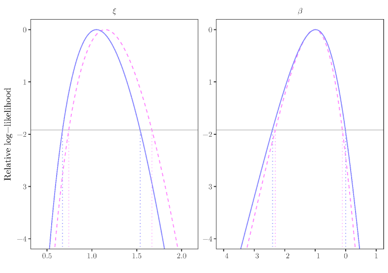
The study performed through the MCMPL does not produce the same significant results in support of the first treatment. The estimates are $\hat{\xi}_{M^{*}}=1.051$ (s.e. $0.221$) and $\hat{\beta}_{M^{*}}=-0.981$ (s.e. $0.564$), implying an hazard ratio equal to $e^{-\hat{\xi}_{M^{*}}\hat{\beta}_{M^{*}}}=2.806$. Testing $H_{0}\!:\beta=0$ by means of the MPL ratio statistic leads now to a more dubious conclusion, since the $p$-value equals 0.049, and such uncertainty is reflected by the 0.95 confidence interval for $\beta$ obtained by inversion of the same quantity, namely (-2.400, -0.004). A similar interval for $\xi$ is instead (0.672, 1.538). Figure 1 provides a graphical representation of the inferential discrepancy existing between the two contrasted methods, even in this case with a moderate value of $N$.

Inference on the relative risk can also be made by fitting a stratified Cox proportional hazards regression by means of the R function coxph, introduced in Section 5.4. Specifically, under this model the estimated risk ratio is equal to 1.953 (s.e. 1.054), with corresponding 0.95 confidence interval (0.641, 5.950) returned as output. The analogue Wald confidence regions for the Weibull relative risk based on the profile likelihood and MCMPL, resulting upon application of the Delta method, are instead (2.697, 3.702) and (2.378, 3.234), respectively. Thus, in this specific example, the interval obtained under the semiparametric Cox model is significantly wider than both those obtained assuming a Weibull distribution for the survival times, since there is a substantial price to be paid for the weaker assumption with such a moderate sample size.

Figure 1: Relative profile (dashed) and Monte Carlo modified profile (solid) log-likelihoods of the HIV data for $\xi$ and $\beta$, with corresponding 0.95 confidence intervals.

6 Discussion

This work shows how to exploit Monte Carlo simulation for widening the field of application of the MPL (Barndorff-Nielsen, 1980, 1983). Severini (1998) made a first step in this direction, yet his approximation is still not approachable enough to deal with the today’s degree of modelling sophistication for clustered units. Our solution, introduced in Section 3, helps to fill such a gap in accessibility and to solve the incidental parameters problem even when the experimental design imposes quite complex assumptions on the analysis. The suggested procedure is easy, implementable in broad generality and reasonably fast, and for these reasons could be thought of as the default choice in applications. Indeed, an extended version of the package panelMPL is currently under development and will also handle the automatic computation of the MCMPL for the model classes discussed here.

Section 4 addresses issues in inferences on the parameter of interest related to the presence of missing values in binary grouped data. In this case analytical calculation of Severini’s MPL is practicable but is not a simple task, while its approximation can be done by means of a simple two-step procedure to simulate the required Monte Carlo samples. Results of simulation studies are presented here for the logistic regression scenario and for the probit regression in the Supplementary material. In the analysis of MCAR observations Monte Carlo simulation is found unnecessary to compute the MPL, as the inferential precision of the MCAR MCMPL appears equivalent to that of the analytical MPL which disregards the missing data. Remarkably, the MNAR MCMPL sets an example of robustness to the ignorable incompleteness of the data. When the true mechanism of missingness is nonignorable, the MNAR MCMPL proves to be generally more accurate than Severini’s function, especially if $T$ is not too small, for any $N$. Justifications for this outcome are given in Section 4.3. To explore the usefulness of the Monte Carlo strategy when computing the MPL on partially MAR or partially missing always at random data for inference about $\psi$ (Little et al., 2017) could be another possible direction of research.

Clustered survival times subject to right-censoring are discussed in Section 5. Under the Weibull regression model with group-related intercepts, our proposed approximation to the MPL is made necessary by the lack of distributional assumptions on the random censoring mechanism. An explicit calculation of Severini’s modification requires full parametric specification of the density for the censoring times, whereas the Monte Carlo strategy enables to estimate it nonparametrically, using a conditional bootstrap (Davison and Hinkley, 1997, Algorithm 3.1). Experimental outcomes examined in Section 5.4 corroborate the theory pertaining to inference in the standard two-index asymptotic setting. Estimation of the parameter of interest via the MCMPL is preferable to that via the profile likelihood in every relevant respect and is not affected by the proportion of censored data in the sample. Finally, the computational burden demanded by existing alternative statistical procedures (Cortese and Sartori, 2016) is much heavier than that of the solution adopted here.

The potential room for future applications is vast, thanks to the generality of the methodology presented. One instance is given by semiparametric regression models where the incidental nuisance parameters are expressed as unknown real-valued functions (He and Severini, 2014).

References

- Agresti (2015) Agresti, A. (2015). Foundations of linear and generalized linear models. John Wiley & Sons.
- Baker (1995) Baker, S. G. (1995). Marginal regression for repeated binary data with outcome subject to non-ignorable non-response. Biometrics 51, 1042–1052.
- Barndorff-Nielsen (1980) Barndorff-Nielsen, O. E. (1980). Conditionality resolutions. Biometrika 67, 293–310.
- Barndorff-Nielsen (1983) Barndorff-Nielsen, O. E. (1983). On a formula for the distribution of the maximum likelihood estimator. Biometrika 70, 343–365.
- Bartolucci et al. (2016) Bartolucci, F., R. Bellio, A. Salvan, and N. Sartori (2016). Modified profile likelihood for fixed-effects panel data models. Econometric Reviews 35, 1271–1289.
- Bellio and Sartori (2003) Bellio, R. and N. Sartori (2003). Extending conditional likelihood in models for stratified binary data. Statistical Methods and Applications 12, 121–132.
- Bellio and Sartori (2006) Bellio, R. and N. Sartori (2006). Practical use of modified maximum likelihoods for stratified data. Biometrical journal 48, 876–886.
-
Bellio and
Sartori (2015)
Bellio, R. and N. Sartori (2015).
panelMPL: Modified profile likelihood estimation
for fixed-effects panel data models.
http://ruggerobellio.weebly.com/software.html. - Carey et al. (2015) Carey, V. J., T. Lumley, and B. Ripley. (2015). gee: Generalized Estimation Equation Solver. R package version 4.13-19.
- Carlin and Hodges (1999) Carlin, B. and J. Hodges (1999). Hierarchical proportional hazards regression models for highly stratified data. Biometrics 55, 1162–1170.
- Cortese and Sartori (2016) Cortese, G. and N. Sartori (2016). Integrated likelihoods in parametric survival models for highly clustered censored data. Lifetime Data Analysis 22, 382–404.
- Davison and Hinkley (1997) Davison, A. C. and D. V. Hinkley (1997). Bootstrap Methods and their Application. Cambridge University Press.
- De Bin et al. (2015) De Bin, R., N. Sartori, and T. Severini (2015). Integrated likelihoods in models with stratum nuisance parameters. Electronic Journal of Statistics 9, 1474–1491.
- Dempster et al. (1977) Dempster, A. P., N. M. Laird, and D. B. Rubin (1977). Maximum likelihood from incomplete data via the EM algorithm. Journal of the Royal Statistical Society. Series B (Methodological) 39, 1–38.
- Diciccio et al. (1996) Diciccio, T. J., M. A. Martin, S. E. Stern, and G. A. Young (1996). Information bias and adjusted profile likelihoods. Journal of the Royal Statistical Society. Series B (Methodological 58, 189–203.
- Fitzmaurice et al. (2008) Fitzmaurice, G., M. Davidian, G. Verbeke, and G. Molenberghs (2008). Longitudinal Data Analysis. Chapman & Hall/CRC.
- He and Severini (2014) He, H. and T. Severini (2014). Integrated likelihood inference in semiparametric regression models. METRON - International Journal of Statistics 72, 185–199.
- Ibrahim et al. (2001) Ibrahim, J. G., S. R. Lipsitz, and N. Horton (2001). Using auxiliary data for parameter estimation with non-ignorably missing outcomes. Journal of the Royal Statistical Society. Series C (Applied Statistics) 50, 361–373.
- Kenward and Molenberghs (1998) Kenward, M. G. and G. Molenberghs (1998). Likelihood based frequentist inference when data are missing at random. Statistical Science 13, 236–247.
- Lancaster (2000) Lancaster, T. (2000). The incidental parameter problem since 1948. Journal of Econometrics 95, 391–413.
- Lee and Nelder (2004) Lee, Y. and J. Nelder (2004). Conditional and Marginal Models: Another View. Statistical Science 19, 219–238.
- Liang and Zeger (1986) Liang, K.-Y. and S. L. Zeger (1986). Longitudinal data analysis using generalized linear models. Biometrika 73(1), 13–22.
- Little et al. (2017) Little, R. J., D. B. Rubin, and S. Z. Zangeneh (2017). Conditions for ignoring the missing-data mechanism in likelihood inferences for parameter subsets. Journal of the American Statistical Association 112, 314–320.
- Little and Rubin (2002) Little, R. J. A. and D. B. Rubin (2002). Statistical Analysis with Missing Data (2nd ed.). Wiley, New York.
- McCullagh and Tibshirani (1990) McCullagh, P. and R. Tibshirani (1990). A simple method for the adjustment of profile likelihoods. Journal of the Royal Statistical Society. Series B (Methodological) 52, 325–344.
- Molenberghs and Verbeke (2005) Molenberghs, G. and G. Verbeke (2005). Models for Discrete Longitudinal Data. Springer, New York.
- Nelder and Mead (1965) Nelder, J. A. and R. Mead (1965). A simplex method for function minimization. The Computer Journal 7, 308–313.
- Neyman and Scott (1948) Neyman, J. and E. Scott (1948, January). Consistent estimates based on partially consistent observations. Econometrica 16, 1–32.
- Pace and Salvan (1997) Pace, L. and A. Salvan (1997). Principles of Statistical Inference from a Neo-Fisherian Perspective. World Scientific Publishing, Singapore.
- Parzen et al. (2006) Parzen, M., S. R. Lipsitz, G. M. Fitzmaurice, J. G. Ibrahim, and A. Troxel (2006). Pseudo-likelihood methods for longitudinal binary data with non-ignorable missing responses and covariates. Statistics in Medicine 25, 2784–2796.
- Pierce and Bellio (2006) Pierce, D. A. and R. Bellio (2006). Effects of the reference set on frequentist inferences. Biometrika 93, 425–438.
- Pierce and Bellio (2015) Pierce, D. A. and R. Bellio (2015). Beyond first-order asymptotics for Cox regression. Bernoulli 21, 401–419.
- R Core Team (2017) R Core Team (2017). R: A Language and Environment for Statistical Computing. Vienna, Austria: R Foundation for Statistical Computing.
- Rubin (1976) Rubin, D. B. (1976). Inference and missing data. Biometrika 63, 581–592.
- Sartori (2003) Sartori, N. (2003). Modified profile likelihoods in models with stratum nuisance parameters. Biometrika 90, 533–549.
- Severini (1998) Severini, T. A. (1998). An approximation to the modified profile likelihood function. Biometrika 85, 403–411.
- Severini (2000) Severini, T. A. (2000). Likelihood Methods in Statistics. Oxford University Press.
- Severini (2007) Severini, T. A. (2007). Integrated likelihood functions for non-Bayesian inference. Biometrika 94, 529–542.
- Sinha et al. (2011) Sinha, S. K., A. B. Troxel, S. R. Lipsitz, D. Sinha, G. M. Fitzmaurice, G. Molenberghs, and J. G. Ibrahim (2011). A bivariate pseudolikelihood for incomplete longitudinal binary data with nonignorable nonmonotone missingness. Biometrics 67, 1119–1126.
- Therneau (2015) Therneau, T. M. (2015). survival: A Package for Survival Analysis in S. R package version 2.38.
- Troxel et al. (1998) Troxel, A. B., D. P. Harrington, and S. R. Lipsitz (1998). Analysis of longitudinal data with non-ignorable non-monotone missing values. Journal of the Royal Statistical Society. Series C (Applied Statistics) 47, 425–438.
- Troxel et al. (1998) Troxel, A. B., S. R. Lipsitz, and D. P. Harrington (1998). Marginal models for the analysis of longitudinal measurements with nonignorable non-monotone missing data. Biometrika 85, 661–672.