On the Discrepancy Between Two Zagreb Indices

Abstract.

We examine the quantity

$$S(G)=\sum_{uv\in E(G)}\min(\deg u,\deg v)$$

over sets of graphs with a fixed number of edges. The main result shows the maximum possible value of $S(G)$ is achieved by three different classes of constructions, depending on the distance between the number of edges and the nearest triangular number. Furthermore we determine the maximum possible value when the set of graphs is restricted to be bipartite, a forest, or to be planar given sufficiently many edges. The quantity $S(G)$ corresponds to the difference between two well studied indices, the irregularity of a graph and the sum of the squares of the degrees in a graph. These are known as the first and third Zagreb indices in the area of mathematical chemistry.

1. Introduction

1.1. The specialty of a graph

The following question appeared on the Team Selection Test for the 2018 United States International Math Olympiad team.

Problem 1

At a university dinner, there are 2017 mathematicians who each order two distinct entrées, with no two mathematicians ordering the same pair of entrées. The cost of each entrée is equal to the number of mathematicians who ordered it, and the university pays for each mathematician’s less expensive entrée (ties broken arbitrarily). Over all possible sets of orders, what is the maximum total amount the university could have paid?

This problem, posed by Evan Chen, proved extremely challenging for contestants, with only one full solution given on the contest. We can rephrase the question in more graph theoretic terms.

Definition 2.

Define the specialty of a graph $G$ to be

$$S(G)=\sum_{uv\in E(G)}\min(\deg u,\deg v)$$

where $E(G)$ is the edge set of a graph $G$.

The question posed to the contestants therefore is equivalent to evaluating

$$F(2017)=\max_{G\text{ has 2017 edges}}S(G).$$

The given solutions relied heavily on the fact that $2017=\binom{64}{2}+1$, and therefore the maximizing graph is near a complete graph. The purpose of this note is to determine

$$F(N)=\max_{G\text{ has $N$ edges}}S(G)$$

in general, as well as determine the maximum when $G$ is further restricted to be bipartite, a forest, or planar given sufficiently many edges in the final case.

1.2. Relation to Zagreb indices

The specialty of a graph is intimately related to two quantities of a graph, the irregularity of a graph and the sum of the squares of the degrees. First, Albertson [4] defines the irregularity of $G$, which we denote as $M_{3}(G)$, to be

$$M_{3}(G)=\sum_{uv\in E(G)}\left\lvert\deg u-\deg v\right\rvert.$$

Fath-Tabar [11] also defines this as the third Zagreb index, hence the choice of notation. Tavakoli and Gutman [20] as well as Abdo, Cohen, and Dimitrov [1] independently determined the maximum of $M_{3}(G)$ over all graphs with $n$ vertices.

On the other hand if the minimum of the degrees is replaced with a sum of the degrees in the definition of specialty, the corresponding quantity

$$M_{1}(G)=\sum_{uv\in E(G)}(\deg u+\deg v)=\sum_{v\in V(G)}(\deg v)^{2}$$

roughly counts the number of directed paths of length $2$ in $G$. The problem of maximizing this quantity over all graphs with a particular number of edges and vertices was a problem introduced in 1971 by Katz [15]. The first exact results in this problem were given by Ahlswede and Katona who in essence demonstrated that the maximum value is achieved on at least one of two possible graphs called the quasi-complete and quasi-star graphs [3]. However, as Erdős remarked in his review of the paper, “the solution is more difficult than one would expect” [9]. Ábrego, Fernández-Merchant, Neubauer, and Watkins furthered this result by determining the exact maximum in all cases [2]. However, given the complexity of the exact value of the upper bound, there was considerable interest in giving suitable upper bounds and a vast literature of such bounds developed. See [5], [6], [7], [8], [18], [18], [22], [21] for many results of this type. Many of these results stem from the area of mathematical chemistry and the above quantity is referred to as the first Zagreb index, $M_{1}(G)$. In this context, using the notation in [11], we resolve the problem of maximizing

$$S(G) =\frac{1}{2}\sum_{uv\in E(G)}(\deg u+\deg v-\left\lvert\deg u-\deg v\right\rvert)$$

$$=\frac{M_{1}(G)-M_{3}(G)}{2},$$

that is, the discrepancy between two of these already-studied graph invariants, over graphs with a fixed number of edges. Note that both $M_{1}(G)$ and $M_{3}(G)$ can both trivially have order of the square of the number of edges, and in this paper we in fact show that $S(G)$ has a strictly lower order. Furthermore, the maximum of $S(G)$ being of lower order extends to when $G$ is restricted to be a bipartite graph, a forest, or a planar graph. (The maximum value of $M_{1}(G)$ over a fixed number of edges is achieved by a star [3]. For $M_{3}(G)$ the maximum value over the set of all trees is achieved by a star [16] and one can easily check this extends to all planar graphs.)

1.3. Combinatorial interpretation

We end with an alternate combinatorial interpretation of $S(G)$ arising through the related $S^{\prime}(G)$ where

$$S^{\prime}(G)=\frac{1}{3}\sum_{uv\in E(G)}(\min(\deg u,\deg v)-1)=\frac{1}{3}S(G)-\#E(G).$$

Note that $S^{\prime}(G)$ provides a trivial upper bound for the number of triangles in a graph $G$ and a solution to the initial problem therefore provides an upper bound for the number of triangles in a graph with a specified number of edges.

Erdős gave a remarkably short proof that for graphs with $N=\binom{n}{2}+m$ edges (with $1\leq m\leq n$), the maximum number of triangles is achieved on a complete graph with $n$ vertices and an additional vertex connected to $m$ vertices in the clique [10]. The remarkable fact therefore is that the maximum of $S(G)$ is not always achieved on the same graphs as those that maximize the number of triangles, despite the optimal constructions agreeing for infinitely many integers (with a density of $\frac{2}{5}$).

2. Maximum Specialty over all Graphs

We will show the following result, which determines $F(N)$ in general.

Theorem 3.

Represent $N=\binom{n}{2}+m,1\leq m\leq n$ uniquely. Then the maximum value of $S(G)$ on a graph on $N$ edges is attained on a graph $G$ (which is not necessarily unique):

1. If $1\leq m\leq\frac{2n-3}{5}$, then $G$ is a clique of size $n$ and an additional vertex $v$ which connects to $m$ vertices in the clique. Then $F(N)=(n-1)\binom{n}{2}+\frac{m(3m-1)}{2}$ in this case.

2. If $\frac{2n-3}{5}\leq m\leq\frac{n-1}{2}$, then $G$ consists of three parts.

   • A clique of size $2m$ missing $m$ disjoint edges

   • A clique of size $n-2m$ with every vertex in this clique connected to every vertex in the previous “almost-clique”

   • A single vertex connected to every vertex in the “almost-clique” of size $2m$ but to no vertices in the clique of size $n-2m$

   In this case $F(N)=(n-1)\binom{n}{2}+m(4m-n+1)$.

3. If $\frac{n-1}{2}<m\leq n$, then $G$ is a ${K}_{n+1}$ missing $n-m$ disjoint edges in the clique. In this case $F(N)=n\binom{n}{2}+m(2m-n).$

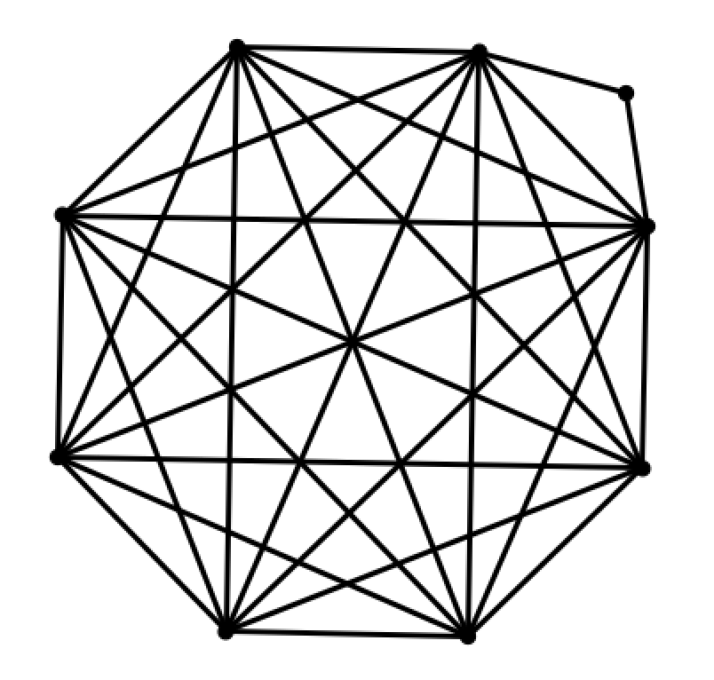
(a) $N=30$ edges

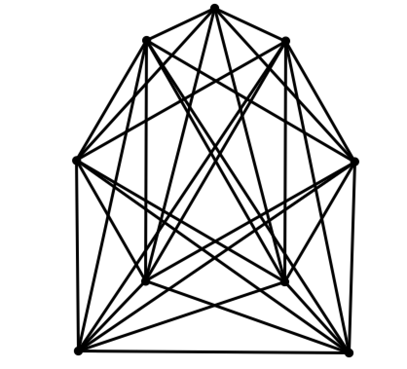
(b) $N=31$ edges

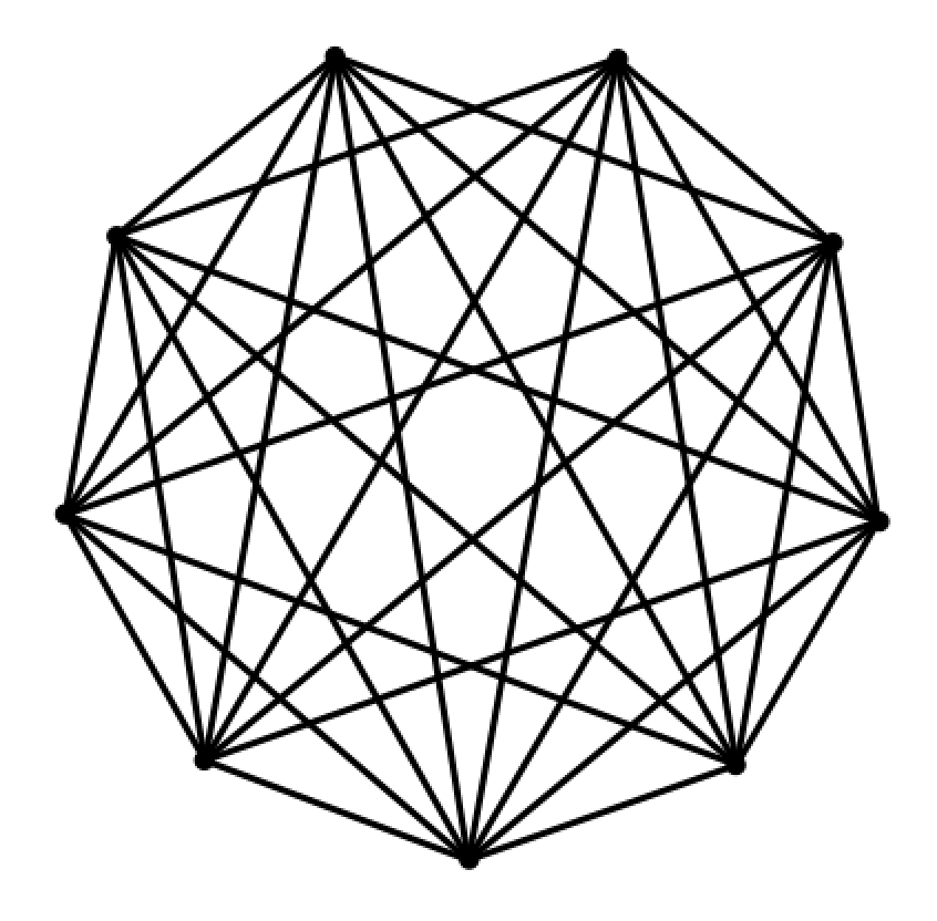
(c) $N=32$ edges

Figure 1. Maximal graphs in Theorem 3

There are two key aspects to the claimed maximal graph $G$. First, in each case $G$ has $n+1$ vertices. This is no coincidence, and is a key structural result in the course of proving Theorem 3. Secondly, these maximal graphs contain a “universal” vertex connected to all other vertices in both the first and third cases, but not in the second case. The analysis in the following sections is therefore often separated based on whether or not the graph contains such a “universal” vertex. As it turns out, in the case where the graph has no universal vertex and has $n+1$ vertices, we will show the construction in (ii) is optimal for all $1\leq m\leq\frac{n-1}{2}$.

Before proceeding with the bulk of the proof we need a series of definitions.

Definition 4.

In a graph $G$, define a vertex $v$ to be universal if $v$ connects to all other vertices in the graph $G$. Furthermore, let the set of graphs $G$ with a universal vertex be $\mathcal{UG}$.

Definition 5.

For an edge $uv\in E(G)$, define its weight to be $\min(\deg u,\deg v)$.

Definition 6.

Let

$$C(N)=\max_{\begin{subarray}{c}G\text{ has $N$ edges}\\ G\text{ has $n+1$ vertices}\\ G\notin\mathcal{UG}\end{subarray}}(S(G)).$$

We leave $C(N)$ undefined if no such graph $G$ exists.

For convenience we consider $N\leq 2$ separately. Note that $F(1)=2,F(2)=2$ as there is only one possible value in both cases. Since $1=\binom{1}{2}+1$ and $2=\binom{2}{2}+1$, these both agree with the claimed formula $n\binom{n}{2}+m(2m-n)$ in Theorem 3.

We now note that $C(N)$ is only defined if $1\leq m\leq\frac{n-1}{2}$.

Lemma 7.

If $m>\frac{n-1}{2}$ then every graph with $n+1$ vertices and $N$ edges is in $\mathcal{UG}$.

Proof.

We have $n+1$ vertices but $\binom{n}{2}+m=\binom{n+1}{2}-(n-m)$ edges. Since $2(n-m)<n+1$ and each edge can make at most $2$ vertices non-universal, there must be an universal vertex. ∎

Furthermore note that $F(N)$ is monotonically increasing as $N$ increases.

Lemma 8.

$F(N)$ is a strictly increasing function with respect to $N$.

Proof.

Consider graph $G$ with $S(G)=F(N)$. Make $G^{\prime}$ be $G$ with additional vertex $v$ connected to an arbitrary vertex in $G$. Then $F(N)=S(G)<S(G^{\prime})\leq F(N+1)$. ∎

The next observation was the key observation necessary for the original problem given to students on the Team Selection Test.

Lemma 9.

The maximum $F(N)$ is attained either on a graph with $n+1$ vertices or a graph with a universal vertex.

Proof.

Consider a graph $G$ with $n^{\prime}\geq n+2$ vertices and no universal vertex. Let $v$ be the vertex with minimal degree $\ell\leq n^{\prime}-2$ and suppose the neighbors of $v$ are $v_{1},\ldots,v_{\ell}$. Since there is no universal vertex in $G$, each of $v_{1},\ldots,v_{\ell}$ has a vertex $w_{1},\ldots,w_{\ell}$ with $w_{i}v_{i}$ not being an edge for each $1\leq i\leq\ell$.

Now delete all edges $vv_{i}$ in $G$ and replace these edges with $v_{i}w_{i}$ and delete the vertex $v$. Call this new multigraph $G^{\prime}$. Note that $G^{\prime}$ has $n^{\prime}-1$ vertices and that multiple edges may arise in $G^{\prime}$ if and only if $v_{i}=w_{j}$ and $w_{j}=v_{i}$. Construct $G^{\prime\prime}$ by taking any pair of double edges, deleting one of them, and adding any missing edge of $G^{\prime}$ in its place. This is always possible since $N=\binom{n}{2}+m\leq\binom{n+1}{2}\leq\binom{n^{\prime}-1}{2}$.

Note that $G^{\prime\prime}$ has $n^{\prime}-1$ vertices and $S(G^{\prime\prime})\geq S(G)$. The second observation follows as every vertex in $G^{\prime\prime}$ has degree at least as large as in $G$, while the $\ell$ edges deleted from $G$ have been replaced with $\ell$ new edges with increased or the same weights. Iterating this procedure, we eventually terminate since the vertex count decreases every time. Furthermore, we terminate at a graph that either has a universal vertex or has $n+1$ vertices, with at least as large specialty as before, which implies the result. ∎

Surprisingly, one can leverage this observation to reduce the search of graphs which maximize $F(N)$ to only those on $n+1$ vertices.

Lemma 10.

The maximum $F(N)$ is attained on a graph with $n+1$ vertices.

Proof.

We induct on $N$. The cases when $N=1$ or $N=2$ are trivial so let $N\geq 3$ for the remainder of the proof. Suppose that the result holds for all smaller $N$ and set $N=\binom{n}{2}+m,1\leq m\leq n$. Note that $n\geq 2$ as $N\geq 3$. Now suppose for the sake of contradiction that the maximum is not attained on a graph with $n+1$ vertices. Therefore by Lemma 9, we know that there exists a graph $G$ with a universal vertex satisfying $S(G)=F(N)$ but no such graph with $n+1$ vertices. Therefore $G$ has $n^{\prime}\geq n+2$ vertices and $G$ has a universal vertex $v$. Label the neighbors of $v$ as $v_{1},\ldots,v_{n^{\prime}-1}$. Furthermore, let vertex $v_{i}$ have degree $d_{i}$.

Consider deleting $v$ from $G$. The remaining graph, $G^{\prime}$, has $N-n^{\prime}+1$ edges and the remaining vertices have degree $1$ less in $G^{\prime}$ than in $G$. Therefore, each of the remaining $N-n^{\prime}+1$ edge weights decrease by $1$ when going from $S(G)$ to $S(G^{\prime})$. Furthermore, the $n^{\prime}-1$ edges $vv_{i}$ have weight $d_{i}$ in $G$. Therefore the total loss from removing these edges is

$$\sum_{i=1}^{n^{\prime}-1}d_{i}=2N-n^{\prime}+1.$$

Thus

$$S(G) =(2N-n^{\prime}+1)+(N-n^{\prime}+1)+S(G^{\prime})$$

$$\leq 3N-2n^{\prime}+2+F(N-n^{\prime}+1)$$

$$<3N-2n+F(N-n),$$

where we have used $n^{\prime}\geq n+2$ in the final inequality.

However, consider $G^{\prime\prime}$ with $N-n=\binom{n-1}{2}+(m-1)$ edges that has $S(G^{\prime\prime})=F(N-n)$. If $2\leq m\leq n$ then $1\leq m-1\leq n-1$ so by the inductive hypothesis $G^{\prime\prime}$ can be taken to have $n$ vertices. If $m=1$, then $N-n={n-2\choose 2}+(n-1)=\binom{n}{2}$ and by the inductive hypothesis $F(N)$ is maximized on a graph with $n-1$ vertices. In this case, add an empty vertex to obtain $G^{\prime\prime}$. Let the vertices of $G^{\prime\prime}$ be $v_{1},\ldots,v_{n}$ and let $v_{i}$ have degree $d_{i}$. Now add a universal vertex $v$ to $G^{\prime\prime}$ to form graph $G^{\circ}$ with $(N-n)+n=N$ edges. The weights of all edges in $G^{\prime\prime}$ increase by $1$ and inserted edges $vv_{i}$ have weight $d_{i}+1$. Therefore

$$S(G^{\circ}) =S(G^{\prime\prime})+(N-n)+n+2(N-n)$$

$$=S(G^{\prime\prime})+3N-2n$$

$$=F(N-n)+3N-2n,$$

and we have constructed a graph on $N$ edges with $S(G^{\circ})>S(G)=F(N)$, a contradiction! Thus the inductive step is complete and the result follows. ∎

With this structural result one can already deduce that the specialty of graphs with a triangular number of edges is maximized with a complete graph.

Corollary 11.

If $m=n$, then $F(N)=n{n+1\choose 2}$.

Proof.

Note that $N=\binom{n}{2}+n={n+1\choose 2}$ in this case and that the maximal value $F(N)$ is attained on a graph with $n+1$ vertices by Lemma 10. Therefore the complete graph $K_{n+1}$ is the only possibility and the result follows. ∎

Furthermore, we can now derive an inductive relationship between $F(N)$ and $C(N)$.

Lemma 12.

$F(N)=\max(F(N-n)+3N-2n,C(N))$

Proof.

By Lemma 10 we know $F(N)$ is realized on a graph $G$ with $n+1$ vertices. If $G$ has no universal vertex then $F(N)=C(N)$. Otherwise $G$ has $n+1$ vertices and a universal vertex. We show that any such graph has specialty at most $F(N-n)+3N-2n$, and furthermore that there is a construction to achieve this bound. We now prove that $F(N)\leq F(N-n)+3N-2n$ if the graph $G$ has a universal vertex $v$. Let $v$ have neighbors $v_{1},\ldots,v_{n}$ as $G$ and let vertex $v_{i}$ have degree $d_{i}$. The edges $vv_{i}$ have weight $d_{i}$, for a total of $2N-n$. If we construct $G^{\prime}$ by removing $v$ from $G$, every remaining edge has decreased in weight by $1$. Therefore we have

$$S(G^{\prime})=S(G)-(N-n)-(2N-n)=F(N)-3N+2n.$$

But by the definition of $F$, we have $S(G^{\prime})\leq F(N-n)$, since $G^{\prime}$ has $N-n$ edges. Therefore it follows in this case that

$$F(N)\leq F(N-n)+3N-2n.$$

This bound can be achieved by taking a graph on $n$ vertices and $N-n$ edges with specialty $F(N-n)$ and adding a vertex that connects to every other vertex. An isolated vertex need be first added in the case $m=1$. The analysis mimics the previous paragraph, and this is in essence the same as the construction in Lemma 10.

Therefore, since either the optimum $G$ with $n+1$ vertices has a universal vertex or not, $F(N)=\max(F(N-n)+3N-2n,C(N))$ is forced to hold and the result follows. ∎

Corollary 13.

If $m>\frac{n-1}{2}$ then $F(N)=F(N-n)+3N-2n$.

Proof.

Note that by Lemma 7, the quantity $C(N)$ is not well-defined in this range. The argument of Lemma 12 goes through without change except $G$ is forced to have a universal vertex in this case. ∎

The final structural result we use relies on the key idea of the proof of the Havel-Hakimi algorithm [12] [13], which controls possible degree sequences of a simple graph. (A degree sequence of a graph is the list of degrees of its vertices in some order.)

Lemma 14.

Consider a graph $G$ with a weakly decreasing degree sequence $(d_{1},\ldots,d_{k})$ satisfying $d_{1}=k-2$ and $k\geq 2$. Then there exists a graph $G^{\prime}$ such that $G^{\prime}$ has the same degree sequence as $G$, $S(G^{\prime})\geq S(G)$, and one vertex of degree $d_{1}$ in $G^{\prime}$ is connected to all vertices except a vertex of minimal degree.

Proof.

Label the vertices of $G$ as $v_{1},\ldots,v_{k}$ with the degree of $v_{i}$ being $d_{i}$. Now the neighborhood of $v_{1}$ is missing a unique vertex $v_{j}$. If $j=k$ then taking $G=G^{\prime}$ gives the result. Otherwise $j\neq k$ and note that $v_{j}$ has a neighborhood at least as large as $v_{k}$. Since $v_{1}$ is connected to $v_{k}$ but not $v_{j}$, there exists $v_{\ell}$ such that $(v_{\ell},v_{j})$ is an edge but $(v_{\ell},v_{k})$ is not. Then define $G^{\prime}$ by adding in $(v_{\ell},v_{k})$ and $(v_{1},v_{j})$ and removing $(v_{1},v_{k})$ and $(v_{\ell},v_{j})$. Note that $S(G^{\prime})-S(G)=d_{j}+d_{k}-d_{k}-\min(d_{\ell},d_{j})\geq 0$, and every vertex in $G^{\prime}$ has the same degree in $G$. The result follows. ∎

We now give the main technical lemma in this section of the paper. In particular we recursively bound the specialty of all graphs without a universal vertex.

Lemma 15.

Suppose that $N=\binom{n}{2}+m$ with $m<\frac{n-1}{2}$. Then it follows that $C(N)\leq\frac{(n-1)(3n-4)}{2}-m+C(N-(n-1))$.

Proof.

Note that $N-(n-1)=\binom{n-1}{2}+m$ and therefore since $n-2m>1$ it follows that $(n-1)-2m\geq 1$. Thus the right hand side of the claimed inequality is well defined. Now consider $G$ with $n+1$ vertices, no universal vertex, and such that $S(G)=C(N)$. Furthermore note that there is a vertex of degree $n-1$ as the average degree is $\geq\frac{n(n-1)}{n+1}>n-2$ and there is no universal vertex in $G$.

Now let $G$ have vertices $v_{1},\ldots,v_{n+1}$ with $\deg v_{i}=d_{i}$, and where $d_{i}$ is a nondecreasing sequence. By Lemma 14 we can further assume that in $G$, $v_{1}$ connects to $v_{2}$ through $v_{n}$ but not $v_{n+1}$. Furthermore, note that $d_{n+1}$ is not $n-1$ as otherwise $\sum_{i=1}^{n+1}d_{i}=(n+1)(n-1)=2\left(\binom{n}{2}+m\right)$ which implies $m=\frac{n-1}{2}$, a contradiction.

Suppose that $v_{n+1}$ is connected to $\ell$ vertices of degree $d_{n+1}$. Then we claim that

$$S(G)=(2N-(n-1)-d_{n+1})+(N-(n-1)-d_{n+1})+\ell+S(G^{\prime}),$$

where $G^{\prime}$ is induced subgraph of $G$ on $v_{2},\ldots,v_{n+1}$. This follows as

$$S(G) =\sum_{(v_{i},v_{j})\in E(G)}\min(d_{i},d_{j})$$

$$=\sum_{\begin{subarray}{c}(v_{i},v_{j})\in E(G)\\ i,j\neq n+1\end{subarray}}\min(d_{i},d_{j})+d_{n+1}^{2}$$

$$=\sum_{\begin{subarray}{c}(v_{i},v_{j})\in E(G)\\ i,j\neq 1,n+1\end{subarray}}\min(d_{i},d_{j})+\sum_{i\neq 1,{n+1}}d_{i}+d_{n+1}^{2}$$

$$=\sum_{\begin{subarray}{c}(v_{i},v_{j})\in E(G)\\ i,j\neq 1,n+1\end{subarray}}(\min(d_{i},d_{j})-1)+(d_{n+1}^{2}-\ell)$$

$$+(3N-2d_{n+1}-2(n-1))+\ell$$

$$=S(G^{\prime})+3N-2d_{n+1}-2(n-1)+\ell.$$

The last step follows due to a few facts about the removal of $v_{1}$. Every edge $(v_{i},v_{j})$ in $E(G^{\prime})$ for $i,j\neq 1,n+1$ is has weight $1$ less than it does in $G$. The edges attached to $v_{1}$ are all removed. The edges attached to $v_{n+1}$ are between a degree $d_{j}$ and $d_{n+1}$ vertex, which has weight $d_{n+1}$ in $G$. In $G^{\prime}$, the degrees are $d_{j}-1,d_{n+1}$. If $d_{j}>d_{n+1}$ the weight is still $d_{n+1}$ in $G^{\prime}$, but if $d_{j}=d_{n+1}$ then the weight has been decremented by $1$. This happens to precisely $\ell$ edges, by definition, hence the claimed equality.

As $d_{n+1}<n-1$ and the remaining vertices have decreased degree by $1$, it follows that $G^{\prime}$ does not have a universal vertex and we find $S(G^{\prime})\leq C(N-(n-1))$. Therefore it follows that $S(G)\leq C(N-(n-1))+3N-2d_{n+1}-2(n-1)+\ell$.

The key claim is now that $\ell-2d_{n+1}\leq-4m$. This yields

$$C(N) \leq(3N-4m-2(n-1))+C(N-(n-1))$$

$$=\frac{(n-1)(3n-4)}{2}-m+C(N-(n-1)),$$

as desired.

Now suppose that $\ell>2d_{n+1}-4m$. Since the sum of all degrees in $G$ is $n^{2}-n+2m$ and then $n^{2}-n+2m=\sum_{i=1}^{n+1}d_{i}\leq(n)(n-1)+d_{n+1}$, we conclude $d_{n+1}\geq 2m$. Further note from earlier that $d_{n+1}\leq n-2$. Therefore it follows that there are at least $\ell+1\geq 2d_{n+1}-4m+2$ vertices of degree $d_{n+1}$ and thus

$$n^{2}-n+2m=\sum_{i=1}^{n+1}d_{i} \leq d_{n+1}(2d_{n+1}-4m+2)$$

$$+(n-1)(n+1-(2d_{n+1}-4m+2)).$$

But note that the rightmost expression is a convex function in $d_{n+1}$. Thus, its maximum possible value over $d_{n+1}\in[2m,n-2]$ is attained at an endpoint. But its values at $d_{n+1}=2m$ and $d_{n+1}=n-2$ both equal $n^{2}-n+2m+(2m-n+1)$. Since $m<\frac{n-1}{2}$, this is strictly less than $n^{2}-n+2m$, a contradiction. ∎

Using this lemma we can now calculate $C(N)$ explicitly.

Lemma 16.

For $1\leq m\leq\frac{n-1}{2}$,

$$C(N)=(n-1)\binom{n}{2}+m(4m-n+1).$$

Proof.

The construction given in part (ii) of Theorem 3 is valid in the given range and has no universal vertex for any $1\leq m\leq\frac{n-1}{2}$ while achieving the claimed bound.

Now the key point is that when $m=\frac{n-1}{2}$ there is a single isomorphism class of graphs that we are maximizing over for $C(N)$, a $K_{n+1}$ missing a perfect matching. In this case every edge has weight $n-1$ and the result follows.

Otherwise, since $N=\binom{n}{2}+m$, applying Lemma 15 $n-2m-1$ times inductively yields

$$C(N)\leq\sum_{i=2m+2}^{n}\left(\frac{(i-1)(3i-4)}{2}-m\right)+C\left(\binom{2m+1}{2}+m\right)$$

$$=(n-1)\binom{n}{2}+m(4m-n+1)$$

since ${2m+1\choose 2}+m$ is precisely in the $m=\frac{n-1}{2}$ case already discussed. The result follows. ∎

Lemma 17.

We claim that

• If $1\leq m\leq\frac{2n-3}{5}$ then $F(N)\leq(n-1)\binom{n}{2}+\frac{m(3m-1)}{2}$.

• If $\frac{2n-3}{5}\leq m\leq\frac{n-1}{2}$ then $F(N)\leq(n-1)\binom{n}{2}+m(4m-n+1)$.

• If $\frac{n-1}{2}<m\leq n$ then $F(N)\leq n\binom{n}{2}+m(2m-n)$.

With Lemma 17 and the constructions given in Theorem 3 the main result follows.

Proof.

We prove this by induction on $N$. The result is trivial for $N=1$ and $N=2$. Furthermore $N=4$ and $N=5$ follow from a direct verification and $N=3,6$ follow from Lemma 11. Now suppose we have proved the claim for all $N<\binom{n}{2}+m$ and now consider $N=\binom{n}{2}+m$. Note that since $N\geq 7$ it follows that $n\geq 4$ in the remaining analysis. Furthermore note that $N-n=\binom{n-1}{2}+{m-1}$, which is used throughout in the below analysis. We now consider cases based on the relative size of $m$ and $n$.

Case 1: If $m=1$ then by Lemma 12 and Lemma 16 if follows that

$$F(N) =\max\bigg{(}F\bigg{(}\binom{n-1}{2}\bigg{)}+3N-2n,(n-1)\binom{n}{2}+(5-n)\bigg{)}$$

$$=\max\bigg{(}(n-2)\binom{n-1}{2}+3\binom{n}{2}+3-2n,(n-1)\binom{n}{2}+(5-n)\bigg{)}$$

$$=(n-1)\binom{n}{2}+1$$

where we used Lemma 11 in the second step and $n\geq 4$ in the final step.

Case 2: If $2\leq m\leq\frac{2n-3}{5}$ then by Lemma 12 and Lemma 16 we find

$$F(N)=\max\bigg{(}F\bigg{(}\binom{n-1}{2}+m-1\bigg{)}+3N-2m,(n-1)\binom{n}{2}+m(4m-n+1)\bigg{)}.$$

Since $1\leq m-1\leq\frac{2(n-1)-3}{5}$ it follows that

$$F(N-n)+3N-2n=(n-2)\binom{n-1}{2}+\frac{(m-1)(3m-5)}{2}+3N-2n$$

$$=(n-1)\binom{n}{2}+\frac{m(3m-1)}{2}$$

and note that if $m\leq\frac{2n-3}{5}$ then $\frac{m(3m-1)}{2}\geq m(4m-n+1)$. Therefore

$$F(N)=\max\bigg{(}(n-1)\binom{n}{2}+\frac{m(3m-1)}{2},(n-1)\binom{n}{2}+m(4m-n+1)\bigg{)}$$

$$=(n-1)\binom{n}{2}+\frac{m(3m-1)}{2},$$

as desired.

Case 3: If $\frac{2n-3}{5}<m\leq\frac{2n}{5}$ then note that $1\leq m-1\leq\frac{2(n-1)-3}{5}$. Then

$$F(N-n)+3N-2n=(n-2)\binom{n-1}{2}+\frac{(m-1)(3m-5)}{2}+3N-2n$$

$$=(n-1)\binom{n}{2}+\frac{m(3m-1)}{2}.$$

Since $m(4m-n+1)\geq\frac{m(3m-1)}{2}$ in this range Lemma 12 implies

$$F(N)=\max\bigg{(}(n-1)\binom{n}{2}+\frac{m(3m-1)}{2},(n-1)\binom{n}{2}+m(4m-n+1)\bigg{)}$$

$$=(n-1)\binom{n}{2}+m(4m-n+1),$$

as desired.

Case 4: If $\frac{2n}{5}<m\leq\frac{n-1}{2}$ then note that $\frac{2(n-1)-3}{5}\leq m-1\leq\frac{(n-1)-1}{2}$. Therefore we compute

$$F(N-n)+3N-2n=(n-2)\binom{n-1}{2}+(m-1)(4m-n-2)+3N-2n$$

$$=(n-1)\binom{n}{2}+m(4m-n-3)+n.$$

Since $m(4m-n+1)\geq m(4m-n-3)+n$ in this range it follows by Lemma 12 that

$$F(N)=\max\bigg{(}(n-1)\binom{n}{2}+m(4m-n-3)+n,(n-1)\binom{n}{2}+m(4m-n+1)\bigg{)}$$

$$=(n-1)\binom{n}{2}+m(4m-n+1),$$

as desired.

Case 5: If $\frac{n-1}{2}<m<\frac{n+1}{2}$ then it follows that $m=\frac{n}{2}$. Then note that $\frac{2(n-1)-3}{5}\leq m-1=\frac{(n-1)-1}{2}$ and $m-1\geq 1$. Therefore using Corollary 13 we obtain

$$F(N)=F(N-n)+3N-2n$$

$$=(n-1)\binom{n}{2}+m(4m-n-3)+n$$

$$=(n)\binom{n}{2}+m(2m-n),$$

where $m=\frac{n}{2}$ is used in the final step.

Case 6: If $\frac{n+1}{2}\leq m\leq n$ then note that $\frac{(n-1)}{2}\leq m-1\leq n-1$. Thus

$$F(N)=F(N-n)+3N-2n$$

$$=(n-1)\binom{n-1}{2}+(m-1)(2m-n-1)+3\binom{n}{2}+3m-2n$$

$$=n\binom{n}{2}+m(2m-n),$$

as claimed.

Hence the result follows in all cases by induction. ∎

3. Maximum Specialty over Bipartite Graphs

In this section we compute

$$F_{B}(N)=\max_{\begin{subarray}{c}G\text{ has $N$ edges}\\ G\text{ is bipartite}\end{subarray}}(S(G)).$$

In particular we prove the following theorem.

Theorem 18.

Suppose that $N=n^{2}+m$ for $1\leq m\leq 2n+1$, this decomposition is unique for $N\geq 1$. Then we have two cases based on size of $m$.

• If $1\leq m\leq n$ then $F_{B}(N)=n^{3}+m^{2}$. This is achieved by taking a $K_{n,n}$ and an additional vertex that connects to $m$ vertices on one side of the original bipartition.

• If $n+1\leq m\leq 2n+1$ then $F_{B}(N)=n^{3}+n^{2}+m(m-n)$. This is achieved by taking a $K_{n+1,n+1}$ and removing $2n+1-m$ disjoint edges.

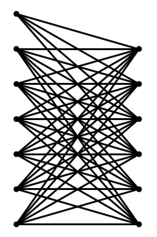
(a) $N=40$ edges

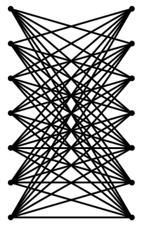
(b) $N=45$ edges

Figure 2. Maximal Graphs in Theorem 18

Note that $F_{B}(N)$ is trivially increasing; the proof is nearly identical to that of Lemma 8. This will be used throughout. The key to this section lies in an analog of Lemma 9, but in this case the proof gives a stronger conclusion. In a bipartite graph, a maximal vertex of one side of the bipartition is a vertex which connects to all the vertices in the other side.

Lemma 19.

For every integer $N$ there exists a graph $G$ with a bipartition $W$ and $X$ such that each partition has a maximal vertex and $S(G)=F_{B}(N)$.

Proof.

Suppose that $G$ has $N$ edges with $S(G)=F_{B}(N)$ but has at least one partition that does not have a vertex connected to all other vertices in the other partition. Let the bipartition of $G$ be $W$ and $X$, and suppose that $W=\{w_{1},\ldots,w_{k}\}$ and $X=\{x_{1},\ldots,x_{\ell}\}$. If $X$ does not have a universal vertex, then consider the vertex in $W$ of minimal degree, and without loss of generality let this be $w_{k}$. For each vertex $x_{i}$ adjacent to $w_{k}$ there exists an alternate vertex $w_{f(i)}$ in $W$ to which $x_{i}$ does not connect, by assumption. Replace the edges $w_{k}x_{i}$ with $w_{f(i)}x_{i}$, and remove $w_{k}$. Every remaining vertex has at least the same degree as it did before, and the replaced edges have at least the same weight. If $G^{\prime}$ is the altered graph, then $S(G^{\prime})\geq S(G)=F_{B}(N)$ and $G^{\prime}$ still has $N$ edges, hence $S(G^{\prime})=F_{B}(N)$. We can iterate this process, which decreases the vertex count each time. Thus it terminates, and it must terminate when both sides of the bipartition have a maximal vertex, as desired. ∎

With Lemma 19 it is now possible to derive two relations regarding $F_{B}(N)$.

Lemma 20.

If $N=n^{2}+m$ with $n+1\leq m\leq 2n+1$ then

$$F_{B}(N)\leq F_{B}(N-2n-1)+3(N-n)-2.$$

Otherwise $N=n^{2}+m$ with $1\leq m\leq n$ and

$$F_{B}(N)\leq\max\bigg{(}F_{B}(N-2n-1)+3(N-n)-2,F(N-2n)+2N+n(n-3)\bigg{)}.$$

Proof.

Consider a graph $G$ with bipartition $W=\{w_{1},\ldots,w_{k}\}$ and $X=\{x_{1},\ldots,x_{\ell}\}$ satisfying $k\geq\ell$. Furthermore define $w_{i}$ to have degree $y_{i}$ and $x_{j}$ to have degree $z_{j}$. Applying Lemma 19, we may assume that $y_{k}=\ell$ and $z_{\ell}=k$. Then consider $G^{\prime}$ when one removes $w_{k}$ and $x_{\ell}$. We find

$$F_{B}(N)=(S(G^{\prime})+N+1-k-\ell)+\sum_{j=2}^{\ell}\min(y_{j},\ell)+\sum_{j=2}^{k}\min(z_{j},k)+\ell.$$

If $\ell\geq n+1$ then $k+l\geq 2n+2$ so $G^{\prime}$ having $N+1-k-l$ edges implies

$$F_{B}(N) \leq S(G^{\prime})+N+1-k-\ell-2(N-\ell)+\ell$$

$$\leq F(N-2n-1)+3(N-n)-2.$$

Otherwise suppose that $n+1\leq m\leq 2n+1$ and $\ell\leq n$. Then we find $k+\ell\geq 2\sqrt{k\ell}\geq 2\sqrt{N}>2n+1$ so $k+\ell\geq 2n+2$ and

$$F_{B}(N) \leq(S(G^{\prime})+N+1-k-\ell)+\ell(\ell-1)+(N-\ell)+\ell$$

$$\leq F_{B}(N-2n-1)+2N-2n-1+n(n-1)$$

$$\leq F_{B}(N-2n-1)+3N-3n-2.$$

Finally, suppose that $1\leq m\leq n$ and $\ell\leq n$. Then $k+\ell\geq 2\sqrt{k\ell}\geq 2\sqrt{N}>2n$ so $k+\ell\geq 2n+1$ and we find

$$F_{B}(N) \leq(S(G^{\prime})+N+1-k-\ell)+\ell(\ell-1)+(N-\ell)+\ell$$

$$\leq F_{B}(N-2n)+2N+n(n-3),$$

as desired. ∎

We are now in a position to prove Theorem 18.

Lemma 21.

Let $N=n^{2}+m$ with $1\leq m\leq 2n+1$. Then we have two cases.

• If $1\leq m\leq n$ then $F_{B}(N)\leq n^{3}+m^{2}$.

• If $n+1\leq m\leq 2n+1$ then $F_{B}(N)\leq n^{3}+n^{2}+m(m-n).$

This gives Theorem 18 once one observes equality can be attained.

Proof.

The proof proceeds by a direct induction on $N$. Note that the result is trivial for $N=1$, $N=2$ and can easily be verified for $N=3$ and $N=4$. Therefore we will assume that we are considering $N\geq 5$ and therefore $n\geq 2$ in the below analysis.

Case 1: If $m=1$ then Lemma 20 gives that

$$F_{B}(N) \leq\max(F_{B}((n-1)^{2}-1)+3N-3n-2,F_{B}((n-1)^{2})+2N+n(n-3))$$

$$\leq\max(n^{3}-3n+5,n^{3}+1)=n^{3}+1,$$

as desired.

Case 2: If $m=2$ then Lemma 20 gives

$$F_{B}(N) \leq\max(F_{B}((n-1)^{2})+3N-3n-2,F_{B}((n-1)^{2}+1)+2N+n(n-3))$$

$$\leq\max(n^{3}+3,n^{3}+4)=n^{3}+4,$$

as desired.

Case 3: If $3\leq m\leq n$ then Lemma 20 gives

$$F_{B}(N) \leq\max(F_{B}((n-1)^{2}+m-2)+3(N-n)-2,F_{B}((n-1)^{2}+(m-1))+2N+n(n-3))$$

$$\leq\max(n^{3}+m^{2}-m+1,n^{3}+m^{2})=n^{3}+m^{2},$$

as desired.

Case 4: If $m=n+1$ then Lemma 20 gives

$$F_{B}(N) \leq F_{B}((n-1)^{2}+m-2)+3(N-n)-2$$

$$\leq n^{3}+m^{2}-m+1=n^{3}+n^{2}+m(m-n),$$

where $m=n+1$ is used in the final deduction.

Case 5: If $n+1<m\leq 2n+1$ then $m-2\geq(n-1)+1$ and Lemma 20 gives

$$F_{B}(N) \leq F_{B}((n-1)^{2}+m-2)+3(N-n)-2$$

$$\leq n^{3}+n^{2}+m^{2}-mn,$$

as desired.

Thus the inductive step follows in all cases and the proof is complete. ∎

4. Maximum Specialty over Forests and Planar Graphs

Unlike the previous sections, where the methods have been largely combinatorial, the key method for these two results is clever summation by parts. The algebraic casting of the problem was the key observation for the solution given by the contestant on the original Team Selection Test problem and the specific use of summation by parts also appears in Brendan McKay’s answer to [14] where specialty of planar graphs with a specific number of vertices rather than edges is maximized.

Theorem 22.

The maximum specialty over all forests with $N$ edges is $1$ if $N=1$ and $2N-2$ if $N\geq 2$.

Proof.

The case $N=1$ is clear, so let $N\geq 2$. A specialty of $2N-2$ is achieved with a path with $N$ edges.

Notice that given a forest, we can take two leaves in separate connected components and merge them. The resulting graph is still a forest, and the specialty has not decreased. Therefore, it suffices to study a graph $G$ that is a tree with $N$ edges and $N+1$ vertices.

Let $d_{1}\geq\cdots\geq d_{N+1}$ be the degrees of vertices $v_{1},\ldots,v_{N+1}$ of the graph $G$. Let $a_{i}$ for $1\leq i\leq N+1$ be the number of edges between $v_{i}$ and all $v_{j}$ with $j<i$. Using summation by parts we obtain

$$S(G)=\sum_{i=1}^{N+1}a_{i}d_{i}=\sum_{i=1}^{N+1}(d_{i}-d_{i+1})\bigg{(}\sum_{j=1}^{i}a_{j}\bigg{)},$$

where $d_{N+2}$ is defined to be $0$. Now each difference $d_{i}-d_{i+1}\geq 0$, and $\sum_{j=1}^{i}a_{j}$ is the number of edges in the induced subgraph of $G$ obtained by restricting to vertices $v_{1},\ldots,v_{i}$ only. Notice the corresponding subgraph has $i$ vertices and contains no cycles, so has at most $i-1$ edges. Therefore $\sum_{j=1}^{i}a_{j}\leq i-1$ for $1\leq i\leq N+1$. Then

$$S(G)\leq\sum_{i=1}^{N+1}(i-1)(d_{i}-d_{i+1})=\sum_{i=2}^{N+1}d_{i}=2N-d_{1}.$$

Since $N\geq 2$, and $G$ is a tree with $N$ edges, we know $d_{1}+\cdots+d_{N+1}=2N$, which implies the last equality. Furthermore, this gives $d_{1}\geq\frac{2N}{N+1}>1$ so $d_{1}\geq 2$. Therefore $S(G)\leq 2N-2$, and the result follows. ∎

For the planar case, first notice that the graphs that $S(G)$ on $N$ edges, without any restrictions, are planar for $N\leq 9$. Therefore it suffices to study $N\geq 10$. We now provide a inductive construction which provides the maximal specialty for $N\geq 33$.

Define $G_{N}$ as follows. First construct three vertices $v_{1},v_{2},v_{3}$ connected in a triangle and take $k=\left\lfloor\frac{N}{3}\right\rfloor+2$. In each successive stage, add $v_{i}$ where $v_{i}$ connects to $v_{i-1},v_{i-2},v_{i-3}$. Continue until we have $k$ vertices and $3k-6$ edges total. This is clearly planar, since each new vertex can be added on the outside of the planar embedding of the graph we are constructing. Now, if $N\equiv 1\pmod{3}$ add an additional vertex $v_{k+1}$ that connects only to $v_{k}$. If $N\equiv 2\pmod{3}$ add an additional vertex $v_{k+1}$ that connects to $v_{k},v_{k-1}$. When $k\geq 6$ the graph on $\{v_{1},\ldots,v_{k}\}$ has $k-6$ vertices of degree $6$, and two vertices of each degree $3,4,5$. Indeed, $\deg v_{1}=\deg v_{k}=3,\deg v_{2}=\deg v_{k-1}=4,\deg v_{3}=\deg v_{k-2}=5$, and the rest have degree $6$. It is easy to check that for $k\geq 9$ the weights $3,4,5$ are each assigned to $6$ edges and the remaining edges have weight $6$. Thus the specialty of the graph on $\{v_{1},\ldots,v_{k}\}$ with $N=3k-6$ edges is $6(N-18)+72=6N-36$. Furthermore, adding $v_{k+1}$ in the case when $N\equiv 1\pmod{3}$ adds a total of $4$ to the specialty, and adding $v_{k+1}$ in the $N\equiv 2\pmod{3}$ case adds a total of $10$ to the specialty. Therefore the total specialty is $6(N-1)-36+4=6N-38$ and $6(N-2)-36+10=6N-38$ in these cases. Hence our construction, which is valid when $k\geq 9$ or $N\geq 21$, yields

$$S(G_{N})=\bigg{\{}\begin{array}[]{lr}3N-36,&\text{if }N\equiv 0\pmod{3}\\ 6N-38,&\text{otherwise}.\end{array}$$

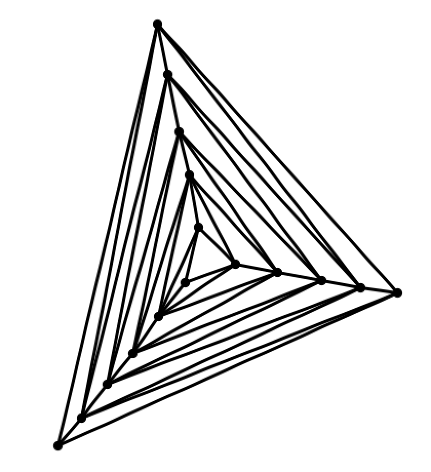
Figure 3. Maximal graph in Theorem 23 with $N=42$ edges

As we will see, this construction turns out to be optimal for the regime $N\geq 33$.

Theorem 23.

The maximum specialty over all planar graphs with $N\geq 33$ edges is $6N-36$ if $N\equiv 0\pmod{3}$ and $6N-38$ otherwise.

Proof.

The constructions are given above. Now recall the classical fact that any planar graph with $n\geq 3$ vertices has at most $3n-6$ edges. We can exploit this inequality in the same vein as in the proof of Theorem 22. Since $N\geq 33$ in this proof, the graphs we will consider always have at least $9$ vertices.

Let $v_{1},\ldots,v_{k}$ be the vertices of $G$ with $N$ edges, and suppose that $d_{1},\ldots,d_{k}$ are the respective degrees of the $v_{i}$ with $d_{1}\geq\cdots\geq d_{k}\geq 1$. Furthermore let $a_{i}$ for $1\leq i\leq k$ be the number of edges between $v_{i}$ and $v_{j}$ with $j<i$. Note that $\sum_{j=1}^{i}a_{j}$ is the number of edges in the induced subgraph of $G$ obtained by restricting to vertices $v_{1},\ldots,v_{i}$ only. Therefore $\sum_{j=1}^{i}a_{j}\leq 3i-6$ for $i\geq 3$ and $a_{1}=0,a_{1}+a_{2}\leq 1$. Furthermore, $\sum_{j=1}^{i}a_{j}\leq N$ for all $i$. Finally, for convenience let $d_{k+1}=0$. Then, as before,

$$S(G)=\sum_{i=1}^{k}a_{i}d_{i}=\sum_{i=1}^{k}(d_{i}-d_{i+1})\bigg{(}\sum_{j=1}^{i}a_{j}\bigg{)}.$$

We break into cases based on $N\pmod{3}$.

Case 1: $N\equiv 0\pmod{3}$, in which case we find

$$S(G) \leq(d_{2}-d_{3})+\sum_{i=3}^{k}(3i-6)(d_{i}-d_{i+1})$$

$$\leq d_{2}+2d_{3}+3\sum_{i=4}^{k}d_{i}$$

$$\leq 6N-3d_{1}-2d_{2}-d_{3},$$

using $\sum_{i=1}^{k}d_{i}=2N$.

Case 2: $N\equiv 1\pmod{3}$, in which case we find

$$S(G) \leq(d_{2}-d_{3})+\sum_{i=3}^{k-1}(3i-6)(d_{i}-d_{i+1})+(3k-8)(d_{k}-d_{k+1})$$

$$\leq d_{2}+2d_{3}+3\sum_{i=4}^{k-1}d_{i}+d_{k}$$

$$\leq 6N-3d_{1}-2d_{2}-d_{3}-2d_{k}$$

$$\leq 6N-3d_{1}-2d_{2}-d_{3}-2,$$

where we used the fact that $\sum_{i=1}^{k}a_{i}=N$ and $\sum_{i=1}^{k}a_{i}\leq 3k-6$ to deduce $\sum_{i=1}^{k}a_{i}\leq 3k-8$, based on the modular condition on $N$.

Case 3: $N\equiv 2\pmod{3}$, in which case we find

$$S(G) \leq(d_{2}-d_{3})+\sum_{i=3}^{k-1}(3i-6)(d_{i}-d_{i+1})+(3k-7)(d_{k}-d_{k+1})$$

$$\leq d_{2}+2d_{3}+3\sum_{i=4}^{k-1}d_{i}+2d_{k}$$

$$\leq 6N-3d_{1}-2d_{2}-d_{3}-d_{k}$$

$$\leq 6N-3d_{1}-2d_{2}-d_{3}-1,$$

where we used the fact that $\sum_{i=1}^{k}a_{i}=N$ and $\sum_{i=1}^{k}a_{i}\leq 3k-6$ to deduce $\sum_{i=1}^{k}a_{i}\leq 3k-7$, based on the modular condition on $N$. However, we can improve this bound by carefully considering the possible equality cases: we must have $d_{k}=a_{k}=1$, hence $N=\sum_{i=1}^{k}a_{i}=\sum_{i=1}^{k-1}a_{i}+1\leq 3(k-1)-6+1=3k-8$. Hence for any hypothetical equality cases $G$, we can sharpen to

$$S(G) \leq(d_{2}-d_{3})+\sum_{i=3}^{k-1}(3i-6)(d_{i}-d_{i+1})+(3k-8)(d_{k}-d_{k+1})$$

$$\leq d_{2}+2d_{3}+3\sum_{i=3}^{k-2}d_{i}+d_{k}$$

$$\leq 6N-3d_{1}-2d_{2}-d_{3}-2d_{k}$$

$$\leq 6N-3d_{1}-2d_{2}-d_{3}-2$$

and therefore there in fact are no equality cases, so that

$$S(G)\leq 6N-3d_{1}-2d_{2}-d_{3}-2$$

for all $G$ with $N$ edges and $N\equiv 2\pmod{3}$.

To finish note that if $G$ satisfies $3d_{1}+2d_{2}+d_{3}\geq 36$, then we are done regardless of which case we are in. Therefore it suffices to consider $3d_{1}+2d_{2}+d_{3}\leq 35$. Thus since $d_{3}\geq 1$ we have $5d_{2}\leq 3d_{1}+2d_{2}\leq 34$ and hence $d_{2}\leq 6$. Similarly since $6d_{3}\leq 3d_{1}+2d_{2}+d_{3}\leq 35$ it follows that $d_{3}\leq 5$, and thus $d_{i}\leq d_{3}\leq 5$ for $i\geq 3$. Now at most one edge has weight $d_{2}=6$, which is a potential edge between $v_{1},v_{2}$. The remaining edges all have at least one vertex of degree at most $5$, so

$$S(G)\leq 6+5(N-1)\leq 6N-38$$

and the result follows for $N\geq 39$. For $33\leq N\leq 38$ a more careful analysis involving $d_{k}$ is necessary. Clearly $d_{k}\leq 5$ since $G$ is planar, and we may assume we are working in the case where $3d_{1}+2d_{2}+d_{3}<36$. In particular, it is still true that at most one edge has weight $6$ and the rest have weight $\leq 5$. We can also assume the graph $G$ under consideration is a connected graph, since combining two vertices on the convex hulls of the embeddings of disconnected components $G_{1},G_{2}$ yields a graph that is connected and has at least the same specialty as before.

Case 1: Suppose that $2\leq d_{k}\leq 3$. If $d_{k}=2$ then note that

$$S(G)\leq 6+2(2)+5(N-3)=5N-5\leq 6N-38,$$

which follows as $N\geq 33$. Otherwise $d_{k}=3$ and

$$S(G)\leq 6+3(3)+5(N-4)=5N-5\leq 6N-38,$$

which follows as $N\geq 33$.

Case 2: Suppose that $d_{k}=4$. Then note that

$$S(G)\leq 6+4(4)+5(N-5)\leq 6N-36,$$

which holds for $N\geq 33$. Thus the result is settled for $N\equiv 0\pmod{3}$. If $N\equiv 1\pmod{3}$, then we derived earlier the inequality

$$S(G)\leq 6N-3d_{1}-2d_{2}-d_{3}-2d_{k}.$$

If $3d_{1}+2d_{2}+d_{3}+2d_{k}\geq 38$ then it is settled. Otherwise, $3d_{1}+2d_{2}+d_{3}+2d_{k}<38$. Note that $30=38-2d_{k}>3d_{1}+2d_{2}+d_{3}\geq 6d_{3}$ so $d_{3}<5$. Also, $5d_{2}\leq 3d_{1}+2d_{2}<30$ so $d_{2}\leq 5$. Thus that all edges except perhaps between $v_{1},v_{2}$ have weight $\leq 4$ and

$$S(G)\leq 4(N-1)+5<6N-38$$

for $N\geq 20$. Finally, if $N\equiv 2\pmod{3}$ then, similarly, we only need to handle the case when $3d_{1}+2d_{2}+d_{3}+d_{k}<38$. Then $6d_{3}<34$ or $d_{3}\leq 5$ and $30\geq 38-d_{3}-d_{k}>3d_{1}+2d_{2}\geq 5d_{2}$ so $d_{2}<6$. Therefore it follows that

$$S(G)\leq 5(N-4)+16\leq 6N-38,$$

which holds for $N=35$ and $N=38$, the cases under consideration.

Case 3: Suppose that $d_{k}=5$. If $N\equiv 1\pmod{3}$ then

$$S(G) \leq 6N-3d_{1}-2d_{2}-d_{3}-2d_{k}$$

$$\leq 6N-40<6N-38,$$

as desired. If $N\equiv 2\pmod{3}$ then

$$S(G)\leq 6N-3d_{1}-2d_{2}-d_{3}-d_{k},$$

so we only need consider the case $3d_{1}+2d_{2}+d_{3}+d_{k}<38$. That implies $3d_{1}<38-2d_{2}-d_{3}-d_{k}\leq 18$, hence $d_{1}=5$. Therefore the degree sequence is $(5,\ldots,5)$, implying $N\equiv 0\pmod{5}$ and thus $N=35$. Thus there are $14$ $5$’s in the degree sequence. However, by Theorem 1 in [19], no such planar graph exists. Finally, suppose $N\equiv 0\pmod{3}$. We need only consider cases when $3d_{1}+2d_{2}+d_{3}<36$. Thus $d_{3}<6$. Since $d_{3}\geq d_{k}=5$, we conclude $d_{3}=5$. Now if $d_{1}=d_{2}=5$ then $N=\equiv 0\pmod{5}$ but we are only considering $N=33$ and $N=36$ in this case. If $d_{1}=6$ and $d_{2}=5$ the degree sequence is $(6,5,\ldots,5)$, hence $N=33$ and there are $12$ $5$’s. However, no such planar graph exists by Theorem 2 in [19]. Finally, if $d_{1}=d_{2}=6$ then note that the degree sequence is $(6,6,5,\ldots,5)$, hence $N=36$ is forced and there are $12$ $5$’s. In this case $S(G)\leq 5(N-1)+6$, which is precisely $1$ more than the claimed bound of $6N-36$. For equality to occur, however, there must exist an edge between the two vertices of degree $6$. Removing this, we are left with a planar graph on $14$ vertices, each with degree $5$. However, this does not exist by Theorem 1 in [19]. Therefore this case is complete.

Case 4: Finally, suppose that $d_{k}=1$. If $N\equiv 0\pmod{3}$ then $S(G)\leq 6+1+5(N-2)$, which is at most the claimed bound of $6N-36$ when $N\geq 33$, as desired. If $N\equiv 2\pmod{3}$ then by the same reasoning above $S(G)\leq 6+5(N-2)+1$ and this is at most the claimed bound of $6N-38$ for $N\geq 35$, as desired. Finally if $N\equiv 1\pmod{3}$ then note that $S(G)\leq 1+6+5(N-2)$ as above and this is less than $6N-38$ for $N=37$ and exactly one more than the claimed bound for $N=34$. Consider $N=34$. In order to violate the claimed bound, equality must hold. In this case, we see $d_{k-1}\notin\{2,3,4\}$. In particular, in any of these cases there is an edge from $v_{k-1}$ not connected to $v_{k}$ and the above bound estimates that this edge has weight $5$ while it does not. If $d_{k-1}=1$ then $v_{k-1}$ and $v_{k}$ are forced to connect in the equality case. However, this creates a disconnected component in $G$, which we assumed was not the case. Thus $d_{k-1}\geq 5$. Remembering $3d_{1}+2d_{2}+d_{3}<36$, we have $d_{3}\leq 5$ and thus $d_{3}=\cdots=d_{k-1}=5$. Furthermore, for this equality to hold we need the edge of weight $6$ between $v_{1},v_{2}$. Thus $d_{2}=6$ and therefore since $3d_{1}+2d_{2}+d_{3}<36$ we find $3d_{1}<19$, implying $d_{1}=6$. Finally, $G$ has degree sequence $(6,6,5,\ldots,5,1)$ with $11$ $5$’s. For equality to occur we have an edge between the two vertices of degree $6$ and removing this vertex gives $(5,\ldots,5,1)$ where there are $13$ $5$’s. Removing the vertex of degree $1$ leaves a planar graph $(5,\ldots,5,4)$ with $12$ $5$’s. By Theorem 2 in [19], such a planar graph does not exist and we are finished. ∎

To see that the threshold above is sharp, notice that the icosahedral graph $I$ is planar, $5$-regular, has $N=30$ edges, and satisfies $S(I)=5\cdot 30>6\cdot 30-36$. Select arbitrary edge $uv$ of $I$ and add a new vertex attached only to $u,v$ to create planar graph $I^{\prime}$ with $N=32$ edges. Delete edge $uv$ from $I^{\prime}$ to create planar graph $I^{\prime\prime}$ with $N=31$ edges. Then $S(I^{\prime})=6\cdot 1+5\cdot 29+2\cdot 2>6\cdot 32-38$ and $S(I^{\prime\prime})=5\cdot 29+2\cdot 2>6\cdot 31-38$. Therefore, the result above does not hold for $N=30,31,32$. With little difficulty one can adapt the proof above to show that $I$ is optimal for $N=30$. Indeed, we have

$$S(G)\leq 6\cdot 30-3d_{1}-2d_{2}-d_{1}\leq 150$$

unless $3d_{1}+2d_{2}+d_{3}<30$, in which case $d_{2}\leq 5$ follows. Hence all edges have weight $\leq 5$, implying $S(G)\leq 5\cdot 30=150$. We suspect that similar arguments will yield that either $I^{\prime\prime}$ and $I^{\prime}$ or graphs with very similar degree sequences will be optimal for $N=31,32$, respectively.

We end by noting that, similar to a comment by Brendan McKay in [14], if a graph $G$ satisfies the property that every subgraph has average degree at most $\Delta$, then its specialty satisfies $S(G)\leq\Delta N$. The proof uses summation by parts in a identical manner to the above proofs. In particular, any graph family closed under minors, other than the set of all graphs, by [17], has linear specialty.

5. Open Questions

Given the results of Theorem 23, we immediately ask the following question.

Question 24

What is the maximum specialty of a planar graph when restricted to $N$ edges with $N$ between $10$ and $32$ but not equal to $30$ edges?

The results of this paper however otherwise settle the maximum specialty of a graph when restricted to a specific number of edges in the case of all graphs, bipartite graphs, forests, and planar graphs, and therefore it is natural to ask for finer control of specialty. In particular it is natural to ask which graphs maximize specialty with a fixed number of vertices and edges. However note that the optimizing graphs in Theorems 3, 18, 22, 23 always have the minimum possible number of vertices and therefore one can simply add on isolated vertices until the required vertex count. Therefore it is necessary for one to further restrict to the case where $G$ is connected. Let $\mathcal{CG}(N,n)$ be the set of connected graphs with $N$ edges and $n$ vertices.

Question 25

What is the behaviour of

$$F(N,n)=\max_{G\in\mathcal{CG}(N,n)}(S(G))?$$

In particular, how does the behaviour change when $N$ grows linearly in $n$ versus when $N$ grows quadratically in $n$? How does this behavior change when $G$ is further restricted to be bipartite?

6. Acknowledgements

The authors would like to thank Evan Chen for introducing them to the Question 1 and suggesting the associated general problem. The authors would also like Evan Chen and Colin Defant for reading the manuscript and providing helpful comments.

References

- [1] Hosam Abdo, Nathann Cohen, and Darko Dimitrov. Bounds and computation of irregularity of a graph. arXiv preprint arXiv:1207.4804, 2012.
- [2] Bernardo M Ábrego, Silvia Fernández-Merchant, Michael G Neubauer, and William Watkins. Sum of squares of degrees in a graph. Journal of Inequalities in Pure and Applied Mathematics, 10(64):369, 2009.
- [3] Rudolf Ahlswede and Gyula OH Katona. Graphs with maximal number of adjacent pairs of edges. Acta Mathematica Hungarica, 32(1-2):97–120, 1978.
- [4] Michael O Albertson. The irregularity of a graph. Ars Combinatoria, 46:219–225, 1997.
- [5] TC Edwin Cheng, Yonglin Guo, Shenggui Zhang, and Yongjun Du. Extreme values of the sum of squares of degrees of bipartite graphs. Discrete mathematics, 309(6):1557–1564, 2009.
- [6] Kinkar Ch Das. Maximizing the sum of the squares of the degrees of a graph. Discrete Mathematics, 285(1):57–66, 2004.
- [7] Kinkar Ch Das, Kexiang Xu, and Junki Nam. Zagreb indices of graphs. Frontiers of Mathematics in China, 10(3):567, 2015.
- [8] Dominique de Caen. An upper bound on the sum of squares of degrees in a graph. Discrete Mathematics, 185(1-3):245–248, 1998.
- [9] P. Erdős. Review of graphs with maximal number of adjacent pairs of edges. Math. Reviews 80g:05053.
- [10] Paul Erdős. On the number of complete subgraphs contained in certain graphs. Magyar Tud. Akad. Mat. Kutató Int. Közl, 7(3):459–464, 1962.
- [11] GH Fath-Tabar. Old and new zagreb indices of graphs. MATCH Commun. Math. Comput. Chem, 65:79–84, 2011.
- [12] S Louis Hakimi. On realizability of a set of integers as degrees of the vertices of a linear graph. i. Journal of the Society for Industrial and Applied Mathematics, 10(3):496–506, 1962.
- [13] Václav Havel. A remark on the existence of finite graphs. Casopis Pest. Mat., 80:477–480, 1955.
- [14] Brendan McKay (https://mathoverflow.net/users/9025/brendan mckay). A conjecture on planar graphs. MathOverflow. URL:https://mathoverflow.net/q/273694 (version: 2017-07-04).
- [15] Moshe Katz. Rearrangements of (0–1) matrices. Israel Journal of Mathematics, 9(1):53–72, 1971.
- [16] Jianxi Li, Yang Liu, and Wai Chee Shiu. The irregularity of two types of trees. Discrete Mathematics and Theoretical Computer Science, 17(3):203, 2016.
- [17] Wolfgang Mader. Homomorphieeigenschaften und mittlere kantendichte von graphen. Mathematische Annalen, 174(4):265–268, 1967.
- [18] Vladimir Nikiforov. The sum of the squares of degrees: Sharp asymptotics. Discrete Mathematics, 307(24):3187–3193, 2007.
- [19] EF Schmeichel and SL Hakimi. On planar graphical degree sequences. SIAM Journal on Applied Mathematics, 32(3):598–609, 1977.
- [20] Mostafa Tavakoli, Freydoon Rahbarnia, Madjid Mirzavaziri, Ali Reza Ashrafi, and Ivan Gutman. Extremely irregular graphs. Kragujevac Journal of Mathematics, 37(1):135–139, 2013.
- [21] Bo Zhou. Remarks on zagreb indices. MATCH Commun. Math. Comput. Chem, 57:591–596, 2007.
- [22] Bo Zhou and Dragan Stevanovic. A note on zagreb indices. MATCH Commun. Math. Comput. Chem, 56:571–578, 2006.