Pulse phase-resolved analysis of SMC X-3 during its 2016–2017 super-Eddington outburst

Abstract

The Be X-ray pulsar SMC X-3 underwent an extra long and ultraluminous giant outburst from 2016 August to 2017 March. The peak X-ray luminosity is up to $\sim 10^{39}$ erg/s, suggesting a mildly super-Eddington accretion onto the strongly magnetized neutron star. It therefore bridges the gap between the Galactic Be/X-ray binaries ($L_{\rm X}^{\rm peak}\leq 10^{38}$ erg/s) and the ultraluminous X-ray pulsars ($L_{\rm X}^{\rm peak}\geq 10^{40}$ erg/s) found in nearby galaxies. A number of observations were carried out to observe the outburst. In this paper, we perform a comprehensive phase-resolved analysis on the high quality data obtained with the Nustar and XMM-Newton, which were observed at a high and intermediate luminosity levels. In order to get a better understanding on the evolution of the whole extreme burst, we take the Swift results at the low luminosity state into account as well. At the early stage of outburst, the source shows a double-peak pulse profile, the second main peak approaches the first one and merges into the single peak at the low luminosity. The second main peak vanishes beyond 20 keV, and its radiation becomes much softer than that of the first main peak. The line widths of fluorescent iron line vary dramatically with phases, indicating a complicated geometry of accretion flows. In contrast to the case at low luminosity, the pulse fraction increases with the photon energy. The significant small pulse fraction detected below 1 keV can be interpreted as the existence of an additional thermal component located at far away from the central neutron star.

Keywords accretion, accretion disks — stars: neutron — pulsars: general — X-rays: binaries — X-rays: individual (SMC X-3)

1 Introduction

A Be/X-ray binary (BeXRB) consists of a Be star and a compact object. Only a few sources are identified as an accreting black-hole (e.g., MWC 656, Casares et al., 2014) or perhaps a white-dwarf (e.g., $\gamma$ Cassiopeia, Haberl et al., 1995; Postnov et al., 2017), while most of confirmed compact objects in BeXRBs are neutron stars (NSs; see Bildsten et al., 1997; Reig, 2011, for reviews), and half of these systems show X-ray pulsations (Haberl & Sturm, 2016). BeXRBs spend most time at the quiescence state, interrupted by quasi-periodic and less energetic outbursts or rare giant outbursts, i.e. type I and type II outbursts, respectively. A pulse phase-resolved analysis on the type II outburst is essential to test the accretion theory on strongly magnetized NSs at different accretion states.

The BeXRB SMC X-3 was discovered with the SAS-3 X-ray observatory in Small Magellanic Cloud (Clark et al., 1978), and its pulsation ($P=7.78$ s) was detected by other X-ray missions, e.g., Chandra (Edge et al, 2004), XMM-Newton (Haberl et al., 2008), and RXTE (Galache et al., 2008). From 2016 August to 2017 March, SMC X-3 underwent a super-Eddington outburst with a peak luminosity of $\sim 10^{39}$ erg/s, making it as the most luminous giant outburst reported in BeXRBs (Weng et al., 2016, 2017; Townsend et al., 2017; Tsygankov et al., 2017). Investigating the follow-up Swift monitoring observations, we found that the pulse profile exhibited a double-peak profile at the high luminosity state and then merging into the single peak at the low luminosity (Weng et al., 2017, hereafter Paper I). This evolution sequence is in agreement with an accretion scenario where the accretion column has a fan beam and a pencil beam pattern above and below the critical luminosity (Basko & Sunyaev, 1976; Becker et al., 2012; Mushtukov et al., 2015; Sartore et al., 2015), respectively. However, when taking a close look at the pulse profiles, we can find another narrow peak that follows the second main peak at the late stage of outburst, indicating the complicated geometry of NS magnetic field.

Investigating evolutions of isolated NSs spin period and its derivative, we could obtain the key informations of NSs magnetic field and characteristic age (e.g. Manchester & Taylor, 1977; Lyne & Graham-Smith, 2012; Gao et al., 2016, 2017). Alternatively, for BeXRBs, the observed NS spin frequency is modulated by the orbital motion, which allows measurement of the orbital parameters of the binary system (e.g., Li et al., 2011; Takagi et al., 2016). Townsend et al. (2017) tried to measure the evolution of the pulsar period, taking into account both the accretion induced spin-up effect (described by the Ghosh & Lamb relation; Ghosh & Lamb, 1979; Wang, 1981) and the modulation due to the binary orbital motion. In this way, assuming that the spin-up rate is proportional to $L_{\rm X}^{6/7}$, they tried to fit the orbital parameters; however, they could not obtain an adequate fit (i.e. the fitting residuals globally increase since MJD 57675, Figure 6 in their paper). Tsygankov et al. (2017) took the variation of bolometric correction into account, but the spin-up model still struggled to the data with the sharp and complex features shown in the fitting residuals (bottom panel of Figure 3 in their paper). Investigating the whole set of Swift monitoring data, we found that the spin-up rate and the 0.6–10 keV flux follows the power-law relation with an index of $0.84\pm 0.02$, which is in agreement with the predicted value of 6/7. But the relation deviates from the power-law at the peak and the low luminosity (Figure 5 in Paper I). Townsend et al. (2017) suggested that the variable accretion rate results in the complex changes in spin-up rate, which cannot be well described by the canonical spin-up model, and the higher order variations in the spin-up of SMC X-3 are requested. We utilized seven frequency derivatives to model the spin evolution and obtained the orbital parameters: the orbital period $P=44.52\pm 0.09$ days, the projected semi-major axis $asini=194\pm 1$ light seconds, the longitude of periastron $\omega=202\pm 2\arcdeg$ and an eccentricity of $e=0.259\pm 0.003$ (Weng et al. 2016, Paper I).

SMC X-3 was visited by Nustar at a high luminosity state during the 2016-2017 giant outburst rise (on 2016 August 13), one XMM-Newton (2016 October 14) and the second Nustar observations (2016 November 12) were subsequently carried out at the intermediate luminosity level during the decay of outburst (Table 1). The phase-averaged spectrum of XMM-Newton has been reported in Paper I, and the Nustar observations have been partially analyzed in Tsygankov et al. (2017). Since both XMM-Newton and Nustar have the large effective areas, high time resolution and moderate energy resolution, we present a detailed pulse phase-resolved analysis on these high quality data to explore the nature of accretion flows in this extreme outburst. We describe the data reduction in the next section and perform the timing and spectral analyses in Section 3. In order to describe the evolution of the whole burst, we also consider the Swift results presented in Paper I, in particular, at the low luminosity level. Discussion and conclusion follow in Section 4.

2 Data Reduction

The European Photon Imaging Camera (EPIC) is the main science instrument of XMM-Newton, and it is comprised of three X-ray CCD cameras, i.e. the pn and two MOS cameras. The time resolution is as good as 0.03 ms for the EPIC-pn timing mode data, and the energy resolution (FWHM) of EPIC is of $\sim 0.1-0.15$ keV at 6 keV . Because the EPIC-MOS observation was performed in imaging mode and seriously suffered from the pile-up effect, we only analyze the EPIC-pn data, which were taken in timing mode. The observation in the first 4.5 ks is contaminated by background flares, and therefore the data are excluded for the following analysis. The rest data with a net exposure time of 28 ks are reduced by using the Science Analysis System software (sas) version 16.0.0 with the standard filters: FLAG $=$ 0 and PATTERN $\leq$ 4. The source region is centered in RAWX = 38 with a width of 18 pixels, while the background region is centered in RAWX = 4 with a width of 2 pixels.

Table 1 : Log of observations

Obs Date	Observatory	ObsID	Net Exposure (ksec)	Period (s)	$L_{\rm X}$
2016 Aug 13	Nustar	90201035002	25	7.810645(1)	9.05$\pm$0.03
2016 Oct 14	XMM-Newton	0793182901	28	7.772007(3)	1.16$\pm$0.01
2016 Nov 12	Nustar	90201041002	42	7.771533(5)	1.62$\pm$0.01
Note:  $L_{\rm X}$: Phase-averaged unabsorbed X-ray luminosity in units of 1038 erg/s is calculated in 0.5–10 keV for XMM-Newton and 3–50 keV for Nustar data, assuming a distance to the source of 62.1 kpc (Hilditch et al., 2005; Graczyk et al., 2014; Scowcroft et al., 2016).

We extract the 0.3–12 keV source event and convert the observational time into the solar system barycenter time system with the task barycen. We subsequently adopt the epoch-folding method with the ftool efsearch to determine the spin frequency and its uncertainty by using a least squares fits of a Gaussian to the observed $\chi^{2}$ value versus the period (Leahy, 1987). The best fitted period is $7.772007\pm 0.000003$ s, and the consistent value can be obtained from the $Z_{1}^{2}$ test (Buccheri et al., 1983) as well. The light curves are generated in time bin size of 0.05 s, and are corrected for the telescope vignetting and point-spread-function losses with the sas task epiclccorr.

We create the spectral response files using the sas task rmfgen and arfgen for the subsequent phase-averaged and phase-resolved spectral analysis. The spectra are rebinned with the task specgroup to have at least 20 counts per bin and not to oversample the energy resolution of EPIC-pn by more than a factor of 3. The spectra are fitted in 0.5–10 keV with xspec 12.9.1 (Arnaud, 1996).

The Nustar observatory consists of two focusing instruments and two focal plane modules (FPMA and FPMB), has a time resolution better than 1 ms and an energy resolution of $\sim 0.3-0.4$ keV at 6 keV (Harrison et al., 2013). The Nustar data are processed with the packages and tools in heasoft version 6.21. The first Nustar observation was carried out at the peak of outburst; therefore, the source photons are extracted from a larger circular region with the radius of 120″. On the other hand, a smaller region with an aperture radius of 60″ is adopted for the second Nustar observation due to relatively low count rate. Meanwhile, the background photons are extracted from the source-free region. The source events in 3–50 keV are extracted and applied for the barycenter correction in order to calculate the spin period (Table 1). The spectra and light curves are produced with the proper corrections using the task nuproducts.

3 Results

3.1 Timing analysis

In order to investigate the energy-dependent pulse profiles, we extract the light curves in energy ranges of 0.3–1 keV, 1–2 keV, 2–3 keV, 3–5 keV, and 5–10 keV from XMM-Newton data, and in 3–5 keV, 5–10 keV, 10–20 keV, 20–30 keV, and 30–50 keV for Nustar data. Because the exposure time ($<1$ day) is much shorter than the orbital period, the binary orbital modulation in each observation is negligible, and the background-subtracted light curves are folded over the observed spin period with a phase bin number of 50. The evolution of pulse profiles is shown explicitly in Figure 1. At the high luminosity state, the typical fan beam pattern, i.e. the double-peak profile, is exhibited in the first Nustar observation. The two peaks have similar amplitudes and are separated by more than $\Delta\phi>0.4$. At the late stage, the two main peaks are converging ($\Delta\phi<0.3$), and the second peak disappears at the high energy ($>20$ keV, right panel of Figure 1). In addition, another narrow peak (hereafter, we call it “the minor peak”) emerges after the second peak.

The pulse fraction is calculated as $PF=(M-N)/(M+N)$, where $M$ and $N$ are the maximum and minimum count rates, respectively. The pulse fractions as a function of photon energy are plotted in Figure 2, in which the Nustar data points are in agreement with those shown in Figure 5 of Tsygankov et al. (2017). The NS spin modulation amplitude increases with the photon energy, while there is a hint of plateau in the range of 3-10 keV. The pulse fraction below 1 keV ($PF=0.218\pm 0.004$) is significantly lower than those detected beyond 1 keV.

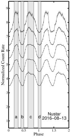
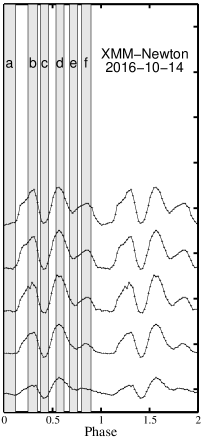
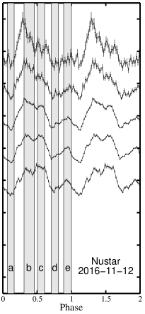
Fig. 1 : Energy-dependent pulse profiles. For Nustar data (left and right panels), from the bottom to the top, energy intervals correspond to 3–5 keV, 5–10 keV, 10–20 keV, 20–30 keV, and 30–50 keV, respectively. In the middle panel, we show the XMM-Newton pulse profiles in 0.3–1 keV, 1–2 keV, 2–3 keV, 3–5 keV, and 5–10 keV from the bottom to the top, respectively. We also arbitrarily shift up and plot two cycles of pulse profiles for clarity. The grey boxes mark the pulse phase regions in which the phase-resolved spectra are extracted and analyzed (Table 2).

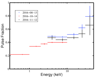
Fig. 2 : Evolution of energy-dependent pulse fraction.

3.2 Spectroscopy

3.2.1 Model

Following Paper I, we firstly employ the model consisting of a black-body (BB) plus a power-law component, and a Gaussian line (tbabs*(bbodyrad+powerlaw+gauss) in xspec) to fit the XMM-Newton data (Table 2). The phase-resolved spectral analysis is carried out to explore the X-ray properties of two main peaks, dips, and the minor peak if existed (the grey regions in Figure 1). There is no evidence for the change of absorption column density in different pulse phases; thus, we fix the value to $0.138\times 10^{22}$ cm^-2 in the following modelling (Table 2). The line width of iron emission changes dramatically with the pulse phase, and becomes too narrow to be resolved by XMM-Newton data in the phase range of $\sim 0.38-0.62$ (spectra c and d). In this case, we fix the line width to $\sigma=0.05$ keV.

Meanwhile, an absorbed exponentially cutoff power-law model with an additional fluorescent iron line is adopted for the Nustar spectral analysis. Due to the lack of sensitivity below 3 keV, the Nustar data cannot provide a substantial constraint on the neutral hydrogen column density. Thus, we fix the hydrogen column ($N_{\rm H}$) at $0.138\times 10^{22}$ cm^-2 derived from the XMM-Newton spectral fitting. In Tsygankov et al. (2017), an additional BB component with a temperature $\sim 0.8$ keV was included in the fitting to the first Nustar observation. However, this component was not detected in the simultaneous Swift/XRT observations (Paper I; Tsygankov et al., 2017; Townsend et al., 2017), which are much more sensitive below 3 keV. We do not know whether the thermal component detected by Nustar alone is real or due to the calibration uncertainty. Nerveless, the BB component only contributes less than 2% of total flux in 3–50 keV, and it does not affect the other parameters much. Therefore, we do not include this component in our work.

For the second Nustar observation, the iron line is marginally detected with a confidence level of $\sim 98\%$ according to $F$-test. In addition, since the width of the fluorescent iron line becomes narrower than the energy resolution of Nustar (Tsygankov et al., 2017), it was fixed at the value of 0.1 keV for the phase-averaged spectral analysis. But we do not involve the Gaussian line in the phase-resolved spectral fitting because of low significance level (Table 2).

3.2.2 Trends of Evolution

The first Nustar observation was carried out at the outburst rise with a high X-ray luminosity level. The significance of iron line in phase-resolved spectra is greater than 99.99% at least. The best-fit spectral parameters at two main peaks are almost the same with $\Gamma\sim 1.0$ and $E_{\rm cut}\sim 18$ keV. Alternatively, the radiation at two dips is harder, that is, $\Gamma\sim 0.9$ and $E_{\rm cut}\sim 12.5$ keV.

A cool thermal component ($kT_{\rm BB}\sim 0.2$ keV) is evidently shown in the XMM-Newton data obtained on 2016 October 14. The size of thermal component ($R_{\rm BB}\sim 220$ km without the color correction) is significantly larger than the radius of NS and varies with the pulse phases. The emission at the second main peak ($\Gamma=1.02$) is softer than the value ($\Gamma=0.93$) at the first peak. The fitted photon indices for two dips are $\Gamma=1.17$ and 0.93, respectively. The source has the hardest spectrum ($\Gamma=0.91$) at the minor peak. The significance of Gaussian line in phase-resolved spectra is greater than 96%.

Both the second Nustar and the XMM-Newton observations were performed during the decay of outburst, and they share the similar spectral evolution trend along the pulse phase. Compared with the XMM-Newton data, the second Nustar data have a lower luminosity and harder spectral profiles (Table 2). There is no significant correlation found among the best-fit parameters.

Table 2 : BEST-FIT SPECTRAL PARAMETERS

Phase	$N_{\rm H}$	$kT_{\rm BB}$	$R_{\rm BB}$	$\Gamma$	$E_{\rm cut}$	$E_{\rm Gau}$	$\sigma$	$f_{\rm X}$	$f_{\rm BB}/f_{\rm X}$	$\chi^{2}/$dof
	$10^{22}$ cm-2	keV	km		keV	keV	keV		$\%$
				2016 Aug 13	Nustar
0–1	$0.138^{{\dagger}}$	$\cdots$	$\cdots$	$1.00_{-0.01}^{+0.01}$	$16.4_{-0.2}^{+0.2}$	$6.38_{-0.06}^{+0.06}$	$0.34_{-0.07}^{+0.08}$	$1.95_{-0.01}^{+0.01}$	$\cdots$	1390.6/1291
a: 0.19–0.32	$0.138^{{\dagger}}$	$\cdots$	$\cdots$	$0.99_{-0.02}^{+0.02}$	$18.3_{-0.6}^{+0.6}$	$6.51_{-0.15}^{+0.16}$	$0.30_{-0.17}^{+0.24}$	$2.71_{-0.02}^{+0.02}$	$\cdots$	1136.1/1161
b: 0.41–0.51	$0.138^{{\dagger}}$	$\cdots$	$\cdots$	$0.90_{-0.04}^{+0.04}$	$12.6_{-0.6}^{+0.6}$	$6.38_{-0.09}^{+0.09}$	$0.19_{-0.10}^{+0.15}$	$0.95_{-0.01}^{+0.01}$	$\cdots$	741.7/749
c: 0.64–0.84	$0.138^{{\dagger}}$	$\cdots$	$\cdots$	$1.00_{-0.02}^{+0.02}$	$17.6_{-0.4}^{+0.5}$	$6.38_{-0.15}^{+0.17}$	$0.28_{-0.21}^{+0.19}$	$2.77_{-0.02}^{+0.02}$	$\cdots$	1336.6/1284
d: 0–0.08 & 0.98–1	$0.138^{{\dagger}}$	$\cdots$	$\cdots$	$0.91_{-0.04}^{+0.04}$	$12.4_{-0.6}^{+0.6}$	$6.38_{-0.12}^{+0.11}$	$0.27_{-0.12}^{+0.17}$	$0.90_{-0.01}^{+0.01}$	$\cdots$	736.4/733
				2016 Oct 14	XMM-Newton
0–1	$0.138_{-0.017}^{+0.018}$	$0.19_{-0.01}^{+0.01}$	$220.6_{-42.4}^{+49.4}$	$0.99_{-0.01}^{+0.01}$	$\cdots$	$6.63_{-0.10}^{+0.13}$	$0.34_{-0.10}^{+0.13}$	$0.25_{-0.01}^{+0.01}$	4.3	118.0/165
a: 0–0.12	$0.138^{{\dagger}}$	$0.18_{-0.01}^{+0.01}$	$234.3_{-18.3}^{+20.8}$	$1.17_{-0.03}^{+0.05}$	$\cdots$	$7.09_{-0.30}^{+0.46}$	$0.70_{-0.24}^{+0.70}$	$0.17_{-0.01}^{+0.01}$	5.5	172.3/156
b: 0.25–0.35	$0.138^{{\dagger}}$	$0.21_{-0.01}^{+0.01}$	$171.8_{-15.1}^{+17.5}$	$0.93_{-0.02}^{+0.02}$	$\cdots$	$6.63_{-0.14}^{+0.15}$	$0.26_{-0.17}^{+0.27}$	$0.32_{-0.01}^{+0.01}$	3.3	140.1/160
c: 0.38–0.46	$0.138^{{\dagger}}$	$0.17_{-0.01}^{+0.01}$	$252.9_{-21.6}^{+24.9}$	$1.03_{-0.02}^{+0.02}$	$\cdots$	$6.50_{-0.08}^{+0.09}$	$0.05^{{\dagger}}$	$0.18_{-0.01}^{+0.01}$	5.6	155.4/153
d: 0.54–0.62	$0.138^{{\dagger}}$	$0.18_{-0.01}^{+0.01}$	$211.1_{-27.0}^{+33.0}$	$1.02_{-0.02}^{+0.02}$	$\cdots$	$6.73_{-0.09}^{+0.09}$	$0.05^{{\dagger}}$	$0.36_{-0.01}^{+0.01}$	2.2	141.7/161
e: 0.68–0.76	$0.138^{{\dagger}}$	$0.19_{-0.01}^{+0.01}$	$247.1_{-18.1}^{+20.5}$	$0.97_{-0.02}^{+0.03}$	$\cdots$	$6.70_{-0.25}^{+0.30}$	$0.44_{-0.26}^{+0.41}$	$0.23_{-0.01}^{+0.01}$	5.8	129.5/153
f: 0.8–0.9	$0.138^{{\dagger}}$	$0.19_{-0.01}^{+0.01}$	$227.1_{-15.7}^{+17.5}$	$0.91_{-0.02}^{+0.03}$	$\cdots$	$6.76_{-0.55}^{+0.55}$	$0.78_{-0.52}^{+0.90}$	$0.27_{-0.01}^{+0.01}$	4.8	129.6/160
				2016 Nov 12	Nustar
0–1	$0.138^{{\dagger}}$	$\cdots$	$\cdots$	$0.66_{-0.02}^{+0.02}$	$14.9_{-0.3}^{+0.3}$	$6.41_{-0.11}^{+0.11}$	$0.1^{{\dagger}}$	$0.35_{-0.01}^{+0.01}$	$\cdots$	1152.8/1006
a: 0.07–0.17	$0.138^{{\dagger}}$	$\cdots$	$\cdots$	$0.69_{-0.07}^{+0.07}$	$16.3_{-1.5}^{+1.7}$	$\cdots$	$\cdots$	$0.21_{-0.01}^{+0.01}$	$\cdots$	502.4/532
b: 0.31–0.46	$0.138^{{\dagger}}$	$\cdots$	$\cdots$	$0.60_{-0.04}^{+0.04}$	$15.3_{-0.7}^{+0.7}$	$\cdots$	$\cdots$	$0.50_{-0.01}^{+0.01}$	$\cdots$	969.5/894
c: 0.51–0.61	$0.138^{{\dagger}}$	$\cdots$	$\cdots$	$0.72_{-0.05}^{+0.05}$	$13.7_{-0.8}^{+0.8}$	$\cdots$	$\cdots$	$0.43_{-0.01}^{+0.01}$	$\cdots$	798.1/729
d: 0.71–0.81	$0.138^{{\dagger}}$	$\cdots$	$\cdots$	$0.57_{-0.07}^{+0.07}$	$12.3_{-0.9}^{+1.0}$	$\cdots$	$\cdots$	$0.23_{-0.01}^{+0.01}$	$\cdots$	545.1/569
e: 0.89–1	$0.138^{{\dagger}}$	$\cdots$	$\cdots$	$0.57_{-0.05}^{+0.05}$	$11.8_{-0.7}^{+0.7}$	$\cdots$	$\cdots$	$0.30_{-0.01}^{+0.01}$	$\cdots$	699.8/670
Note:  $f_{\rm X}$: Unabsorbed X-ray flux in units of $10^{-9}$ erg cm-2 s-1 is calculated in 0.5–10 keV for XMM-Newton and 3–50 keV for Nustar data. $f_{\rm BB}/f_{\rm X}$: The percentage of total flux due to the thermal component. All errors are in the 90% confidence level. ${{\dagger}}$: The value of parameter is fixed.

4 Conclusions & Discussions

SMC X-3 experienced an extra long giant outburst, from 2016 August to 2017 March, with the peak X-ray luminosity of $\sim 10^{39}$ erg/s. A number of observations were carried out to observe the outburst, including one XMM-Newton and two Nustar observations (Weng et al., 2016, 2017; Townsend et al., 2017; Tsygankov et al., 2017). Thanks to the large effective area, the good time and energy resolution of XMM-Newton and Nustar, we perform a detailed phase-resolved analysis on these data to acquire more information on the extreme outburst of SMC X-3.

(1) At the early stage of outburst, SMC X-3 has a double-peak pulse profile in the broadband (3–50 keV), and the spectra at two main peaks are very similar. As the flux decays, the second main peak approaches the first one, and vanishes above 20 keV (Figure 1). That is, its spectrum becomes much softer than the spectrum at the first peak (Table 2). These results have been partially reported in Tsygankov et al. (2017) and Paper I.

(2) After the middle of 2016 October, a minor peak emerging after the second main peak was found in Paper I with the Swift monitoring data. Using the high quality data from XMM-Newton and Nustar, we confirm this feature, which however is not predicted in either the fan beam nor the pencil beam pattern (e.g., Bildsten et al., 1997). It might be due to the non-dipole component of NS magnetic field proposed by Tsygankov et al. (2017). We also find that the source has the hardest radiation at the minor peak.

(3) The first Nustar data taken at a high luminosity level exhibit larger pulse fraction than the second observation taken at the decay of outburst. For all three observations, we find that the pulse fraction increases with the photon energy. The significantly low pulse fraction at 0.3-1 keV can be interpreted as the existence of an additional thermal component located far away from the central NS, which was firstly detected in Paper I. Investigating a sample of bright X-ray pulsars, Hickox et al. (2004) suggested that the soft X-ray excess was a common feature in these systems. Here, the spectral fitting to the XMM-Newton data yields a ratio of the BB flux to the total flux $\sim 0.02-0.06$ (Table 2) and the size of BB component ($\sim 1000$ km with the color correction), which is a little bit smaller than the corotation radius of SMC X-3 ($\sim 6000$ km, see more details in Paper I). All these parameters are consistent with those of bright pulsars discussed in Hickox et al. (2004). For the pulsars with $L_{\rm X}\geq 10^{38}$ erg/s, the reasonable explanation for the soft X-ray excess is the reprocessing of hard X-rays by the inner region of truncated accretion disk (Hickox et al., 2004).

In contrast, the pulse fraction in the range of 0.5–2 keV starts to exceed that detected in 2-10 keV (Figure 1 in Paper I) when the pulse profile switches from the double-peak to the single-peak at low luminosity (Figure 4 in Paper I). That is, the pulse fraction has different correlations with the photon energy beyond and below the critical luminosity.

(4) The relatively large line widths ($\sigma\sim 0.34$ keV) shown in the first Nustar and XMM-Newton phase-averaged spectra could result from the Keplerian rotation at a radius of $\sim 1000$ km, which agrees with the size of cool thermal component (Paper I). Alternatively, the Gaussian line becomes narrower than the resolution of Nustar, and it can be explained in the way that the thermal component is pushed to a larger radius by the NS magnetosphere at lower luminosity (Lamb et al., 1973). In the XMM-Newton data fitting, the energy of iron line varies with the pulse-phase, suggesting different ionization stages (i.e. the He-like and the H-like ionization status) in different directions. Additionally, the small line widths ($<0.15$ keV), derived from the XMM-Newton data fitting in the phase range of $\sim 0.38-0.62$ (spectra c and d), indicate a complicated geometry of accretion column.

Acknowledgements  This research has made use of public data obtained from the High Energy Astrophysics Science Archive Research Center, provided by NASA’s Goddard Space Flight Center. We thank the anonymous referee for the helpful comments. We thank Jun-Xian Wang and Sergey Tsygankov for many valuable discussions. This work is supported by the National Natural Science Foundation of China under grants 11703014, 11673013, 11503027, 11373024, 11233003, 11433005, 11573023 and 11233001, National Program on Key Research and Development Project (Grant No. 2016YFA0400803 and 2017YFA0402703). H.H.Z. acknowledges support from the Natural Science Foundation from Jiangsu Province of China (Grant No. BK20171028), and the University Science Research Project of Jiangsu Province (17KJB160002). Q.R.Y. thanks support from the Special Research Fund for the Doctoral Program of Higher Education (grant No. 20133207110006).

References

- Arnaud (1996) Arnaud, K. A. 1996, in ASP Conf. Ser. 101, Astronomical Data Analysis Software and Systems V, ed. G. H. Jacoby &J. Barnes (San Francisco, CA: ASP), 17
- Basko & Sunyaev (1976) Basko, M. M., & Sunyaev, R. A. 1976, MNRAS, 175, 395
- Becker et al. (2012) Becker, P. A., Klochkov, D., Schönherr, G., et al. 2012, A&A , 544, A123
- Bildsten et al. (1997) Bildsten, L., Chakrabarty, D., Chiu, J., et al. 1997, ApJS, 113, 367
- Buccheri et al. (1983) Buccheri, R., Bennett, K., Bignami, G. F., et al. 1983, A&A, 128, 245
- Casares et al. (2014) Casares, J., Negueruela, I. Ribo, M. et al. 2014, Nature 505, 378
- Clark et al. (1978) Clark, G., Doxsey, R., Li F., Jernigan, J. G., & van Paradijs, J. 1978, ApJ, 221, L37
- Edge et al (2004) Edge, W. R. T., Coe, M. J., Corbet, R. H. D., Markwardt, C. B., & Laycock, S. 2004, Astron. Telegram, 225, 1
- Galache et al. (2008) Galache, J.L., Corbet, R.H.D., Coe, M.J., et al. 2008, ApJS, 177, 189
- Gao et al. (2016) Gao, Z.-F., Li, X.-D., Wang, N., et al. 2016, MNRAS, 456, 55
- Gao et al. (2017) Gao, Z.-F., Wang, N., Shan, H., et al. 2017, ApJ, 849, 19
- Ghosh & Lamb (1979) Ghosh, P., & Lamb, F. K. 1979, ApJ, 234, 296
- Graczyk et al. (2014) Graczyk, D., Pietrzyński, G., Thompson, I. B., et al. 2014, ApJ, 780, 59
- Haberl et al. (1995) Haberl F. 1995, A&A, 296, 685
- Haberl et al. (2008) Haberl F., Eger P., Pietsch W., 2008, A&A, 489, 327
- Haberl & Sturm (2016) Haberl, F., & Sturm, R. 2016, A&A , 586, A81
- Harrison et al. (2013) Harrison, F. A., Craig, W. W., Christensen, F. E., et al. 2013, ApJ, 770, 103
- Hickox et al. (2004) Hickox, R. C., Narayan, R., & Kallman, T. R. 2004, ApJ, 614, 881
- Hilditch et al. (2005) Hilditch, R. W., Howarth, I. D., & Harries, T. J. 2005, MNRAS, 357, 304
- Lamb et al. (1973) Lamb, F. K., Pethick, C. J., & Pines, D. 1973, ApJ, 184, 271
- Leahy (1987) Leahy, D. A. 1987, A&A, 180, 275
- Li et al. (2011) Li, J., Wang, W., & Zhao, Y. H. 2011, MNRAS, 423, 2854
- Lyne & Graham-Smith (2012) Lyne, A. G., & Graham-Smith, F. 2012, Pulsar Astronomy (4th ed.; Cambridge: Cambridge Univ. Press)
- Manchester & Taylor (1977) Manchester, R. N., & Taylor, J. H. (ed.) 1977, Pulsars (San Francisco, CA: Freeman)
- Mushtukov et al. (2015) Mushtukov, A. A., Suleimanov, V. F., Tsygankov, S. S., & Poutanen, J. 2015, MNRAS, 447, 1847
- Postnov et al. (2017) Postnov, K., Oskinova, L., & Torrejón, J. M. 2017, MNRAS, 465, L119
- Reig (2011) Reig, P., 2011, Ap&SS, 332, 1
- Sartore et al. (2015) Sartore, N., Jourdain, E., & Roques, J.-P. 2015, ApJ, 806, 193
- Scowcroft et al. (2016) Scowcroft, V., Freedman, W. L., Madore, B. F., et al. 2016, ApJ, 816, 49
- Takagi et al. (2016) Takagi, T., Mihara, T., Sugizaki, M., Makishima, K., & Morii M., 2016, PASJ, 68, S13
- Townsend et al. (2017) Townsend, L. J., Kennea, J. A., Coe, M. J., et al., 2017, MNRAS, 471, 3878
- Tsygankov et al. (2017) Tsygankov, S. S., Doroshenko, V., Lutovinov, A. A., Mushtukov, A. A., & Poutanen, J. 2017, A&A, 605, A39
- Wang (1981) Wang, Y.-M. 1981, A&A, 102, 36
- Weng et al. (2017) Weng, S.-S., Ge, M.-Y., Zhao, H.-H., Wang, W., Zhang, S.-N. 2017, Bian, W.-H., & Yuan, Q.-R. 2017, ApJ, 843, 69 (Paper I)
- Weng et al. (2016) Weng, S.-S., Ge, M.-Y., Zhao, H.-H., Wang, W., & Zhang, S.-N. 2016, Astron. Telegram, 9731, 1