Heuristics for Selecting Predicates for Partial Predicate Abstraction

Abstract

In this paper we consider the problem of configuring partial predicate abstraction that combines two techniques that have been effective in analyzing infinite-state systems: predicate abstraction and fixpoint approximations. A fundamental problem in partial predicate abstraction is deciding the variables to be abstracted and the predicates to be used. In this paper, we consider systems modeled using linear integer arithmetic and investigate an alternative approach to counter-example guided abstraction refinement. We devise two heuristics that search for predicates that are likely to be precise. The first heuristic performs the search on the problem instance to be verified. The other heuristic leverages verification results on the smaller instances of the problem. We report experimental results for CTL model checking and discuss advantages and disadvantages of each approach.
Keywords: predicate abstraction, widening, model checking

1 Introduction

Partial predicate abstraction [16] is a hybrid technique that combines advantages of predicate abstraction and fixpoint approximations for model checking infinite-state systems. It provides scalability by mapping part of the state space to a set of boolean variables representing a set of predicates on the mapped domain. It provides precision by representing the other part of the state space in its concrete domain and using approximation techniques to achieve convergence for computing the fixpoint. However, as in traditional predicate abstraction, a fundamental problem remains to be addressed: choosing the right set of predicates.

Counter-example guided abstraction refinement (CEGAR) addresses this fundamental problem in an incremental way. It basically expands the predicate set by discovering new predicates from the point where the spurious counter-example and the concrete behavior diverge. Craig interpolation [9] has been successfully used to automatically compute new predicates that would avoid the spurious counter-example. However, when the analysis continues with the new set of predicates new spurious behavior may be discovered and new predicates are generated and so on. Since model checking infinite-state systems is undecidable, the CEGAR loop may not terminate. Even if it terminates, it may end up generating a large set of predicates.

In this paper, we investigate an alternative approach to CEGAR for partial predicate abstraction. Since partial predicate abstraction is capable of representing some part of the state space in a concrete way, we need to identify how to partition the state space in terms of abstracting and approximating. We also would like to avoid two major problems with CEGAR: 1) choosing the initial set of predicates on variables that better be kept in their concrete domains and 2) ending up with a large set of predicates. We present two approaches to selecting predicates that would yield a precise and a feasible analysis. One approach measures the relative imprecision of the candidate predicates on the problem instance to be verified. Another approach uses a smaller instance of the problem and uses the verification results to infer a precise set of predicates to be used for verifying a larger instance.

Our heuristics are based on the properties of incremental abstraction that enables sound elimination of some of the candidates. We show that the elimination can be applied in both of the presented approaches. We have implemented both approaches using the Action Language Verifier (ALV) [19], which was also used to perform the verification experiments. For both approaches we present algorithms that select an optimal set of predicates based on the elimination heuristics and within the specified bound for the number of predicates. We use models on Airport Ground Traffic Control and a character-special device driver and perform measurements on various safety and liveness problem instances. Experimental results show effectiveness of the heuristics. We discuss the advantages and disadvantages of each approach.

The rest of the paper is organized as follows. Section 2 presents basic definitions and properties of partial predicate abstraction. Section 3 presents the two approaches to selecting the appropriate set of predicates. Section 4 presents experimental results. Section 5 discusses related work and Section 6 concludes with directions for future work.

2 Preliminaries

In this section we present preliminaries on the partial-predicate abstraction technique, which combines predicate abstraction and fixpoint approximations. We consider transition systems that are described in terms of boolean and unbounded integer variables.

Definition 1.

An infinite-state transition system is described by a Kripke structure $T=(S,I,R,V)$, where $S$, $I$, $R$, and $V$ denote the state space, set of initial states, the transition relation, and the set of state variables, respectively. $V=V_{bool}\cup V_{int}$ such that $S\subseteq\mathcal{B}^{|V_{bool}|}\times\mathcal{Z}^{|V_{int}|}$, $I\subseteq S$, and $R\subseteq S\times S$.

Definition 2.

Given a Kripke structure, $T=(S,I,R,V)$ and a set of states $A\subseteq S$, the pre-image operator, $pre[R](A)$, computes the set of states that can reach the states in $A$ in one step: $pre[R](A)=\{b\ |\ a\in A\ \wedge\ (b,a)\in R\}.$

$V$.	$s$, $t$, $a_{1}$, $a_{2}$, $z$: integer
	$pc1$, $pc2$: think, try, cr
$I$	$s=t\wedge pc_{1}=think\wedge pc_{2}=think$
Transitions:
$r^{try}_{i}$	$\equiv pc_{i}=think\wedge a_{i}^{\prime}=t\wedge t^{\prime}=t+1\wedge pc_{i}^{\prime}=try$
$r^{cr}_{i}$	$\equiv pc_{i}=try\wedge s\geq a_{i}\wedge z^{\prime}=z+1\wedge pc_{i}^{\prime}=cr$
$r^{think}_{i}$	$\equiv pc_{i}=cr\wedge s^{\prime}=s+1\wedge z^{\prime}=z-1\wedge pc_{i}^{\prime}=think$
$R$:	$\bigvee_{i=1,2}r^{try}_{i}\vee r^{cr}_{i}\vee r^{think}_{i}$

Figure 1: The ticket mutual exclusion algorithm for two processes. Variable $z$ is an addition to demonstrate the utilization of the proposed approach.

Abstract Model Checking and Predicate Abstraction

Definition 3.

Let $\varphi$ denote a set of predicates over integer variables. Let $\varphi_{i}$ denote a member of $\varphi$ and $b_{i}$ denote the fresh boolean variable that corresponds to $\varphi_{i}$. $\bar{\varphi}$ represents an ordered sequence (from index 1 to $|\varphi|$) of predicates in $\varphi$. The set of variables that appear in $\varphi$ is denoted by $V(\varphi)$. Let $\varphi^{\prime}$ denote the set of next state predicates obtained from $\varphi$ by replacing variables in each predicate $\varphi_{i}$ with their primed versions. Let $b$ denote the set of $b_{i}$ that corresponds to each $\varphi_{i}$. Let $V_{\sharp}=V_{\natural}\cup b\setminus V(\varphi)$.

Abstracting states

A concrete state $s^{\natural}$ is predicate abstracted using a mapping function $\alpha$ via a set of predicates $\varphi$ by introducing a predicate boolean variable $b_{i}$ that represents predicate $\varphi_{i}$ and existentially quantifying the concrete variables $V(\varphi)$ that appear in the predicates:

$$\alpha(s^{\natural})=\exists V(\varphi).(s^{\natural}\ \wedge\ \bigwedge^{|\varphi|}_{i=1}\varphi_{i}\iff b_{i}).$$ (1)

Concretization of abstract states

An abstract state $s^{\sharp}$ is mapped back to all the concrete states it represents by replacing each predicate boolean variable $b_{i}$ with the corresponding predicate $\varphi_{i}$:

$$\gamma(s^{\sharp})=s^{\sharp}[\bar{\varphi}/\bar{b}]$$ (2)

A concrete transition system can be conservatively approximated by an abstract transition system through a simulation relation or a surjective mapping function involving the respective state spaces in terms of existential abstraction.

Definition 4.

(Existential Abstraction) Given transition systems $T_{1}=(S_{1},I_{1},R_{1},V_{1})$ and $T_{2}=(S_{2},I_{2},R_{2},V_{2})$, $T_{2}$ approximates $T_{1}$ (denoted $T_{1}\sqsubseteq_{h}T_{2}$) iff

• $\exists s_{1}.(h(s_{1})=s_{2}\ \wedge\ s_{1}\in I_{1})$ implies $s_{2}\in I_{2}$,

• $\exists s_{1},s_{1}^{\prime}.(h(s_{1})=s_{2}\ \wedge\ h(s_{1}^{\prime})=s_{2}^{\prime}\ \wedge\ (s_{1},s_{1}^{\prime})\in R_{1})$ implies $(s_{2},s_{2}^{\prime})\in R_{2}$,

where $h$ is a surjective function from $S_{1}$ to $S_{2}$.

It is a known [14] fact that one can use a Galois connection $(\alpha,\gamma)$ to construct an approximate transition system. Basically, $\alpha$ is used as the mapping function and $\gamma$ is used to map properties of the approximate or abstracted system to the concrete system.

Theorem 1.

Assume $T_{1}\sqsubseteq_{\alpha}T_{2}$, $\phi$ denotes an ACTL formula that describes a property of $T_{2}$, $C(\phi)$ denotes the transformation of the correctness property by descending on the subformulas recursively and transforming every atomic formula $a$ with $\gamma(a)$ (see [7] for details), and $(\alpha,\gamma)$ forms a Galois connection and defines predicate abstraction and concretization as given in Equations 1 and 2, respectively. Then, $T_{2}\models\phi$ implies $T_{1}\models C(\phi)$ (see [16] for the proof).

For example, let $\phi$ be $AG(b_{1}\vee b_{2})$, where $b_{1}$ and $b_{2}$ represent $z=1$ and $z<1$, respectively, when the model in Figure 1 is predicate abstracted wrt to the set of predicates $\varphi=\{z=1,z<1\}$ and the Galois connection $(\alpha,\gamma)$ defined as in Equations 1 and 2. Then, $C(\phi)=AG(z\leq 1)$.

2.0.1 Computing A Partially Predicate Abstracted Transition System

We compute an abstraction of a given transition system via a set of predicates such that only the variables that appear in the predicates disappear, i.e., existentially quantified, and all the other variables are preserved in their concrete domains and in the exact semantics from the original system. As an example, using the set of predicates $\{z=1,z<1\}$, we can partially abstract the model in Figure 1 in a way that $z$ is removed from the model, two new boolean variables $b_{1}$ (for $z=1$) and $b_{2}$ (for $z<1$) are introduced, and $s$, $t$, $a_{1}$, $a_{2}$, $pc_{1}$, and $pc_{2}$ remain the same as in the original model.

Abstracting transitions

A concrete transition $r^{\natural}$ is predicate abstracted using a mapping function $\alpha^{\tau}$ via a set of current state predicates $\varphi$ and a set of next state predicates $\varphi^{\prime}$ by introducing a predicate boolean variable $b_{i}$ that represents predicate $\varphi_{i}$ in the current state and a predicate boolean variable $b_{i}^{\prime}$ that represents predicate $\varphi_{i}$ in the next state and existentially quantifying the current and next state concrete variables $V(\varphi)\cup V(\varphi^{\prime})$ that appear in the current state and next state predicates.

$$\alpha^{\tau}(r^{\natural})=\exists V(\varphi).\exists V(\varphi^{\prime}).(r^{\natural}\ \wedge\ CS\ \wedge\ \bigwedge^{|\varphi|}_{i=1}\varphi_{i}\iff b_{i}\wedge\ \bigwedge^{|\varphi|}_{i=1}\varphi_{i}^{\prime}\iff b_{i}^{\prime}),$$ (3)

where $CS$ represents a consistency constraint that if all the abstracted variables that appear in a predicate remains the same in the next state then the corresponding boolean variable is kept the same in the next state:

$$CS=\bigwedge_{\varphi_{i}\in\varphi}((\bigwedge_{v\in V(\varphi_{i})}v^{\prime}=v)\implies b_{i}^{\prime}\iff b_{i}).$$

As an example, for the predicate set $\{a>b,c=0\}$, $CS\equiv((a^{\prime}=a\wedge b^{\prime}=b\implies b_{1}^{\prime}=b_{1})\wedge(c^{\prime}=c\implies b_{2}^{\prime}=b_{2}))$, where $b_{1}$ represents predicate $a>b$ and $b_{2}$ represents predicate $c=0$.

For the model in Figure 1 and predicate set $\phi=\{z=1,z<1\}$, partial predicate abstraction of $r^{cr}_{i}$, $\alpha^{\tau}(r^{cr}_{i})$, is computed as $pc_{i}=try\ \wedge\ s\geq a_{i}\ \wedge\ ((b_{1}\wedge\neg b_{2}\wedge\neg b^{\prime}_{1}\wedge\neg b^{\prime}_{2})\vee\ (\neg b_{1}\wedge b_{2}\wedge(b^{\prime}_{1}\vee b^{\prime}_{2}))$ $\vee\ (\neg b_{1}\wedge\neg b_{2}\wedge\neg b^{\prime}_{1}\wedge\neg b^{\prime}_{2}))\ \wedge\ pc_{i}^{\prime}=cr.$

It is important to note that the concrete semantics pertaining to the integer variables $s$ and $a_{i}$ and the enumerated variable $pc_{i}$ are preserved in the partially abstract system.

The main merit of the combined approach is to combat the state explosion problem in the verification of problem instances for which predicate abstraction does not provide the necessary precision (even in the case of being embedded in a CEGAR loop) to achieve a conclusive result. As we have shown in [16], in such cases approximate fixpoint computations [19] may turn out to be more precise. The hybrid approach may provide both the necessary precision to achieve a conclusive result and an improved performance by predicate abstracting the variables that do not require fixpoint approximations.

2.1 Counter-example Guided Abstraction Refinement for Partial Abstraction

A common approach for dealing with imprecision in predicate abstraction is Counter-Example Guided Abstraction Refinement (CEGAR). The idea is to analyze the spurious counter-example path, identify the cause of divergence between the concrete behavior and the abstract path, and refine the system by extending the predicate set with refinement predicates. One of the challenges in CEGAR is controlling the size of the predicate set as new predicates get added. Since predicate abstracting a transition system is exponential in the number of predicates, if not controlled, CEGAR can easily blow up before providing any conclusive result.

We have implemented CEGAR for partial predicate abstraction for ACTL model checking (see [17] for details), which we will refer as CEGAAR in the rest of the paper. To deal with the predicate set size, we have used a breadth-first search (BFS) strategy to explore the predicate choices until a predicate set producing a conclusive result can be found. The algorithm keeps a queue of sets of predicates and in each iteration it removes a predicate set from the queue and computes the partial predicate abstraction with that predicate set. When a set of refinement predicates $rp$ is discovered for a given spurious counter-example path, rather than extending the current predicate set $\varphi$ with $rp$ in one shot, it considers as many extensions of $\varphi$ as $|rp|$ by extending $\varphi$ with a single predicate from $rp$ at a time and adds all these predicate sets to the queue to be explored using BFS. In the context of partial predicate abstraction, this strategy has been more effective in generating conclusive results compared to adding all refinement predicates at once.

3 Choosing the Predicates

In this section, we present two approaches to choosing predicates for partial predicate abstraction. Both approaches build on the concept of incremental abstraction and the guarantees provided by such abstractions that guide elimination of the candidate predicates. So, first we introduce the concepts related to incremental abstraction in Section 3.1 and present the individual approaches in sections 3.2 and 3.3.

3.1 Incremental Abstraction

Our goal is to assess imprecision of a set of predicates by building on the imprecision of the subsets, i.e., if at least one of the predicate sets $\varphi_{1}$ and $\varphi_{2}$ is not precise, we would like to be able to decide if combining the two sets, $\varphi_{1}\cup\varphi_{2}$, will incur at least the same level of imprecision or not. So we present some definitions below that will be used for imprecision assessment.

Definition 5 (Orthogonal abstractions).

Two abstraction functions $\alpha_{1}$ and $\alpha_{2}$ are orthogonal if $\alpha_{1}\circ\alpha_{2}=\alpha_{2}\circ\alpha_{1}$.

Definition 6 (Incremental abstraction).

An abstraction $\alpha$ is incremental if it can be built in terms of orthogonal abstractions $\alpha_{1}$ and $\alpha_{2}$, i.e., $\alpha=\alpha_{1}\circ\alpha_{2}=\alpha_{2}\circ\alpha_{1}$, and satisfy the property that for every concrete state $s$. $\alpha_{2}(s)\sqsubseteq\gamma_{1}(\alpha(s))$ and $\alpha_{1}(s)\sqsubseteq\gamma_{2}(\alpha(s))$.

Definition 7 (Disjoint abstractions).

Two predicate abstraction functions $\alpha_{1}$ and $\alpha_{2}$ are called disjoint if they are defined over predicates whose scopes are disjoint, i.e., $V(\varphi_{1})\cap V(\varphi_{2})=\emptyset$, where $(\varphi_{1},b_{1})$ and $(\varphi_{2},b_{2})$ denote the predicate sets and the boolean variables that define $\alpha_{1}$ and $\alpha_{2}$, respectively.

Predicate abstraction on disjoint predicate sets yield orthogonal abstractions, which can be used to construct incremental abstractions:

Lemma 1.

Given disjoint predicate abstraction functions $\alpha_{1}$ and $\alpha_{2}$ defined over $(\varphi_{1},b_{1})$ and $(\varphi_{2},b_{2})$, respectively, abstraction function $\alpha_{3}$ defined over $(\varphi_{1}\cup\varphi_{2},b_{1}\cup b_{2})$ can be defined incrementally.

Proof 1.

. i.e., $\alpha_{3}=\alpha_{2}\circ\alpha_{1}=\alpha_{1}\circ\alpha_{2}$ follows from the fact that $\alpha_{1}$ and $\alpha_{2}$ are disjoint:

$$\begin{split}&=\alpha_{2}\circ\alpha_{1}(s)\\ &=\exists V(\varphi_{2}).(\exists V(\varphi_{1}).s\wedge\bigwedge_{i=1}^{|\varphi_{1}|}\varphi_{1,}i\iff b_{1,i})\wedge\bigwedge_{i=1}^{|\varphi_{2}|}\varphi_{2,i}\iff b_{2,i}\\ &=\exists V(\varphi_{2}).(\exists V(\varphi_{1}).s\wedge\bigwedge_{i=1}^{|\varphi_{1}|}\varphi_{1,}i\iff b_{1,i}\wedge\bigwedge_{i=1}^{|\varphi_{2}|}\varphi_{2,i}\iff b_{2,i})\\ &=\exists V(\varphi_{2}).V(\varphi_{1}).(s\wedge\bigwedge_{i=1}^{|\varphi_{1}|}\varphi_{1,}i\iff b_{1,i}\wedge\bigwedge_{i=1}^{|\varphi_{2}|}\varphi_{2,i}\iff b_{2,i})\\ &=\alpha_{3}(s)\end{split}$$

Showing case $\alpha_{3}=\alpha_{1}\circ\alpha_{2}$ is similar. $\alpha_{1}(s)\sqsubseteq\gamma_{2}(\alpha_{3}(s))$ ($\alpha_{2}(s)\sqsubseteq\gamma_{1}(\alpha_{3}(s))$) also follows from the fact that $\alpha_{1}$ and $\alpha_{2}$ are disjoint and existential abstractions, and, hence, the new predicates on the new variables in $\alpha_{2}$ ($\alpha_{1}$) will introduce new behaviors as they were kept in their concrete domain when $\alpha_{1}$ ($\alpha_{2}$) was applied.

We would like to define a notion of imprecision that can be utilized in determining whether an abstraction may yield spurious behavior. The basic intuition in our formulation is that if an abstraction makes a transition to have a weaker precondition as to enable triggering more transitions or the same transitions but in additional ways in backward-image computation compared to what was possible in the concrete case then we consider that abstraction as imprecise. The formal definition follows.

Definition 8 (Transition-level Imprecision).

Let $T$ denote a transition system $T=(S,I,R)$ and $\alpha$ denote an abstraction function. $\alpha$ is imprecise wrt transitions $r_{1},r_{2}\in R$ if $r_{2}\wedge Range(Pre[r_{1}](true))\sqsubset\gamma(\alpha(r_{2})\wedge Range(Pre[\alpha(r_{1})](true)))$ or $r_{1}\wedge Range(Pre[r_{2}](true))\sqsubset\gamma(\alpha(r_{1})\wedge Range(Pre[\alpha(r_{2})](true)))$, where $Range(f)$ rewrites the formula $f$ by renaming variables with their next state versions.

Remark

It is important to note that Definition 8 points out to imprecision through the $\sqsubset$ operator, i.e., abstract version of transition $r_{2}$ is enabled from states that can be reached via executing the abstract version of $r_{1}$ in ways that were not possible in the concrete transition system $T$. An example is provided in Section 3.2.

The following lemma states that imprecise abstractions carry their imprecision in incremental abstractions.

Lemma 2.

Let $T$ denote a transition system $T=(S,I,R)$ and $\alpha_{1}$ and $\alpha_{2}$ denote disjoint abstraction functions. If $\alpha_{1}$ is imprecise wrt transitions $r_{1},r_{2}\in R$ then both $\alpha_{1}\circ\alpha_{2}$ and $\alpha_{2}\circ\alpha_{1}$ are imprecise wrt transitions $r_{1},r_{2}$.

Proof 2.

Follows from 1) Lemma 1, 2) predicate abstraction yielding an over-approximate pre-image operator, i.e., $Pre[\alpha_{1}(R)](true)\sqsubseteq\gamma(Pre[\alpha_{2}\circ\alpha_{1}(R)](true)])$, 3) monotonic nature of the pre-image computation, and 4) $a\sqsubset b$ and $b\sqsubseteq c$ implies $a\sqsubset c$.

Lemma 3 (Preservation for ECTL).

Given an existential abstraction function $\alpha$, an ECTL formula $\phi$, and transitions systems $T_{1}$ and $T_{2}$ such that $T_{1}\sqsubseteq_{\alpha}T_{2}$, $T_{1}\models\phi\implies T_{2}\models\alpha(\phi)$.

Proof 3.

Follows from the fact that existential abstraction defines a simulation relation between $T_{1}$ and $T_{2}$ and preserves transitions, and, hence, paths in the abstracted system.

Lemma 3 states that if a transition system satisfies an ECTL property then the existential abstraction of the abstracted transition system also satisfies this property.

Lemma 4.

Let $T$ denote a transition system $T=(S,I,R)$ and $\alpha_{1}$ and $\alpha_{2}$ denote orthogonal abstraction functions. If $\alpha_{1}(T)$ does not satisfy an ACTL property $\phi$ then neither $\alpha_{1}\circ\alpha_{2}(T)$ nor $\alpha_{2}\circ\alpha_{1}(T)$ satisfy $\phi$.

Proof 4.

Follows from the fact that existential abstraction preserves transitions between mapped states and, hence, preserves paths. If an ACTL property is not satisfied by $\alpha_{1}(T)$ then it satisfies the negation, which is an ECTL property. From Lemma 3 it follows that both $\alpha_{1}\circ\alpha_{2}(T)$ and $\alpha_{2}\circ\alpha_{1}(T)$ will contain the infeasible counter-example path.

Lemma 4 implies that if we are aware of an abstraction $\alpha$ that is imprecise for analyzing a transition system $T$ for a given ACTL property $\phi$, i.e., the property is not satisfied and the counter-example is infeasible, incremental abstractions that involve $\alpha$ will also be imprecise for verifying $\phi$.

3.2 Inferring Predicates from Transition-Level Imprecision

In this section, we present our first approach to choosing predicates, which is based on transition-level imprecision of predicates and builds upon Lemma 2. We compute imprecision of predicates wrt transition pairs for each predicate as well as for each pairwise combination of the predicates using algorithm CompTransLevelImp that is given in Figure 5. We quantify imprecision in terms of the number of additional predicate regions covered in enabling another transition for backward-image computation. When the imprecision is computed for an individual predicate (lines 8-17) the imprecision per transition pair can be 2 at maximum and when it is computed for a pair of predicates (lines 18-28) the same metric can be 4 at maximum. It should be noted that imprecision values for each pair of transition is summed up to compute the actual precision score for individuals (line 16) as well as for pairs of predicates (line 26).

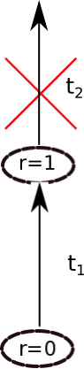
Figure 2: Concrete transition $t_{2}$ cannot be executed from a state that is reached via $t_{1}$.

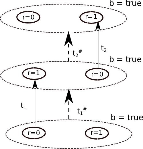
Figure 3: Abstracting $t_{1}$ and $t_{2}$ with respect to predicate set $\{r\leq 1\}$.

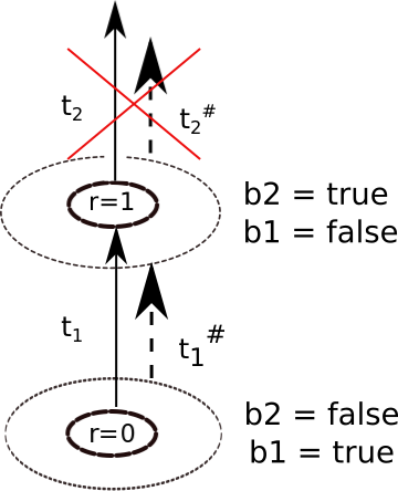
Figure 4: Abstracting $t_{1}$ and $t_{2}$ with respect to predicate set $\{r=0,r=1\}$.

As an example, consider the following transitions: $t_{1}\equiv pc_{1}=a\wedge r=0\wedge r^{\prime}=r+1\wedge pc_{1}^{\prime}=c$ and $t_{2}\equiv pc_{2}=a\wedge r=0\wedge r^{\prime}=r+1\wedge pc_{2}^{\prime}=c$. In the concrete semantics, $t_{1}\wedge Range(pre[t_{2}](true))$ yields false as illustrated in Figure 2 as there is no state from which we can execute $t_{1}$ and then $t_{2}$. If we use predicate abstraction while using the predicate set $\{r\leq 1\}$ and boolean variable $b$, we get the following abstract versions: $\alpha(t_{1})\equiv pc_{1}=a\wedge b\wedge b^{\prime}\wedge pc_{1}^{\prime}=c$ and $\alpha(t_{2})\equiv pc_{2}=a\wedge b\wedge b^{\prime}\wedge pc_{2}^{\prime}=c$. Now, if we compute $\alpha(t_{1})\wedge Range((pre[\alpha(t_{2})](true))$, the result will not be false as it evaluates to $pc_{1}=a\wedge b\wedge b^{\prime}\wedge pc^{\prime}_{2}=a\wedge b^{\prime}$. As shown in Figure 3, this means that abstract transition $t^{\sharp}_{2}$ is enabled from a state that is reached executing abstract transition $t^{\sharp}_{1}$. The way we quantify this extra behavior introduced by the abstraction is the number of extra predicate regions or cubes that enables the triggering of $t_{1}$ by $t_{2}$ when computing the image backward. In this case the additional region covered when triggering $t_{1}$ by $t_{2}$ is when the predicate evaluates to true, e.g, $r\leq 1$ or $b=true$. So the score for imprecision is 1 in this case. Figure 4 shows a case in which the predicate set $\{r=0,r=1\}$ avoids the imprecision that was possible with predicate set $\{r\leq 1\}$. This is because concrete state $r=0$ and concrete state $r=1$ are mapped to separate abstract states.

1:CompTransLevelImp($T=(S,I,R)$: Transition System,$\varphi$: Set of predicates)

2:Output: $IS:\varphi\to\mathcal{Z}$: Individual Imprecision Scores, $PwS:\varphi\times\varphi\to\mathcal{Z}$: Pairwise Imprecision Scores

3:$IS\leftarrow\lambda x.0$

4:$PwS\leftarrow\lambda x.y.0$

5:for each $r_{j}\in R$ do

6:     for each $r_{k}\in R$ do

7:         for each $\varphi_{i}\in\varphi$ do

8:              Let $\alpha_{i}$ pred. abs. using $(\{\varphi_{i},\},\{b_{i}\})$

9:              Let $Cube_{conc}$ denote the set $\{\varphi_{i},\neg\varphi_{i}\}$

10:              $conc\leftarrow r_{k}\wedge Range((pre[r_{j}](true)))$

11:              $concCov\leftarrow|\{cube|cube\in Cube_{conc}\text{ and }conc\wedge cube\not=false\}|$

12:              if $concCov<2$ then

13:                  $abs\leftarrow\alpha_{i}(r_{k})\wedge Range((pre[\alpha_{i}(r_{j})](true))$

14:                  Let $Cube_{abs}$ denote the set $\{b_{i},\neg b_{i}\}$

15:                  $absCov\leftarrow|\{cube|cube\in Cube_{abs}\text{ and }abs\wedge cube\not=false\}$

16:                  $IS\leftarrow IS[\varphi_{i}\mapsto IS[\varphi_{i}]+absCov-concCov]$

17:              end if

18:              for each $\varphi_{m}\in\varphi,\varphi_{m}\not=\varphi_{i}$ do

19:                  Let $\alpha_{c}$ pred. abs. using $(\{\varphi_{i},\varphi_{m}\},\{b_{i},b_{m}\})$

20:                  Let $Cube_{conc}$ denote the set $\{\varphi_{i}\wedge\varphi_{m},\varphi_{i}\wedge\neg\varphi_{m},\neg\varphi_{i}\wedge\varphi_{m},\neg\varphi_{i}\wedge\neg\varphi_{m}\}$

21:                  $concCov\leftarrow|\{cube|cube\in Cube_{conc}\text{ and }conc\wedge cube\not=false\}|$

22:                  if $concCov<4$ then

23:                       $abs\leftarrow\alpha_{c}(r_{k})\wedge Range(pre[\alpha_{c}(r_{j})](true))$

24:                       Let $Cube_{abs}$ denote the set $\{b_{i}\wedge b_{m},b_{i}\wedge\neg b_{m},\neg b_{i}\wedge b_{m},\neg b_{i}\wedge\neg b_{m}\}$

25:                       $absCov\leftarrow|\{cube|cube\in Cube_{abs}\text{ and }abs\wedge cube\not=false\}$

26:                       $PwS\leftarrow PwS[(\varphi_{i},\varphi_{m})\mapsto PwS(\varphi_{i},\varphi_{m})+absCov-concCov]$

27:                  end if

28:              end for

29:         end for

30:     end for

31:end for

Figure 5: An algorithm for computing transition level imprecision of predicates where $IS$ stores the imprecision scores of individual predicates and $PwS$ stores the imprecision scores of pairwise combinations.

Once the imprecision scores are computed, the next step is to consider all feasible configurations by considering Lemma 2, which states that when disjoint abstractions are combined the imprecision of the the individual abstractions will be carried to the new abstraction, which should be avoided. So algorithm ChoosePredsTransLevelImp, given in Figure 6, calls algorithm ExploreConfigTransLevelImp, given in Figure 7, to compute all feasible combinations of predicates up to a given bound and returns the configuration that yields the smallest imprecision score. It breaks any ties in choosing those with the maximum number of variables. Any ties at this level will be broken by choosing the one with the minimum number of predicates.

1:ChoosePredsTransLevelImp($\varphi$: Set of Predicates, $IS:\varphi\to\mathcal{Z}$: Individual Imprecision Scores, $PwS:\varphi\times\varphi\to\mathcal{Z}$: Pairwise Imprecision Scores, $k:\mathcal{N}$: Depth Bound)

2:// (predicate set, number of variables, imprecision score)

3:global $best:(\mathcal{N}\to\mathcal{P}(\varphi),\mathcal{N},\mathcal{N})$, $best\leftarrow(\lambda x.\emptyset,0,\infty)$

4:ExploreConfigTransLevelImp($\emptyset$, 0, k)

5:return $best[i]$, $1\leq i\leq k$ with MIN imprecision score, break ties with LARGEST #of variables, SMALLEST # of predicates

Figure 6: An algorithm for choosing a combination of predicates with the smallest imprecision score, maximum number of variables, and minimum number of predicates.

Algorithm ExploreConfigTransLevelImp excludes predicates that have non-zero imprecision scores at the individual level (line 5). It also excludes predicates that share variables with such predicates (lines 2 and 5). However, pairwise imprecision scores for the predicates in a configuration is summed up to quantify the imprecision of that configuration. For each level in the configuration tree, whose height equals to the provided depth bound, the best solution encountered so far is recorded in a global triple $best$ and updated whenever a better configuration is generated. It is important to note that ties are broken in the same order used in the global configuration: imprecision score followed by the number of variables.

1:ExploreConfigTransLevelImp($curSol:\mathcal{P}(\varphi)$, $level:\mathcal{N}$: Current Depth, $k:\mathcal{N}$: Depth Bound)

2:Let $excludeVars\leftarrow\{var\ |\ var\in Scope(\varphi_{i})\wedge\varphi_{i}\in\varphi\wedge IS[\varphi_{i}]>0\}$

3:if $level<k$ then

4:     for each $\varphi_{i}\in\varphi$ s.t. $\varphi_{i}\not\in curSol$ do

5:         if $curSol\cup\{\varphi_{i}\}\not\in visited$ and $IS[\varphi_{i}]=0$ and $Scope(\varphi_{i})\cap excludeVars=\emptyset$ then

6:              $curSol\leftarrow curSol\cup\{\varphi_{i}\}$

7:              $visited\leftarrow visited\cup\{curSol\}$

8:              $impScore\leftarrow$ $\sum_{\varphi_{j},\varphi_{k}\in curSol,\varphi_{j}\not=\varphi_{k}}PwS(\varphi_{j},\varphi_{k})$

9:              $numVars\leftarrow|\bigcup_{\varphi_{k}\in curSol}Scope(\varphi_{k})|$

10:              if ($impScore<best[level+1].three$ ) or

11:                  ($impScore=best[level+1].three$ and

12:                  $numVars>best[level+1].two$ then

13:                  $best[level+1]\leftarrow(curSol,numVars,impScore)$

14:              end if

15:              ExploreConfigTransLevelImp($curSol$, $level+1$, $k$)

16:              $curSol\leftarrow curSol\setminus\{[\varphi_{i}\}$

17:         end if

18:     end for

19:end if

Figure 7: An algorithm for computing feasible combination of predicates by avoiding some possibilities of disjoint abstractions and computing the imprecision scores.

3.3 Inferring Predicates from Small Instance Verification

In this section, we present our second approach to choosing predicates, which is based on the actual verification results on a smaller instance of the transition system and builds on Lemma 4. When we say smaller instance we mean less number of concurrent components and assume that there exists a simulation relation between the smaller and the large instance, i.e., all the executions in the smaller instance are preserved in the large instance. The intuition behind this approach is that if an abstraction yields an infeasible counter-example path for the smaller instance then combining this abstraction with an orthogonal abstraction and using the incremental abstraction in the large instance will preserve the same infeasible counter-example path. So in the verification of the large instance, we should avoid configurations that are obtained using incremental abstractions where one of the abstractions is known to produce an inconclusive verification result in the smaller instance.

1:ComputeCompatibility($T=(S,I,R)$: Transition System,$\varphi$: Set of predicates, $\phi$: Correctness property in ACTL)

2:Output $compatibility:\varphi\times\varphi\rightarrow\{0,1\}$: Pairwise Compatibility

3:for each $\varphi_{i}\in\varphi$ do

4:     for each $\varphi_{j}\in\varphi$ s.t. $\varphi_{i}\not=\varphi_{j}$ do

5:         $commonVars\leftarrow Scope(\{\varphi_{i},\varphi_{j}\})\cap Scope(\phi)$

6:         if $commonVars\not=\emptyset$ then

7:              $\varphi_{prop}\leftarrow Predicates(\phi,commonVars)$

8:         else

9:              $\varphi_{prop}\leftarrow\emptyset$

10:         end if

11:         $\varphi_{try}\leftarrow\{\varphi_{i},\varphi_{j}\}\cup\varphi_{prop}$

12:         Let $\alpha_{try}$ defined using $(\varphi_{try},b_{try})$

13:         Let $T_{1}=(\alpha_{try}(S),\alpha_{try}(I),\alpha_{try}(R))$

14:         if $T_{1}\models\llbracket\alpha_{try}(\phi)\rrbracket$ then $compatibility\leftarrow compatibility[(\varphi_{i},\varphi_{j})\mapsto 1]$

15:         else$\ compatibility\leftarrow compatibility[(\varphi_{i},\varphi_{j})\mapsto 0]$

16:         end if

17:     end for

18:end for

19:return $compatibility$

Figure 8: An algorithm for checking pairwise compatibility of predicates by applying the combined abstraction to a small instance, $T$, of a transition system.

Algorithm ComputeCompatibility gets as input a small instance of the problem we would like to verify, the set of predicates, and an ACTL property representing the correctness property. It goes over every pair of predicate to generate a unique abstraction function (lines 5-12). As part of this process, it determines whether any extra predicate needs to be added by checking if any of the predicates involve variables that appear in the property. If so (line 6), it includes the predicates that appear in the property and involve those variables (line 7) in the predicate set (line 11).

1:ChoosePredsCompatibility($\varphi$: Set of Predicates, $Comp:\varphi\times\varphi\to\mathcal{Z}$: Pairwise Compatibility Scores, $k:\mathcal{N}$: Depth Bound)

2:// (predicate set, number of variables, compatibility score)

3:global $best:(\mathcal{N}\to\mathcal{P}(\varphi),\mathcal{N},\mathcal{N})$, $best\leftarrow(\lambda x.\emptyset,0,0)$

4:ExploreConfigCompatibility($\emptyset$, 0, k)

5:return $best[i]$, $1\leq i\leq k$ with MAX cohesion, break ties with LARGEST # of variables, SMALLEST # of predicates

Figure 9: Algorithm for choosing compatible predicates based on their compatibility in terms of producing a conclusive result in the small instance.

Once we have the compatibility scores, we run algorithm ChoosePredsCompatibility given in Figure 9 that calls algorithm ExploreConfigCompatibility to enumerate all feasible configurations and compute their cohesion scores. By cohesion of a configuration we mean compatibility among members of the configuration. So the cohesion score of a configuration denotes the number of compatible pairs. Among all feasible configurations algorithm ChoosePredsCompatibility returns the one with maximum cohesion. If there is a tie, it is broken by choosing the one with the largest number of variables. For those with the same number of variables, the tie is broken by choosing the one with the smallest number of predicates.

1:ExploreConfigCompatibility($curSol:\mathcal{P}(\varphi)$, $level:\mathcal{N}$: Current Depth, $k:\mathcal{N}$: Depth Bound)

2:if $level<k$ then

3:     for each $\varphi_{i}\in\varphi$ s.t. $\varphi_{i}\not\in curSol$ do

4:         if $curSol\cup\{\varphi_{i}\}\not\in visited$ then

5:              $visited\leftarrow visited\cup\{curSol\}$

6:              // Check for the possibility of a disjoint abstraction when there is incompatibility

7:              $disjointAbs\leftarrow false$

8:              for each $\varphi_{j}$ s.t. $compat(\varphi_{i},\varphi_{j})=0$ do

9:                  $\varphi^{1}\leftarrow curSol\setminus\{\varphi_{j}\}$

10:                  $\varphi^{2}\leftarrow\{\varphi_{j},\varphi_{j}\}$

11:                  if $Scope(\varphi^{1})\cap Scope(\varphi^{2})=\emptyset$ then

12:                       $disjointAbs\leftarrow true$

13:                       break

14:                  end if

15:              end for

16:              if $disjointAbs=false$ then

17:                  $curSol\leftarrow curSol\cup\{\varphi_{i}\}$

18:                  $cohesion\leftarrow\sum_{\varphi_{j},\varphi_{k}\in curSol,\varphi_{j}\not=\varphi_{k}}compat(\varphi_{j},\varphi_{k})$

19:                  $numVars\leftarrow|\bigcup_{\varphi_{k}\in curSol}Scope(\varphi_{k})|$

20:                  if ($cohesion>best[level+1].three$) or

21:                       ($cohesion=best[level+1].three$ and $numVars>best[level+1].two)$ then

22:                       $best[level+1]\leftarrow(curSol,numVars,cohesion)$

23:                  end if

24:                  ExploreConfigTransLevelImp($curSol$, $level+1$, $k$)

25:                  $curSol\leftarrow curSol\setminus\{[\varphi_{i}\}$

26:              end if

27:         end if

28:     end for

29:end if

Figure 10: An algorithm for enumerating all feasible configurations and computing their cohesion scores.

Algorithm 10 uses Lemma 4 to avoid adding a predicate $\varphi_{i}$ to the current solution set $curSol$ if this predicate is incompatible with one of the predicates $\varphi_{j}$ and the abstraction defined on $\{\varphi_{i},\varphi_{j}\}$ and $curSol\setminus\{\varphi_{j}\}$ are disjoint abstractions (lines 7-16). It keeps a record of the best solution for each level in the exploration tree and updates the best solution in the global triple $best$ for the current level when a configuration has a higher cohesion. Ties are broken using the same scheme as in the global decision made in algorithm ChoosePredsCompatibility: using the number of variables followed by the number of predicates.

4 Experiments

We have conducted experiments to evaluate the effectiveness of the proposed heuristics. The experiments have been executed on a 64-bit Intel Xeon(R) CPU with 8 GB RAM running Ubuntu 14.04 LTS. We used a model of Airport Ground Network Controller (AGNC) [19] and a model of a character-special device driver. AGNTC is a resource sharing model for multiple processes, where the resources are taxiways and runways of an airport ground network and the processes are the arriving and departing airplanes. We changed the AGNTC model given in [19] to obtain two variants by 1) using one of the two mutual exclusion algorithms, the ticket algorithm [2] (airport4T) and Lamport’s Bakery algorithm (airport4B), for synchronization on one of the taxiways, 2) making parked arriving airplanes fly and come back to faithfully include the mutual exclusion model, i.e., processes go back to $think$ state after they are done with the critical section in order to attempt to enter the critical section again, and 3) removed the departing airplanes. We verified three safety properties, p1-p3, and one liveness property, p4, for each of the variants. The character-special device driver is a pedagogical artifact from a graduate level course. It models two modes, where one of the modes allows an arbitrary number of processes to perform file operations concurrently whereas the other mode allows only one process at a time. The synchronization is performed using semaphores modeled with integer variables. The ioctl function is used to change from one mode to another when there are no other processes working in the current mode. The total number of processes in each mode is kept track of to transition from one mode to another in a safe way. The update of the process counters are also achieved using semaphores modeled with integer variables.

Problem	$|V|$	State Space				Initial States				Trans. Rel.
Instance		BDD	Poly	(G)EQ	#Dis	BDD	Poly	(G)EQ	#Dis	BDD	Poly	(G)EQ	#Dis
airport2T	9I, 8B	11	1	3	1	12	1	4	1	527	10	75	10
airport3T	10I, 12B	13	1	5	1	14	1	5	1	852	8	44	8
airport4T	11I, 16B	19	1	5	1	19	1	5	1	1236	9	57	9
airport2B	7I , 8B	11	1	5	1	12	1	5	1	542	13	73	11
airport3B	8I, 12B	19	1	5	1	20	1	5	1	822	13	72	11
airport4B	9I, 16B	19	1	6	1	20	1	6	1	1298	23	163	15
charDriver2	4I, 11B	11	1	0	1	14	1	2	1	1097	13	32	13
charDriver3	4I, 16B	22	1	0	1	21	1	2	1	2267	13	32	13
charDriver4	4I, 21B	17	1	0	1	16	1	2	1	1476	13	32	13

Table 1: Sizes of the problem instances in terms of sizes of the state space restriction constraints, the initial states and the transition relation. BDD, Poly, (G)EQ, and #Dis represent the size of the BDD, number of polyhedra, total number of equality and inequality constraints, and the number of disjuncts in the respective constraint, respectively.

Table 1 shows sizes of the problem instances in terms of integer $I$ and boolean $B$ variables and sizes of the state space, the initial state, and the transition relation, which were demonstrated in terms of the Binary Decision Diagram (BDD) size for the boolean domain, number of polyhedra and number of integer constraints for the integer domain, and number of composite disjuncts. ALV applies a simplification heuristic [18] to reduce size of the constraints and the data in Table 1 represents the values after simplification. Although airport4T looks like to have a smaller integer constraint size than airport2T, this is due to simplification. The number of equality constraints in the transition relation before simplification is is 1070 for airport2T and 2416 for airport4T.

			PARTIAL PREDICATE ABSTRACTION
Problem	POLY		CEGAAR			TRLIMP			COMPAT
	Time	Mem	Time	Mem	#P	In/Pw	Time	Mem	C/I	Time	Mem
air2T-P1	0.01	3.44	0.31	6.42	15	4/46	0.01	8.70	$NA$
air3T-P1	0.02	5.96	0.63	9.13			2.14	21.23	105/0	2.14	21.23
air4T-P1	0.04	8.81	1.11	12.50			5.87	27.90		5.87	27.90
air2T-P2	0.28	5.41	7.01	55.75	14	4/42	$UV$		$NA$
air3T-P2	12.95	14.42	264.01	165.11			$UV$		8/83	84.89	28.17
air4T-P2	$TO$		$TO$				$UV$			172.92	36.00
air2T-P3	0.29	5.43	55.94	1963.37	15	4/46	0.06	8.70	$NA$
air3T-P3	12.90	14.43	26.23	593.84			1.71	13.32	100/5	1.71	13.31
air4T-P3	$TO$		50.44	974.97			6.73	23.00		6.73	23.00
air2T-P4	0.88	9.79	8.75	94.84	15	4/46	0.33	9.37	$NA$
air3T-P4	13.12	63.21	59.04	33.30			2.65	26.96	61/43	2.65	26.96
air4T-P4	$TO$		$TO$				17.23	39.32		17.23	39.32
air2B-P1	0.01	3.95	0.30	6.67	16	4/50	0.01	11.22	$NA$
air3B-P1	0.02	7.97	1.36	18.15			2.94	22.12	120/0	2.94	22.12
air4B-P1	0.06	14.75	8.49	40.03			16.80	43.80		16.80	43.80
air2B-P2	1.44	6.47	11.95	110.41	15	4/46	$UV$		$NA$
air3B-P2	402.64	69.99	$TO$				$UV$		8/97	84.66	43.78
air4B-P2	$TO$		$TO$				$UV$			$TO$
air2B-P3	0.12	4.66	1.31	19.83	16	4/50	0.01	10.20	$NA$
air3B-P3	64.01	29.11	4.17	20.03			9.82	24.85	114/6	9.82	24.85
air4B-P3	$TO$		$TO$				94.29	39.42		94.29	39.42
air2B-P4	1.07	10.23	16.59	569.86	16	4/50	0.16	10.25	$NA$
air3B-P4	64.01	29.10	44.40	38.62			6.62	23.91	98/22	6.62	23.91
air4B-P4	$TO$		$TO$				113.43	107.88		113.43	107.88
cdr2	1.49	14.46	$TO$		10	2/13	$UV$		$NA$
cdr3	5.38	25.53	$TO$				$UV$		3/42	7.08	53.43
cdr4	$TO$		$TO$				$UV$			13.01	71.85

Table 2: Comparison of verification results using polyhedra-based representation (POLY), partial predicate abstraction with CEGAR (PCEGAR), partial predicate abstraction with selection heuristic that uses transition-level imprecision ($TRLIMP$), and predicate abstraction with selection heuristic that uses small instance results (COMPAT). $TO$ denotes a timeout of 20 minutes or more. $UV$ means unable to verify. $NA$ means not applicable. Time is given in seconds and memory is in MBs.

	$p_{0}$	$p_{1}$	$p_{2}$	$p_{3}$	$p_{4}$	$p_{5}$	$p_{6}$	$p_{7}$	$p_{8}$	$p_{9}$	$p_{10}$	$p_{11}$	$p_{12}$	$p_{13}$
$p_{0}$	$\checkmark$	$\checkmark$					2	2	2
$p_{1}$	$\checkmark$	$\checkmark$	$\checkmark$	$\checkmark$	$\checkmark$	$\checkmark$,2	$\checkmark$,2	$\checkmark$,2	$\checkmark$,2
$p_{2}$		$\checkmark$	$\checkmark$			2		2	2
$p_{3}$		$\checkmark$		$\checkmark$		2	2		2
$p_{4}$		$\checkmark$			$\checkmark$	2	2	2
$p_{5}$		$\checkmark$,2	2	2	2	$\checkmark$	4	4	4	2	2	2	2	2
$p_{6}$	2	$\checkmark$,2		2	2	4	$\checkmark$	4	4	2	2	2	2	2
$p_{7}$	2	$\checkmark$,2	2		2	4	4	$\checkmark$	4	2	2	2	2	2
$p_{8}$	2	$\checkmark$,2	2	2		4	4	4	$\checkmark$	2	2	2	2	2
$p_{9}$						2	2	2	2	$\checkmark$
$p_{10}$						2	2	2	2		$\checkmark$
$p_{11}$						2	2	2	2			$\checkmark$
$p_{12}$						2	2	2	2				$\checkmark$
$p_{13}$						2	2	2	2					$\checkmark$

Table 3: Merging results of verification in the small compatibility and transition-level imprecision results for airport2T-p2. Existence and absence of a $\checkmark$ means conclusive and inconclusive verification in the small, respectively. Existence and absence of a score means no imprecision and the level of imprecision based on transition level compatibility, respectively.

We have used ALV, which has been extended to implement partial predicate abstraction with and without CEGAAR, to run the experiments. We extracted the predicates from the initial state and state space restrictions, the transition guards, and the correctness property. We have used 2 process versions (2 airplanes for AGNC and 2 user processes for charDrv) as the small instances and 3 and 4 process versions as the large instances. Table 2 shows the experimental results for verifying problem instances for 2, 3, and 4 concurrent processes using four approaches: 1) polyhedra-based representation, POLY (without predicate abstraction) and partial predicate abstraction with 2) CEGAAR, 3) predicate selection heuristic, TRLIMP, that uses transition-level imprecision, and 4) predicate abstraction with predicate selection heuristic, COMPAT, that uses verification results based on the smaller instance. For TRLIMP, $In$ and $Pw$ denote the number of predicates and the number of predicate pairs with non-zero individual imprecision scores, respectively. For COMPAT, $C$ and $I$ denote the number of compatible and incompatible predicate pairs, respectively. Time is measured in seconds and includes the construction time, which includes computing the initial abstraction for partial predicate abstraction, the verification time, and refinement time for CEGAAR. We used a time limit of 40 minutes running the instances. So those that did not finish by that limit are represented with $TO$. The instances that could not provide a conclusive result are denoted with $UV$. Memory represents the total memory used and expressed in MB.

As the results show POLY and CEGAAR are generally effective in small size problems. For the charDriver instances, CEGAAR was not effective even for the smallest size. Considering the largest instances (concurrent component of size 4), COMPAT demonstrated the best performance. COMPAT was able to find precise combinations for all cases whereas TRLIMP missed a property for each benchmark. For the cases that TRLIMP found a precise combination of predicates, it found the exact set as found by COMPAT. All instances except charDriver instances could be verified by selecting 2 predicates, the depth bound in Algorithms 6 and 9. For charDriver, a predicate set of size 2 did time out. Using a predicate set of size 4 provided the results reported in the table.

For computing compatibility, verifying the small instance on a pair of predicates on average took under 2 secs for the airport problems and 86.25 secs for the charDriver problem, respectively. However, since computing transition-level imprecision scores on 4 processes did not scale, we used the 2 process versions, which on average took 62.75 secs for airportTicket, and 25.85 secs for airportBakery and 259.54 secs for charDrv instances and used these to generate the predicate solutions that were used in column TRLIMP in Table 2.

We investigated the root cause of TRLIMP not being able to find a precise combination for the three problem instances. Table 3 shows a combination of inferences made for pairs of predicates by TRLIMP and COMPAT for airport2T-p2. We represented pairwise compatibility (incompatibility) based on small instance verification results with the existence (absence) of a $\checkmark$ symbol and pairwise imprecision (precision) score with existence (absence) of a positive score. In this case, the set of predicates suggested by TRLIMP is $\{AirplaneA.0.a=main.0.t,main.0.s\geq AirplaneA.1.a\}$ ($\{p_{10},p_{13}\}$) and that of COMPAT is $\{main.0.numRW16R=0,main.0.numC3=0\}$ ($\{p_{1},p_{1}\}$). As can be confirmed by Table 3, TRLIMP infers that the predicates in COMPAT’s solution set, $p_{0}$ and $p_{1}$, are compatible. So in its exploration, it considers these predicates as a candidate solution. However, it also decides that there is no imprecision due to the pair $(p_{10},p_{13})$, which in reality, i.e., small model based results, are not compatible. The reason TRLIMP prefers $\{p_{10},p_{13}\}$ over $\{p_{1},p_{1}\}$ is the number of variables abstracted (4) is higher in the former than that (2) in the latter. Although TRLIMP can be configured on whether to consider the number of variables abstracted, we believe that often the number of variables can be critical as demonstrated in the charDriver benchmark, i.e., abstracting a small number of variables did not provide the necessary state space reduction.

Problem	Precision	Recall
airport2T-P1	50.00%	42.99%
airport2T-P2	54.54%	43.63%
airport2T-P3	50.00%	42.99%
airport2T-P4	47.83%	50.00%
airport2B-P1	52.00%	41.60%
airport2B-P2	59.38%	42.86%
airport2B-P3	52%	41.60%
airport2B-P4	32%	72.72%
charDriver2	58.33%	23.73

Table 4: Precision and Recall values for predicting transition level incompatibility of predicates.

Table 4 presents precision and recall values for TRLIMP. Precision has been computed as $\frac{|correctImprecisePairs|}{|imprecisePairs|}$, where
$|imprecisePairs|$ denotes the number of pairs that have positive imprecision scores and $|correctImprecisePairs|$ denotes the number of pairs that have both positive imprecision scores and produce inconclusive verification results. Recall has been computed as $\frac{|correctImprecisePairs|}{|allImprecise|}$, where $|allImprecise|$ denotes the number of pairs that produce inconclusive verification results. As the numbers suggest, TRLIMP, as a technique oblivious to the verified property, is on average 50% accurate in its identification of imprecise pairs, which could still produce conclusive verification results for most of the problems we used in our experiments.

As the experimental results suggest both TRLIMP and COMPAT have potential in automated abstraction generation for the partial predicate abstraction technique. The advantage of TRLIMP is that, in principle, it does not require the problem instance to have concurrent components. However, as the problem size grows computing pairwise imprecision scores does not scale and individual imprecision scores may be the only data available assuming there is no smaller version. Its disadvantage, however, is not involving the correctness property in the computation of imprecision scores. The advantage of COMPAT is being truly property-directed and its main restriction is requiring the problem to have concurrent components that may be instantiated a number of times. However, COMPAT can be used in an incremental model development process as long as each new version adds new behaviors without removing any behaviors that existed in the old version.

5 Related Work

Variable dependency graphs in [3, 13, 12, 6] are used to iteratively infer variables needed to refine the abstraction. In our approach we measure variable interactions in terms of the imprecision induced by individual as well as pairs of predicates and in terms of the compatibility of the predicates they appear in the verification of small instances of a problem. Eliminating predicates due to their redundancy are studied in [8] to improve efficiency of predicate abstraction. Our predicate elimination is also concerned with efficiency but we also consider precision in our decision. [11] reports the improved precision of predicate abstraction on the strengthened transition relation using automatically generated invariants. Our approach achieves a precise set of predicates by considering the predicates that already exist in the model. Using the predicates that appear in the guards of the transitions [10] is the most basic approach to forming candidate predicate sets. We also use the predicates that appear in the correctness property and in the initial state and state space restriction specifications.

Selecting predicates in the context of CEGAR has been studied in [5]. [5] chooses among possible refinement schemes using a number of heuristics such as size of the variables’ domain, the deepness of the pivot location, the length of the sliced infeasible prefixes, and how long the analysis needs to track additional information. Our selection heuristics are biased towards precision rather than efficiency although we try to maximize the number of abstracted variables and minimize the number of predicates. [15] synthesizes predicates to improve precision of the numerical abstract domain to recover from imprecisions incurred by convex approximations. [4] reuses abstraction precision, e.g., the set of predicates used, in the model checking of new versions of the software.

The small model theory we use in this paper differs from those used for verification of parameterized systems [1]. In the context of parameterized systems, a small configuration of the system is used to come up with an abstract model. When such an abstraction cannot be shown to satisfy the property, the model is refined by considering a larger configuration. So verification in the small model is generalized to verification in the larger. In our setting, a larger model acts as an abstraction of the small model as all the behaviors in the small model are preserved while adding new behaviors. So falsification in the small is generalized to falsification in the larger leading to elimination of certain predicate combinations in the abstraction of the larger model.

6 Conclusion

We have proposed two heuristics to choose predicates for partial predicate abstraction so that the achieved state-space reduction through partial abstraction does not yield inconclusive verification results. We have formulated a notion of imprecision at the transition-level and a notion of compatibility among predicates based on small instance verification. Our heuristics are based on the aspect of incremental abstraction inheriting imprecision from its component abstractions. We leverage this theoretical result to soundly eliminate predicate combinations in our quest for a precise abstraction. Experimental results show that both heuristics have potential in automated abstraction. The main trade-off between the two heuristics relates to being property directed versus requiring to have a model structure that can be expanded with more functionality without losing any of the existing ones.

For future work, we would like to investigate how to incorporate the correctness property into the transition-level imprecision computation and improve efficiency of computing the imprecision scores as well as compatibility measurement by reusing computation across checking different properties. Another direction we are interested in exploring is incorporating imprecision inferring heuristics to the counter-example guided abstraction refinement process to eliminate candidate predicates that may potentially introduce imprecision. We would also like to apply these heuristics in the context of software model checking, which will provide better access to a large set of benchmarks.

References

- [1] P. A. Abdulla, F. Haziza, and L. Holík. All for the price of few. In Verification, Model Checking, and Abstract Interpretation, 14th International Conference, VMCAI 2013, Rome, Italy, January 20-22, 2013. Proceedings, pages 476–495, 2013.
- [2] G. R. Andrews. Concurrent Programming: Principles and Practice. Benjamin-Cummings Publishing Co., Inc., Redwood City, CA, USA, 1991.
- [3] F. Balarin and A. L. Sangiovanni-Vincentelli. An iterative approach to language containment. In Proceedings of the 5th International Conference on Computer Aided Verification, CAV ’93, pages 29–40, London, UK, UK, 1993. Springer-Verlag.
- [4] D. Beyer, S. Löwe, E. Novikov, A. Stahlbauer, and P. Wendler. Precision reuse for efficient regression verification. In Proceedings of the 2013 9th Joint Meeting on Foundations of Software Engineering, ESEC/FSE 2013, pages 389–399, 2013.
- [5] D. Beyer, S. Löwe, and P. Wendler. Refinement selection. In Proceedings of the 22Nd International Symposium on Model Checking Software - Volume 9232, SPIN 2015, pages 20–38, 2015.
- [6] E. M. Clarke, O. Grumberg, S. Jha, Y. Lu, and H. Veith. Counterexample-guided abstraction refinement for symbolic model checking. J. ACM, 50(5):752–794, 2003.
- [7] E. M. Clarke, O. Grumberg, and D. E. Long. Model checking and abstraction. ACM Trans. Program. Lang. Syst., 16(5):1512–1542, 1994.
- [8] E. M. Clarke, O. Grumberg, M. Talupur, and D. Wang. Making predicate abstraction efficient: How to eliminate redundant predicates. In Computer Aided Verification, 15th International Conference, CAV 2003, Boulder, CO, USA, July 8-12, 2003, Proceedings, pages 126–140, 2003.
- [9] W. Craig. Linear reasoning. a new form of the herbrand-gentzen theorem. The Journal of Symbolic Logic, 22(3):250–268, 1957.
- [10] S. Graf and H. Saïdi. Construction of abstract state graphs with PVS. In Computer Aided Verification, 9th International Conference, CAV ’97, Haifa, Israel, June 22-25, 1997, Proceedings, pages 72–83, 1997.
- [11] H. Jain, F. Ivančić, A. Gupta, I. Shlyakhter, and C. Wang. Using statically computed invariants inside the predicate abstraction and refinement loop. In Proceedings of the 18th International Conference on Computer Aided Verification, CAV’06, pages 137–151, Berlin, Heidelberg, 2006. Springer-Verlag.
- [12] R. P. Kurshan. Model checking and abstraction. In Abstraction, Reformulation and Approximation, 5th International Symposium, SARA 2002, Kananaskis, Alberta, Canada, August 2-4, 2002, Proceedings, pages 1–17, 2002.
- [13] J. Lind-Nielsen and H. R. Andersen. Stepwise ctl model checking of state/event systems. In Proceedings of the 11th International Conference on Computer Aided Verification, CAV ’99, pages 316–327, London, UK, UK, 1999. Springer-Verlag.
- [14] C. Loiseaux, S. Graf, J. Sifakis, A. Bouajjani, and S. Bensalem. Property preserving abstractions for the verification of concurrent systems. Form. Methods Syst. Des., 6(1):11–44, Jan. 1995.
- [15] B. Mihaila and A. Simon. Synthesizing predicates from abstract domain losses. In Proceedings of the 6th International Symposium on NASA Formal Methods - Volume 8430, pages 328–342, 2014.
- [16] T. Yavuz. Combining predicate abstraction with fixpoint approximations. In Software Engineering and Formal Methods - 14th International Conference, SEFM 2016, Vienna, Austria, July 4-8, 2016. Proceedings, 2016.
- [17] T. Yavuz. Partial Predicate Abstraction and Counter-Example Guided Refinement. ArXiv e-prints, Dec. 2017.
- [18] T. Yavuz-Kahveci and T. Bultan. Automated Verification of Concurrent Linked Lists with Counters. In Static Analysis, 9th International Symposium, SAS 2002, Madrid, Spain, September 17-20, 2002, Proceedings, pages 69–84, 2002.
- [19] T. Yavuz-Kahveci and T. Bultan. Action Language verifier: an infinite-state model checker for reactive software specifications. Formal Methods in System Design, 35(3):325–367, 2009.