One-loop evolution of parton pseudo-distribution functions on the lattice

Abstract

We incorporate recent calculations of one-loop corrections for the reduced Ioffe-time pseudo-distribution ${\mathfrak{M}}(\nu,z_{3}^{2})$ to extend the leading-logarithm analysis of lattice data obtained by Orginos et al. We observe that the one-loop corrections contain a large term reflecting the fact that effective distances involved in the most important diagrams are much smaller than the nominal distance $z_{3}$. The large correction in this case may be absorbed into the evolution term, and the perturbative expansion used for extraction of parton densities at the $\mu\approx 2$ GeV scale is under control. The extracted parton distribution is rather close to global fits in the $x>0.1$ region, but deviates from them for $x<0.1$.

I Introduction

Feynman’s parton distribution functions (PDFs) Feynman:1973xc $f(x)$ are the crucial building blocks in the description of hard inclusive processes in quantum chromodynamics (QCD). Accumulating nonperturbative information about the hadron structure, the PDFs are a natural subject for a lattice study. However, straightforward definitions of PDFs refer to matrix elements of bilocal operators on the light cone $z^{2}=0$, the intervals inaccessible on the Euclidean lattice.

The ideas of how to get information from space-like intervals date to the pioneering paper of W. Detmold and D. Lin Detmold:2005gg who proposed a lattice study of the deep-inelastic-type Euclidean correlators of heavy-light currents. Later, V. Braun and D. Müller Braun:2007wv proposed to use Euclidean correlators to extract the pion distribution amplitude, another function Radyushkin:1977gp playing a fundamental role in perturbative QCD studies of hard exclusive processes. The use of correlators in the form of “lattice cross sections” was more recently advocated in the papers by Qiu and collaborators Ma:2014jla ; Ma:2017pxb .

The current correlators involve a quark propagator connecting the current vertices. This factor is avoided in the proposal by X. Ji Ji:2013dva to study the quasi-PDFs $Q(y,p_{3})$ that describe the distribution of the spatial $z_{3}$-component of the hadron momentum $p_{3}$. While being different from the Feynman PDFs $f(y)$ describing the distribution of the hadron’s “plus”-momentum $p_{+}=p_{0}+p_{3}$, they coincide with $f(y)$ in the infinite momentum limit $p_{3}\to\infty$.

Both on the lattice and in the usual continuum space, the basic object for all types of PDFs is the matrix element $M(z,p)$ generically (i.e. ignoring the inessential spin complications) written as $\langle p|\phi(0)\phi(z)|p\rangle$. By Lorentz invariance, it is a function of the Ioffe time $(pz)\equiv-\nu$ Ioffe:1969kf and the interval $z^{2}$, $M(z,p)\equiv{\cal M}(\nu,-z^{2})$.

In the (formal) light-cone limit $z^{2}=0$, the Fourier transform of ${\cal M}(\nu,0)$ with respect to $\nu$ gives $f(x)$. In this sense, the $\nu$-dependence of the Ioffe-time distribution (ITD) ${\cal M}(\nu,-z^{2})$ reflects the longitudinal structure of the PDFs. As shown in Ref. Radyushkin:2016hsy , the $z^{2}$-dependence of ${\cal M}(\nu,-z^{2})$ determines the $k_{\perp}$-dependence of the (straight-link in the case of QCD) transverse momentum dependent parton distributions (TMDs) ${\cal F}(x,k_{\perp})$.

Since the quasi-PDFs $Q(y,p_{3})$ are given by the Fourier transform of ${\cal M}(z_{3}p_{3},z_{3}^{2})$ with respect to $z_{3}$, their shape is distorted by nonperturbative transverse momentum effects entering through the second argument of ${\cal M}(z_{3}p_{3},z_{3}^{2})$. While, in a general perspective, the $k_{\perp}$-dependence of ${\cal F}(x,k_{\perp})$ provides information about the three-dimensional structure of hadrons, in the case of the quasi-PDFs it is a nuisance responsible for the unwanted difference between $Q(y,p_{3})$ and $f(y)$ that is very strong at momenta reached in existing lattice calculations of quasi-PDFs.

To decrease the impact of the $z^{2}$-dependence of the ITD ${\cal M}(\nu,-z^{2})$, it was proposed Radyushkin:2017cyf to consider the reduced ITD ${\mathfrak{M}}(\nu,-z^{2})$ given by the ratio of ${\cal M}(\nu,-z^{2})$ and the rest-frame distribution ${\cal M}(0,-z^{2})$. Though there are no first-principle grounds that the nonperturbative part of the $z^{2}$-dependence disappears in this ratio, it is natural to expect that it is strongly reduced.

The ideal case when ${\mathfrak{M}}(\nu,-z^{2})$ is just a function of $\nu$ corresponds to factorization of the $x$ and $k_{\perp}$ dependencies of the TMD ${\cal F}(x,k_{\perp})$. In fact, the idea that ${\cal F}(x,k_{\perp})=f(x)K(k_{\perp})$ in the soft region $k_{\perp}^{2}\lesssim 1$ GeV² is a standard assumption of the TMD practitioners (see, e.g., Ref. Anselmino:2013lza ), with a Gaussian being the most popular form for $K(k_{\perp})$.

An exploratory lattice study of the reduced ITD was performed in Ref. Orginos:2017kos (and also described in Ref. Karpie:2017bzm ). The results show that ${\mathfrak{M}}(\nu,z_{3}^{2})$ is basically a universal function of $\nu$, with small deviations from the common curve for the points corresponding to the smallest values of $z_{3}$.

As demonstrated in Ref. Orginos:2017kos , these deviations may be explained by perturbative evolution. While the leading logarithmic approximation (LLA) used in Ref. Orginos:2017kos is sufficient to analyze the $\ln z_{3}^{2}$ dependence, one needs to go beyond it to specify the scale $\mu$ which should be attributed to the extracted scale-dependent PDFs $f(x,\mu^{2})$.

To this end, one needs complete expressions for one-loop corrections to ITDs. Recently, such calculations have been reported in Refs. Ji:2017rah ; Radyushkin:2017lvu . Our goal here is to give a more detailed discussion of the LLA treatment of the evolution, and also to extend the analysis beyond the LLA. As we will show, the one-loop correction contains a large contribution that considerably changes the results obtained in the LLA.

To make this article self-contained, we outline in Sec. II the basics of the Ioffe-time distributions and pseudo-PDFs. In Sec. III, we discuss the structure of one-loop corrections. In Sec. IV, we describe the evolution effects revealed in the lattice study of Ref. Orginos:2017kos , and convert the data for the reduced ITD ${\mathfrak{M}}(\nu,z_{3}^{2})$ into the standard parton densities $f(x,\mu^{2})$ defined in the $\overline{\rm MS}$ scheme. The summary of the paper and conclusions are given in Sec. V.

II Ioffe-time distributions and pseudo-PDFs

The basic object for defining parton distributions is a matrix element of a bilocal operator that (skipping inessential details of its spin structure) may be written generically like $\langle p|\phi(0)\phi(z)|p\rangle$. Due to invariance under Lorentz transformations, it is given by a function of two scalars, the Ioffe time $(pz)$ Ioffe:1969kf (which will be denoted by $-\nu$) and the interval $z^{2}$

$$\langle p|\phi(0)\phi(z)|p\rangle= {\cal M}(-(pz),-z^{2})={\cal M}(\nu,-z^{2})\,\$$ (1)

(again, the sign for the second argument is chosen so as to have a positive value for spacelike $z$). One can demonstrate Radyushkin:2016hsy ; Radyushkin:1983wh that, for all relevant Feynman diagrams, its Fourier transform ${\cal P}(x,-z^{2})$ with respect to $(pz)$ has $-1\leq x\leq 1$ as support, i.e.,

$${\cal M}(-(pz),-z^{2}) =\int_{-1}^{1}dx\,e^{-ix(pz)}\,{\cal P}(x,-z^{2})\ .$$ (2)

In this covariant definition of $x$, one does not need to assume that $z$ is on the light cone $z^{2}=0$ or that $p$ is light-like $p^{2}=0$.

On the light cone $z^{2}=0$, we formally have ${\cal P}(x,0)=f(x)$. Hence, the function ${\cal P}(x,-z^{2})$ may be treated as a generalization of the concept of PDFs onto non-lightlike intervals $z^{2}$, and following Radyushkin:2017cyf , we will refer to it as the pseudo-PDF. In view of lattice applications, we will take the separation $z=\{0,0,0,z_{3}\}$ oriented in the direction specified by the hadron momentum $p=\{E,0,0,P\}$.

In renormalizable theories (including QCD), the function ${\cal M}(\nu,-z^{2})$ has logarithmic $\sim\ln(-z^{2})$ singularities. In deep inelastic scattering (DIS), they result in a logarithmic scaling violation with respect to the photon virtuality $Q^{2}$. A wide-spread statement is that the $Q^{2}$-dependent DIS structure functions $W(x_{B},Q^{2})$ probe the hadron structure at distances $\sim 1/Q$. In the case of the pseudo-PDFs ${\cal P}(x,z_{3}^{2})$, one may say that they literally describe the hadron structure at the distance $z_{3}$.

Just like the DIS form factors $W(x_{B},Q^{2})$ are written in terms of the universal parton densities $f(x,Q^{2})$, the pseudo-PDFs obtained from lattice calculations may be expressed through the usual parton distributions. The latter are defined by the operators on the light cone $z^{2}=0$, i.e., in a logarithmically singular limit. In the approach based on the operator product expansion (OPE), the standard procedure is to remove these singularities with the help of some prescription.

The most popular of them is the $\overline{\rm MS}$ scheme based on the dimensional regularization. Consequently, the resulting PDFs have a dependence on the renormalization scale $\mu$, and therefore one should write the PDFs as $f(x,\mu^{2})$. Switching from $x$ to the Ioffe time $\nu$ gives the functions

$${\cal I}(\nu,\mu^{2}) =\int_{-1}^{1}dx\,e^{ix\nu}\,f(x,\mu^{2})\$$ (3)

introduced in Ref. Braun:1994jq and called there the Ioffe-time distributions. In this context, the functions ${\cal M}(\nu,-z^{2})$ that are the Fourier transforms of pseudo-PDFs, should be called the Ioffe-time pseudo-distributions or pseudo-ITDs.

To get a relation between the pseudo-PDFs ${\cal P}(x,z_{3}^{2})$ and the $\overline{\rm MS}$ parton densities $f(x,\mu^{2})$, one can use the nonlocal light-cone OPE Anikin:1978tj ; Balitsky:1987bk (see also Radyushkin:2017lvu ) for the matrix element defining ${\cal P}(x,z_{3}^{2})$, i.e., for the pseudo-ITD. The result

$${\cal M}(\nu,-z^{2})= \sum_{i}\int_{-1}^{1}dw\,C_{i}(w,z^{2}\mu^{2},\alpha_{s})\,{\cal I}_{i}(w\nu,\mu^{2})$$

$$+{\cal O}(z^{2})\ ,$$ (4)

has the structure similar to that of the usual OPE for the DIS structure functions $W(x,Q^{2})$. In this expression, the twist-2 coefficient functions $C_{i}$ are given by an expansion in the strong coupling constant $\alpha_{s}$, while ${\cal O}(z^{2})$ symbolizes higher-twist terms.

However, the application of the OPE to the pseudo-ITDs and pseudo-PDFs in QCD faces complications related to the gauge link. Namely, when $z$ is off the light cone, the link generates linear $\sim z_{3}/a$ and logarithmic $\sim\ln(1+z_{3}^{2}/a^{2})$ ultraviolet (UV) divergences, where $a$ is an UV regulator with the dimension of length (it may be a finite lattice spacing). Though disappearing for $z_{3}=0$, these divergences require an additional UV regularization when $z_{3}$ is finite.

Fortunately, these divergences are multiplicative Polyakov:1980ca ; Dotsenko:1979wb ; Brandt:1981kf ; Aoyama:1981ev ; Craigie:1980qs (see also recent Refs. Ishikawa:2017faj ; Ji:2017oey ; Green:2017xeu ), and cancel in the ratio, the reduced Ioffe-time distribution,

$${\mathfrak{M}}(\nu,z_{3}^{2})\equiv\frac{{\cal M}(\nu,z_{3}^{2})}{{\cal M}(0,z_{3}^{2})}\ ,$$ (5)

introduced in our paper Radyushkin:2017cyf , and partially motivated by this cancellation. The remaining $\ln z_{3}^{2}$ singularities, present only in the numerator of the ratio, are described by the nonlocal light-cone OPE.

As stated in Ref. Orginos:2017kos , for small spacelike intervals $z^{2}=-z_{3}^{2}$, and at the leading logarithm level, the reduced pseudo-PDFs are related to the $\overline{\rm MS}$ distributions by a simple rescaling of their second arguments, namely,

$$\mu^{2}=4e^{-2\gamma_{E}}/z_{3}^{2}\ ,$$ (6)

where $\gamma_{E}$ is the Euler’s constant (a more detailed discussion will be given later on). This rescaling factor is very close to 1, since $2e^{-\gamma_{E}}=1.12$. However, this factor may be changed by the ${\cal O}(\alpha_{s})$ terms present in the coefficient function.

III Structure of one-loop corrections

III.1 Confinement and infrared cut-offs

There are several standard techniques to calculate gluon radiative corrections in QCD. Most of them are oriented to work in the region of absolute perturbative QCD (pQCD) applicability. A straightforward use of such methods, however, may need some care in applications involving energy scales that are not very large. For this reason, let us discuss some features of calculations on the border of applicability of perturbative methods.

To begin with, one should remember that quarks and gluons are confined, i.e. the propagators of all diagrams (even in a continuum case) are embedded in a finite volume whose size is determined by the hadron’s radius. The confinement effects lead, in particular, to a rapid decrease of correlators like ITDs or pseudo-PDFs at distances $z_{3}$ larger than the hadronic radius $R$. Still, at short distances one can use asymptotic freedom and obtain, in particular, the $\ln z_{3}^{2}$ singularities.

Thus, it makes sense to treat pseudo-ITDs and pseudo-PDFs as sums of the soft and hard parts. The soft part basically reflects the size of the system and is assumed to be finite for $z_{3}=0$. The hard part is singular for $z_{3}\to 0$, and is produced by perturbative interactions. The hard part may be visualized then as generated from the soft part through a hard exchange kernel $H(0,z;z_{1},z_{2})$,

$${\cal M}^{\rm hard}(\nu,-z^{2}=z_{3}^{2})$$

$$=\int d^{4}z_{1}\,d^{4}z_{2}\,H(0,z;z_{1},z_{2})\,{\cal M}^{\rm soft}(z_{1},z_{2})\ .$$ (7)

In the standard pQCD factorization approaches, the soft part is mimicked by on-shell parton states, and the $\ln z_{3}^{2}$-singularities appear either as $\ln(z_{3}^{2}m^{2})$, where $m$ is the parton mass or $\ln(z_{3}^{2}\mu_{\rm IR}^{2})$, where $\mu_{\rm IR}$ is the scale used in dimensional regularization of infrared singularities in the case of massless partons.

Since ${\cal M}^{\rm soft}(z_{1},z_{2})$ in Eq. (7) rapidly decreases for large separations $|z_{1}-z_{2}|$, the hadronic size $R$ provides an infrared cut-off for the integral, even when the quarks are massless. While at short distances one gets the $\ln(z_{3}^{2}/R^{2})$ behavior, the logarithmic form is just an approximation valid for $z_{3}\ll R$. Such a restriction may be hard to implement on the lattice.

Of course, the exact form of the IR regularization imposed by confinement is not known. To get a feeling, let us take an infrared regularization by a mass term. A typical integral producing the $\ln z_{3}^{2}$ singularity then has the form

$$I_{K}(z_{3}^{2})=\int_{0}^{\infty}\frac{d\alpha}{\alpha}e^{-z_{3}^{2}/4\alpha-\alpha m^{2}}\ ,$$ (8)

where $\alpha$ is the Schwinger’s $\alpha$-parameter and $m$ is the infrared regulator. One can see that

$$I_{K}(z_{3}^{2})= 2K_{0}(mz_{3})$$

$$=-\ln(m^{2}z_{3}^{2})+2\ln(2e^{-\gamma_{E}})+{\cal O}(z_{3}^{2})\ ,$$ (9)

where $K_{0}(mz_{3})$ is the modified Bessel function. Its expansion for small $z_{3}$ explicitly shows the expected $\ln(z_{3}^{2}m^{2})$ singularity.

The usual pQCD factorization procedure is to split $\ln(z_{3}/R)$ into the short-distance part $\ln(z_{3}\mu)$ that is attributed to the coefficient function and the long-distance part $\ln(1/\mu R)$ that is absorbed into the “renormalized” PDF $f(x,\mu^{2})$. Given the commonly used lattice spacing $a\sim 0.1$ fm and the hadron size $R\lesssim 1$ fm, the question is whether there is enough interval for the logarithmic part of the $z_{3}$-dependence to be visible in the data at all.

An important feature of the Bessel function $K_{0}(mz_{3})$ is that it exponentially decreases when $z_{3}$ exceeds the infrared cut-off $1/m$. Thus, if instead of the short-distance approximation of $I_{K}(z_{3}^{2})$ by $\ln(1/z_{3}^{2})$, one would use the “exact” $I_{K}(z_{3}^{2})$ function for the evolution term, there will be no evolution corrections for large $z_{3}$. In other words, the logarithmic evolution disappears at large distances.

III.2 Rescaling relation

To fix a relation between the pseudo-PDF scale $z_{3}$ and the $\overline{\rm MS}$ scale $\mu$, one should take into account constant terms, like $2\ln(2e^{-\gamma_{E}})$ in Eq. (9). In the $\overline{\rm MS}$-OPE approach, one takes $z^{2}=0$ and then applies the dimensional regularization which adds the $\alpha^{\epsilon}$ factor into the integral (8) making it convergent. After that, one uses the $\overline{\rm MS}$-prescription, which is arranged to produce exactly $\ln(\mu^{2}/m^{2})$ as the result in this case,

$$I_{Dm}(\mu^{2})= \int_{0}^{\infty}\frac{d\alpha}{\alpha}(\alpha\mu^{2}e^{\gamma_{E}})^{\epsilon}e^{-\alpha m^{2}}\,=\Gamma(\epsilon)\left(\frac{\mu^{2}e^{\gamma_{E}}}{m^{2}}\right)^{\epsilon}$$

$$\to\frac{1}{\epsilon}+\ln(\mu^{2}/m^{2})\ .$$ (10)

Thus, the constant term in Eq. (9) provides the leading-logarithm rescaling coefficient $2e^{-\gamma_{E}}$ between the pseudo-PDFs and $\overline{\rm MS}$ parton distributions expressed by Eq. (6).

One may ask what happens if one uses another type of the IR regularization. In particular, the Gaussian models for TMDs suggest that the decrease for large $z_{3}$ is also Gaussian. One may expect that the hard correction should resemble, for large $z_{3}$, the behavior of the soft part. Thus, the exponential $e^{-m|z_{3}|}$ fall-off of the modified Bessel function may look too slow. A Gaussian decrease can be easily provided by a sharp IR cut-off

$$I_{G}(z_{3}^{2})=\int_{0}^{z_{0}^{2}/4}\frac{d\alpha}{\alpha}e^{-z_{3}^{2}/4\alpha}=\Gamma[0,z_{3}^{2}/z_{0}^{2}]$$ (11)

applied to Eq. (8). For small $z_{3}^{2}$, the incomplete gamma-function $\Gamma(0,z_{3}^{2}/z_{3}^{2})$ has a logarithmic singularity

$$\Gamma(0,z_{3}^{2}/z_{0}^{2})=\ln(z_{0}^{2}/z_{3}^{2})-\gamma_{E}+{\cal O}(z_{3}^{2})\ ,$$ (12)

while for large $z_{3}^{2}$, the function $I_{G}(z_{3}^{2})$ has a Gaussian $e^{-z_{3}^{2}/z_{0}^{2}}$ fall-off. Again, we can calculate the $z_{3}=0$ version of Eq. (11) using the $\overline{\rm MS}$-scheme to obtain

$$I_{DG}(\mu^{2})= \int_{0}^{z_{0}^{2}/4}\frac{d\alpha}{\alpha}(\alpha\mu^{2}e^{\gamma_{E}})^{\epsilon}=\frac{1}{\epsilon}\,\left(\frac{z_{0}^{2}\mu^{2}e^{\gamma_{E}}}{4}\right)^{\epsilon}$$

$$\to\frac{1}{\epsilon}\,+\ln(z_{0}^{2}\mu^{2})-2\ln(2e^{-\gamma_{E}})-\gamma_{E}\ .$$ (13)

One can see that the pseudo-PDF/PDF rescaling (6) remains intact. This is a natural result, because the relation between the finite-$z_{3}$ and $\overline{\rm MS}$ cut-offs concerns only the short-distance properties of the bilocal operator.

III.3 One-loop correction

The discussion given in the previous section addresses only the overall rescaling between two regularization schemes (just like the relation between the values of the QCD scale $\Lambda$ in, say, MOM and $\overline{\rm MS}$ schemes). To establish a connection between the pseudo-PDFs and the $\overline{\rm MS}$-PDFs, we need, in addition, the constant part of the one-loop coefficient function in the nonlocal OPE of Eq. (4). It was given in Refs. Ji:2017rah and Radyushkin:2017lvu , with some differences between them. After rechecking our calculation and fixing typos, we present our result in the form

$${\mathfrak{M}}(\nu,z_{3}^{2})={\mathfrak{M}}^{\rm soft}(\nu,0)-\frac{\alpha_{s}}{2\pi}\,C_{F}\int_{0}^{1}dw\,\left\{\frac{1+w^{2}}{1-w}\right.$$

$$\left.\hskip 56.9055pt\times\left[\ln\left(z_{3}^{2}m^{2}\frac{e^{2\gamma_{E}}}{4}\right)+1\right]\right.$$

$$\left.+4\,\frac{\ln(1-w)}{1-w}\right\}\left[{\mathfrak{M}}^{\rm soft}(w\nu,0)-{\mathfrak{M}}^{\rm soft}(\nu,0)\right]\ .$$ (14)

Turning to the PDF counterpart, we take $z^{2}=0$ and using the $\overline{\rm MS}$ scheme for the UV divergence, obtain

$${\cal I}(\nu,\mu^{2})= {\mathfrak{M}}^{\rm soft}(\nu,0)$$

$$-\frac{\alpha_{s}}{2\pi}\,C_{F}\,\int_{0}^{1}dw\,\left[{\mathfrak{M}}^{\rm soft}(w\nu,0)-{\mathfrak{M}}^{\rm soft}(\nu,0)\right]$$

$$\times\left\{\frac{1+w^{2}}{1-w}\,\ln(m^{2}/\mu^{2})+2(1-w)\right\}.$$ (15)

The logarithmic part here involves a convolution that may be symbolically written as $B\otimes{\mathfrak{M}}\,(\nu)$ where

$$B(w)=\left[\frac{1+w^{2}}{1-w}\,\right]_{+}$$ (16)

is the Altarelli-Parisi kernel Altarelli:1977zs .

Combining Eqs. (14) and (15), we obtain the relation

$${\cal I}(\nu,\mu^{2})= {\mathfrak{M}}(\nu,z_{3}^{2})+\frac{\alpha_{s}}{2\pi}\,C_{F}\,\int_{0}^{1}dw\,{\mathfrak{M}}(w\nu,z_{3}^{2})$$

$$\times\left\{B(w)\,\left[\ln\left(z_{3}^{2}\mu^{2}\frac{e^{2\gamma_{E}}}{4}\right)+1\right]\right.$$

$$\left.+\left[4\frac{\ln(1-w)}{1-w}-2(1-w)\right]_{+}\right\}\$$ (17)

which is in agreement with a recent result of Ref. Izubuchi:2018srq (see also Ref. Zhang:2018ggy ). Eq. (17) allows one to convert the data points for ${\cal M}(\nu,z_{3}^{2})$ into the “data” for ${\cal I}(\nu,\mu^{2})$.

The first contribution in the second line is an obvious term reflecting the general multiplicative scale difference between the $z^{2}$ and $\overline{\rm MS}$ cut-offs. If all the further terms are neglected, then the only difference between ${\mathfrak{M}}(\nu,z_{3}^{2})$ and ${\cal I}(\nu,\mu^{2})$ is just the rescaling $\mu^{2}=4e^{-2\gamma_{E}}/z_{3}^{2}$. In that case, one can evolve the ${\mathfrak{M}}(\nu,z_{3}^{2})$ data to a particular $z_{3}$ value $z_{0}$, and treat (in this approximation) the resulting function ${\mathfrak{M}}(\nu,z_{0}^{2})$ as the $\overline{\rm MS}$ ITD corresponding to the scale $\mu=2e^{-\gamma_{E}}/z_{0}$, which is numerically close to $1/z_{0}$.

This simple rescaling relation (used in Ref. Orginos:2017kos ) is modified when the further terms of Eq. (17) are included. In particular, the term proportional to the Altarelli-Parisi kernel $B(w)$ may be absorbed into the $\ln z_{3}^{2}$ term, which would just change the rescaling relation into $\mu=2e^{-1/2-\gamma_{E}}/z_{0}$.

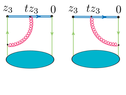
Figure 1: Coordinate representation for diagrams producing a large one-loop correction.

The term with $[\ln(1-w)]/(1-w)$ produces a large negative contribution. In Feynman gauge, according to Ref. Radyushkin:2017lvu , it comes from the evolution part of the vertex diagrams involving the gauge link (see Fig.1). The key point is that the gluon is attached there to a running $tz_{3}$ position on the link. After integration over $t$, etc., the net outcome is that the $z_{3}$-dependence of these diagrams is generated by an effective scale smaller than $z_{3}$. Indeed, let us combine the $[\ln(1-w)]/(1-w)$ term with the $\ln z_{3}^{2}$ logarithm by rewriting Eq. (17) as

$${\cal I}(\nu,\mu^{2})= {\mathfrak{M}}(\nu,z_{3}^{2})+\frac{\alpha_{s}}{\pi}\,C_{F}\,\int_{0}^{1}dw\,{\mathfrak{M}}(w\nu,z_{3}^{2})$$

$$\times\Biggl{\{}\frac{1+w^{2}}{1-w}\,\ln\left[(1-w)z_{3}\mu\frac{e^{\gamma_{E}+1/2}}{2}\right]$$

$$+\left[(w+1)\ln(1-w)-(1-w)\right]\Biggr{\}}_{+}\ .$$ (18)

We see that $z_{3}$ enters now through a running $(1-w)z_{3}$ location. The remaining $(w+1)\ln(1-w)$ term is much less singular than $B(w)$ for $w=1$, and does not produce large contributions.

Thus, the magnitude of the one-loop correction is governed by the combined evolution logarithm. It cannot be made zero by a particular choice of $\mu$ because it depends on the integration variable $w$. Still, the $w$-integrated contribution will vanish for some $\mu$ that we may write as

$$\mu=\frac{2e^{-1/2-\gamma_{E}}}{\langle 1-w\rangle}\,\frac{1}{z_{3}}\ ,$$ (19)

where $\langle 1-w\rangle$ is the “average” value of $1-w$. Since $B(w)$ is strongly enhanced for $w=1$, we should expect that $\langle 1-w\rangle$ is numerically small, leading to a $\mu\sim k/z_{3}$ rescaling with a rather large coefficient $k$. As we will see, $k\sim 4$ in this case.

Again, one may ask if the perturbative formula (17) involving the $\ln z_{3}^{2}$ logarithm may be applied to actual lattice data. In particular, our exercise with the mass-term IR regularization and the resulting Bessel function shows that the logarithmic behavior $\ln z_{3}^{2}$ of the hard term is valid only for $z_{3}$ values well below the IR cut-off $R$, which is given by the hadron size in our case. Hence, a practical question is whether the data really show a logarithmic evolution behavior in some region of small $z_{3}$.

IV Evolution in lattice data

IV.1 General features

An exploratory lattice study of the reduced pseudo-ITD ${\mathfrak{M}}(\nu,z_{3}^{2})$ for the valence $u_{v}-d_{v}$ parton distribution in the nucleon has been reported in Ref. Orginos:2017kos . An amazing observation made there was that, when plotted as functions of $\nu$, the data both for real and imaginary parts lie close to respective universal curves. The data show no polynomial $z_{3}$-dependence for large $z_{3}$. Given that $z_{3}^{2}/a^{2}$ changes in the explored range from 1 to about 200, we interpret this result as the total absence of higher-twist terms in the reduced pseudo-ITD.

As explained in Refs. Radyushkin:2017cyf ; Orginos:2017kos and in the Introduction, such an outcome corresponds to a factorization of the $\nu$- and $z_{3}^{2}$-dependences of the soft part of the Ioffe-time distribution ${\cal M}(\nu,z_{3}^{2})=M(\nu){\cal M}(0,z_{3}^{2})$. In terms of TMD ${\cal F}(x,k_{\perp}^{2})$, this corresponds to factorization of its $x$- and $k_{\perp}^{2}$-dependences in the region of soft $k_{\perp}$. However, as observed in Ref. Orginos:2017kos , there is quite visible $z_{3}$-dependence for small values of $z_{3}$, namely, $z_{3}\lesssim 6a$, that may be explained by perturbative evolution.

Let us consider first the real part. It corresponds to the cosine Fourier transform

$${\mathfrak{R}}(\nu)\equiv{\rm Re}\,{\mathfrak{M}}(\nu)= \int_{0}^{1}dx\,\cos(\nu x)\,q_{v}(x)$$ (20)

of the function $q_{v}(x)$ corresponding to the valence combination, i.e., the difference $q_{v}(x)=q(x)-\bar{q}(x)$ of quark and antiquark distributions. In our case, $q=u-d$.

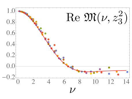
Figure 2: Real part of ${\mathfrak{M}}(\nu,z_{3}^{2})$ plotted as a function of $\nu=Pz_{3}$ and compared to the curve given by Eqs. (20), (21).

In Ref. Orginos:2017kos , it was found that the data for the real part are very close (see Fig. 2) to the curve ${\mathfrak{R}}_{f}(\nu)$ generated by the function

$$f(x)=\frac{315}{32}\sqrt{x}(1-x)^{3}\,.$$ (21)

This shape was obtained by forming cosine Fourier transforms of the normalized $x^{a}(1-x)^{b}$-type functions and fixing the parameters $a,b$ through fitting the data.

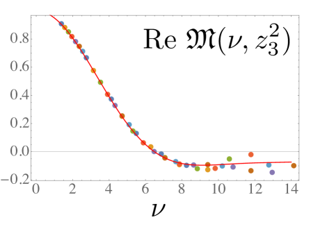
Figure 3: Real part of ${\mathfrak{M}}(\nu,z_{3}^{2})$ for $z_{3}$ ranging from $7a$ to $13a$.

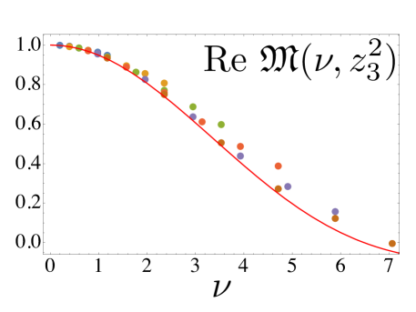
Figure 4: Real part of ${\mathfrak{M}}(\nu,z_{3}^{2})$ for $z_{3}$ ranging from $a$ to $6a$.

While all the data points have been used in the fit, the shape of the curve is obviously dominated by the points with smaller values of Re ${\mathfrak{M}}(\nu,z_{3}^{2})$. To give a more detailed illustration, we show in Fig. 3 the points corresponding to $z_{3}$ values in the range $7a\leq z_{3}\leq 13a$. As one can see, there is some scatter for the points with the largest values of $\nu$ in the region $\nu\gtrsim 10$, where the finite-volume effects become important. Otherwise, practically all the points lie on the universal curve based on $f(x)$. In this sense, there is no $z_{3}$-evolution visible in the large-$z_{3}$ data.

In Fig. 4, we show the points in the region $a\leq z_{3}\leq 6a$ (note that, on the lattice, $z_{3}=0$ means that also $\nu=0$, and ${\mathfrak{M}}(0,0)=1$ by definition). In this case, all the points lie higher than the universal curve. We recall that the perturbative evolution increases the real part of the pseudo-ITD when $z_{3}$ decreases. Thus, one may conjecture that the observed higher values of ${\mathfrak{R}}$ for smaller-$z_{3}$ points may be a consequence of the evolution.

A typical pattern of the $z_{3}$-dependence of the lattice points is shown in Fig. 5 for a “magic” Ioffe-time value $\nu=3\pi/4$ that may be obtained from five different combinations of $z_{3}$ and $P$ values used in Ref. Orginos:2017kos . The shape of the eye-ball fit line is given by the incomplete gamma-function $\Gamma(0,z_{3}^{2}/30a^{2})$. This function entirely conforms to the expectation that the $z_{3}$-dependence has a “perturbative” logarithmic $\ln(1/z_{3}^{2})$ behaviour for small $z_{3}$, and rapidly vanishes for $z_{3}$ larger than $6a$.

As expected, ${\mathfrak{R}}(\nu,z_{3}^{2})$ decreases when $z_{3}$ increases. We also see that the evolution “stops” for large $z_{3}$. In this context, the overall curve based on Eq. (21) corresponds to the “low normalization point”, i.e., to the region, where the perturbative evolution is absent.

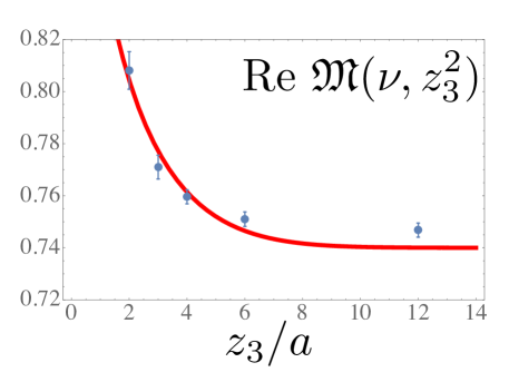
Figure 5: Dependence on $z_{3}$ for $\nu=3\pi/4\approx 2.3562$.

IV.2 Building $\overline{\rm MS}$ ITD

Thus, we see that the data of Fig. 5 show a logarithmic evolution behavior in the small $z_{3}$ region. Still, the $z_{3}$-behavior starts to visibly deviate from a pure logarithmic $\ln z_{3}^{2}$ pattern for $z_{3}\gtrsim 5a$. This sets the boundary $z_{3}\leq 4a$ on the “logarithmic region”. So, let us try to use Eq. (17) in that region to construct the $\overline{\rm MS}$ ITD.

It is instructive to split the contributions in Eq. (17), where we will denote ${\rm Re}\,{\cal I}(\nu,\mu^{2})\equiv{\cal I}_{R}(\nu,\mu^{2})$. The first, “evolution” part, given by

$${\cal I}^{\rm ev}_{R}(\nu,\mu^{2})= {\mathfrak{R}}(\nu,z_{3}^{2})+\frac{\alpha_{s}}{2\pi}\,C_{F}\,\int_{0}^{1}dw\,{\mathfrak{R}}(w\nu,z_{3}^{2})$$

$$\times B(w)\,\ln\left(z_{3}^{2}\mu^{2}\frac{e^{2\gamma_{E}}}{4}\right)\$$ (22)

(recall that ${\mathfrak{R}}(\nu,z_{3}^{2})\equiv{\rm Re}\,{\mathfrak{M}}(\nu,z_{3}^{2}$)) corresponds to the leading logarithm approximation used in Ref. Orginos:2017kos . For $z_{3}=2e^{-\gamma_{E}}/\mu$, the logarithm vanishes, and we have

$${\cal I}^{\rm ev}_{R}(\nu,\mu^{2})= {\mathfrak{R}}(\nu,(2e^{-\gamma_{E}}/\mu)^{2})={\mathfrak{R}}(\nu,(1.12/\mu)^{2})\ .$$ (23)

This happens, of course, only if, for an appropriately chosen $\alpha_{s}$, the $\ln z_{3}^{2}$-dependence of the one-loop correction cancels the actual $z_{3}^{2}$-dependence of the data, visible as scatter in the data points in Fig. 4. In Ref. Orginos:2017kos , it was found that this happens when $\alpha_{s}/\pi\approx 0.1$. Thus, Eq. (17) is accurate only in the region, where the data show a logarithmic dependence on $z_{3}$, i.e., $z_{3}\leq 4a$ in our case.

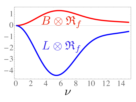
Figure 6: Functions $B\otimes{\mathfrak{R}}_{f}$ (upper line) and $L\otimes{\mathfrak{R}}_{f}$ (lower line) of Eq. (24).

Since the difference between ${\mathfrak{R}}(w\nu,z_{3}^{2})$ and ${\mathfrak{R}}_{f}(w\nu)$ is ${\cal O}(\alpha_{s})$, we may replace ${\mathfrak{R}}(w\nu,z_{3}^{2})$ by ${\mathfrak{R}}_{f}(w\nu)$ in Eq. (22) (recall that ${\mathfrak{R}}_{f}(\nu)$ corresponds to the PDF of Eq. (21)). The remaining part of ${\cal I}(\nu,\mu^{2})$ (where we have already substituted ${\mathfrak{R}}(w\nu,z_{3}^{2})$ by ${\mathfrak{R}}_{f}(w\nu)$)

$${\cal I}^{\rm NL}_{R}(\nu)= \frac{\alpha_{s}}{2\pi}\,C_{F}\,\int_{0}^{1}dw\,{\mathfrak{R}}_{f}(w\nu)$$

$$\times\left\{B(w)\,+\left[4\,\frac{\ln(1-w)}{1-w}-2(1-w)\right]_{+}\right\}$$

$$\equiv\frac{\alpha_{s}}{2\pi}\,C_{F}\,\left[B\otimes{\mathfrak{R}}_{f}+L\otimes{\mathfrak{R}}_{f}\right]\$$ (24)

is due to corrections beyond the leading logarithm approximation.

As we have discussed, the $L\otimes{\mathfrak{R}}_{f}$ term reflects the fact that the actual scale in the evolution part of the vertex diagrams is less than $z_{3}$. To illustrate its impact, we show, in Fig. 6, the functions $B\otimes{\mathfrak{R}}_{f}$ and $L\otimes{\mathfrak{R}}_{f}$. One can see that the last one is negative and rather large. Its $\nu$-dependence is similar to that of the $B\otimes{\mathfrak{R}}_{f}$ function. In fact, in the $\nu<5$ region, we have $L\otimes{\mathfrak{R}}_{f}\approx-3.5B\otimes{\mathfrak{R}}_{v}$. Thus, the combined effect of these two terms is close to that of $-2.5B\otimes{\mathfrak{R}}_{f}$. As a result, the inclusion of these terms may be approximately treated as a LLA evolution with a modified rescaling factor. Specifically, we may write

$${\cal I}_{R}(\nu,\mu^{2})\approx \,{\mathfrak{R}}(\nu,(2e^{1.25-\gamma_{E}}/\mu)^{2})\approx\,{\mathfrak{R}}(\nu,(4/\mu)^{2})\ .$$ (25)

Thus, the rescaling factor has changed by a factor of 4 compared to the original LLA value!

We may use $\mu\approx 4/z_{3}$ as a guide, but the actual numerical calculations should, of course, be done using the “exact” Eq. (17). To proceed, we choose the value $\mu=1/a$ which, at the lattice spacing of $0.093$ fm used in Ref. Orginos:2017kos is approximately 2.15 GeV. The estimate (25) tells us that the ITD ${\cal I}_{R}(\nu,\mu^{2})$ at this scale should be close to the pseudo-ITD ${\mathfrak{R}}(\nu,z_{3}^{2})$ for $z_{3}\approx 4a$, a distance that is on the border of the $z_{3}\leq 4a$ region. Taking the value $\alpha_{s}/\pi=0.1$ used in Ref. Orginos:2017kos and applying the full one-loop relation (17) to the data with $z_{3}\leq 4a$, we generate the points for ${\cal I}_{R}(\nu,(1/a)^{2})$.

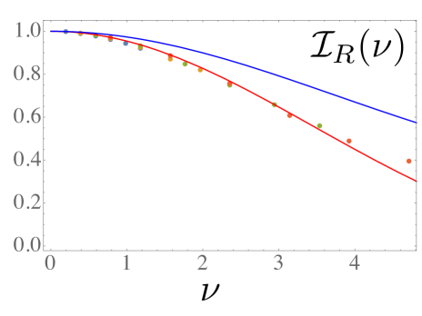
Figure 7: Function ${\cal I}_{R}(\nu,\mu^{2})$ for $\mu=1/a$ calculated using the data with $z_{3}$ from $a$ to $4a$. The upper curve corresponds to the ITD of the CJ15 global fit PDF.

As seen from Fig. 7, all the points are close to some universal curve with a rather small scatter. The curve itself was obtained by fitting the points by the cosine transform of a normalized $Nx^{a}(1-x)^{b}$ distribution, which gave $a=0.35$ and $b=3$. The magnitude of the scatter illustrates the error of the fit for the ITD in the $\nu\leq 4$ region. In Fig. 7, we compare our $\mu=1/a$ ITD with the ITD obtained from the global fit PDFs corresponding to the CJ15 Accardi:2016qay global fit. One can see that our ITD is systematically below the curve based on the global fit PDFs.

The reason for the discrepancy may be understood from Fig. 8, where we compare the normalized $Nx^{0.35}(1-x)^{3}\equiv q_{v}(x,\mu=2.15$ GeV) distribution to CJ15 Accardi:2016qay and MMHT 2014 Harland-Lang:2014zoa global fit PDFs, taken at the scale $\mu=2.15$ GeV. Unlike the $\sim x^{0.35}$ function, these PDFs are singular for small $x$, which leads to the enhancement of ITDs for large and moderate values of $\nu$.

To fit the points for ${\cal I}_{R}(\nu,\mu^{2})$, we have used the same simplest $Nx^{a}(1-x)^{b}$ Ansatz for the PDF as in Ref. Orginos:2017kos . In principle, one may use more complicated models for PDFs and get practically the same fitted curve for the ITD in the $\nu\leq 4$ region, while a somewhat different curve for PDF $q_{v}(x)$. The reason is simple: the inverse cosine Fourier transform is unique only when one exactly knows the ITD in the whole $0\leq\nu<\infty$ region. Performing such a transform from a limited $\nu\leq 4$ region, one needs to add some assumptions either about the behavior of the ITD outside this region or about a functional form of the PDF $q_{v}(x)$. We fixed our choice by taking $q_{v}(x)\sim x^{a}(1-x)^{b}$. The study of how the shape of $q_{v}(x)$ varies if one uses more complicated forms, in particular, those used in the global fits Accardi:2016qay ; Harland-Lang:2014zoa is an interesting problem that, however, goes beyond the scope of the present paper.

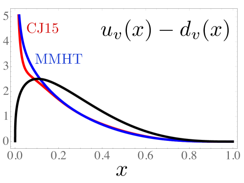
Figure 8: Curve for $u_{v}(x)-d_{v}(x)$ at $\mu=2.15$ GeV built from the data shown in Fig. 7 and compared to CJ15 and MMHT global fits.

Comparing to the LLA results of Ref. Orginos:2017kos , we observe that the large negative one-loop correction in Eq. (17) has visibly changed the extracted PDF, which is now further from the global fit PDFs. The main reason is that the $z_{0}=2a$ pseudo-ITD constructed in Ref. Orginos:2017kos was treated there as corresponding to the $\mu\approx 1$ GeV scale, while according to the modified rescaling relation (25), it should correspond to $\mu\approx 4$ GeV. Hence, to get the $\mu\approx 2$ GeV curve, one needs to evolve it down in $\mu$.

Still, the guiding idea of Ref. Orginos:2017kos , that the $\overline{\rm MS}$ ITDs ${\cal I}_{R}(\nu,\mu^{2})$ can be obtained from the reduced pseudo-ITDs ${\mathfrak{R}}(\nu,z_{3}^{2})$ by an appropriate rescaling $\mu=k/z_{3}$, works with a rather good accuracy for all $z_{3}\leq 6a$ if one takes $k\approx 4$. By this rescaling relation, the $\mu=1/2a\approx 1$ GeV ITD corresponds to the $z_{3}\approx 8a$ reduced pseudo-ITD. As we discussed, a boundary point beyond which the evolution stops, is $z_{3}\approx 6a$. Hence, the pseudo-ITD at this distance is given by the ITD ${\mathfrak{R}}_{f}(\nu)$ corresponding to the universal fit function $f(x)$ of Eq. (21). This result may be also obtained by a direct numerical calculation based on Eq. (17).

Using Eq. (17) one may also evolve the $\overline{\rm MS}$ ITD below $\mu=1/2a$, and the resulting functions will be changing with $\mu$. On the other hand, the pseudo-ITDs do not change with $z_{3}$ when $z_{3}\gtrsim 6a$. Hence, the rescaling connection ${\cal I}_{R}(\nu,\mu^{2})\approx{\mathfrak{R}}(\nu,(4/\mu)^{2})$ in this region becomes less and less accurate when $\mu$ decreases, and eventually makes no sense.

IV.3 Imaginary part

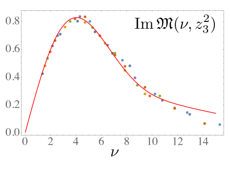
Figure 9: Imaginary part of ${\mathfrak{M}}(\nu,z_{3}^{2})$ for $z_{3}$ ranging from $7a$ to $13a$. The curve corresponds to $q(x)+\bar{q}(x)=f(x)+2\bar{q}(x)$, with $f(x)$ given by Eq. (21) and $\bar{q}(x)$ given by Eq. (27)

Imaginary part of the pseudo-ITD may be considered in a similar way. It corresponds to the sine Fourier transform

$${\rm Im}\,{\mathfrak{M}}(\nu)= \int_{0}^{1}dx\,\sin(\nu x)\,[q(x)+\bar{q}(x)]$$ (26)

of the function given by the sum $q(x)+\bar{q}(x)$ of quark and antiquark distributions. This function differs from the valence combination $q_{v}(x)=q(x)-\bar{q}(x)$ by $2\bar{q}(x)=2[\bar{u}(x)-\bar{d}(x)]$. In Fig. 9, we show the data for large $z_{3}$ values $z_{3}\geq 7a$. Just like in the case of the real part (see Fig. 3), the points with $\nu\lesssim 10$ are close to a universal curve. Representing $q(x)+\bar{q}(x)=q_{v}(x)+2\bar{q}(x)$ and taking $f(x)$ of Eq. (21) as $q_{v}(x)$, we find

$$\bar{q}(x)\approx 0.1\,[20x\,(1-x)^{3}]\,.$$ (27)

Note that in Ref. Orginos:2017kos , the fit was made for all the $z_{3}$ points (i.e. the points with $z_{3}\leq 6a$ have been also included), and the overall coefficient for $\bar{q}(x)$ was obtained to be 0.07 rather than 0.1.

In Fig. 10, we show data with $z_{3}\leq 4a$. As one can see, all these points are below the curve obtained by fitting the $z_{3}\geq 7a$ data. This is in agreement with the fact that, in the region $\nu\lesssim 6$, the perturbative evolution decreases the imaginary part of the pseudo-ITD when $z_{3}$ decreases. Note that the 1-loop relation holds for the whole function ${\mathfrak{M}}={\rm Re}\,{\mathfrak{M}}+i\,{\rm Im}\,{\mathfrak{M}}$. So, we should just separate there real and imaginary parts, and the construction of the $\overline{\rm MS}$ function ${\rm Im}\,{\cal I}(\nu,\mu^{2})\equiv{\cal I}_{I}(\nu,\mu^{2})$ proceeds in the same way as for the real part.

The results are shown in Fig. 11. Again, all the points are rather close to a universal curve with a rather small scatter. The curve shown corresponds to the sine Fourier transform of the sum of the valence distribution $q_{v}(x,\mu=1/a)=Nx^{0.35}(1-x)^{3}$ obtained from the study of the real part, and the antiquark contribution $2\bar{q}(x,\mu=1/a$). The latter was found from the fit to be given by $\bar{q}(x,\mu=1/a=2.15$ GeV) $=0.07[20x(1-x)^{3}]$.

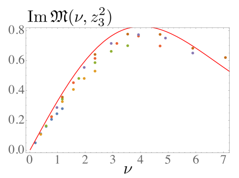
Figure 10: Imaginary part of ${\mathfrak{M}}(\nu,z_{3}^{2})$ for $z_{3}$ ranging from $a$ to $6a$. The curve is the same as in Fig. 9.

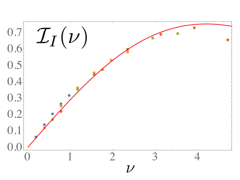
Figure 11: Function ${\cal I}_{I}(\nu,\mu^{2})$ for $\mu=1/a$ calculated using the data with $z_{3}$ from $a$ to $4a$. The curve is described in the text.

V Summary and conclusions

In this paper, we have extended the leading-logarithm analysis of lattice data for parton pseudo-distributions and reduced pseudo-ITDs performed in Ref. Orginos:2017kos . To this end, we incorporated recent results for the reduced pseudo-ITDs at the one-loop level Radyushkin:2017lvu (see also Ji:2017rah ; Izubuchi:2018srq ).

It was found that the correction contains a large term resulting in essential numerical changes compared to the LLA. The large correction appears since effective distances involved in the most important diagrams are much smaller than the nominal distance $z_{3}$. This leads to a change (from $k_{\rm LLA}\approx 1$ to $k\approx 4$ in the case of our particular ITDs) of the coefficient $k$ in the rescaling relation $\mu=k/z_{3}$ that allows to (approximately) convert the pseudo-PDFs ${\cal P}(x,z_{3}^{2})$ into the $\overline{\rm MS}$ PDFs $f(x,\mu^{2})$.

While the rescaling relation serves as an instructive guide for quick estimates and semi-quantitative analysis, the $\overline{\rm MS}$ ITDs may be directly constructed applying the exact one-loop formula. Using it, we have obtained the ITD ${\cal I}(\nu,\mu^{2})$ at the $\mu=1/a\approx 2.15$ GeV $\overline{\rm MS}$ scale using the data in the $0\leq z_{3}\leq 4a$ region.

We found that ${\cal I}(\nu,\mu^{2})$ at this scale is close to the reduced pseudo-ITD ${\mathfrak{M}}(\nu,z_{3}^{2})$ for $z_{3}\sim 4a$. Since all the data in the $a\leq z_{3}\leq 4a$ region do not differ much from the $z_{3}=4a$ ones (see Fig. 4), the conversion of the ${\mathfrak{M}}(\nu,z_{3}^{2})$ data into ${\cal I}(\nu,1/a^{2})$ does not involve large changes, i.e., the perturbative expansion for $\overline{\rm MS}$ ITD ${\cal I}(\nu,\mu^{2})$ in terms of the reduced pseudo-ITDs ${\mathfrak{M}}(\nu,z_{3}^{2})$ is under control. A formal reason is that the large correction in this case can be absorbed into the $z_{3}^{2}$-dependent evolution term, with remaining corrections being small.

Phenomenologically, the PDF extracted in this way follows the trend of those given by the global fits in the $x>0.1$ region, but does not reproduce their singular behavior in the $x<0.1$ region. The latter is usually related to the $x^{-0.5}$ pattern of the $\rho$-meson Regge trajectory. Since the $\rho$-meson is essentially a rather narrow resonance in the $\pi\pi$ system, one should not expect to accurately reproduce the $\rho$-meson properties in a lattice simulation in which the pions are as heavy as 600 MeV. Thus, one may hope that using simulations at physical pion mass would produce a better agreement with the global fits in the small-$x$ region. This hope is supported by recent extractions Alexandrou:2018pbm ; Chen:2018xof of $q_{v}(x)$ using the quasi-PDF lattice simulations at physical pion mass.