Galactic cold cores IX. Column density structures and radiative-transfer modelling

Abstract

Context. The $Galactic$ $Cold$ $Cores$ (GCC) project has made $Herschel$ photometric observations of interstellar clouds where $Planck$ detected compact sources of cold dust emission. The fields are in different environments and stages of star formation.

Aims. Our aim is to characterise the structure of the clumps and their parent clouds, and to study the connections between the environment and the formation of gravitationally bound objects. We also examine the accuracy to which the structure of dense clumps can be determined from sub-millimetre data.

Methods. We use standard statistical methods to characterise the GCC fields. Individual clumps are extracted using column density thresholding. Based on sub-millimetre measurements, we construct a three-dimensional radiative transfer (RT) model for each field. These are used to estimate the relative radiation field intensities, to probe the clump stability, and to examine the uncertainty of column density estimates. We examine the structural parameters of the clumps, including their radial column density profiles.

Results. In the GCC fields, the structure noise follows the relations previously established at larger scales and in lower-density clouds. The fractal dimension has no significant dependence on column density and the values $D_{\rm P}=1.25\pm 0.07$ are only slightly lower than in typical molecular clouds. The column density probability density functions (PDFs) exhibit large variations, for example, in the case of externally compressed clouds. At scales $r>0.1$ pc, the radial column density distributions of the clouds follow an average relation of $N\sim r^{-1}$. In spite of a great variety of clump morphologies (and a typical aspect ratio of 1.5), clumps tend to follow a similar $N\sim r^{-1}$ relation below $r\sim 0.1$ pc. RT calculations indicate only factor 2.5 variation in the local radiation field intensity. The fraction of gravitationally bound clumps increases significantly in regions with $A_{\rm V}>5$ mag but most bound objects appear to be pressure-confined.

Conclusions. The host clouds of the cold clumps in the GCC sample have statistical properties similar to general molecular clouds. The gravitational stability, peak column density, and clump orientation are connected to the cloud background while most other statistical clump properties (e.g. $D_{\rm P}$ and radial profiles) are insensitive to the environment. The study of clump morphology should be continued with a comparison with numerical simulations.

Table 1: List of Herschel fields. The columns are: (1) name of the field, (2)-(3) centre coordinates, (4) estimated distance, (5)-(6) size of the modelled region in arcmin and in 9$\arcsec$ pixels, (8)-(9) Plummer parameters of the default LOS density profile.

Field	RA	DEC	Distance	Model size		$A_{\rm V}^{\rm BG}$	$R$	$p$
	(J2000.0)	(J2000.0)	(pc)	(arcmin)	(pixels)	(mag)	(arcmin)
(1)	(2)	(3)	(4)	(5)	(6)	(7)	(8)	(9)
G0.02+18.02	16 40 56.7	-18 35 03.7	160	28.1	187$\times$187	0.5	2.9	2.4
G0.49+11.38	17 04 41.9	-22 13 52.3	160	35.1	234$\times$234	0.7	1.3	3.3
G1.94+6.07	17 27 50.7	-24 01 54.2	145	40.0	267$\times$267	1.6	11.5	8.1
G2.83+21.91	16 34 41.2	-14 09 27.4	300	38.1	254$\times$254	0.6	1.8	2.1
G3.08+9.38	17 17 29.6	-21 22 16.4	160	42.0	280$\times$280	0.7	1.1	1.8
G3.72+21.02	16 39 45.9	-14 02 09.3	160	40.0	267$\times$267	0.6	0.6	1.8
G4.18+35.79	15 53 43.4	-04 40 55.9	110	35.1	234$\times$234	0.5	2.7	3.6
G6.03+36.73	15 54 05.9	-02 54 39.7	110	35.1	234$\times$234	0.4	0.7	2.2
G9.45+18.85	17 00 22.2	-10 53 06.1	280	40.0	267$\times$267	0.6	4.7	2.9
G20.72+7.07	18 03 38.9	-07 30 25.0	260	30.0	200$\times$200	1.3	0.8	1.8
G21.26+12.11	17 46 47.7	-04 38 48.1	120	35.1	234$\times$234	0.9	-0.5	2.3
G24.40+4.68	18 19 21.5	-05 29 45.1	260	36.0	240$\times$240	1.7	0.8	2.1
G25.86+6.22	18 16 32.7	-03 23 49.4	260	36.0	240$\times$240	3.1	0.6	1.9
G26.34+8.65	18 08 37.9	-01 51 26.6	400	30.0	200$\times$200	1.3	1.0	3.6
G93.21+9.55	20 37 00.2	+56 58 46.8	440	30.0	200$\times$200	0.9	-0.4	2.5
G108.28+16.68	21 10 13.4	+72 52 58.5	300	35.1	234$\times$234	0.6	0.9	2.1
G110.62-12.49	23 37 39.8	+48 31 40.4	440	40.0	267$\times$267	0.2	0.6	2.6
G110.80+14.16	21 59 02.5	+72 52 56.0	400	40.0	267$\times$267	0.7	0.5	1.9
G116.08-2.40	23 57 06.7	+59 43 26.9	500	30.0	200$\times$200	1.3	0.8	2.3
G126.63+24.55	04 19 14.0	+85 52 06.5	125	30.0	200$\times$200	0.2	2.3	4.6
G141.25+34.37	08 48 58.2	+72 41 16.1	110	40.0	267$\times$267	0.1	1.2	1.8
G149.67+3.56	04 17 53.6	+55 15 05.2	170	40.0	267$\times$267	1.6	1.5	2.2
G150.47+3.93	04 24 37.8	+54 58 21.4	170	40.0	267$\times$267	1.7	-0.3	1.9
G151.45+3.95	04 29 53.9	+54 16 52.5	170	36.0	240$\times$240	1.2	3.5	2.6
G154.08+5.23	04 47 34.4	+53 05 02.4	170	34.0	227$\times$227	1.2	-0.5	2.4
G155.80-14.24	03 36 49.2	+37 42 31.1	350	40.0	267$\times$267	0.5	0.6	2.1
G157.08-8.68	04 01 55.7	+41 15 20.4	150	40.0	267$\times$267	1.1	0.5	2.1
G159.23-34.51	02 55 54.0	+19 37 10.2	325	40.0	267$\times$267	0.6	0.8	2.0
G161.55-9.30	04 16 06.1	+37 49 20.2	250	36.0	240$\times$240	0.8	0.8	2.0
G163.82-8.44	04 29 00.9	+36 43 21.1	420	50.1	334$\times$334	1.4	-0.4	2.1
G164.71-5.64	04 40 58.0	+37 59 06.6	330	42.0	280$\times$280	1.3	1.2	1.9
G167.20-8.69	04 36 34.8	+34 16 53.3	160	40.0	267$\times$267	0.9	0.5	1.8
G173.43-5.44	05 08 32.7	+31 26 38.8	150	45.0	300$\times$300	0.9	1.5	2.5
G181.84-18.46	04 44 00.3	+16 57 22.7	500	36.0	240$\times$240	0.7	1.4	2.8
G188.24-12.97	05 17 05.1	+14 59 33.2	445	40.0	267$\times$267	0.6	0.8	1.6
G189.51-10.41	05 29 55.2	+15 25 03.2	445	42.0	280$\times$280	0.6	0.5	2.1
G198.58-9.10	05 52 53.1	+08 22 34.1	450	35.1	234$\times$234	0.7	1.1	4.0
G203.42-8.29	06 04 47.6	+04 20 31.3	390	44.1	294$\times$294	0.7	1.6	3.6
G205.06-6.04	06 16 27.5	+04 07 44.0	400	44.1	294$\times$294	0.8	1.3	2.1
G206.33-25.94	05 07 01.2	-06 17 56.6	210	35.1	234$\times$234	0.1	0.8	2.6
G210.90-36.55	04 34 54.6	-14 23 35.1	140	50.1	334$\times$334	0.5	4.0	5.3
G212.07-15.21	05 55 49.7	-06 11 25.9	230	36.0	240$\times$240	0.6	1.3	2.0
G247.55-12.27	07 09 26.3	-36 16 39.6	170	44.1	294$\times$294	0.5	1.9	2.0
G298.31-13.05	11 39 22.1	-75 14 27.0	150	25.1	167$\times$167	0.5	1.1	2.6
G300.61-3.13	12 28 54.8	-65 47 40.5	200	36.0	240$\times$240	1.2	1.9	3.0
G300.86-9.00	12 25 17.0	-71 43 05.5	150	36.0	240$\times$240	0.7	1.3	3.1
G315.88-21.44	17 19 39.9	-76 55 17.2	250	35.1	234$\times$234	0.2	0.7	2.2
G341.18+6.51	16 25 05.1	-39 59 10.4	140	25.1	167$\times$167	1.4	3.2	6.2
G344.77+7.58	16 33 30.3	-36 39 02.1	240	40.0	267$\times$267	0.9	-0.5	2.4
G345.39-3.97	17 23 01.0	-43 26 24.7	225	33.0	220$\times$220	0.9	-0.5	3.0
G358.96+36.75	15 39 50.0	-07 12 09.0	110	35.1	234$\times$234	0.2	1.8	2.2

1 Introduction

The all-sky survey of the Planck satellite (Tauber et al. 2010) made it possible to catalogue cold interstellar clouds at a Galactic scale. The angular resolution of $\sim 5\arcmin$ in the Planck sub-millimetre bands allowed the identification of compact sources that are associated with the early phases of star formation. Analysis of Planck data led to the creation of the Cold Clump Catalogue of Planck Objects (PGCC, see Planck Collaboration et al. 2016b), which lists basic properties of over 13000 sources. The low colour temperatures (mostly $T\la 14$ K) are a direct indicator of the presence of high-column density structures. The objects are only partially resolved by the Planck beam. Therefore, the catalogued objects, generally referred to as clumps, are likely to contain substructure, including gravitationally bound prestellar and protostellar cores.

The Herschel Open Time Key Programme Galactic Cold Cores (GCC) carried out continuum observations of 116 fields selected from an early version of the Planck C3PO catalogue (Planck Collaboration XXIII 2011). The fields were mapped with Herschel PACS and SPIRE instruments (Pilbratt et al. 2010; Poglitsch et al. 2010; Griffin et al. 2010) between 100 and 500 $\mu$m, the data enabling the study of the Planck clumps at up to $\sim$20 times higher spatial resolution (Juvela et al. 2010; Planck Collaboration et al. 2011b; Juvela et al. 2012; Montillaud et al. 2015; Juvela et al. 2015a). Typically the Herschel maps are some $40\arcmin$ in size and contain a few $Planck$ clumps and also observations of their environment. This is useful for studies of dust property variations (Juvela et al. 2011, 2012, 2015b, 2015a) but also makes it possible to trace density structures from gravitationally bound cores to clumps and filaments, the parental molecular cloud, and sometimes even all the way to the surrounding diffuse medium (Juvela et al. 2012; Montillaud et al. 2015). Studies have already been carried out on the structure of filaments (Rivera-Ingraham et al. 2016, 2017) and high-latitude clouds, especially the cloud LDN 1642 (Malinen et al. 2014, 2016), and the kinematics (e.g. the internal turbulence of the clumps) through molecular line observations (Parikka et al. 2015; Fehér et al. 2017; Saajasto et al. 2017).

Column densities can be estimated from dust emission but only assuming that the properties of the emitting dust grains are known. The accuracy of the estimates is limited by the uncertainty and the spatial variations of dust opacity, $\kappa$, and to a lesser extent by the dust opacity spectral index, $\beta$. The sub-millimetre dust opacity $\kappa$ is likely to vary between low- and high-density regions (e.g. Stepnik et al. 2003; Lehtinen et al. 2007; Paradis et al. 2009; Martin et al. 2012; Ysard et al. 2013; Roy et al. 2013; Juvela et al. 2015b), which increases the uncertainty of mass estimates and could cause systematic errors in the estimated filament, clump, and core profiles. The dust opacity spectral index $\beta$ is also believed to increase towards the coldest regions (Désert et al. 2008; Dupac et al. 2003; Paradis et al. 2010; Planck Collaboration et al. 2011a; Planck Collaboration XI 2014; Schnee et al. 2014; Juvela et al. 2015a), possibly partially cancelling out the bias caused by $\kappa$ variations. The true variations of $\kappa$ and $\beta$ are close to the sensitivity limit of current sub-millimetre observations. Therefore, also in this paper, the potential effects of $\beta$ and $\kappa$ changes are examined through a comparison of a couple of alternative scenarios.

Temperature variations along the line-of-sight (LOS) are another notable source of error that cause the column densities to be underestimated towards cold clumps (Shetty et al. 2009; Malinen et al. 2011; Juvela & Ysard 2012). The effect would thus be opposite to that of $\kappa$ variations, if $\kappa$ increases in the clumps above the value assumed in the analysis. For externally heated clouds with tens of magnitudes of visual extinction, this error can also even be a factor of several (Juvela et al. 2013; Pagani et al. 2015). The effect can be significantly reduced by internal heating sources (Malinen et al. 2011), which makes it even more unpredictable. For starless objects, it is possible to use radiative-transfer (RT) models to derive an approximate correction (Juvela et al. 2013, 2015b). It is clear that an accurate determination of real column densities and of real density profiles is essential when observations are compared to models of interstellar filaments or prestellar and protostellar cores.

In this paper, the emphasis is on density structures of clumps that are larger than the protostellar cores. If the clumps are prestellar, they are particularly interesting as an intermediate phase between the general turbulent density field and the later gravity-dominated development. The shapes and density profiles of the clumps should reflect the processes that lead to the creation of gravitationally bound objects. Depending on the region, the processes can include the random turbulent motions, larger-scale converging flows and cloud collisions, or more direct dynamic influences of stellar populations in the form of radiation pressure, ionisation shocks, and supernova remnants. Therefore, one can expect correlations between the properties of the clumps and their environment. The GCC sample is well suited for such studies because it contains a heterogeneous sample of objects from different Galactic environments.

In this paper, we examine the density structures of the GCC fields from individual clumps to the extent of entire $Herschel$ maps. We characterise the basic statistical properties of the identified clumps (e.g. aspect ratios and skewness) and extract their radial column density profiles. We use RT modelling to quantify the uncertainties caused by the cloud temperature structure and by the potential changes of dust-emission properties. Models also provide information on the differences in the local radiation field intensity. On the other hand, we characterise the general properties of the Herschel fields with standard statistical tools (e.g. structure noise, fractal dimensions, and column density probability density functions). We also look for correlations between the properties of the clumps and the large-scale cloud structure, for example, regarding the clump orientations and the general anisotropy of the column density field.

The structure of the paper is as follows. The observations are described in Sect. 2 and the main methods are listed in Sect. 3. The main results are presented in Sect. 4, including the basic statistical parameters of the extracted structures, the clump radial profiles, and gravitational stability of the clumps. We discuss the results in Sect. 5 before listing our main conclusions in Sect. 6.

2 Observations

In the GCC project, the fields for Herschel observations were selected based on Planck all-sky observations and ancillary data, with the intention of covering a representative set of objects in different Galactic environments. The target selection is described in Juvela et al. (2012) and an overview of the observations is given in Montillaud et al. (2015) and Juvela et al. (2015b). The sample does not include regions that were included in other Herschel key programmes (e.g. the Galactic plane $|b|<1^{\degr}$ covered by the Hi-GAL programme (Molinari et al. 2010) and the individual clouds covered by the Gould Belt survey (André et al. 2010) and HOBYS (Motte et al. 2010) programmes).

The GCC observations cover 116 fields. The maps observed with the SPIRE instrument correspond to wavelengths 250 $\mu$m, 350 $\mu$m and 500 $\mu$m. The maps have an average size of $\sim 1800$ arcmin². The fields are listed in Juvela et al. (2015a) Table 3 and the Herschel observation identification numbers can be found in Montillaud et al. (2015). We use data identical to those in Juvela et al. (2015a). The SPIRE observations were reduced with the Herschel Interactive Processing Environment HIPE v.12.0, using the official pipeline with iterative destriper, extended emission calibration options, and naive map-making. The raw and pipeline-reduced data are available via the Herschel Science Archive. The resolution of the maps is approximately 18$\arcsec$, 25$\arcsec$, and 37$\arcsec$ for 250, 350, and 500 $\mu$m, respectively. The data were colour corrected and zero-point corrected as explained in Juvela et al. (2015a). For SPIRE observations we adopt a 7% uncertainty of absolute calibration and a 2% uncertainty of relative calibration. In this paper, we analyse 51 fields that have estimated distances below or equal to 500 pc (see Table 1). The distance estimates are discussed in detail in Montillaud et al. (2015).

For the RT models, we extracted from each SPIRE map a rectangular area that was between $25\arcmin\times 25\arcmin$ and $50\arcmin\times 50\arcmin$ in size and covered the most interesting high-density regions. To match the cell size of the RT models (see below), the data were resampled onto 9.0$\arcsec$ pixels with the Montage package. The 250 $\mu$m data remain at their original resolution. The 350 $\mu$m and 500 $\mu$m data also were convolved with a 10.0$\arcsec$ Gaussian as they were resampled onto the pixels of the 250 $\mu$m maps. Convolution was used to mitigate aliasing effects caused by the different pixel locations of the different maps. We calculated dust optical depth maps directly via colour temperature, assuming a fixed value of $\beta$=1.8, applicable as an approximate average value over the fields (Juvela et al. 2015a). The colour temperatures (at a resolution of 40$\arcsec$) were used to colour correct the surface-brightness data. Optical-depth data in the percentile range 0.5-6.0% were used to select pixels that define the local background. The average values of these pixels were then used to carry out background subtraction for each surface-brightness map. The RT models describe this emission and, thanks to background subtraction, can be assumed to represent a finite volume in the LOS direction. The background-subtracted maps were used to derive new optical-depth maps via spectral energy distribution (SED) fitting and they also serve as the basis of modelling, describing monochromatic emission at the reference wavelengths and above diffuse emission. These maps are also independent of the zero point corrections that in the previous papers were calculated with the help of Planck data (Juvela et al. 2015b, a). Only the intermediate calculation of dust-temperature maps (before colour corrections) relies on absolute surface-brightness zero points that are the same as in Juvela et al. (2015a).

The effective point spread function (PSF) of SPIRE depends on the source spectrum. The RT models are intended to describe cloud structure at the resolution of SPIRE 250 $\mu$m data. Therefore, when models are compared with observations, the model predictions are convolved from the resolution of 250 $\mu$m map down to the resolution of 350 $\mu$m and 500 $\mu$m maps. The kernels for these convolutions were created adopting a temperature of 15.0 K and a spectral index of 1.8. As noted in Juvela et al. (2015a), for parameter ranges of $T\sim$10–20 K and $\beta\sim$1.5-2.5, the variation of the PSF shape is negligible.

3 Methods

In this Section we describe the extraction of structures from column density maps. We also describe the selection of clumps, their basic statistical analysis, and the derivation of the clump radial column density profiles. We start with the general properties of the fields before discussing the characterisation of individual clumps. Finally, the RT models are discussed in Sect. 3.2.

3.1 Characterisation of the fields

To study the large-scale ($>0.1$ pc) column density structures, we use a set of common statistics that are used to analyse cloud observations and especially far-infrared and sub-millimetre data. These include fractal dimensions, structure noise, and probability density functions (PDFs). Furthermore, we use template matching to quantify the angular distribution of elongated structures.

The fractal dimension of interstellar clouds has been studied across a wide range of size scales, down to the linear scales probed by our $Herschel$ observations. The presence of a single fractal dimension may be related to the scale-free nature of interstellar turbulence. However, with the increasing role of self-gravity, the behaviour might change at clump scales. We estimate the fractal dimension $D_{\rm P}$ from the relation between the perimeter $P$ and the surface area $A$, $P\propto A^{D_{\rm p}/2}$ (Mandelbrot 1983; Falgarone et al. 1991; Stutzki et al. 1998). Because $D_{\rm P}$ characterises the general cloud structure, it is not sensitive to the spatial data resolution. We use mainly the optical depth maps $\tau(250\mu{\rm})$ at 40$\arcsec$ resolution. The values of $D_{\rm P}$ are derived from 100 contours between the peak value and the 10% percentile of the pixel values. All contours that touch the map boundaries or enclose an area of less than 1.1 arcmin² are ignored.

The structure function describes signal fluctuations as a function of the spatial scale, in a way similar to the power spectrum analysis. Thus, it is also related to the forces forming the cloud structure (e.g. turbulence). The second-order structure function $S(\theta)$ is

$$S(\theta)=\langle|Y(x)-Y(x+\theta)|^{2}\rangle,$$ (1)

where $\theta$ is the spatial (angular) separation and $Y$ are the data values (in our case intensity or column density) and the averaging extends over all map pixels (Gautier et al. 1992). Each value $Y(x)$ is an average over a measurement aperture with a diameter $D$ or, in our case, over the beam ($D\sim$FWHM). The reference $|Y(x+\theta)|$ could be an average of values read from either side of the aperture, $(|Y(x+\theta)|+|Y(x-\theta)|)/2$, or from a reference annulus (Gautier et al. 1992; Kiss et al. 2001; Martin et al. 2010). We follow the first approach, using two reference positions.

The PDF analysis examines the probability distribution of surface brightness or column density values (e.g. Kainulainen et al. 2009; Schneider et al. 2015a). Observations and simulations of the density and column density of interstellar clouds have shown that the distribution often resembles a log-normal function (Vazquez-Semadeni 1994; Padoan et al. 1997). A power-law tail, sometimes observed at high column densities, has been attributed to the presence of gravitationally bound objects, although there may be other contributing factors (Klessen 2000; Kritsuk et al. 2011; Brunt 2015). We estimate the PDF functions of the column density maps, within the limitations set by the finite map sizes. For comparison, PDFs are also calculated for the 250 $\mu$m surface brightness data, which is more weighted towards the distribution of warm dust.

We use a template-matching method (TM) to measure the anisotropy of column density structures at a given size scale $F$. Template matching can be seen as a subset of pattern recognition methods. Instead of a single specific algorithm, one uses an image of the search pattern that is compared to the data (Brunelli 2009). Our procedure is described in detail in Juvela (2016). The analysis uses the difference between maps convolved with Gaussian beams with FWHM values of (for example) $F$ and $2\times F$, which separates structures within a limited range of spatial frequencies. In the second stage, data at each map position are compared to a pre-defined template, which is rotated to find the best match to the data. To match elongated structures, we use the same $3\times 3$ element template as in Juvela (2016), which can be represented with a matrix

$$\pmatrix{-}1/3&2/3-1/3\\ -1/32/3-1/3\\ -1/32/3-1/3\\ .$$ (2)

The significance of the match is calculated by multiplying the template values with the corresponding data values (for the current position and orientation of the template) and by summing the resulting values. The significance (goodness-of-fit) and the position angle giving the highest significance are registered as maps with dimensions identical to the input map. We count position angles counter-clockwise from the Equatorial north. The final result consists of position angle histograms. We first reject a certain percentage of pixels with the lowest significance values. This is sufficient for our purposes (for a qualitative description of the anisotropies) because the random position angles of low-significance pixels simply add a flat pedestal to the histograms.

In the basic TM method, the computed significance depends on the absolute pixel values and the result is weighted towards high-column density regions. We also use a variation where the data values under the current template are normalised by their standard deviation. This removes the dependence on absolute data values and enables the characterisation of structures even in the most diffuse parts of the fields (see Juvela 2016).

The TM method is not very sensitive to clumps although the pattern of Eq. (2) will give a positive output at the location of a spherically symmetric object. The signal could be strong for very bright objects. However, with the above-mentioned normalisation, even slightly elongated cores and clumps lead to a smaller significance than faint but more elongated filaments.

The fields (and clumps) will also be characterised by the presence of young stellar objects (YSOs). We use the compilation of YSO candidates presented in Montillaud et al. (2015).

3.2 Radiative-transfer models

We construct for each field a three-dimensional (3D) radiative-transfer model whose sub-millimetre emission matches the SPIRE observations. The main assumptions regarding the dust model, the radiation field, and the density field are listed below. The variations of the default models are summarised in Table 2

Table 2: Parameters of the default radiative-transfer models and the assumption differences in the alternative fits.

Model	Assumptions
$D$	default case, $\tau(250\mu{\rm m})/\tau(J)=1.0\times 10^{-3}$, $\beta=1.8$
$P$	$k_{\rm ISRF}$ fitted using pixels with highest 3% of $N({\rm H}_{2})$ only
$W$	LOS cloud extent adjusted pixel by pixel
$\Delta A_{\rm V}$	external field changed by $A_{\rm V}$=$\pm 1$ mag
$K$	$\tau(250\mu{\rm m})/\tau(J)=2.0\times 10^{-3}$, $\beta=2.1$
$TD$	dust changes with density from $D$ to $K$ assumptions

3.2.1 Dust models

The essential dust parameters are the sub-millimetre dust opacity $\kappa$, the dust opacity spectral index $\beta$, and the ratio of opacities at the wavelengths where dust absorbs (ultraviolet, optical, and near-infrared) and emits (far-infrared, sub-millimetre) most of energy. The dust opacity affects the dust temperature and, for a given temperature, the scaling between the column density and the surface brightness. In observations, $\beta$ is largely degenerate with dust colour temperature. However, in RT models the temperatures are solved self-consistently and the assumed value of $\beta$ has a more direct effect on the intensity ratios between bands.

We use dust models loosely based on the Draine (2003) dust model of Milky Way dust, with a value of the total-to-selective extinction ratio $R_{\rm V}=A_{\rm V}/E({\rm B}-{\rm V})=3.1$ and a gas-to-dust ratio of 124. However, we modify this assuming a constant value of $\beta$ at all wavelengths $\lambda\geq 30$ $\mu$m and explicitly specifying the optical depth ratio between 250 $\mu$m and the $J$ band. Juvela et al. (2015b) estimated that in the GCC fields the optical depth ratio $\tau(250\mu{\rm m})/\tau(J)$ is higher than in diffuse clouds, with a median value of $\sim 1.6\times 10^{-3}$. Juvela et al. (2015a) concluded that the average spectral index increases towards the coldest clumps of the GCC fields. The median far-infrared spectral index was found to be $\sim 1.9$, the values sometimes exceeding 2.0. Based on these findings, we use two alternative dust models. The first one has $\tau(250\mu{\rm m})/\tau(J)=1.0\times 10^{-3}$ and $\beta=1.8$ and the second one has $\tau(250\mu{\rm m})/\tau(J)=2.0\times 10^{-3}$ and $\beta=2.1$. These bracket most of the observed parameter range and should show the quantitative effects of dust property uncertainties. Conversely, this will give an idea of the accuracy to which these parameters can be constrained by observations. We will also briefly experiment with spatial variations of dust properties, which is implemented by varying, cell-by-cell, the relative abundance of the two dust species described above.

3.2.2 Radiation field

We start with the assumption that the model clouds are illuminated by an isotropic external field with intensities given in Mathis et al. (1983). This is rarely sufficient to match the observed dust colour temperatures. Therefore, the intensity of the radiation field is scaled with a factor $k_{\rm ISRF}$, which varies from field to field. In the first approximation, this is sufficient to match observations in regions with different levels of heating. However, also the spectral shape of the illuminating radiation is important. For example, if the radiation field contains less short-wavelength radiation, the temperature contrasts between low- and high-column density regions becomes smaller. The question is particularly relevant because we are modelling background-subtracted surface brightness values, that is, an inner region of a cloud that may be surrounded by an envelope with a non-negligible extinction. Because the modelled surface brightness data are also background-subtracted, the external radiation field should be attenuated by a dust layer that roughly corresponds to half of the full LOS column density of the reference areas. This is only a crude approximation and assumes that most of the material along LOS is actually around the dense cloud. To examine the effects of the attenuation of the external field, we test cases where the Mathis et al. (1983) field is modified by a term $exp(-\tau_{\nu})$, where the optical depth $\tau$ at the frequency $\nu$ corresponds to a visual extinction of $A_{\rm V}=\pm 1$ mag. Here the negative extinction simply means a radiation field with a stronger short wavelength part.

3.2.3 Model clouds

Each cloud is modelled using a 3D density grid. The grid is uniform in the plane of the sky (POS) with the cell size corresponding to the pixel size of the resampled observations, $\Delta=$9.0$\arcsec$. In equatorial coordinates the projected width and height of the maps, $N\times\Delta$, ranges from 20$\arcmin$ to 50$\arcmin$, depending on the SPIRE maps. The cell size was selected as a compromise between the run times (increasing as $N^{3}$) and the resolution required for comparison with observations. With $\Delta$=9.0$\arcsec$, the 250 $\mu$m observations with FWHM$\sim 18\arcsec$ (the highest-resolution data used in the model fitting) are still Nyquist sampled.

In the LOS direction the density distribution is unknown but we assume that it has a Plummer-like profile,

$$\rho=\frac{\rho_{\rm c}}{(1+(z/R)^{2})^{p/2}},$$ (3)

where $\rho_{\rm c}$ is the maximum density and $z$ is the distance from the symmetry plane that, in the LOS direction, is located half way through the cloud. The density profile has two parameters, $R$ describing the extent of a central flattened part and $p$ describing the steepness of the density drop at larger distances. These parameters were defined for each field separately by fitting a column density cross-section of the main clump (or a typical clump) along its minor axis with a corresponding Plummer column density profile and converting this into a function of density (see Arzoumanian et al. 2011, Eq. 1). Thus, the adopted LOS profile is most appropriate for the densest regions, where the cloud shape has the largest effect on dust temperatures. The procedure assumes that the LOS extent is similar to the smaller of the clump dimensions seen in the POS. This is appropriate for spherical clumps and cylindrical filaments. However, it will underestimate the LOS extent, for example, when a filament or an elongated clump is observed along its major axis. In the LOS direction, the RT calculations employ a non-uniform discretisation where the number of cells is 30% lower than in the other two dimensions. The cell size decreases towards the density peak ($z=0$) where it is equal to the resolution in the POS. This reduces the time and memory used for calculations, at the same time retaining sufficient resolution near the density peak.

Because the LOS extent of the cloud is poorly constrained, below we also examine models where the LOS scale is a free parameter. This is implemented using a parameter map $k_{\rm W}$ that, at the position of each map pixel, gives a linear scaling for the LOS width of the density profile. Thus, in Eq. (3), $R$ will be replaced with $R\times k_{\rm W}$.

3.2.4 Optimisation of the cloud models

The RT calculations were performed with SOC, a new Monte Carlo program (Juvela 2018) that has been compared with other RT codes (Gordon et al. 2017). Given a density distribution, a dust model, and an external radiation field, SOC solves the dust temperature in each cell and computes surface-brightness maps at the requested wavelengths. Because we analyse observations at wavelengths $\lambda>100\mu$m, stochastically heated grains have only a minor effect and our calculations assume that all grains remain in thermal equilibrium with the radiation field. The radiation field is estimated on a grid of 50 frequencies that extend logarithmically from 10¹¹ Hz to $3\times 10^{15}$ Hz. Each frequency is simulated with about 10⁶ photon packages. This results in information about the absorbed energy within each model cell and the integration over frequency provides the absorbed energy that is then used to calculate dust temperatures. With the employed number of photon packages, the Monte Carlo noise is below 0.1 K in terms of the dust temperature of individual cells. After the integration along the LOS and the convolution with the beam, the noise of the synthetic surface-brightness maps is several times below the uncertainty of the observed maps. Models give predictions of the monochromatic surface brightness at 250 $\mu$m, 350 $\mu$m, and 500 $\mu$m at the resolution of the 250 $\mu$m observations. These data are convolved to the resolution of the corresponding observed maps for the comparison with the measurements (see Sect. 2).

We optimise the models by scaling the model column densities, the intensity of the external radiation field, and optionally some additional parameters.

The intensity of the external radiation field is scaled by a single factor $k_{I}$. We do not consider changes in either the spectrum or the angular dependence of the incoming radiation. The parameter $k_{I}$ is updated based on the ratio between the 250 $\mu$m and 500 $\mu$m surface brightness,

$$k_{I}=\frac{I_{\rm Obs}(250\mu{\rm m})I_{\rm Mod}(500\mu{\rm m})}{I_{\rm Obs}(500\mu{\rm m})I_{\rm Mod}(250\mu{\rm m})}.$$ (4)

Because $k_{I}$ affects the whole model, we update it using average surface-brightness values over a large area. The averaged pixels are selected based on the optical depth $\tau_{\rm MBB}$ derived from the modified blackbody (MBB) fits of the observations. By default, we use pixels with $\tau_{\rm MBB}(250)$ between the 70% and 98% percentiles, thus concentrating more on the high-column density regions. The upper limit of 98% is used to reduce the effect of point sources. We also carry out complementary calculations where $k_{I}$ is determined by pixels in the 97.0-99.7% range of $\tau_{\rm MBB}(250)$. In this case, the radiation field is tuned to give a good fit exclusively to the densest clumps.

Apart from the radiation field, the observed surface brightness depends mainly on the line-of-sight column density. To match the surface-brightness variations on the plane of the sky, the column density is scaled pixel-by-pixel. The updates are done according to the ratio of the observed and modelled 350 $\mu$m surface brightness,

$$k_{N}^{i}=I_{\rm Obs}^{i}(350\mu{\rm m})/I_{\rm Mod}^{i}(350\mu{\rm m}).$$ (5)

The scaling applies equally to all cells along a LOS that correspond to the same map pixel. The procedure is not optimal, because the model column densities will mainly depend on a single frequency band. On the other hand, this enables a cleaner separation between column density and radiation field updates, which speeds up the optimisation.

Optionally, the LOS cloud profile can also be modified. One could use a single parameter to scale the cloud shape between oblate and prolate geometries. However, our fields typically consist of a number of separate clumps and the same scaling is not likely to work for all substructures. Therefore we adjust the LOS cloud extent with the parameter $k_{I}^{i}$ that is set for each map pixel $i$ separately. The updates are based on the ratios

$$k_{W}^{i}=\frac{I_{\rm Obs}^{i}(250\mu{\rm m})I_{\rm Mod}^{i}(500\mu{\rm m})}{I_{\rm Obs}^{i}(500\mu{\rm m})I_{\rm Mod}^{i}(250\mu{\rm m})}.$$ (6)

If the LOS extent is increased ($k_{W}>1.0$), the medium receives more radiation and the dust temperature increases. Thus the ratio in Eq. (6) again traces temperature changes, however, unlike in Eq. (4), the updates are not global but affect each LOS separately. There is some coupling between different LOS because of the mutual shadowing of the volume elements. In our models, the density always reaches its maximum in the central plane ($z$=0) of the model volume. If the cloud consisted of separate clumps at different $z$ locations, this would reduce the mutual shadowing of the clumps. In the models, this can be compensated by having a larger $k_{W}$ value.

The models do not include details such as radiation field anisotropy or internal sources. Even when these exist in the real data, the model results are valuable by explicitly showing these effects in their residuals. For partly the same reason, we do not directly use the column density maps from the models to correct the MBB values. We use the ratio $\xi_{N}$ between the actual column density of the model cloud and the column density that is estimated from the surface brightness produced by the model. This gives a more robust estimate of the relative bias in MBB analysis that is caused by LOS temperature variations. Thus, in addition to the original column density $N_{\rm obs}$ derived from observations via MBB fits, we will use bias-corrected column density maps $N_{\rm cor}=\xi_{N}\,N_{\rm obs}$. Figure 1 shows the field G150.47+3.93 as an example.

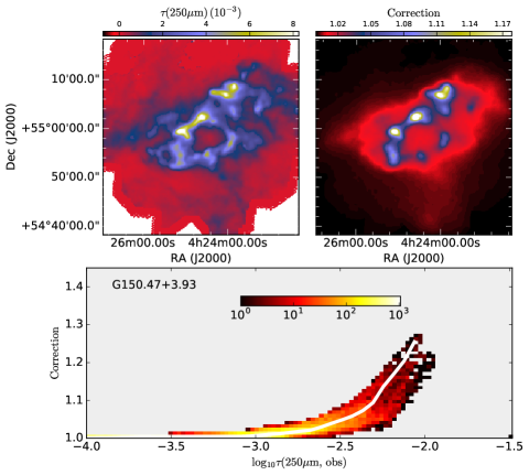
Figure 1: Example of probable column density biases (field G150.47+3.93). The first frame shows the optical depth map derived from observations. Based on RT modelling, and the other frames show the ratio $\xi_{N}$ between the true column density of the model cloud and the column density derived from the model-predicted surface-brightness maps. The bottom frame shows this ratio as a function of the 250 $\mu$m optical depth. The colours correspond to the number of map pixels per parameter area, as indicated by the colour bar. The white curve shows the median relation.

3.3 Clump extraction

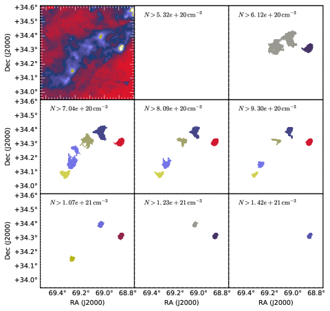
Figure 2: Example of the clump hierarchy. The first frame shows the column density map of the field G167.20-8.69. The other frames show clumps identified on the first seven column density thresholds, different colours denoting different clumps. At the lowest column density threshold, the structure extends beyond the map boundary and therefore is not included in our sample.

We extract from each field the densest structures that are subsequently referred to as clumps. Our sample of fields is very heterogeneous. Based on the estimates derived from SPIRE data, the peak column densities vary by almost two orders of magnitude, from $\sim 5\times 10^{20}$ cm² up to $\sim 5\times 10^{22}$ cm². The resolved linear scales also differ by up to a factor of five because of the different distances. The main purpose of our clump selection is to locate density peaks, most of which may also be relevant to star formation. We also use the clump extraction for a more general characterisation of the density structures. The term “clump” may thus refer to either (gravitationally bound) cores, clumps, or even larger cloud structures.

The two-dimensional (2D) selection is made by thresholding the column density maps, which is a simple and objective way to characterise cloud structure. The column densities are estimated from SPIRE data with MBB fits, assuming a fixed dust opacity spectral index $\beta=1.8$, a dust opacity of $0.1(\nu/1000\,{\rm GHz})^{\beta}\,{\rm cm}^{2}\,{\rm g}^{-1}$, and a total mass of 2.8 atomic mass units per Hydrogen atom; see Juvela et al. (2015a).

We use 38 thresholds that are placed logarithmically between $0.2\,10^{21}$ cm^-2 and $3.5\,10^{22}\,{\rm cm}^{-2}$. Each spatially connected region above a given threshold is counted as a separate clump. Clumps that touch any of the map boundaries (over a distance of five border pixels) or have an area smaller than 0.5 arcmin² (corresponding to the 40$\arcsec$ resolution of the column density maps) are rejected. Thresholding produces clump masks that can be used for any 2D map, including those resulting from the RT models. Figure 2 shows an example of extracted clumps.

Counting all the fields and clumps defined at all 38 column density thresholds, we have 2998 detections. The number is large because of clumps detected at a number of column density thresholds. Selecting in each field the $N({\rm H}_{2})$ threshold that results in the largest number of objects in that field, the median number of clumps is 3 per field. A typical clump is found at a column density level of $N({\rm H}_{2})=8\times 10^{20}$ cm^-2. The number of clumps per column density threshold is not significantly different for fields with distances below and above 250 pc, although more distant fields tend to have a slightly larger fraction of their clumps below $N({\rm H}_{2})=2\times 10^{21}$ cm^-2.

The 3D clumps are defined using volume-density isocontours and are used only in connection with the 3D RT models. These are independent of the 2D clumps but can also be selected to have a similar extent in 2D projection as the 2D clumps. These will be compared later in Sect. 4.6 regarding their estimated stability, the 3D clump analysis making use of the 3D clump density distributions as they appear in the RT models.

3.4 Characterisation of 2D clump structure

We calculate first estimates of clump properties by finding the axis of maximum variance for offsets weighted by column density. We can then proceed to calculate first moments along the major and minor axes, to characterise the elongation (aspect ratio) based on the second moments and asymmetry based on skewness. Similarly, kurtosis characterises the column density profile, separating peaked (high kurtosis) and flat-topped (small kurtosis) shapes.

We also fit 2D models to estimate the size, elongation, and radial profiles of the clumps. We use a Gaussian model with seven parameters: the peak column density, two components of the centre position, the position angle, and the FWHM values along the minor and the major axes. The Gaussian models provide basic estimates of the size and the orientation of the clumps.

To further characterise differences in the shape of the radial column density profiles, we use 2D Plummer functions

$$N(x,y)=N_{0}\left(1+\frac{(x-x_{0})^{2}}{R_{x}^{2}}+\frac{(y-y_{0})^{2}}{R_{y}^{2}}\right)^{-p}+N_{\rm bg},$$ (7)

where the parameters are the peak column density $N_{0}$, the centre coordinates ($x_{0}$, $y_{0}$), and the exponent of the asymptotic powerlaw $p$. The coordinates ($x$, $y$) are measured in a rotated coordinate system, making the position angle an additional free parameter. We can either allow different distance scales through the $R_{x}$ and $R_{y}$ parameters or assume $R_{x}\equiv R_{y}$ To take into account the data resolution, the models are always convolved to the map resolution during the fitting.

Table 3: Fractal dimensions $D_{\rm P}$ of column density maps, confusion noise estimates $S(40\arcsec)$, and the parameters $A$ and $B$ of their dependence on angular separation. The fields are in order of increasing distance.

Field	$D_{\rm P}$	$S(40\arcsec)$ (mJy)	$A^{1}$ (mJy)	$B$
G159.23-34.51	1.25	52.6	78.00	0.54
G155.80-14.24	1.27	43.1	57.74	0.48
G157.08-8.68	1.31	128.3	143.12	0.35
G161.55-9.30	1.28	48.7	64.81	0.54
G149.67+3.56	1.31	47.2	61.85	0.62
G126.63+24.55	1.25	26.1	32.08	0.49
G150.47+3.93	1.34	66.7	98.81	0.55
G163.82-8.44	1.34	62.9	86.98	0.37
G151.45+3.95	1.15	50.8	58.04	0.86
G210.90-36.55	1.19	21.7	25.93	0.72
G167.20-8.69	1.25	30.0	40.13	0.44
G164.71-5.64	1.26	27.0	33.42	0.57
G181.84-18.46	1.21	28.3	42.74	0.69
G154.08+5.23	1.15	57.8	77.68	0.51
G206.33-25.94	1.17	44.8	66.11	0.73
G173.43-5.44	1.26	20.7	26.38	0.52
G188.24-12.97	1.34	25.4	30.83	0.43
G189.51-10.41	1.33	31.1	41.12	0.49
G198.58-9.10	1.23	147.7	163.51	0.33
G212.07-15.21	1.29	25.1	30.83	0.48
G203.42-8.29	1.29	42.8	55.33	0.51
G205.06-6.04	1.32	32.4	41.54	0.53
G247.55-12.27	1.25	26.2	37.33	0.60
G141.25+34.37	1.40	17.7	16.21	0.53
G298.31-13.05	1.16	29.8	42.45	0.64
G300.86-9.00	1.21	30.9	54.12	0.80
G300.61-3.13	1.07	34.2	49.54	0.51
G358.96+36.75	1.05	18.7	24.97	0.99
G4.18+35.79	1.14	39.2	51.71	0.89
G6.03+36.73	1.11	49.6	67.28	0.81
G341.18+6.51	1.05	36.3	59.48	0.71
G344.77+7.58	1.30	37.3	49.40	0.38
G2.83+21.91	1.21	20.3	23.43	0.58
G3.72+21.02	1.26	20.1	24.26	0.50
G0.02+18.02	1.29	28.2	42.03	0.51
G9.45+18.85	1.26	20.0	20.20	0.57
G0.49+11.38	1.17	43.7	66.65	0.68
G3.08+9.38	1.29	34.6	47.19	0.55
G315.88-21.44	1.27	37.6	49.04	0.48
G345.39-3.97	1.27	134.8	177.72	0.37
G1.94+6.07	1.20	36.8	50.45	0.59
G21.26+12.11	1.17	53.2	70.25	0.58
G20.72+7.07	1.28	26.2	32.27	0.41
G26.34+8.65	1.18	31.5	48.08	0.45
G25.86+6.22	1.34	53.9	75.31	0.49
G24.40+4.68	1.24	36.8	50.57	0.48
G93.21+9.55	1.19	50.9	74.29	0.52
G108.28+16.68	1.40	32.3	37.75	0.44
G110.80+14.16	1.29	27.0	32.42	0.50
G110.62-12.49	1.10	24.1	36.99	0.70
G116.08-2.40	1.13	42.6	57.93	0.65
${}^{1}S(\theta)=A\times(\theta/1\arcmin)^{B}$

4 Results

4.1 Characterisation of the fields

Table 3 lists the fractal dimensions $D_{\rm P}$ calculated for the $\tau(250\mu{\rm m})$ maps. The mean value is 1.25, equal to the median value, and with a scatter of $\sigma(D_{\rm P})=0.07$. The use of 250 $\mu$m surface-brightness data (instead of column density) leads to a wider $D_{\rm P}$ distribution with $\sigma(D_{\rm P})=0.13$. This scatter can be affected by noise, which is larger in a single band than in the column densities derived from SED maps. Surface-brightness maps are also more sensitive to dust temperature variations and especially to the presence of warm point sources. The median value is 1.29 and the mean is 1.33. These are higher than the values estimated from column density data but the difference is not very statistically significant ($\sim 1.5\,\sigma$).

The structure functions $S(\theta)$ were calculated for $I_{\nu}(250\mu{\rm m})$ maps by using two symmetrically placed reference positions (see Sect.3.1). To examine the dependence on the angular scale, calculations were done at $40\arcsec$ steps up to a maximum scale of $\theta=600\arcsec$. The value $\theta=40\arcsec$ is close to the resolution limit of the maps, adopting $\theta>2\times D$. At the largest scales, the values become biased, not only because of the finite map size but because the maps are preferentially centred at column density maxima. This selection effect tends to increase $S(\theta)$ when $\theta$ approaches the map radius.

Structure function can be converted to structure noise $N^{\rm str}$ via the relation $N^{\rm str}=\sqrt{S(\theta)}\,\Omega$, where $\Omega$ is the solid angle of the measurement aperture (Kiss et al. 2001). In the upper frame of Fig. 3, the $N^{\rm str}$ values are compared to the analytical expression

$$N^{\rm str}_{\rm HB}(\theta)=0.3\,{\rm mJy}\left(\frac{\lambda}{100\,\mu m}\right)^{2.5}\left(\frac{D}{\rm 1\,m}\right)^{-2.5}\left(\frac{\langle B\rangle}{1\,\rm MJy/sr}\right)^{1.5},$$ (8)

presented by Helou & Beichman (1990). Here $\lambda$ is the wavelength, $D$ the telescope size (assuming diffraction-limited observations that define the angular scale $\theta$), and $\langle B\rangle$ the average surface brightness. For the ratio between the observed and predicted values, $N^{\rm str}(40\arcsec)/N^{\rm str}_{\rm HB}(40\arcsec)$. Compared to Kiss et al. (2001), our scatter is larger but we observe a similar behaviour at low intensities, where the $N^{\rm str}(\theta)$ values tend to rise above the Eq. (8) predictions. Compared to Kiss et al. (2001), our scatter is larger but we observe the same behaviour where at low intensities the $N^{\rm str}(\theta)$ values tend to rise above the prediction of Eq. (8).

The lower frame in Fig. 3 shows the $N^{\rm str}(\theta)$ curves for all fields, with a median relation of $N^{\rm str}(\theta)=48\times(\theta/1\arcmin)^{0.57}$. The Figure highlights some extreme fields. The highest $N^{\rm str}(40\arcsec)$ values are found for G198.58-9.10, G345.39-3.97, and G157.08-8.68. Fields G198.58-9.10 and G157.08-8.68 are indeed filled with significant small-scale structure while for G345.39-3.97 the result can be explained by the compact central region where the surface brightness exceeds 1000 MJy sr^-1. In all three cases, $N^{\rm str}$ increases only slowly with increasing $\theta$. Interestingly, the smallest $N^{\rm str}(40\arcsec)$ values are found for G141.25+34.37 and G358.96+36.75 (LDN 1780), the fields that represented the two extremes of the fractal dimension distribution. This suggests very little dependence between $D_{\rm P}$ and $N^{\rm str}(40\arcsec)$, which is confirmed by a Pearson correlation coefficient $r=$-0.02 for the whole sample. This conclusion does not depend on the scale at which structure noise is evaluated (see Fig. 3b) and remains true if $N^{\rm str}(\theta)$ is estimated using column density instead of surface-brightness data. Both fractal dimensions and structure noise appear to be independent of the linear resolution of the data. The linear correlation coefficient is 0.19 and 0.07 when $D_{\rm P}$ and $N^{\rm str}(40\arcsec)$ are correlated with the field distance, respectively.

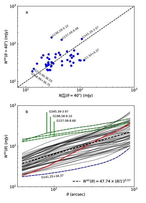
Figure 3: Structure noise $N^{\rm str}(\theta)$ in selected fields. The upper frame shows $N^{\rm str}(\theta=40\arcsec)$ for the 250 $\mu$m surface brightness (blue dots), compared to the surface-brightness dependence of Helou & Beichman (1990) (dashed line). The lower frame shows $N^{\rm str}(\theta)$ in individual fields as a function of the angular scale $\theta$. The black dashed line indicates the median relation. The coloured lines highlight particular fields discussed in the text (G141.25+34.37 as the bottom blue dashed line, G358.96+36.75 as the red solid line, and the fields G345.39-3.97, G198.58-9.10, and G157.08-8.68 as the uppermost dashed green lines).

The PDFs of column density and $250\mu$m surface brightness are shown in Appendix A. PDFs show a range of shapes that are often far from a log-normal distribution. Unlike the fractal dimension or the structure noise, the PDFs also change if the analysis is done with background-subtracted maps. The observations targeted local column density peaks, which directly skews the statistics. The occasional power-law tails towards high column densities are not necessarily a sign of gravitationally bound structures. The PDF plots are affected by the limited size of the fields and often reflect the morphology of individual structures or even a single clump. For example, the field G198.58-9.10 shows a well-defined power-law tail, which is even more pronounced in column density than in surface brightness. The cloud has a high-contrast boundary that is a clear sign of external forcing, possibly by the nearby O star $\lambda$ Orionis or by previous generations of high-mass stars. Such structures have a qualitatively similar effect on the PDF shape, irrespective of gravitational stability of the region. The field G141.25+34.37 is again an outlier, showing a very distinct powerlaw tail towards smaller column densities. In the 250 $\mu$m data, the PDF extends with a similar slope far below the range shown in Fig. 20, which simply reflects the density profile of this diffuse cloud.

The log-normal function often results in a poor fit. To quantify the asymmetry (e.g. in the case of a high-column density tail), we use the skewness and a quantity calculated from the percentile values, $[P(99\%)-P(50\%)]/[P(50\%)-P(10\%)]$. The correlation coefficients between these quantities and the average field column density, the cloud distance, and the Galactic latitude were all small, with $r<0.15$.

To characterise the mass distribution in the fields, we examine the column density profiles around the highest column density peak of each field. The curves in Fig. 4 are obtained by averaging over concentric circles. However, at each distance, the average is evaluated only over those radial directions where the column density is still a monotonously decreasing function of the distance. This reduces the effects of other clumps and local column density peaks, in an attempt to describe the underlying large-scale structure. Beyond $r=$0.1 pc, the radial profiles are well resolved even for the most distant fields. Figure 4 shows that at scales $r=0.1-1$ pc the column density profiles are shallow and typically correspond to $N(r)\propto r^{-1}$ or an even flatter distribution. These describe the profiles of individual regions and are not to be confused with size-mass relations of samples of distinct sources. In the latter, the typical relation $M\sim r^{2}$ simply corresponds to a constant average column density (Larson 1981; Friesen et al. 2016). Mueller et al. (2002) examined the radial profiles for a sample of massive star-forming clouds. On average these corresponded to $M(r)\sim r^{1.2}$. Kauffmann et al. (2010) found a similar relation $M(r)\sim r^{1.27}$ for cluster-forming clouds (see also Beuther et al. 2002; Zinchenko et al. 2005; Schneider et al. 2015b; Lin et al. 2016). These results suggest a column density relation $N(r)\sim r^{-0.8}$. The results of Shirley et al. (2000) on a sample of low-mass star-forming cores gave an average relation of $N(r)\sim r^{-1.1}$. That result is dependent on assumptions of radial dust temperature profiles and also partly relates to scales below our resolution. However, our $N(r)$ profiles in Fig. 4 are compatible with the above-quoted $N(r)\sim r^{-p}$ relations, with some preference for values $p<1$.

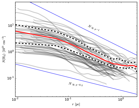
Figure 4: Average column density profiles as a function of the distance from the highest column density peak in each field (grey lines). The thick red line shows the mean column density profile and the dashed lines the average profiles separately for fields with peak column density below or above $5\times 10^{21}$ cm^-2. For comparison, the solid blue lines show the $r^{-1.0}$ and $r^{-0.5}$ relations.

4.2 Basic statistics of the clumps

Clumps are identified through column density thresholding as explained in Sect. 3.3. After subtracting a threshold column density, we determine for each clump the main axis as the direction of maximum column-density-weighted standard deviation of pixel positions. Skewness and kurtosis are calculated for this axis and for the perpendicular direction. In Fig. 5, we have excluded clumps smaller than 2 arcmin² and further divided the clumps to three column density categories. The overall median elongation is 1.5 and the values cover a broad range of values but, surprisingly, are not significantly different for different column density intervals. Even high-density clumps exhibit a wide range of asymmetries, up to a skewness of $\sim$0.8. The third frame of Fig. 5 shows the distribution of kurtosis, or more precisely the excess kurtosis, which is defined to be zero for the normal distribution. Negative values are suggestive of flat-topped structures. Instead of very peaked isolated clumps, the largest positive values are caused by compact structures seen on top of extended diffuse emission. Partly for the same reason, the only significant correlation is observed between clump area and kurtosis. This becomes particularly significant for the subsample of high-density clumps.

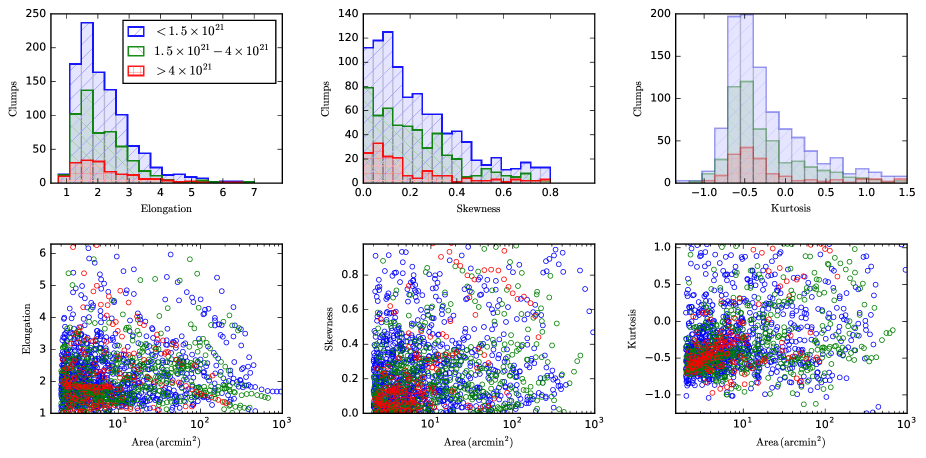
Figure 5: Basic statistics for selected clumps. The colours blue, green, and red correspond to clumps with mean column density $N({\rm H}_{2})<2.1\times 10^{21}$ cm^-2, $N({\rm H}_{2})=2.1-5.0\times 10^{21}$ cm^-2, and $N({\rm H}_{2})>5.0\times 10^{21}$ cm^-2, respectively. In the top row, skewness and excess kurtosis are calculated for the minor axis direction.

The aspect ratios and position angles of the clumps were also estimated by using the fits of 2D Gaussians. Compared to direct dispersion measurements, these respond differently to the presence of secondary peaks or extended, low-column density pedestals under dense clumps. We exclude from the fitted sample clumps that are smaller than 2 arcmin² or for which the relative root mean square (rms) relative error of the fit exceeds 10% (a minor fraction of all clumps). Figure 6 shows the aspect ratios (defined as the ratio of the FWHM values along the major and minor axes) for three column density, clump size, and distance intervals. The statistics are again not strongly dependent on any of these parameters. Symmetric clumps are slightly more likely to be small in size and have high column densities, but this is partly a bias resulting from the finite data resolution. In Fig. 6, the lower frames show corresponding distributions where, for each column density peak, we include only one clump with an area of 10.0 arcmin². The elimination of very extended clumps and clumps near the resolution limit does not have a clear effect on the statistics. Compared to Fig. 5a, the axis ratio (elongation) of Gaussian fits peaks closer to the value of one. This is probably in part a property of the methods used, Fig. 5 being more easily affected by the diffuse background above which more compact structures are seen.

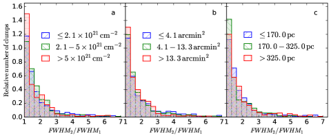
Figure 6: Aspect ratios of the fitted 2D Gaussians. The different histograms correspond to different ranges of column density (frame a), clump area (frame b), and field distance (frame c), as indicated in the frames. The lower frames d-f show the same data for a subset of clumps with areas of 10 arcmin².

4.3 Structure orientation

The results of Sect. 4.2 suggest that in some fields the clump orientations may be correlated. As an example, Fig. 7 shows the orientations of some 10 arcmin² clumps in the field G173.43-5.44. The directions of maximum variance are similar to each other, the result being slightly less clear for major axis directions of Gaussian fits.

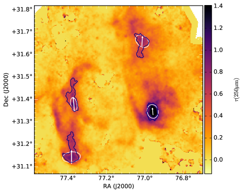
Figure 7: Clump orientations in the field G173.43-5.44. The black contours correspond to the boundaries of the selected structures. The arrows show the direction of maximum variance, with positive skewness along the arrow direction, and the ellipses show the orientation of the fitted 2D Gaussians.

We selected the fields with more than one clump. Clumps were defined using column density thresholds that resulted in clump areas $\sim$10 arcmin². We calculated the quantities $|\theta_{i}-\langle\theta\rangle|$ for each field, measuring the position angle difference between individual clumps and their median. The average values of the individual fields are further grouped to samples with $n=$2, 3, 4, or 5 clumps per field. Above, $\langle\theta\rangle$ refers not to the average but to the median value. Furthermore, when $n$ is an even number, we select as $\langle\theta\rangle$ the value for the index $n/2$ (rather than calculating the average of two elements in the vector).

Figure 8 compares the observed position angle differences to the values expected for a completely random angle distribution. In the fields with just two clumps, the relative orientations of the clumps are significantly correlated. This sample consists of 14 fields. If the angles in those fields were random, the probability for their average of $\langle\theta-\langle\theta\rangle\rangle$ to be below or equal to observed value of 15% is 1.8% (estimated with Monte Carlo simulations). For fields with three or more clumps, the results are compatible with a random distribution. Many of these fields are at relatively large distances and thus have a large physical separation between the clumps. The median distances in the four groups $n=$2-5 are 165, 245, 375, and 200 pc, respectively.

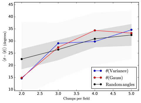
Figure 8: Average difference of the position angles of individual clumps and the average of all clumps in a field. The relation is plotted as a function of the number of clumps in the field, using the directions of maximum variance (blue curve) or the main axis of the fitted 2D Gaussians (red curves). The black curve shows the expected relation for a completely random distribution of position angles. The shaded region corresponds to 68% interval for a single field and the dark shaded region to the 68% interval for the average, taking into account the number of fields with the given number of clumps.

We next compare the clump orientations to the large-scale anisotropy of the column density structures over the entire field. Figure 9 summarises the results. The histograms show the position angle distributions determined with the TM method (see Sect. 3.1). To enable the examination of small spatial scales, the method is applied to the 250 $\mu$m surface-brightness maps with the original $18\arcsec$ resolution. The blue histograms correspond to structures extracted at the ${\rm FWHM}\sim 0.6\arcmin$ scale, using the normalisation that makes the method insensitive to the absolute pixel values. The histogram shows the distribution of the position angles for 10% of positions with the highest significance (see Sect. 3.1). The red histogram is the corresponding distribution of position angles extracted at the larger scale of ${\rm FWHM}=5.0\arcmin$. These correspond to the positions with 20% of the highest significance values, the calculations including the weighting by the local column density. For examples of the TM extractions, see Fig. 7.

In Fig. 9, the circles indicate the position angles (the direction of maximum dispersion) of clumps extracted at different column density levels (see Sect. 3.3). The size of the symbols is related to the clump area and the lines connect each clump to its parent/child clumps at the next lower/higher column density level. Thus, Fig. 9 shows the change of structure orientations as function of both scale and column density.

Clump orientation is often similar to the directions probed by the red histograms, the preferred large-scale orientation of the high-column-density structures. This is often natural because the clumps themselves form a part of the high-column-density structures. Clump orientation carries memory of the orientation of the parent structures, often from column density levels lower by an order of magnitude. We examined this separately for those clumps that include the main column density peak of each field. Comparing the position angles of the clumps defined by the lowest- and the highest-column-density contours, the average value of $\langle\theta-\langle\theta\rangle\rangle$ over all fields is 17.2$\degr$. Comparison to Fig. 8 (for $n$=2) shows that this is still significantly smaller than expected for random angles. There are also exceptions and at the highest column densities the orientation may rotate by up to full 90 degrees (e.g. G345.39-3.97). Significant changes of the orientation are observed also for example in G4.18+35.79, G6.03+36.73, and G167.20-20.89. Even in these cases, the position angles can be strongly correlated between lower column density thresholds.

The Musca filament G300.86-9.00 is an example that shows a clear division between the small- and large-scale structures. The main structure has a position angle of $\theta\sim 30$ degrees and small-scale, lower-column-density striations are preferentially perpendicular to the main filament (Planck Collaboration et al. 2016a; Juvela 2016; Cox et al. 2016). At high column densities, the field contains two main clumps that share the general orientation of the main filament, which here, in fact, is mainly composed of those two clumps. At the highest column densities, their position angles shift with respect to the axis of the main filament. Similar dichotomy is observed, for example, in G210.90-39.55, although this is a more complex object that contains subregions with different preferred structure orientations (Malinen et al. 2016). The same caveat applies to all data. Fields may locally have a more ordered structure than suggested by Fig. 9.

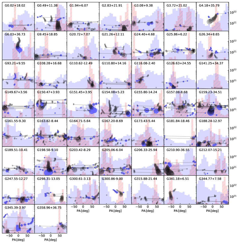
Figure 9: Orientation of structures in the 51 analysed fields. The histograms show the distribution of position angles from the TM analysis with ${\rm FWHM}=0.6\arcmin$ (blue histogram) and ${\rm FWHM}=5.0\arcmin$ (red hatched histograms). The histogram normalisation is arbitrary. The circles show the position angles of the clumps at different column density thresholds (right hand axis, in units of H₂ column density cm^-2). The black and blue symbols are partly transparent and correspond, respectively, to clumps with aspect ratios above and below the value of 1.5. Lines connect clumps to the parent clumps at lower column density levels. The radius of the plotted symbols is proportional to the clump area raised to the power of 2/3.

The TM results can also be investigated in terms of the position angle correlations as a function of the spatial separation or the scale $F$ used in the TM analysis. The differences between structures identified at the scales of 0.6$\arcmin$ and 5$\arcmin$ is visible in Fig. 9. We quantify this further in Fig. 10. The Figure shows the quantity $\langle H(0.6\arcmin)\cdot H(5\arcmin)\rangle$ for each field, where $H$ corresponds to the histograms of Fig. 9 that have been normalised by dividing by the histogram area and by subtracting the mean histogram value. Thus, the plotted quantity is positive if the 0.6$\arcmin$ and 5$\arcmin$ histograms have a similar structure and negative if the distributions are anticorrelated. The significance of the values was estimated with Monte Carlo simulations of 1000 arcmin² maps. The map size is relevant because it limits the number of independent samples, especially at the 5$\arcmin$ resolution. The simulated maps have Gaussian fluctuations, which follow a $k^{-2}$ power spectrum as the function of the spatial scale $k$, have an average surface brightness of 50 MJy sr^-1, and include white noise with a standard deviation $\sigma=0.5$ MJy sr^-1. The 10–90% and 5–95% confidence limits were determined from the analysis of 1000 simulated maps. However, the resulting confidence limits should be considered only as rough estimates, because of the varying size and surface-brightness level of the observed maps. According to Fig. 10, there are only three fields with a significant (at the 5% significance level) positive correlation between the small-scale and large-scale structures. The Musca field G300.86-9.00 remains the only one with a significant negative correlation. As an example, Appendix D shows the extracted structures in the fields G181.84-18.46 and G300.86-9.00.

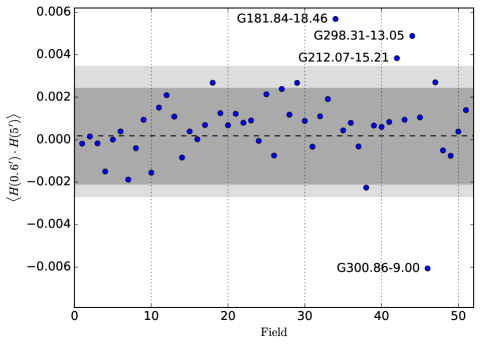
Figure 10: Correlations between 0.6$\arcmin$ and 5$\arcmin$ structures in TM position angle histograms of Fig. 9, $\langle H(0.6\arcmin\cdot 5\arcmin)\rangle$. The grey bands correspond to 10-90% and 5-95% percentile limits and the dashed line to the median value derived from Monte Carlo simulations of fields with random structure orientations. The fields are in order of increasing Galactic longitude.

In principle, TM results could be used to investigate the spatial correlations of the column density anisotropies as a function of the angular separation. This analysis is complicated by the fact that TM only provides position angle estimates for a subset of all map pixels. Thus, the correlations also depend on criteria used to select structures for which the elongation is considered to be significant. Nevertheless, Appendix E shows some results on the angular dispersion functions. G300.86-9.00 is again a special case and has a particularly small dispersion of position angles. At the opposite end can be found fields like G345.39-3.97, which was already found to have one of the largest structure noise values (see Fig. 3).

4.4 Radiative transfer models

RT models are used to investigate the uncertainty of the column density estimates and, for example, variations of the radiation field intensity. In this Section, we describe the main results of the RT models, before using these in the analysis of the radial profiles (Sect. 4.5) and the stability (Sect. 4.6) of the clumps.

4.4.1 The default model

In the default RT models the dust properties are kept fixed and only the model column density and the intensity of the external radiation field are optimised. Dust parameters are characterised by the opacity and spectral index values listed in Table 2.

Observations are fitted by adjusting the radiation field intensity and column density. The models are constructed so that they reproduce the 350 $\mu$m surface brightness and the average surface brightness ratio between 250 $\mu$m and 500 $\mu$m (in practice, to an accuracy of 1% or better). At 250 $\mu$m and 500 $\mu$m, the residuals vary from position to position but are typically a few percent and thus smaller than the observational uncertainty. Nevertheless, visual inspection shows several cases where the residuals are significant. Some examples are given in Appendix B. First, the assumption of an isotropic radiation field is not always fulfilled. This can be caused by local heating source, the effect usually extending over a few Herschel beams. However, in the field G110.62-12.49, a star (not visible in submm maps) is located between the two main clumps and the effect is more widespread (see Fig. 2). The anisotropy may also be in the external field. The best examples are G358.96+36.75, G4.18+35.79, and G6.03+36.73, where the asymmetry is caused by the direction of the Galactic plane and the contribution of the high-mass stars of the Sco-Cen OB association (Ridderstad et al. 2006). The effect is particularly pronounced in the case of the high-column-density fields G358.96+36.75 and G4.18+35.79. Figure 3 shows data for G4.18+35.79 where the maximum 250 $\mu$m residuals are up to +15% within the core and down to -20% on its shadow side. The residuals clearly show the presence of a NW-SE gradient. The colour temperature map shows two cold subclumps. The northern one is significantly colder than predicted by the RT model while the southern one is warmer. Further quantitative analysis would require modelling that explicitly includes the field anisotropy. However, apart from the examples listed above, this is not a significant factor and is not taken into account in this paper.

A potentially equally important effect is observed in some fields where the densest clumps appear to reach much lower temperatures than predicted by the models. As a result, the 250 $\mu$m residuals are negative with magnitudes up to $\sim 10$%. One example is shown in Fig. 4. This is a field with complex structure where also the dense clumps (identifiable in the colour temperature map) do not entirely coincide with the 250 $\mu$m peaks. The RT model overestimates the temperature of the main clumps and, because the radiation field is adjusted based on average emission over a large area, the model produces too little short wavelength emission for the most diffuse material.

These discrepancies are interesting because they could indicate a change in dust properties, an enhanced long wavelength emission that leads to lower temperature (or a change in the opacity spectral index). However, there are other possible explanations. First, the ISRF level is adjusted according to the average spectrum over a large area. In spite of background subtraction, this may include diffuse material that may be subjected to a stronger radiation. The models assume a cubic volume that, depending on the angular size and distance of the field, can extend up to $\sim$6 pc. The actual emission may originate over a wide range of distances and in even completely different radiation field environments. Second, the finite resolution of the models (including the LOS density profile) may underestimate the value of the peak column density. If the 350 $\mu$m surface brightness saturates because of an extreme density, a higher column density may actually result in lower surface brightness (see Juvela et al. 2013).

4.4.2 Variations of the basic models

In addition to the default models of Sect. 4.4.1 (model version $D$), we carried out model fits with alternative sets of assumptions that are listed in Table 2. The versions $P$ and $W$ are directly aimed at improving the fits of the dense clumps by, respectively, concentrating on the higher-column-density peaks or by including the LOS cloud size as additional free parameters. A decrease (increase) of the external extinction layer $\Delta A_{\rm V}$ could similarly help the fits by increasing (decreasing) the temperature contrast between low- and high-density regions. The versions $K$ and $TD$ are the same as $D$ except for the use of different dust properties. In the $K$ version we use dust with a higher sub-millimetre opacity and a higher opacity spectral index (see Sect. 3.2.1). In the $TD$ version the dust properties transform smoothly from $D$ to $K$ dust as the density increase from $n({\rm H_{2}})\sim 10^{3}$ cm^-3 to $n({\rm H_{2}})\sim 10^{4}$ cm^-3. In practice, we modify the abundances of the two dust components so that their sum remains constant and the relative abundance of the default ($D$) dust is $0.5\times(1+\tanh[2\,\log(n/1000\,{\rm cm}^{-3})])$.

Figure 11 gives a summary of the relative quality of all fits. The only clear systematic effect is the somewhat higher average $\chi^{2}$ value of $\Delta A_{\rm V}=-1$ mag fits. The small differences reflect the fact that most map pixels are located at moderate column densities where the changes are not expected to have a strong effect on the fit quality. The version $P$ fits (not shown) concentrate on the small regions with high column densities and therefore also show somewhat elevated $\chi^{2}$ values (similar to those of version $\Delta A_{\rm V}=-1$ mag) and give a better fit only within the densest regions. The $\chi^{2}$ outliers G126.63+24.55 and G315.88-21.44 both have large areas with column density below $N({\rm H}_{2})=2\times 10^{20}$ (before background subtraction). In these cases, the errors appear to be dominated by random noise rather than systematic effects.

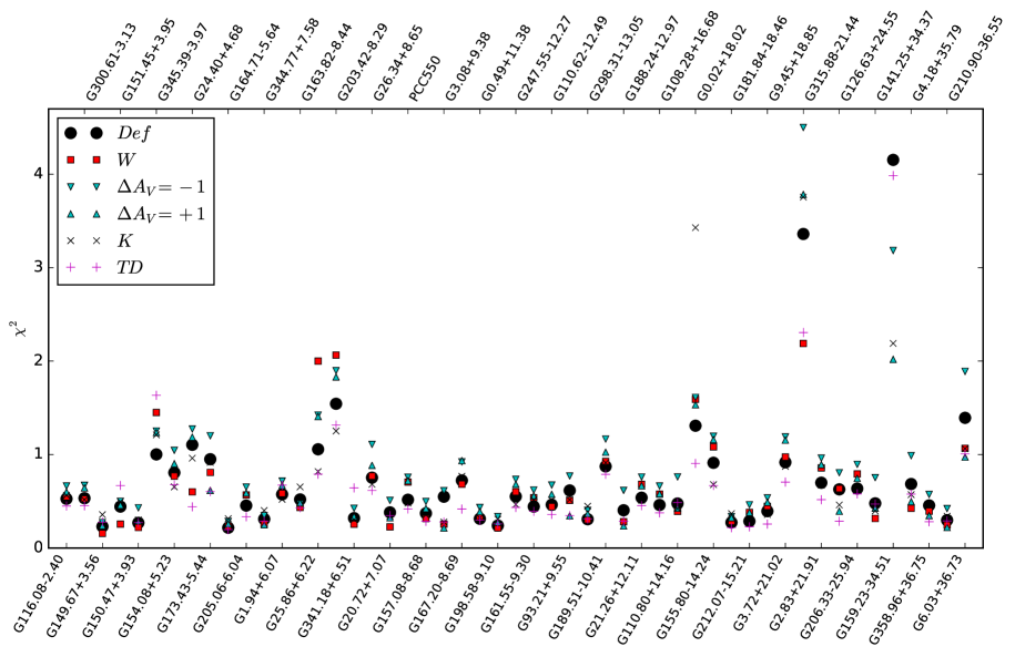
Figure 11: $\chi^{2}$ values of the RT model fits. The reduced $\chi^{2}$ values are calculated over the 250, 350, and 500 $\mu$m maps assuming an observational uncertainty of 7%. The fields are arranged in the order of increasing $|b|$. The legend refers to the model variations listed in Table 2.

Although the $\chi^{2}$ values are similar, different assumptions lead to significantly different parameter values. Figure 12 shows the estimated strength of the radiation field $k_{\rm ISRF}$. As described in Sect. 3.2.2, $k_{\rm ISRF}$=1 corresponds to a case where the incoming radiation is assumed to be attenuated by an external layer that corresponds to the amount of material in the reference area (used for background subtraction). The case $\Delta A_{\rm V}=-1$ mag is included in the plot as the one resulting in the lowest $k_{\rm ISRF}$ values. The magnitude of this drop is not trivial to predict because a change in $\Delta A_{\rm V}$ also changes the shape of the incoming spectrum. The plot shows the clear increase of $k_{\rm ISRF}$ in the case of a higher sub-millimetre opacity.

The parameter $k_{\rm ISRF}$ does not show any systematic behaviour as a function of Galactic longitude. The intensity tends to decrease with increasing Galactic latitude, the overall trend in Fig. 12 being significant at a $\sim$2.5 $\sigma$ level. There is no similar dependence on distance. The correlation between $k_{\rm ISRF}$ and the Galactic height is even slightly (but not significant) negative.

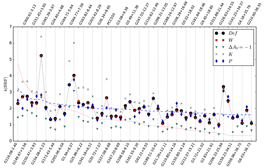
Figure 12: Strength of the external radiation field, $k_{\rm ISRF}$, derived under various assumptions of the RT models. The fields are in increasing order of $|b|$. The blue dashed line shows the fitted least squares line $k_{\rm ISRF}=(1.49\pm 0.24)+(0.074\pm 0.029)\times csc(|b|)$. For comparison, the red dotted line indicates a pure cosecant law (with an arbitrary scaling).

4.5 Clump radial density profiles

We examine in more detail the radial density structure of a subset of clumps. The sample is selected by taking the clumps with areas close to 10 arcmin². The value is well above the effective beam size but still corresponds to relatively compact objects. Because the selection is based on angular size, the physical sizes of the clumps vary depending on the distance. The importance of this fact is examined at the end of this Section. To enable better fitting of the 2D surfaces mentioned in Sect. 3.4, we exclude clumps that have strong secondary peaks. This leaves a sample of 85 clumps.

The clumps were fitted with 2D Gaussians and 2D Plummer functions. The statistics of all fit parameters are shown in Appendix C. Even the simpler Gaussian model gives relatively good fits with residuals below 10%. The Plummer fits suffer from a large number of free parameters (and degeneracy between $R$ and $p$ parameters). In particular, the asymptotic power law exponent $p$ does not appear to be at all well constrained. Figure 13 shows the parameters $p$ and $R$ of the Plummer fits, assuming the same value of $p$ for both the minor and major axes. The flat radius $R$ is concentrated at values below 0.1 pc but, depending on the distance of the clump, this scale is only marginally resolved. The largest values near $R=$0.2 pc are well below the limit set by the selected 10 arcmin² clump sizes. The values of the exponent $p$ are spread between zero and $p=5$, the maximum value allowed in the fits. Only the lack of combinations of small $p$ and small $R$ values is related to the data resolution. In total, at the scale of 10 arcmin², the fit parameters scatter over a large parameter range and, as far as characterised by the Plummer fits, the clump shapes do not show any clear trends.

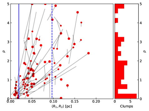
Figure 13: Results of 2D Plummer function fits. The circles correspond to the parameters $p$ that are plotted against the geometrical mean of the flat radii $R_{1}$ and $R_{2}$, which correspond to the clump major axis and minor axis directions. The solid lines are drawn from the plotted circles to the parameter combination that is obtained when clumps are selected at a 15% higher-column-density threshold. The solid and dashed vertical lines correspond to 40$\arcsec$ at 100 pc and 500 pc distances, respectively. The right panel shows the distribution of $p$ values ($0\leq p\leq 5$ only) corresponding to the red symbols of the first frame.

Because of the inconclusive results of the 2D fits, we made fits also to azimuthally averaged column density profiles. Appendix F shows the column density maps and the radial optical depth profiles, also including the corrections derived from the RT models. After subtracting the threshold column density, the median FWHM of the clumps is 0.075 pc. This differs only slightly between clumps below and above the median column density, with 0.092 pc and 0.071 pc, respectively. The clumps with one or more YSO candidates within their perimeter are more compact with FWHM=0.037 pc compared to FWHM=0.077 pc for the remaining sources (median values).

The clump profiles were fitted with powerlaws and with one-dimensional (1D) Plummer functions, the 1D versions of Eq. (7). Both fits include a constant background as one of the free parameters. In the Plummer fits, the beam convolution is also explicitly taken into account. For powerlaw profile, $Ar^{-p}+B$, to reduce the effects of the finite beam, we simply limit the fits to angular distances larger than 30$\arcsec$.

Figure. 14 shows the distribution of the powerlaw exponents. The plot is limited to a maximum value of $p=$5 (one powerlaw fit resulted in a value above this limit). The Plummer fits were directly constrained to values $p<5$. There is again a large scatter in the Plummer parameters. For the pure powerlaw fits, the exponent values are more concentrated below $2$ and there is a clear local maximum around 1. The median value is +0.85 for the whole sample but one in four clumps has a powerlaw exponent smaller than 0.2. Appendix F shows that some of the very low $p$ values are associated with double-peaked column density structures or poorly resolved clumps inside the 30$\arcsec$ radius. However, these do not explain all the low $p$ values and generally the low $p$ values are not associated with the particularly large fit residuals. There is some tendency for the profiles to be steeper in regions of high column density. However, the correlation with the background value is only marginal, both for the exponents of the pure powerlaw fits ($r=$0.15) and for the Plummer $p$ parameter ($r=$0.30 for the sample with fitted values $0<p<5$)

Because the distances of the fields range from $d$=110 pc to $d$=500 pc, the fits apply to different physical scales. At $d$=110 pc the fitted radial range can be 0.016–0.08 pc while for $d$=500 pc it could be 0.07–0.36 pc. Here the calculated upper limits correspond to a radial distance of 2.5$\arcmin$. Nevertheless, the correlations between the fit parameters and the distance are weak. The linear correlation coefficient is -0.02 in the case of the Plummer $p$ parameter and +0.27 in the case of the powerlaw exponent. Even the latter is only marginally significant, which suggests similarity in the typical clump profiles across the $\sim$0.1 pc scale.

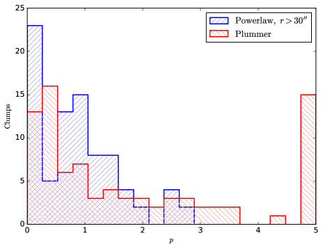
Figure 14: Distribution of the exponents of the azimuthally averaged optical depth profiles. The pure powerlaw fits (blue histogram) are to data with $r>30\arcsec$. The Plummer fits (red histogram for the parameter $p$) are to data $r<0.15$ pc.

4.6 Clump stability

We estimate the clump stability using both the column densities derived from observations and the 3D density distributions of the RT models. We do not have uniform high-resolution line observations and thus no precise knowledge of the thermal and turbulent support or the external pressure. We make the assumptions that the gas kinetic temperature is 10 K inside the objects and 15 K in their envelopes. Following the compilation of observations in Kauffmann et al. (2013), we adopt a 1D, non-thermal velocity dispersion of $\sigma_{1D,NT}$ = 0.7 km s^-1 ($R_{\rm eff}$/1pc)^0.4, where $R_{\rm eff}$ is the radius of a circle with an area equal to that of the clump. We assume that the velocity dispersion within the source is smaller by 30%, as justified below.

Line observations do exist for some of the selected clumps and for some GCC fields that are not part of the present sample. The observations are not sufficiently complete for the virial analysis to be directly based on them. However, we can compare the Kauffmann et al. (2013) relation with these data. The relation is fully consistent with mean behaviour of the ¹³CO data in Fehér et al. (2017), although observations show a 40% dispersion relative to the relation. Saajasto et al. (2017) investigated the $Herschel$ field G82.65-2.00 that is not included in the present paper because of its 650 pc distance. In that field, which contains a star-forming and strongly fragmented filamentary cloud, the large-scale velocity dispersion was found to be almost independent of the linear scale. However, based on the ¹³CO data, the 1D velocity dispersion of the main clumps was about 0.6 km s^-1. With the assumed cloud distance, the sizes of the clumps are about one parsec and the values are again consistent with the Kauffmann et al. relation. Parikka et al. (2015) reported line widths that were based on C¹⁸O observations of compact objects with sizes below 0.5 pc. The median line width was some 30% below the Kauffmann et al. relation. We adopt $\sigma_{\rm 1D}$ values that are 30% below the (Kauffmann et al. 2013) relation as an approximation of the internal velocity dispersion of the clumps, as it would be seen in C¹⁸O observations. This is, of course, valid only statistically and should not be used to infer the gravitational stability of any individual object.

We calculate the virial parameter $\alpha_{2D}=M_{\rm vir}/M_{\rm 2D}$ using the clump masses integrated from column density maps, after subtracting the background level that is estimated as the average value within a one-arcmin-wide boundary just outside the clump perimeter. The virial mass is obtained from

$$M_{\rm vir}=168.5\,R_{\rm eff}\,\sigma_{\rm 1D}^{2}\,8\ln{2},$$ (9)

(MacLaren et al. 1988), which includes the assumption of an $r^{-1.5}$ density profile. In this form, $\sigma_{\rm 1D}$ includes both the thermal and non-thermal velocity dispersions, which are added together in squares. In the following, the $\alpha_{\rm 2D}$ parameters are calculated by directly using the column densities derived from SED fits, without the RT-derived corrections.

Alternatively, the clump stability can be estimated using the 3D models and the direct balance of gravitational, kinetic, and external pressure energies. The 3D models take into account the effects that temperature gradients have on the observed surface brightness and may therefore lead to different estimates of the gravitational energy. The 3D clumps are defined by a density isocontour that has projected areas similar to the selected 2D clumps. For comparison, we also consider smaller clumps that are defined by density isocontours with 20%, 40%, and 60% higher column density values (objects smaller than 1.1 arcmin² are excluded). We consider the gravitational potential energy $\Omega_{\rm G}$, the internal (kinetic) energy $\Omega_{\rm K}=3PV$, and the term $\Omega_{\rm P}$ that is related to the external pressure. The value of $\Omega_{\rm G}$ is calculated explicitly, using the density distribution of the 3D model. Because of the assumptions on $\sigma_{1D,NT}$ (see the beginning of this Section), the pressure $P=\rho\sigma_{\rm 1D}^{2}$ only depends on the scale at which it is estimated, the gas kinetic temperature, and the density threshold $\rho$. Therefore, $\Omega_{\rm K}$ is calculated with $\sigma_{\rm 1D}$ values that are estimated for $R_{\rm eff}$ and include thermal motions at the assumed kinetic temperature of 10 K. The energy related to the external pressure is $\Omega_{P}=-3P_{\rm ext}V$, where the volume is the actual volume of the 3D clump and the pressure is again estimated at the scale $R_{\rm eff}$, assuming a kinetic temperature of 15 K. We do not have observations of different molecules that could be interpreted as direct measurements of the velocity dispersion inside the clumps and at their boundary (cf. Pattle et al. 2015). By using the same $\sigma_{1D,NT}$ values for both $\Omega_{\rm K}$ and $\Omega_{\rm P}$ (apart from the different kinetic temperature), we may underestimate the importance of the outer pressure, provided that turbulence is stronger outside the clump.

We use the same sample as in Sect. 4.3, the clumps with projected area of approximately 10 arcmin². Figure 15 shows the 2D and 3D clump masses as a function of the effective radius, $R_{\rm eff}$, which in the case of 3D models also corresponds to the projected area in the POS. The results correspond to the default assumption of the dust properties with $\tau(250\mu{\rm m})/\tau(J)=1.0\times 10^{-3}$. The use of a higher emissivity would naturally lead to smaller clump masses and higher values of the virial parameter.

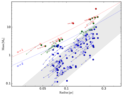
Figure 15: Clump masses as a function of the clump effective radius. The sample consists of 10 arcmin² clumps. The circles denote values derived from the observed column density maps. The crosses are the values from 3D models, smaller symbols corresponding to progressively higher volume density thresholds. The dotted lines correspond to the values $\alpha=1$ and $\alpha=2$ of the virial parameter (3D clumps), with the assumptions listed in the text. The red, green, and blue symbols show the actual values with $\alpha<1$, $1<\alpha<2$, and $\alpha>2$, respectively. The grey band corresponds to an empirical relation of CO clumps (Elmegreen & Falgarone 1996; Pattle et al. 2015).

Figure 16 shows the same 3D data against the different energy components. In this Figure, 25% of the clumps are gravitationally bound and 40% are bound by the external pressure. It is also clear that the selected density threshold has a non-negligible effect on the virial parameter estimates. At a higher density threshold, the $\Omega_{\rm G}/\Omega_{\rm P}$ tend to be smaller while several unbound objects also cross the $-0.5(\Omega_{\rm G}-\Omega_{\rm P})/\Omega_{\rm K}$ boundary. Thus, by selecting a 40% higher density threshold, the fraction of gravitationally bound objects decreases to 21% while the number of pressure-bound clumps increases to 53%. Of course, the behaviour directly depends on several assumptions, including the adopted velocity scaling and gas temperatures.

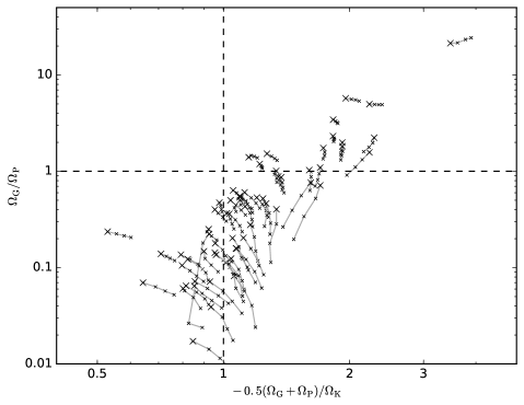
Figure 16: For the sample of 3D clumps in Fig. 15, energy ratios based on the terms $\Omega_{\rm G}$, $\Omega_{\rm P}$, and $\Omega_{\rm K}$. The larger symbols refer to clumps with a projected surface area of 10 arcmin². The smaller symbols, joined by lines, correspond to smaller clumps defined by, in steps of 20%, higher volume density thresholds. The clumps right of the vertical line are bound and the clumps above the horizontal line are dominated by gravity.

According to Fig. 17, there is a clear correlation, at least for the upper envelope of the $\alpha$ values, such that clumps with smaller virial parameters are much more likely to be found in regions of higher column density. At $N_{\rm BG}>5\times 10^{21}$ cm^-2 ($A_{\rm V}>5\,$mag), most of the clumps are almost bound ($\alpha\la 2$). Here the values $N_{\rm BG}$ consist of the immediate surroundings of the clumps. It does not include the global background that for each $Herschel$ field was subtracted when the column densities were estimated from background-subtracted surface-brightness measurements. If those larger-scale backgrounds were included, the correlation of Fig. 17 would remain but also become much less pronounced. This is natural if the background subtraction has removed mainly emission that is unrelated to the clumps and simply originates elsewhere along the line of sight.

Figure 17: Virial parameter $\alpha$ as a function of the estimated background column density $N_{\rm BG}$. The $\alpha$ values estimated from 2D and 3D data are, respectively, shown as blue circles and red triangles. The vertical lines indicate the approximate values (depending on the dust model) of $A_{\rm V}$ equal to 5 and 10 magnitudes. Horizontal lines are drawn at $\alpha=1$ and $\alpha=2$.

The virial parameter is not correlated with either skewness or kurtosis of the clumps. The only potential dependence is seen with clump elongation. According to the Gaussian fits, the average elongation (ratio of major and minor axes) is 1.63 for the $\alpha>2$ clumps and 1.38 for the $\alpha<2$ clumps. Thus, more bound clumps also appear to be more spherical. However, considering the standard deviations and counts within the two samples, the difference is significant only at 1.8-$\sigma$ level.

The estimates of clump mass and of $M_{\rm vir}$ are affected by several sources of uncertainty. The separation of the clumps from the background may cause systematic effects such as those associated with limb brightening at short FIR wavelengths (Men’shchikov 2016). The average column density in clump apertures is only $\sim$40% higher than in the reference annuli, which suggest that the uncertainties associated with background fluctuations can be significant. An order-of-magnitude estimate can be derived using Eq. (8). Assuming a dust spectrum of $B_{\nu}(T=15{\rm K})\nu^{1.8}$, the average clump background level of 55 MJy sr^-1 corresponds to a confusion noise of $\sim$10 MJy sr^-1 at the scale of 2$\arcmin$. This is more than 40% of the average clump signal relative to background. Of course, this is error only so far as the fluctuation is not associated with the main object. Because clumps are defined with column density isocontours, a positive fluctuation at the clump location is likely to increase both the mass and (via $R_{\rm eff}$) $M_{\rm vir}$ estimates, with a smaller effect on the virial parameter. The effect of the threshold used in the clump definition is directly visible in Figs. 15-16. The unknown LOS extent of the clumps acts as a similar error source, especially for $\alpha_{\rm 3D}$. The difference between a sphere and a bi-axial ellipsoid with an aspect ratio of 1:2 is 30% in gravitational energy. The distance estimates $d$ have a typical accuracy of 30% (Montillaud et al. 2015) but they affect the mass estimates in squares. $M_{\rm vir}$ depends directly on $R_{\rm eff}$ while $\sigma_{\rm 1D}$ is in our case proportional to $R_{\rm eff}^{0.8}$. Thus in our calculations the distance dependence of the virial parameter $\alpha$ is only $d^{-0.2}$. The masses were derived for fixed values of dust opacity $\kappa$ and opacity spectral index $\beta$ (Sect. 3.3). A $\beta$ uncertainty of $\sigma(\beta)=0.2$ corresponds to 30% uncertainty in mass while the effect of the $\kappa$ uncertainty is potentially even larger (Juvela et al. 2015b). These can increase the scatter and introduce bias in Figs. 15-17. $M_{\rm vir}$ is further affected by the uncertainty of the $\sigma_{\rm 1D}$ parameter. If C¹⁸O line widths have a 30% scatter (normal distribution) around the adopted analytical relation, the resulting noise in $M_{\rm vir}$ would be close to 60% (standard deviation). If C¹⁸O does not accurately measure the relevant velocity dispersion, the $M_{\rm vir}$ estimates can be correspondingly further biased.

5 Discussion

We have investigated 51 fields that are within 500 pc distances and were originally targeted by $Herschel$ observations because they contain $Planck$ detections of cold clumps. Low dust temperatures imply large column densities that are able to produce large temperature gradients, especially because PGCC, the catalogue of $Planck$ detections, is based on the relative temperature of the clumps and their environment. Thus, PGCC may also contain relatively diffuse sources (sources with small internal temperature gradients) if they happen to be seen against a much warmer background. The term “background” could mean other clouds along the LOS that either are subjected to a stronger radiation field or have different dust properties. However, previous studies of the GCC fields have already confirmed the presence of cold clumps that truly dominate the LOS column density. In this paper, we have tried to further characterise both the global properties of the fields and the individual properties of the selected clumps. This could shed some light on the clump formation as an important intermediate step in the star formation process.

5.1 General properties of fields with Planck cold clumps

We analysed the large-scale properties of the $Herschel$ maps using standard statistical methods. The results show that the fields are in many respects typical of interstellar clouds.

5.1.1 Fractal dimension

The fractal dimensions of the column density maps were $D_{\rm P}=1.25\pm 0.07$. The nearby cloud G358.96+36.75 is one extreme and, with its smooth radial density profile, appears almost non-fractal with $D_{\rm P}=$1.05. The highest values were around 1.4 but these are sometimes found in fields with very low column densities where the values are affected by observational noise and even the extragalactic background. Both act as noise, which tends to increase the $D_{\rm P}$ values (Vogelaar & Wakker 1994; Pant 2013).

To an accuracy of 0.02 units, the median value of $D_{\rm P}$ over all fields remains the same if the calculations are done using contours below or above the median of the original set of column density thresholds. We also estimated $D_{\rm P}$ for the subset of structures with surface area below or above the median structure size. The median value is lower by 0.06 units for the smaller structures and higher by 0.05 units for the larger structures. This could hint at the presence of small, gravity-bound structures of low fractal dimensions. However, because no significant correlation was found with the distances, the dependence seems to be more on the angular rather than the physical scale.

$D_{\rm P}$ values usually reported for interstellar clouds are in the range of 1.2-1.5. Falgarone et al. (1991) obtained $D_{\rm P}$=1.36 from ¹²CO data over a wide range of spatial scales. Sánchez et al. (2005) and Sánchez et al. (2009) derived from CO isotopologues estimates 1.30-1.35 for the Ophiuchus, Perseus, and Orion A clouds. The IRAS 100 $\mu$m data have given similar values with $D_{\rm P}$=1.26 at high latitudes (Bazell & Desert 1988), $D_{\rm P}$=1.4 for the Taurus clouds (Scalo 1990), and a range of values 1.2-1.3 for a sample of nearby molecular clouds (Dickman et al. 1990). As noted by Sánchez et al. (2009), values $D_{\rm P}\sim 1.35$ are more consistent with a 3D fractal dimension $D_{\rm f}\sim 2.6$ than the direct estimates of $D_{\rm P}$+1. Thus, the more recent values reported by Elia et al. (2014) for column density maps of HiGal $Herschel$ fields, $D_{\rm f}$=2.61–2.93, while being slightly higher, are still relatively close to our values. Elia et al. (2014) found that $D_{\rm f}$ decreases with the wavelength of the surface brightness maps. Furthermore, $D_{\rm f}$ calculated from column density was on average more than 0.1 units lower. The difference is similar in our data, the 250 $\mu$m surface brightness data resulting in $D_{\rm P}$ values higher by 0.08 units (see Sect. 4.1). We saw no clear indication that the fractal dimension would depend on the column density. If gravitation produces more spherical dense structures, one could expect $D_{\rm P}$ to decrease with column density. Because we exclude contours close to the resolution limit, scales $<1\arcmin$, we are not probing actual core scales. Thus, the fractal dimensions are relatively constant between the fields, between regions of different column density, and also between small and large linear scales. Although our fields are outside the Galactic plane, there is little difference even from the (Elia et al. 2014) data, which correspond to much longer sightlines through the Galactic plane and thus could be expected to represent a superposition of several clouds.

5.1.2 Structure noise

The structure noise $N^{\rm str}(\theta)$ of the 250 $\mu$m surface brightness (Fig. 3) are consistent, within a factor of $\sim 2$, with the intensity-dependence previously observed in 100 $\mu$m IRAS data (Helou & Beichman 1990; Gautier et al. 1992) and, for example, in selected ISO satellite observations (Kiss et al. 2001). The structure noise appears to probe a generic property of the ISM and the same laws apply to such different types of objects as cirrus clouds and our sample of dense and in some cases actively star-forming clouds. The $N^{\rm str}(\theta)$ values show variations as a function of both the surface brightness and the angular scale. The average angular dependence was found to be $N^{\rm str}(\theta)\sim\theta^{0.57}$ but in individual fields the exponent could be as low as 0.35. For nearby fields, the calculated $N^{\rm str}(\theta)$ is no longer in the same sense a statistical description of the column density fluctuations. When the map is dominated by a single clump, $N^{\rm str}(\theta)$ also mainly describes the radial profile of the clump. As an extreme case, the smooth profile of G358.96+36.75 (LDN 1780) results in a very steep relation with $N^{\rm str}(\theta)\sim\theta^{0.99}$.

5.1.3 Column density PDFs

The column density PDFs of clouds are often described as a combination of a log-normal distribution and a power-law tail at large column densities. These should be connected to key cloud properties; for example, the Mach number and the appearance of gravitationally bound structures, respectively (e.g. Vazquez-Semadeni 1994; Padoan et al. 1997; Kainulainen et al. 2009; Schneider et al. 2013; Ward et al. 2014). We show the column density PDFs of the analysed fields in Appendix A. Although the average PDF is close to the log-normal shape expected of turbulent clouds, the individual fields exhibit a wide range of shapes. Some individual fields are examined further in Appendix G.

Because the 250 $\mu$m surface brightness is usually a good proxy of column density, the differences between surface brightness and column density PDFs are small. When the differences are noticeable, the column density PDF extends to higher values. This is caused by high-column-density structures being colder and thus under-represented in surface brightness data.

Because observations target high-column-density structures, the low-$N$ extent of the PDFs is dependent on the map size and on the low level to which column density observations extend (Ossenkopf-Okada et al. 2016; Alves et al. 2017). Background subtraction makes the distributions wider and, by construction, the PDF will extend to zero column density (-$\infty$ on logarithmic scale). The ambiguity of the background subtraction makes the interpretation of the low-$N$ tail problematic (Schneider et al. 2015b; Ossenkopf-Okada et al. 2016; Alves et al. 2017). On the other hand, the high-$N$ side of the PDFs is, in first approximation, only stretched as the mean column density decreases. The background-subtracted data cover the regions selected for RT modelling (see Table 1). The RT models indicate that the bias in column density values (caused by LOS temperature variations) is typically 10% or less. This is small compared to the full dynamical range and, after the renormalisation with the average column density, the effect is not easily visible in logarithmic plots. However, the correction can sometimes have a significant effect on the high-$N$ tail at $N({\rm H}_{2})>10^{22}{\rm cm}^{-2}$. In G6.03+36.74 the correction makes the PDF tail a true powerlaw that extends down to the resolution limit. This shows that as soon as optical depths are tens of $A_{\rm V}$, the PDF derived from basic SED analysis can be significantly biased.

A tail of the PDF towards high column densities is sometimes taken as an indicator of the presence of dense cores or of a general tendency to star formation. It is likely to be a more complex phenomenon, involving the individual history of the cloud and the potential effects of external forcing, magnetic fields, intermittent turbulence, and feedback from the star-formation process (Kainulainen et al. 2011; Schneider et al. 2013, 2015b; Anathpindika et al. 2017). In our case, the situation is further complicated by the fact that the observations target distinct column density peaks with maps of limited size. Thus, the extracted PDF can reflect the column density profile of a single structure more than the relative statistics of low- and high-column-density objects (see Appendix G). A high-column-density tail is also thus not automatically an indicator of gravitationally bound substructures.

We correlated the skewness and the asymmetry parameter $[P(99\%)-P(50\%)]/[P(50\%)-P(10\%)]$ with several quantities. The linear correlation coefficients with the column density were compatible with zero ($r\sim 0.015$). The surface density of YSO candidates was estimated with the YSO catalogues of both Montillaud et al. (2015) and Marton et al. (2016). The correlations were positive but the correlation coefficients $r\sim 0.1$ are not significant even at the 85% confidence level. If the powerlaw tail is caused by the presence of dense cores, these need to be at least partially resolved. In their study of the Taurus molecular cloud, Pineda et al. (2010) concluded that the powerlaw tail is noticeable at scales below $\sim$0.4 pc. These are in principle well resolved in all our fields but the correlations between PDF asymmetry and distance were negative. This may be the expected behaviour (Alves et al. 2017) but in our study the correlation coefficients ($r=-0.11$ for skewness, $r=-0.06$ for the asymmetry parameter) were not statistically significant.

We do not find significant correlation between power-law tails at high column density and the presence of gravitationally bound structures or star-formation activity (YSOs), as reported in the literature (Kainulainen et al. 2009; Schneider et al. 2015a). However, our study is partly limited by the map sizes. The column density PDFs show a wide range of shapes that often are far from a log-normal distribution. The strongest asymmetries are related to the structure of individual clumps or to dynamical interactions that lead to sharp cloud boundaries.

5.2 Radiative transfer models

We carried out RT modelling of all the fields. This was done to estimate the possible bias of the standard analysis through modified blackbody fits, to probe the systematic effects that result from unknown dust properties and unknown LOS cloud shapes, and to derive estimates of the relative strength of the radiation field. The 3D model clouds were also used to examine the gravitational stability of selected clumps.

We compared the column densities of the optimised models and the values derived from the surface-brightness maps predicted by the models. This allowed us to estimate the bias of the normal SED analysis and to derive multiplicative corrections. One example was shown in Fig. 1, where the error rises to about 20% in the densest part of the field but is much smaller over most of the field. The bias estimates themselves depend on assumptions about the dust and the cloud properties. The bias systematically increases with increasing column density. This trend could be changed only if the observed surface brightness is affected by internal heating sources (Malinen et al. 2011). Our models do not include embedded sources but, according to surface brightness data, their effect is constrained to small areas. The bias can be a significant source of systematic error that should be considered in addition to the (typically larger) uncertainty of the dust properties.

Figure 18 shows the distribution of the estimated maximum bias in each field. The errors are mostly below 20%. In the cloud LDN 183 (field G6.03+36.73) the estimated error is a factor of five. In LDN 183 molecular line data, 8 $\mu$m absorption, and millimetre dust emission are all consistent with a maximum column density in excess of $N({\rm H}_{2})=10^{23}$ cm^-2 (Pagani et al. 2015; Lefèvre et al. 2016). The bias estimate is roughly consistent with the difference between these estimates and the values derived from $Herschel$ SEDs. $Herschel$ bands are not sensitive to very cold dust and the bias estimates from RT modelling are no longer very reliable at such high column densities (Juvela et al. 2013; Pagani et al. 2015). Even after bias corrections, we may still underestimate the true column density of the densest clumps.

The bias estimates depend on the assumptions of the radiation field and the dust properties (Fig. 18). In the case of $\Delta A_{\rm V}=-1$ the ISRF has a harder spectrum. This leads to larger temperature gradients in the models and increases the bias estimates typically by 14% and in the case of LDN 183 by more than 60%. On the other hand, the dust model with a higher ratio of sub-millimetre and optical opacities results in models with lower optical depth in the UV-optical regime. This reduces the average bias by 7% and the bias in LDN 183 by some 40%.

Figure 18: Bias in the column density estimates derived from SED fitting. The plotted quantity is the ratio of the true column density and the column density estimated from SEDs. The histograms represent the distribution of the maximum error in each field, estimated with different versions of the RT models. The default model is shown as the red solid histogram. The alternative model employs a harder radiation field parameterised as $\Delta A_{\rm V}=-1$.

RT models provide estimates of the radiation field intensity. The ISRF strength decreases as a function of the Galactic latitude $b$ (Fig. 12). Because there was no similar dependence on the Galactic height, the trend is probably caused by factors other than a true Galactic variation. Our sample is based on the $Planck$ PGCC survey where the central detection parameter is the temperature contrast between the clumps and their surroundings. Compared to high latitudes, where sources are seen towards an empty sky (or the extragalactic background), the Galactic plane is more confused. By boosting the temperature contrast, a warmer background makes it more likely for a source to appear in PGCC. At low latitudes, a larger fraction of the background is likely to be unrelated to the dense clumps. If it originates in diffuse regions elsewhere along the line of sight, its colour temperature can be very different. The trend in Fig. 12 may thus arise from selection effects and from LOS confusion, rather than a Galactic trend in the physical properties of the clouds that harbour cold clumps.

The RT results should be considered mainly as relative rather than absolute measures of the radiation field intensity. Adoption of a different dust model would affect on the $k_{\rm ISRF}$ values. Even the assumption of grains in thermal equilibrium with the radiation field has a small effect on the relation between the surface brightness, column density, and radiation field (Gordon et al. 2017).

Figure 19 compares $k_{\rm ISRF}$ to the median $T_{\rm dust}$ values of the fields. Because the models are based on background-subtracted observations, the correlation is naturally better with $T_{\rm dust}$ that is derived from background-subtracted data. Temperatures can be estimated only for those areas where the residual surface brightness is clearly positive. In Fig. 19, the median values of $T_{\rm dust}$ estimates are calculated for identical areas and can be thus directly compared. The Figure shows that the background subtraction eliminates a significant component of diffuse and warm dust emission.

For these background-subtracted data, the linear correlation coefficient between $k_{\rm ISRF}$ and $T_{\rm dust}$ is only $r=0.6$. This is not entirely surprising because $T_{\rm dust}$ measures the average radiation field inside the clouds while $k_{\rm ISRF}$ describes the field outside the modelled volume. In Fig. 19, the effect of the column density is clear. For a given value of $k_{\rm ISRF}$, dense fields have a significantly lower median temperature. This shows that dust temperature is a good proxy of the ISRF only outside optically thick regions. Even when the column density along a particular LOS is low, $T_{\rm dust}$ can still be affected by the shadowing caused by nearby dense clouds.

Figure 19: Comparison of the median dust colour temperature and the ISRF strength obtained from RT models. Blue crosses correspond to $T_{\rm dust}$ values obtained from the full surface-brightness data. The red circles correspond to values obtained from background-subtracted observations. The $k({\rm ISRF})$ values are obtained by modelling the same background-subtracted data. The diameter of the circles is proportional to the logarithm of the median column density of a field. These illustrates the effect of cloud opacity on the relation between the derived radiation field and dust temperature estimates.

The $\chi^{2}$ values of Fig. 11 show some trends. First, the effect of the cloud extent in the LOS direction is not significant. This indicates that the observations do not allow us to make a clear distinction between (wrt LOS) oblate and prolate clouds. Second, the use of modified dust with larger sub-millimetre opacity tends to result in worse fits, either because of the resulting smaller UV-optical cloud opacities or because of the larger opacity spectral index. Because $\chi^{2}$ is calculated over large areas, it is not particularly sensitive to the densest clumps. The models $TD$, where the dust properties change as function of the density, might be physically more justified. This complex model (but one without any additional adjusted parameters) does sometimes lead to better fits but the differences to the default model are usually not significant. Third, the comparison between the $\Delta A$=+1 mag and $\Delta A$=-1 mag models appears to favour larger $A$ values and thus a radiation field with a softer spectrum. This seems contradictory to the relatively bad performance of the alternative dust model, which also should lead to smaller temperature gradients. However, the main problem with the alternative dust model may be the high spectral index, which may not be realistic outside the densest clumps. Also, these two cases are fundamentally different, one having lower extinction only at the cloud boundary, the other having lower optical depths throughout the model volume. If the difference between $\Delta A$=-1 mag and $\Delta A$=+1 mag cases were significant, this would tell us something about the ISRF spectrum or the cloud inhomogeneities. Alternatively, it could indicate that we have underestimated the extinction of this external layer (see Sect.3.2.2).

5.3 Clump properties

Figure 4 gave a crude overview of the mass distribution around the highest column density peaks of each field. The Figure covers distances up to about 1 pc, or typical angular distances of 10$\arcmin$. At small scales, the plot represents the radial profile of individual clumps, however, affected by the distance-dependent linear resolution. Above $0.1$ pc, one can see the resolved mass distribution of the clouds. By only using radial lines with monotonously decreasing column density values and by measuring distances from a single position (not necessarily the geometric centre of the cloud), the plot is by construction somewhat biased. Nevertheless, the plots demonstrate the general similarity of the fields, with an average profile $N(r)\sim r^{-1.0}$.

We investigated in more detail the clumps defined by column density thresholding. The basic statistics revealed only weak trends, for example, slightly lower average elongation at higher column densities. The situation is complicated by the factor of five spread in distances and the resulting selection biases. The median elongation of all clumps was 1.5 so that most structures do have a well-defined position angle. Examples like G173.43-5.44 suggested that there would be a strong correlation between the orientation of nearby clumps (the 10 arcmin² clump sample). Considering all the fields, the correlation was statistically significant only in fields containing two clumps. In several cases, those were also part of a single filament.

We attempted to analyse the radial column density profiles of the clumps using fits of 2D Gaussian and Plummer profiles. However, especially in the case of the Plummer functions with many free parameters, the scatter of parameter values was large and no clear systematic trends could be discerned. Although azimuthal averaging is somewhat questionable in the case of such elongated objects, Appendix F and Fig. 14 show the radial profiles and profile fits for 85 clumps with sizes close to 10 arcmin². Even among resolved and single-peaked clumps, the radial profiles do exhibit a fair amount of variation. For the resolved $r>30\arcsec$ parts, the power-law fits show a preference for profiles close to $r^{-1}$. The median profile was $r^{-0.85}$, although here the exponent is biased towards zero by some unresolved clumps and clumps with secondary peaks. Nevertheless, the average behaviour of individual clumps at scales close to 0.1 pc is rather similar to the behaviour of the entire clouds above 0.1 pc that, moreover, was not very dependent even on the column density level (see Fig. 4). The $N(r)\sim r^{-0.85}$ relation is similar to earlier studies of high-mass cores (Beuther et al. 2002; Kauffmann et al. 2010; Lin et al. 2016). Shirley et al. (2000) found a slightly steeper profile $N(r)\sim r^{-1.1}$ for a sample of low-mass cores but at scales that also are partly below our spatial resolution.

The median FWHM size of the clumps (above the threshold column density) is 0.075 pc and thus smaller than many objects in early molecular line studies (Benson & Myers 1989; Myers et al. 1991). Arquilla & Goldsmith (1985) used ¹³CO observations of a set of clouds to obtain a typical density profile of $r^{-2}$ at scales of several times 0.1 pc. This is in approximate agreement with our $r^{-1}$ column density relation.

The gravitational stability of clumps was estimated using both column density maps and effective clump radii ($\alpha_{\rm 2D}$) and by using the 3D density distributions of the RT models ($\alpha_{\rm 3D}$). The latter has, in principle, two advantages. First, the radiative transfer modelling automatically takes into account temperature gradients, thus resulting in more accurate estimates of the clump mass. However, it is difficult to construct models that describe the cloud exactly. Therefore, for analysis that only involves column densities, it may be better to only extract relative corrections from RT models (e.g. Fig 1) that are then applied to the $N$ values obtained from regular SED fits. Second, we can calculate $\Omega_{\rm G}$ directly from the mass distribution in the 3D model, without further approximations on the general shape or radial profile. Again, this may not be a significant advantage, considering the overall uncertainty of the LOS extent of the structures that we call clumps. For the sample of 85 clumps, the 3D models indicates that only one in four objects was bound by gravity while 40% were bound by external pressure. Given the inhomogeneity of the sample (and the lack of direct measurements of the turbulent velocity dispersion), we can only conclude that most of the bound objects appear to be pressure-confined. There was a clear dependence on the background column density. Expressed in units of visual extinction, most of the clumps below $A_{\rm V}=$5 mag were clearly unbound while most clumps above this threshold had virial parameters below $\alpha=2$. At high column densities, $\alpha_{\rm 3D}$ values tend to be almost a factor of two lower than the $\alpha_{\rm 2D}$ values. Most of the difference can be attributed to the higher column densities (effects of temperature gradients). However, the 3D models were also constructed so that their LOS extent matches the POS extent along the clump minor axis (instead of a geometric mean of the sizes along the minor and major axes), thus leading to systematically larger values of $\Omega_{\rm G}$.

6 Conclusions

We have used Herschel observations and radiative transfer modelling to examine the density structure of selected clumps and their cloud environment. The study led to the following conclusions.

On average, the structure noise $N^{\rm str}(\theta)$ of the fields matches the surface-brightness dependence predicted by Helou & Beichman (1990), with a scatter of less than a factor of two. The fractal dimensions of the fields are relatively constant with $D_{\rm P}=$1.25$\pm$0.07. The values are only slightly smaller than typically found for general interstellar clouds. There was no clear dependence on either the size or the column density of the structures.

The column density PDFs show a wide range of shapes. The strongest asymmetries are often related to the density structure of individual clumps or dynamical interactions leading to sharp cloud boundaries. Column density bias, estimated with RT modelling, has a noticeable effect on the high-$N$ tail ($N>10^{22}$ cm^-2) of the PDFs in a couple of fields. The low-column-density side of the PDFs is very sensitive to LOS contamination or the details of background subtraction.

The radiative transfer models suggest that, in our sample, the standard SED analysis underestimates the peak column densities usually by less than 20% but the maximum errors can be a factor of several. The strength of the radiation field is on average higher than the Mathis et al. (1983) model and increases with decreasing Galactic latitude. However, the absolute values depend on the assumed dust properties and the dependence on $b$ is likely to be affected by selection effects.

Both large-scale mass distribution ($r>0.1$ pc) of the target fields and the average azimuthally averaged column density profiles of individual clumps ($r\sim 0.1$ pc) follow an average relation $N(r)\sim r^{-1}$. This is in agreement with previous studies of star-forming clouds. Clump orientation is often similar to the preferred orientation of large-scale structures. The correlation can persist over more than one order of magnitude in column density.

Clump stability was studied using both the projected column density maps (standard SED analysis) and the 3D radial transfer models. For a sample of well-resolved clumps, 25% appeared to be gravitationally bound and 40% confined by external pressure. Above a background level of $A_{\rm V}\sim$5 mag, most clumps appear to be close to virial equilibrium.

Our results are consistent with a picture where the clumps are created by the universal turbulence but sometimes aided by specific converging flows or direct external forcing. The objects are mainly pressure-confined but, given sufficient ambient density and mass reservoir, can evolve towards gravitational instability. The clumps retain close links to the large-scale cloud environment and, for example, often inherit their orientation from the filamentary structure of the parent clouds. At these stages and in spite of the large variety of cloud environments, the clump regions share many statistical properties as reflected in the structure functions and large-scale column density profiles.

Appendix A PDF analysis

Figures 20-1 show the PDFs of the logarithmic column density and of the logarithmic 250$\mu$m surface brightness.

The red and the blue curves correspond, respectively, to the surface brightness and column density data over the full $Herschel$ map coverage and without background subtraction. In RT modelling, we excluded some of the map boundaries and, furthermore, carried out background subtraction based on the average surface brightness in regions within a certain range of low column density values (see Sect. 2). The black histograms show the PDFs for the column densities calculated via SED analysis and using these somewhat smaller and background-subtracted surface-brightness maps. Finally, the grey lines are the corresponding histograms once the RT-derived column density corrections are taken into account.

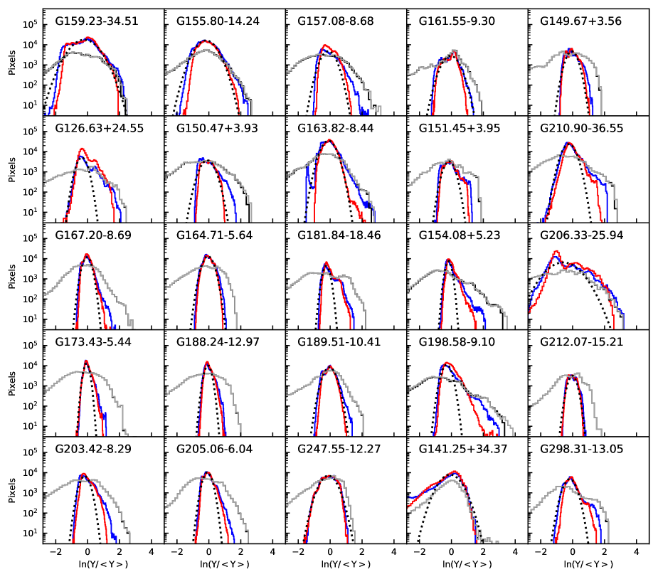
Figure 20: PDFs of the logarithm of the relative values of column density ($N/\langle N\rangle)$; blue lines) and 250$\mu$m surface brightness ($S(250\mu{\rm m})/\langle S(250\mu{\rm m})\rangle)$; red lines). Gaussian fits to the column density histograms are shown as dotted black lines. The black histograms are derived from column density that is estimated based on background subtracted surface-brightness data. The grey histograms additionally (mostly on top of the black histograms) include the bias corrections derived from RT models. The fields are arranged in the order of increasing distance (see Table 1).

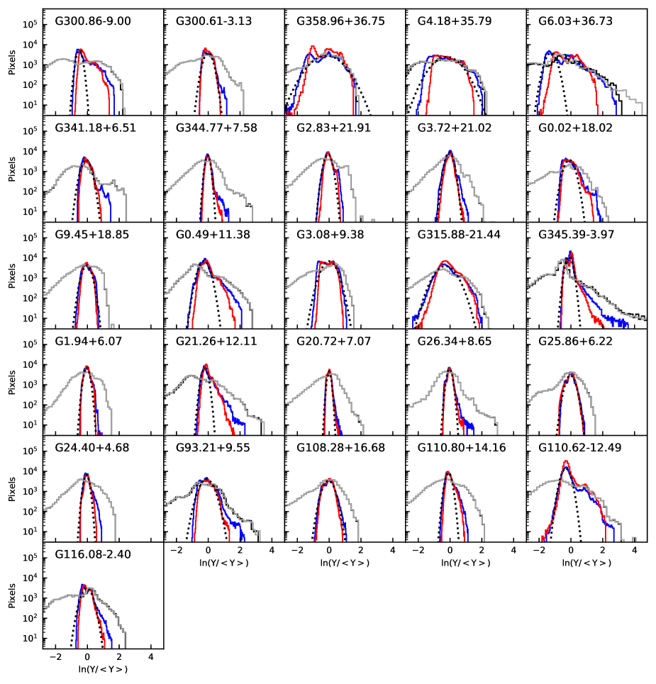
Figure 1: continued.

Appendix B Examples of residuals in radiative transfer models

The radiative transfer modelling is described in Sect. 3.2 with result presented in Sect. 4.4. In most cases the surface-brightness residuals are of the order of 1% and spatially uncorrelated. However, in some fields there are significant, spatially correlated residuals that tend to be related to the properties of the radiation field. The following Figures show three examples where the residuals are caused either by a radiation sources within the field (Fig. 2), a strong anisotropy of the external field (Fig. 3), or by an apparent inconsistency between the heating of the dense and low-density regions (Fig. 4).

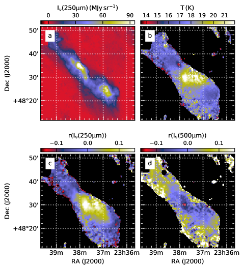
Figure 2: Observed 250 $\mu$m surface brightness $I_{\rm nu}(250\mu{\rm m})$ (frame a), colour temperature $T$ (frame b), and the 250 $\mu$m (frame c) and 500 $\mu$m (frame c) residuals in the RT model of the field G110.62-12.49. Colour temperature is estimated from observations using $\beta=1.8$. The residuals are calculated as $r=(I_{\rm Obs}-I_{\rm Mod})/I_{\rm Obs}$, where Obs and Mod refer to observed and modelled values, respectively. All maps are at 40$\arcsec$ resolution.

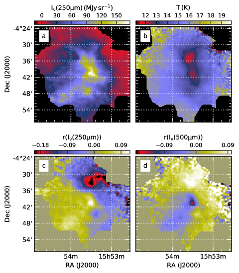
Figure 3: As Fig. 2 but showing the fit residuals for the field G4.18+35.79.

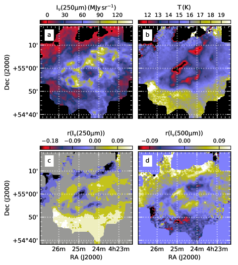
Figure 4: As Fig. 2 but showing fit residuals for the field G150.47+3.93.

Appendix C Clump profile fits with 2D models

The following Figures show the distributions of the 2D fits to a sample of 85 clumps, each with an area close to 10 arcmin².

Figure 5 shows the results for 2D Gaussian fits. Even this simple model gives relatively good fits with rms residuals mostly below 10%. Most pairs of parameters do not show significant correlations. In particular, the angular size and the shape of the clumps are independent of the $\tau(250\mu{\rm m})$ values of both the background and the clump. Similarly, there is no dependence on the estimated distance, apart from the expected correlation with the absolute size of the clumps, for which the correlation coefficient is $r=0.81$. Even if the physical size were completely uncorrelated with the distance, this amount of apparent correlation could be produced by having 30% uncertainty in the distance estimates. Statistically, there is no significant difference between the parameter values obtained with and without the column density corrections derived from the RT models ($N_{\rm cor}$ vs. $N_{\rm obs}$).

In theory, to better characterise the radial profiles of the clumps, one can fit the clumps with Plummer functions (see Eq. (7)). The results of these fits are shown in Fig. 6. However, because of the large number of parameters and the dependence between the $R$ and $p$ parameters, the fitted values show a large scatter. There is a significant positive correlation between the optical depths of the target and the background ($r=0.64$). There is a weaker negative correlation between the clump elongation and the $p$ parameter, which is natural if the source is reminiscent of a cylinder.

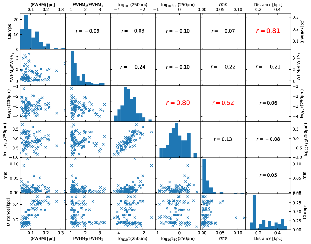
Figure 5: Distributions of the parameters of 2D Gaussian fits to the sub-sample of 85 clumps. The frames in the lower left part of the Figure show scatterplots between the quantities: clump size $\langle{\rm FWHM}\rangle$, clump elongation ${\rm FWHM_{2}/FWHM_{1}}$, peak optical depth $\tau(250\mu{\rm m})$, background optical depth $\tau_{\rm BG}(250\mu{\rm m})$, the relative rms error of the fit, and the distance. The frames on the diagonal show the histograms of the individual quantities and each of the remaining frames indicates the linear correlation coefficient between the corresponding pair of parameters.

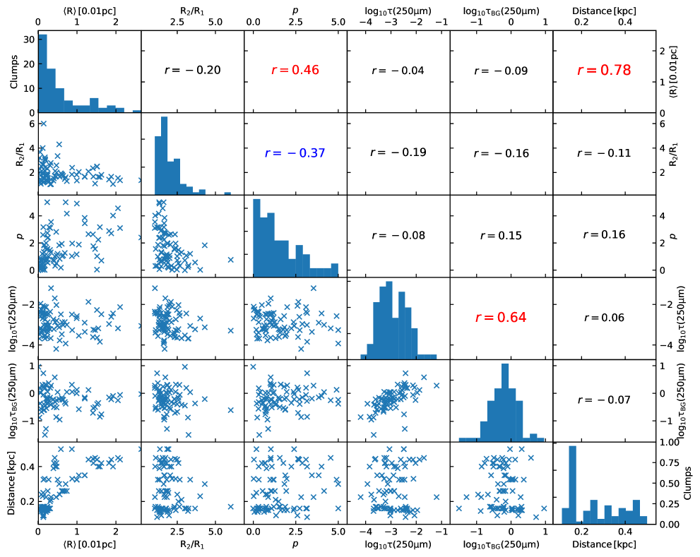
Figure 6: Distributions of the parameters of 2D Plummer profiles for the sub-sample of 85 clumps. Scatterplots and correlations are shown between geometric mean of the flat radius values $\langle R\rangle$, ratio of flat radius values ${\rm R_{2}/R_{1}}$, power-law exponent $p$, peak optical depth $\tau(250\mu{\rm m})$, background optical depth $\tau_{\rm BG}(250\mu{\rm m})$, and distance. The frames on the diagonal show the histograms of the individual quantities and the frames in the upper right hand part of the Figure indicate the linear correlation coefficients for the corresponding pairs of parameters.

Appendix D Examples of cloud structure extracted with TM

Figure 7 shows examples of structures extracted at the 0.6$\arcmin$ and 5$\arcmin$ scales. The fields G181.84-18.46 and G300.86-9.00 are both dominated by a single filamentary structure. However, in Fig. 10, they represent extreme cases where the small- and large-scale structures are either aligned or preferentially perpendicular.

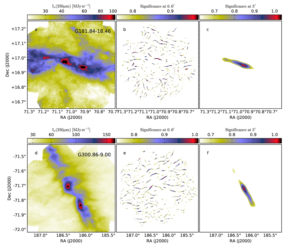
Figure 7: Examples of elongated structures extracted by the TM method. The upper row shows data for the field G181.84-18.46 and the lower row for G300.86-9.00. The frames, from left to right, are the 250 $\mu$m surface brightness and the relative significance of the aligned structures at the 0.6$\arcmin$ and 5$\arcmin$ scales. In the latter frames, pixels with relative significance below the 90% percentile are masked.

Appendix E Angular dispersion functions

The angular dispersion function

$$S(r,\delta)=\sqrt{\frac{1}{N}\sum_{i=1}^{N}\left(\theta(r)-\theta(r+\delta_{i})\right)^{2}},$$ (10)

measures the coherence of angles $\theta$ around a position $r$ as the function of the lag $delta$. The summation goes over all displacements $\delta_{i}$ of a given distance or a distance range. For example, (Planck Collaboration et al. 2015) calculated the coherence of polarisation angles using a wide annulus of [$\delta/2$, $3\delta/2$].

We apply $S$ to the TM results that characterise the structural anisotropy of the surface-brightness images. The possible values of $\delta$ are limited by the typical size of the images and, on the other hand, by the size of the template used in the TM calculation. Depending on the TM parameters (the scale $F$ and the possible normalisation, as described in Sect 3.1) result in the extraction of structures of different size and would thus also change the subsequent estimates of $S$. The position angles $\theta$ that are determined by TM are significant only for a small subset of the map pixels. The sum in Eq. (10) should only include pixels in well-defined structures, but the number of such structures in a given environment can become small, especially for small values of $\delta$.

As an example, we examine $S$ using the TM position angle estimates calculated with the scale parameter $F=1.2\arcmin$ and using data normalisation (see Sect. 3.1) to extract structures more uniformly over the whole map area. Figure 8 compares the map-averaged values of $S$ for two cases where the reference annulus extends over $\theta$=2.4-3.5$\arcmin$ or over larger distances $\theta$=3.6-6.0$\arcmin$. We note that at a distance of 2.4$\arcmin$ the $\theta$ estimates are not completely independent because of the combined effect of the size of the template that was used to estimate the position angles ($2.4\arcmin\times 2.4\arcmin$) and the resolution of the underlying data (18$\arcsec$ for the 250 $\mu$m surface-brightness images).

As expected, the $S$ values at the different scales are correlated and larger lags tend to correspond to larger dispersion (in Fig. 8 on average by 34%). The smallest $S$ values are found for the nearby ($d<200$ pc) fields G300.86-9.00 and G298.31-13.05 that are dominated by one or two filamentary structures close to the scale $F$ selected in TM. Small values are also found for the high-latitude Lynds clouds G358.96+36.75, G6.03+36.73, and G4.18+35.79 (LDN 1780, LDN 183, and LDN 134, respectively). Conversely, the angular dispersion is large in fields like G344.77+7.48 and G345.39-3.97, where most of the area is covered by low-column-density material that has structure more consistent with generic turbulent fluctuations.

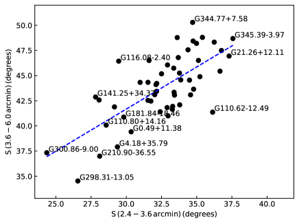
Figure 8: Angular dispersion function $S$ calculated from the position angle estimates of the TM method. The plotted values are averages over individual fields, calculated using lags $\delta$ within the ranges of 2.4-3.5$\arcmin$ and 3.6-6.0$\arcmin$. The dashed line corresponds to the unweighted least squares fit.

Appendix F Radial clump profiles

The Figs. 9-23 show azimuthally averaged column density profiles for clumps with approximate size of 10 arcmin². We have restricted the sample to 85 clumps where the structures do not contain significant secondary peaks.

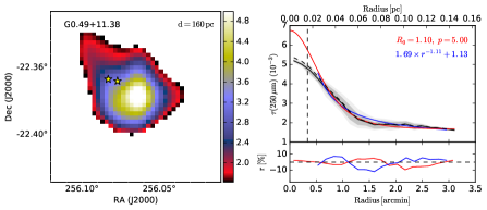
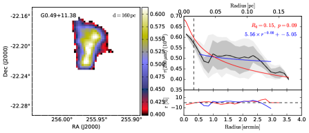
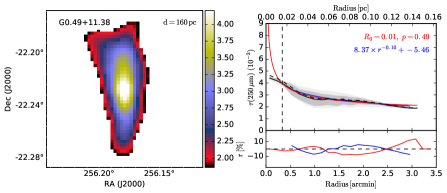
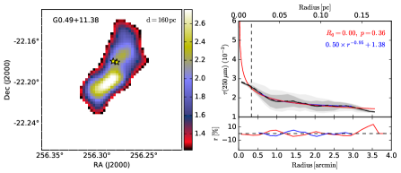
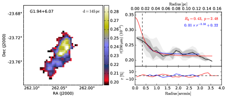
Figure 9: Maps and radial profiles of $10^{-3}\times\tau(250\mu{\rm m})$ for 10 arcmin² clumps. On the map, YSO candidates (Montillaud et al. 2015) are indicated with stars. On the right, the azimuthal averaged profiles are shown without (black solid line) and with (dashed black line) corrections derived from RT models. The shaded areas show the 10-90% and the 25-75% intervals for the azimuthal variation. The red curve correspond to the fitted, de-convolved Plummer profiles. The blue curve correspond to a powerlaw fit to data outside 30$\arcsec$ radius (data corrected according to the RT models but not deconvolved). The fit parameters are quoted in the frame. The vertical dashed line at 20$\arcsec$ corresponds to the FWHM extent of a point source. The lower frame shows the relative fit errors.

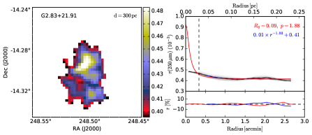
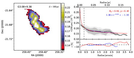
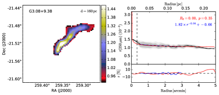
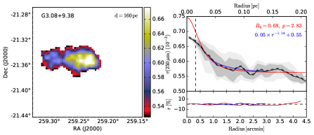
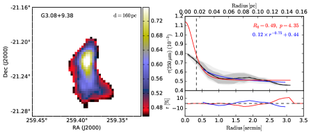
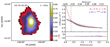
Figure 10: continued.

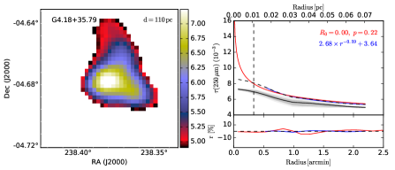
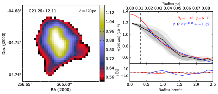
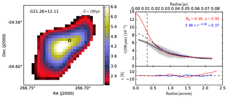
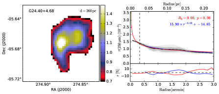
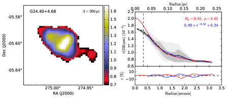
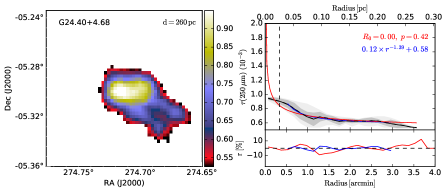
Figure 11: continued.

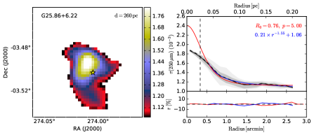
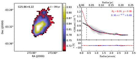
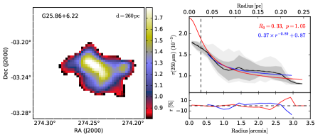
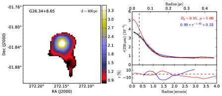
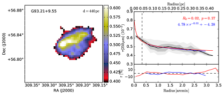
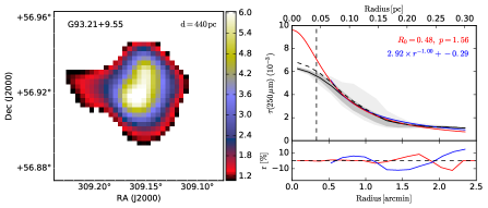
Figure 12: continued.

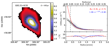
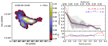
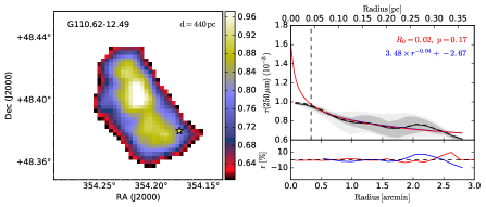
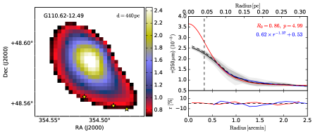
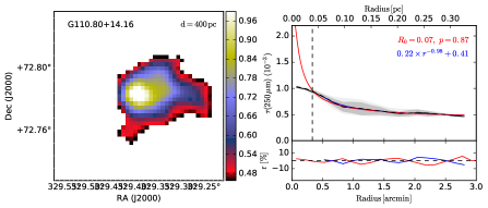
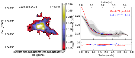
Figure 13: continued.

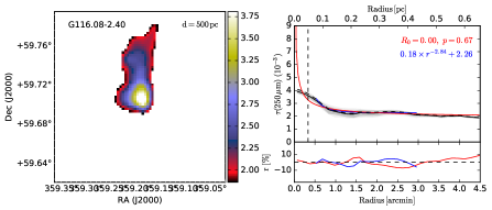
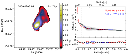
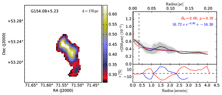
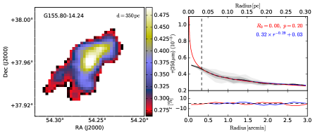
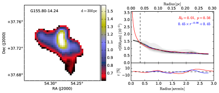
Figure 14: continued.

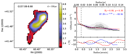
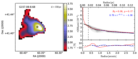
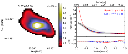
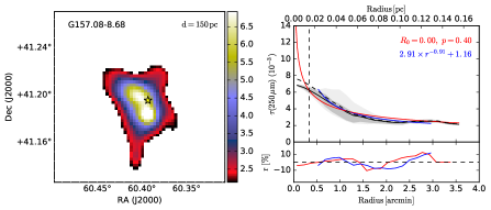
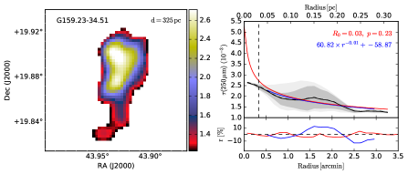
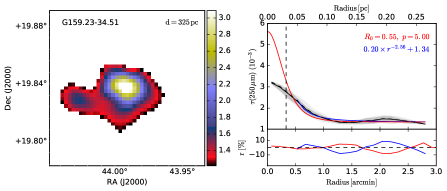
Figure 15: continued.

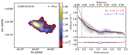
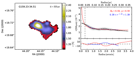
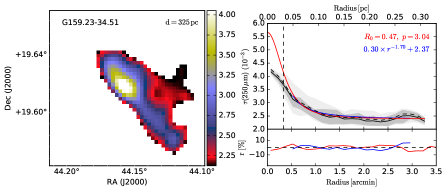
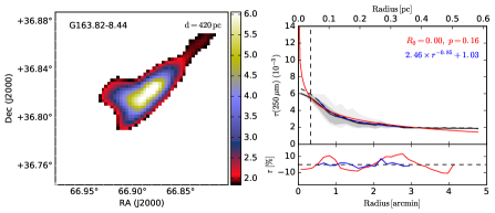
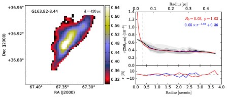
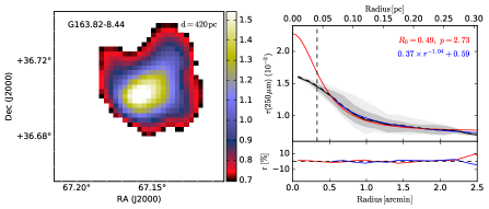
Figure 16: continued.

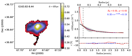
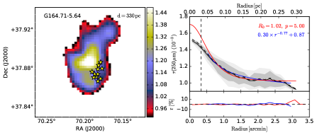
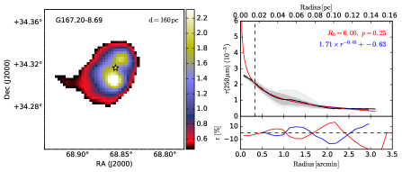
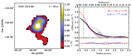
Figure 17: continued.

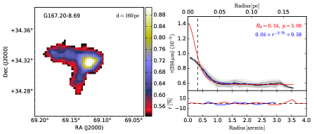
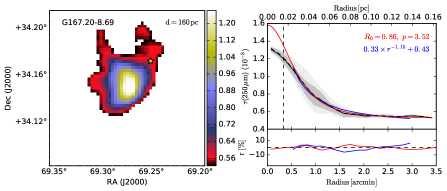
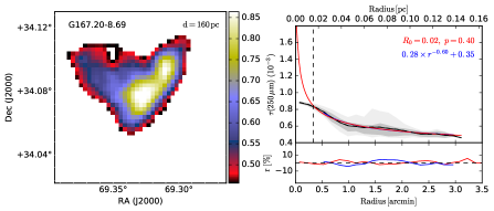
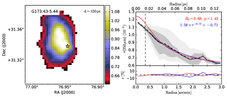
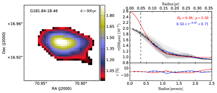
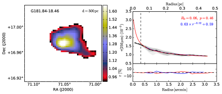
Figure 18: continued.

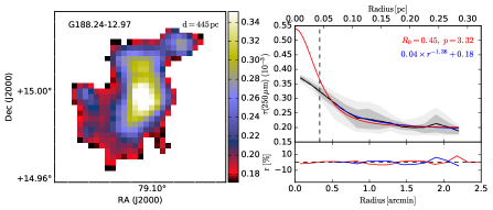
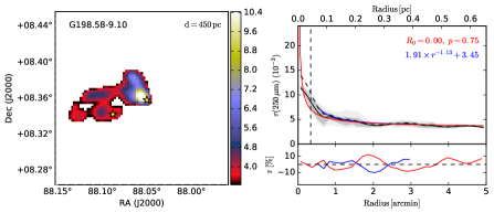
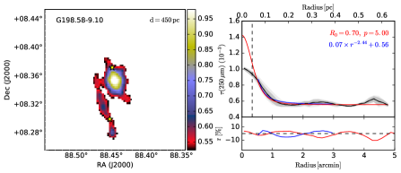
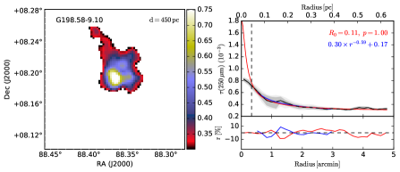
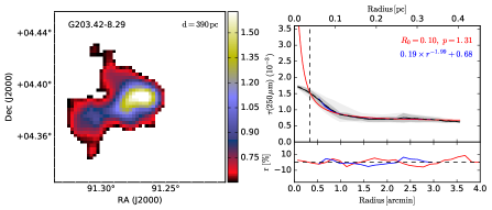
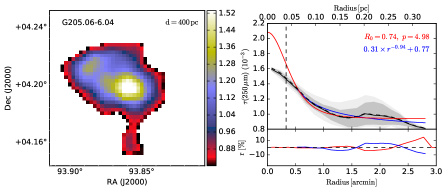
Figure 19: continued.

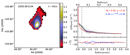
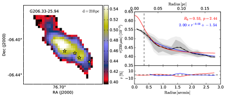
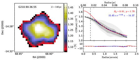
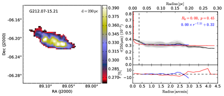
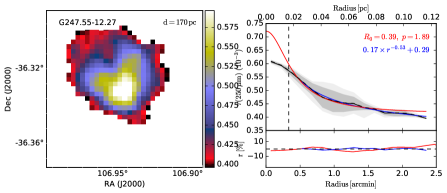
Figure 20: continued.

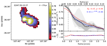
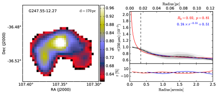
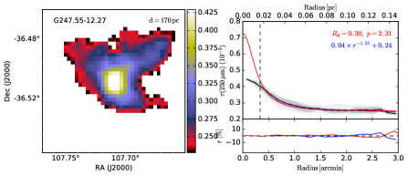
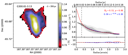
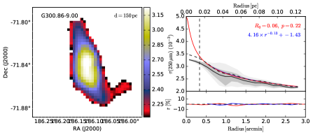
Figure 21: continued.

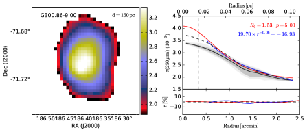
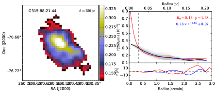
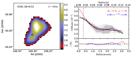
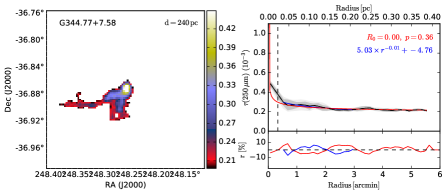
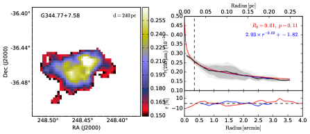
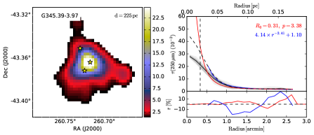
Figure 22: continued.

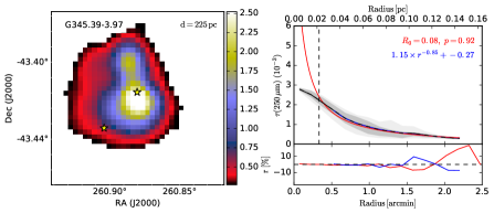
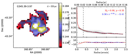
Figure 23: continued.

Appendix G Column density PDFs of individual fields

We noted in Sect. 5.1.3 the PDFs can sometimes reflect the structure of individual objects rather than the general statistical cloud properties. This is true especially because our observations target pre-selected column density peaks.

Before background subtraction, the widest PDF is found in G206.33-25.94, a single cometary cloud observed towards an empty high-latitude sky ($b=-26\degr$). The PDF directly reflects the mass distribution with a dense cloud head and a progressively more diffuse tail. In contrast, fields G20.72+7.07 and G1.94+6.07 have very narrow PDFs. They do not have any particular morphological features and simply happen to consist of structures of nearly uniform column density.

Fields G154.08+5.23, G198.58-9.10, and G345.39-3.97 exhibit well-defined power-law tails towards high column densities. The latter two are clear interface regions with significant column density gradients and a dense boundary layer. Although the boundary layers may contain some cores, the PDF shapes are connected to the particular structure created by external forcing. The third field, G154.08+5.23, looks more like a normal turbulent field. However, also here the PDF tail is associated to elongated high-density regions. This could again be a sharp cloud boundary that is seen more face-on than in the previous examples. PDF shapes are of course also generally affected by projection effects (Schneider et al. 2015b).

There are a couple of fields where the PDF has a long tail towards low column densities. G206.33-25.94 consist of a single cometary cloud and the tail of the PDF directly corresponds to the tail of the cloud. In G141.25+34.37, the PDF asymmetry is even more pronounced but mainly reflects the density profile of the cloud. The average column density of the G141.25+34.37 field is very low and the contribution of the extragalactic background is noticeable. The tail at the low-$N$ side is, of course, very sensitive to the zero point of the quantity used or how the background subtraction is carried out.

Differences between surface brightness and column density PDFs should be correlated with high column density that makes large temperature gradients possible. Anisotropic illumination can have a similar effect. Therefore it may be significant that the difference between surface brightness and column density PDFs is particularly large in the aforementioned fields G198.58-9.10 and G345.39-3.97, both of which exhibit sharp cloud edges.