Factorization and resummation: A new paradigm to improve
gravitational wave amplitudes. II: the higher multipolar modes.

Abstract

The factorization and resummation approach of Nagar and Shah [Phys. Rev. D 94 (2016), 104017], designed to improve the strong-field behavior of the post-Newtonian (PN) residual waveform amplitudes $f_{\ell m}$’s entering the effective-one-body, circularized, gravitational waveform for spinning coalescing binaries, is here improved and generalized to all multipoles up to $\ell=6$. For a test-particle orbiting a Kerr black hole, each multipolar amplitude is truncated at relative 6 post Newtonian (PN) order, both for the orbital (nonspinning) and spin factors. By taking a certain Padé approximant (typically the $P^{4}_{2}$ one) of the orbital factor in conjuction with the inverse Taylor (iResum) representation of the spin factor, it is possible to push the analytical/numerical agreement of the energy fluxe at the level of $5\%$ at the last-stable-orbit for a quasi-maximally spinning black hole with dimensionless spin parameter $+0.99$. When the procedure is generalized to comparable-mass binaries, each orbital factor is kept at relative $3^{+3}$PN order, i.e. the 3PN comparable-mass terms are hybridized with higher PN test-particle terms up to 6PN relative order. The same Padé resummation is used for continuity. By contrast, the spin factor is only kept at the highest comparable-mass PN-order currently available. We illustrate that the consistency between different truncations in the spin content of the waveform amplitudes is stronger in the resummed case than when using the standard Taylor-expanded form of Pan et al. [Phys. Rev. D 83 (2011) 064003]. We finally introduce a method to consistently hybridize comparable-mass and test-particle information also in the presence of spin (including the spin of the particle), discussing it explicitly for the $\ell=m=2$ spin-orbit and spin-square terms. The improved, factorized and resummed, multipolar waveform amplitudes presented here are expected to set a new standard for effective-one-body-based gravitational waveform models.

I Introduction

The parameter estimation of gravitational wave events Abbott et al. (2016a, b, b, 2017a, 2017b, 2017c, 2017d) relies on analytical waveforms models, possibly calibrated (or informed) by Numerical Relativity simulations Taracchini et al. (2014a); Hannam et al. ; Schmidt et al. (2015); Khan et al. (2016); Nagar et al. (2016); Babak et al. (2017); Bohe et al. (2017); Nagar et al. (2017). The effective-one-body (EOB) model is currently the only analytical model available that can be consistently used for analyzing both black hole binaries and neutron star binaries Damour and Nagar (2010); Bernuzzi et al. (2015); Lackey et al. (2017); Hinderer et al. (2016); Steinhoff et al. (2016); Dietrich and Hinderer (2017). One of the central building blocks of the model is the factorized and resummed (circularized) multipolar post-Newtonian (PN) waveform introduced in Damour et al. (2009) for nonspinning binaries. This approach was then straightforwardly generalized in Pan et al. (2011) to spinning binaries. Already Ref. Pan et al. (2011) pointed out that, in the test-particle limit, the amplitude of such resummed waveform gets inaccurate in the strong-field, fast velocity regime, when the spin of the central black hole is $\gtrsim 0.7$. In the same study, an alternative factorization to improve the test-mass waveform behavior also for larger values of the spin was discussed. More pragmatically, Ref. Taracchini et al. (2013) finally suggested to improve the analytical multipolar waveform amplitude (and fluxes) of Pan et al. (2011) by fitting a few parameters, describing effective high-PN orders, to the highly-accurate fluxes obtained solving numerically the Teukolsky equation Hughes et al. (2005). Although this approach is certainly useful to reliably improve the radiation reaction force that drives the transition from quasi-circular inspiral to plunge Taracchini et al. (2014b); Harms et al. (2014); Nagar et al. (2014) for a large mass-ratio binary, the question remains whether the domain of validity of purely analytical results can be enlarged in some way. This question makes special sense nowadays, since PN calculations of the fluxes are available at high order Fujita (2015); Shah (2014) and one would like to use then at best. In addition, following for example the seminal attitude of Refs. Damour and Nagar (2007); Damour et al. (2009), one has to keep in mind that the test-particle limit should always be seen as a useful theoretical laboratory to implement new methods and test new ideas that could be transferred, after suitable modifications, to the case of comparable-mass binaries.

Reference Nagar and Shah (2016) gave a fresh cut to this problem by exploring a new way of treating the residual, PN-expanded, amplitude corrections to the waveforms (i.e., the outcome of the factorization of Refs. Damour et al. (2009); Pan et al. (2011)) that consists of: (i) factorizing it in a purely orbital and a purely spin-dependent part; (ii) separately resumming each factor in various ways, notably using the inverse Taylor (“iResum”) approximant for the spin-dependent factor. Using the test-particle limit to probe the approach, Ref. Nagar and Shah (2016) showed that such factorization–and–resummation paradigm yields a rather good agreement between the $\ell=2$ numerical and analytical waveform amplitudes up to (and often beyond) the last stable orbit (LSO). The contextual preliminary analysis of the comparable-mass case of Nagar and Shah (2016) also suggests that such improved waveform amplitudes are more robust than the standard ones and may eventually need less important NR-calibration via the next-to-quasi-circular correction factor Damour and Nagar (2007).

The purpose of this paper is to deepen and refine the investigation of Ref. Nagar and Shah (2016) as well as to generalize it to higher multipoles up to $\ell=6$. The paper is organized as follows. In Sec. II we review and improve the test-particle results of Nagar and Shah (2016) and generalize the procedure up to $\ell=6$ modes. Section III brings together all the PN-expanded results currently available for the spin-dependent waveform amplitudes Bohe et al. (2013a); Marsat (2015); Bohe et al. (2015), notably written in multipolar form, while Sec. IV explicitly shows the spin-dependent part of the factorized residual amplitudes, both in the standard form of Damour et al. (2009); Pan et al. (2011), and with the factorization of the orbital terms. The approach to the resummation is undertaken in Sec. V, in particular by discussing the hybridization (notably of the orbital terms) with the test-particle information. After the conclusions, Sec. VI the paper is completed by an Appendix that lists all the currently known, PN-expanded, $\nu$-dependent, energy fluxes up to next-to-next-to-leading order in the spin orbit interaction (which include also next-to-leading-order for the spin-spin-terms and leading-order for spin-cube terms). We use units with $c=G=1$.

II Test-particle limit: improving the residual multipolar amplitudes

The purpose of this Section is to review and improve the test-particle results of Ref. Nagar and Shah (2016) for the $\ell=2$ multipole and then generalize them to all multipoles up to $\ell=6$. Let us recall our notation for the multipolar waveform for a circularized, nonprecessing, binary with total mass $M$ and (dimensionful) spins $S_{1}$ and $S_{2}$. To start with, following Ref. Damour et al. (2009) (see e.g. Eq. (75)-(78) there), each waveform multipole is written as

$$h_{\ell m}(x)=h_{\ell m}^{(N,\epsilon)}\hat{h}_{\ell m}^{(\epsilon)},$$ (1)

where $x=(GM\Omega/c^{3})^{2/3}={\cal O}(c^{-2})$ is the PN-ordering frequency parameter ($\Omega$ is the orbital frequency) [we recall that $n$-PN order means ${\cal O}(c^{-2n})$]; $h_{\ell m}^{(N,\epsilon)}$ is the Newtonian (leading-order) contribution to the given $(\ell,m)$ multipole, where $\epsilon=0,1$ is the parity of $\ell+m$ (see Eq. (78) of Damour et al. (2009) and Eq. (88) in Appendix), while $\hat{h}_{\ell m}^{(\epsilon)}$ is the PN correction. Such PN correction is then written in factorized form Damour et al. (2009) as

$$\hat{h}_{\ell m}(x)=\hat{S}_{\rm eff}^{(\epsilon)}\hat{h}_{\ell m}^{\rm tail}f_{\ell m}(x,S_{1},S_{2}).$$ (2)

Here, the first factor, $\hat{S}^{(\epsilon)}_{\rm eff}$ , is the parity-dependent effective source term Damour et al. (2009), define as the EOB effective energy along circular orbits, for $\epsilon=0$, or the Newton-normalized orbital angular momentum, for $\epsilon=1$; the second factor, $\hat{h}_{\ell m}^{\rm tail}\equiv T_{\ell m}e^{\rm i\delta_{\ell m}}$ is a complex factor that accounts for the effect of the tails and other phase-related effects Damour et al. (2009); Mano et al. (1996); Faye et al. (2015); the third factor, $f_{\ell m}$ is the residual amplitude correction. This latter factor can be further resummed in various ways, that notably depend, when $\nu\neq 0$ and $S_{1,2}\neq 0$, on the parity of $m$. For example, the original proposal of Damour et al. (2009), implemented when the objects are nonspinning, was to first compute from the $f_{\ell m}$ the (Taylor-expanded) functions

$$\rho_{\ell m}\equiv T_{n}\left[(f_{\ell m})^{1/\ell}\right],$$ (3)

where $T_{n}[\dots]$ indicates the Taylor expansion up to $x^{n}$ and then define the resummed $f_{\ell m}$ by replacing their Taylor expansions with $(\rho_{{\ell m}})^{\ell}$. When spins are present, the $\rho_{\ell m}$ functions are naturally written as the sum of an orbital (spin-independent) and a spin-dependent contribution as

$$\rho_{\ell m}=\rho_{\ell m}^{\rm orb}+\rho_{\ell m}^{\rm S}.$$ (4)

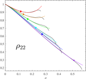
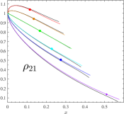
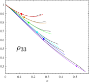
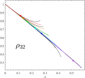
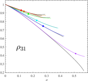
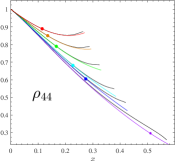
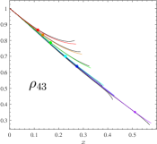
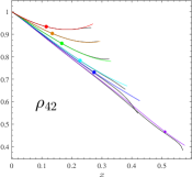
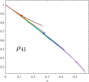
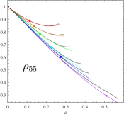
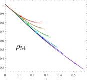
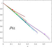
Figure 1: Comparison between the factorized and resummed analytical $\rho_{\ell m}$’s (colored online) and the corresponding numerical (exact) functions (black online) up to $\ell=6$ for values of the BH dimensionless spin ${\hat{a}}{a}=(-0.99,-0.5,0,+0.5,+0.99)$ (red, orange, green, cyan, blue and purple respectively). The filled circles mark the LSO location. This plot is obtained using relative 6PN information for all modes except $\rho_{32}$ that employs 5PN relative accuracy for $\rho_{32}^{\rm orb}$. The Padé approximants used on $\rho_{\ell m}^{\rm orb}$ are listed in second column of Table 1. The same table also lists the numerical/analytical relative difference at the LSO. The agreement remains good (except for few exceptions, see text for details) also for ${\hat{a}}=+0.99$.

Reference Nagar and Shah (2016) proposed then to improve the strong-field behavior of the $\rho_{\ell m}$’s functions by (i) writing them as the product of a purely orbital and purely spin-dependent factors as

$$\rho_{{\ell m}}=\rho_{{\ell m}}^{\rm orb}\hat{\rho}^{\rm S}_{\ell m},$$ (5)

where $\hat{\rho}^{\rm S}_{{\ell m}}\equiv T_{n}[1+\rho_{\ell m}^{\rm S}/\rho^{\rm orb}_{\ell m}]$, and then resumming each separate factor in a certain way that we detail below Although there is no first-principle reason for treating the orbital and spin contributions as separate multiplicative factors, such representation proved useful for interpreting the global behavior of the $\rho_{\ell m}$’s as well as for improving it near (or even below) the LSO. For instance, it was argued that a sort of compensation between the spin and orbital factors should occurr in order to guarantee a good agreement between the numerical and analytical functions close to the LSO, especially for large and positive values of the black hole spin. To accomplish such effect, it is necessary to resum each factor (or at least the spin-dependent one), that is given by a truncated Taylor series, in a specific way. In particular, it was suggested Nagar and Shah (2016) that a simple and efficient method to temperate the divergent behavior of $\hat{\rho}^{\rm S}_{\ell m}$ towards the LSO is to take its inverse Taylor series (or inverse resummed representation, “iResum”) defined as

$$\bar{\rho}_{\ell m}^{\rm S}=\left(T_{n}\left[\left(\hat{\rho}^{\rm S}_{\ell m}(x)\right)^{-1}\right]\right)^{-1}.$$ (6)

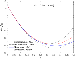
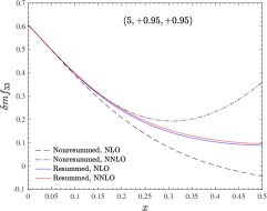
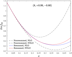
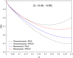
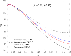
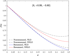
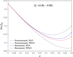
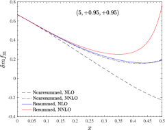
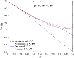
Figure 4: Nonresummed (black) and resummed (colored) residual waveform amplitudes for $\ell=3$ multipoles. The orbital factors are taken at $3^{+3}$ PN relative accuracy except for the $(3,1)$ mode, that is taken at $3^{+2}$ PN level. Likewise the $\ell=2$ case of Fig. 3, the consistency between NLO and NNLO truncations of the spin terms is is improved by the resummation.

Reference Nagar and Shah (2016) illustrated that, due to the large amount of PN information available, it is possible to achieve satisfactory numerical/analytical agreement using different truncated PN series as a starting point, though lower-PN orders (e.g. 6PN) are preferable with respect to high-PN orders (e.g. 10PN or 20PN). The analysis Nagar and Shah (2016) also showed that, once that the factorization and resummation paradigm is assumed, one is free to choose at what PN order to work, provided the resummed amplitude shows a good agreement with the numerical curves. For consistency with previous, EOB-related, works Damour and Nagar (2014), in Nagar and Shah (2016) it was chosen to keep the orbital part at 5PN order, and in Taylor-expanded form, together with the spin-dependent factor truncated at 3.5PN. This choice was made so to be consistent with the spin-dependent information used in the comparable-mass case. For the $\ell=m=2$ multipole, this yielded rather acceptable analytical/numerical agreement ($\simeq 1\%$) up to the LSO for all spin values between $-0.99$ and $+0.99$ (see Fig. 4 of Nagar and Shah (2016)).

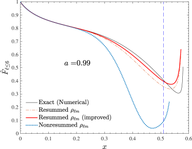
Figure 2: Test-particle limit: comparison between analytical and exact (numerical) fluxes for dimensionless black-hole spin $\hat{a}=+0.99$. The functions $\rho_{33}^{\rm orb}$, $\rho_{44}^{\rm orb}$ and $\rho_{55}^{\rm orb}$ are either resummed using (4,2) Padé approximants (orange, dot-dashed line) or kept in PN-expanded form up to (relative) 6PN order. This second choice improves the agreement with the numerical curve. The dotted line represents the analytical flux where the total 6PN-accurate $\rho_{\ell m}$’s are kept in the standard, nonfactorized, Taylor-expanded form.

Table 1: Fractional differences between the resummed and the numerical $\rho_{\ell}$’s at the LSO. From left to right the columns report: the multipolar order; the Padé approximant chosen for the orbital factor; the PN order chosen for the spin-dependent factors; the fractional difference $(\rho^{\rm num}-\rho^{\rm anlyt})/\rho^{\rm num}$ at $x_{\rm LSO}$.

$(\ell,m)$	$P^{i}_{j}(\rho^{orb}_{\ell m})$	$iR$(PN)	$\Delta(x)\rho(x)/\rho|_{x=x_{\rm LSO}}$ for $-0.99\leq\hat{a}\leq+0.99$
			$-0.99$	$-0.5$	$0$	$+0.5$	$+0.7$	$+0.99$
$(2,2)$	$P^{4}_{2}$	$6$	$-1\times 10^{-4}$	$-3\times 10^{-4}$	$-6\times 10^{-4}$	$-0.002$	$-0.004$	$0.026$
$(2,1)$	$P^{5}_{1}$	$6$	$-0.006$	$-0.004$	$2\times 10^{-5}$	$0.010$	$0.019$	$0.159$
$(3,3)$	$P^{4}_{2}$	$6$	$-4\times 10^{-5}$	$-1\times 10^{-4}$	$-4\times 10^{-4}$	$-0.002$	$-0.005$	$-0.058$
(3,3)	$P^{6}_{0}$	$6$	$-2\times 10^{-5}$	$-6\times 10^{-5}$	$-2\times 10^{-4}$	$-0.001$	$-0.002$	$-0.023$
$(3,2)$	$P^{4}_{2}$	$6$	$-0.004$	$-0.003$	$-5\times 10^{-5}$	$0.006$	$0.012$	$-0.026$
$(3,1)$	$P^{3}_{2}$	$6$	$-3\times 10^{-5}$	$-6\times 10^{-5}$	$-1\times 10^{-4}$	$-3\times 10^{-4}$	$-8\times 10^{-5}$	$0.248$
(3,1)	$P^{3}_{1}$	$8$	$-2\times 10^{-5}$	$-4\times 10^{-5}$	$-1\times 10^{-4}$	$-8\times 10^{-4}$	$-0.002$	$-0.0017$
$(4,4)$	$P^{4}_{2}$	$6$	$-2\times 10^{-5}$	$-8\times 10^{-5}$	$-3\times 10^{-4}$	$-0.002$	$-0.005$	$-0.088$
(4,4)	$P^{6}_{0}$	$6$	$-4\times 10^{-6}$	$-3\times 10^{-5}$	$-2\times 10^{-4}$	$-0.001$	$-0.002$	$-0.046$
$(4,3)$	$P^{4}_{2}$	$6$	$-0.003$	$-0.002$	$-1\times 10^{-4}$	$0.004$	$0.008$	$0.004$
$(4,2)$	$P^{6}_{0}$	$6$	$-1\times 10^{-5}$	$-2\times 10^{-5}$	$-5\times 10^{-5}$	$6\times 10^{-4}$	$0.003$	$0.015$
$(4,1)$	$P^{4}_{2}$	$6$	$-0.003$	$-0.002$	$8\times 10^{-6}$	$0.005$	$0.008$	$-0.013$
(5,5)	$P^{4}_{2}$	$6$	$-2\times 10^{-5}$	$-7\times 10^{-5}$	$-3\times 10^{-4}$	$-0.002$	$-0.037$	$-0.101$
(5,5)	$P^{6}_{0}$	$6$	$2\times 10^{-6}$	$-2\times 10^{-5}$	$-1\times 10^{-4}$	$-0.001$	$-0.034$	$-0.054$
$(5,4)$	$P^{4}_{2}$	$6$	$-0.003$	$-0.002$	$-2\times 10^{-4}$	$0.003$	$0.005$	$-0.013$
$(5,3)$	$P^{4}_{2}$	$6$	$-2\times 10^{-5}$	$-6\times 10^{-5}$	$-2\times 10^{-4}$	$-6\times 10^{-4}$	$-7\times 10^{-4}$	$-0.043$
$(5,2)$	$P^{4}_{2}$	$6$	$-0.002$	$-0.002$	$8\times 10^{-6}$	$0.004$	$0.009$	$0.077$
$(5,1)$	$P^{6}_{0}$	$6$	$1\times 10^{-5}$	$1\times 10^{-5}$	$3\times 10^{-5}$	$1\times 10^{-4}$	$5\times 10^{-4}$	$0.101$
$(6,6)$	$P^{4}_{2}$	$5$	$-4\times 10^{-5}$	$-1\times 10^{-4}$	$-3\times 10^{-4}$	$-5\times 10^{-5}$	$0.002$	$0.064$
$(6,5)$	$P^{4}_{2}$	$6$	$-0.002$	$-0.001$	$-2\times 10^{-4}$	$0.002$	$0.003$	$-0.029$
$(6,4)$	$P^{4}_{2}$	$6$	$-2\times 10^{-5}$	$-6\times 10^{-5}$	$-2\times 10^{-4}$	$-8\times 10^{-4}$	$-0.001$	$-0.035$
$(6,3)$	$P^{4}_{2}$	$6$	$-0.002$	$-0.001$	$-1\times 10^{-5}$	$0.003$	$0.007$	$0.053$
$(6,2)$	$P^{4}_{2}$	$6$	$-4\times 10^{-6}$	$-2\times 10^{-5}$	$-5\times 10^{-5}$	$2\times 10^{-5}$	$0.001$	$0.213$
(6,2)	$P^{6}_{2}$	$8$	$-6\times 10^{-7}$	$-8\times 10^{-7}$	$-7\times 10^{-7}$	$8\times 10^{-5}$	$9\times 10^{-4}$	$0.015$
$(6,1)$	$P^{6}_{0}$	$6$	$-0.002$	$-0.001$	$7\times 10^{-6}$	$0.003$	$0.003$	$0.028$

Here we relax the constraint of being consistent with previous EOB-related works and present, instead, a new recipe to further improve $\ell=m=2$ results of Ref. Nagar and Shah (2016) and extend them to higher multipolar modes. To do so, we: (i) generally increase the PN order, possibly requiring it to be the same for both the spin and orbital factors; (ii) resum the orbital factor using some Padé approximant, to be chosen according to the PN order and the multipole; (iii) resum the spin factor taking its inverse Taylor approximant (iResum) as proposed in Nagar and Shah (2016), see Eq. (6) above. We find that, modulo a few exceptions to be detailed below, a good compromise is reached by working at relative 6PN order for each mode and taking a Pade $(4,2)$ approximant for the orbital factor. There are exceptions to this choice (see 2nd column of Table 1). For example, the (2,1) mode is better represented using a $P^{5}_{1}$ approximant, the (3,1) using a $P^{3}_{2}$ (i.e. keeping $\rho_{32}^{\rm orb}$ at 5PN accuracy), while for $(4,2)$, $(5,1)$ and $(6,1)$ the orbital factor in Taylor-expanded form is preferable. These choices are made so that the analytical $\rho_{{\ell m}}$’s remain as close as possible to the numerical one up to the LSO (and possibly beyond). This is illustrated in Fig. 1, which displays all $\rho_{\ell m}$’s functions up $\ell=6$. The figure collects five values of the dimensionless black-hole spin, ${\hat{a}}=(-0.99,-0.5,0,+0.5,+0.99)$. The analytical functions are depicted as colored curves, while the numerical data are black. Both curves extend up to the light-ring, while the filled circle mark the LSO location. The ${\hat{a}}=+0.99$ curves extend up to the highest-frequency (purple, lowest curve) while the ${\hat{a}}=-0.99$ is at the top of each panel and is depicted red. The information encoded in the figure is complemented by Table 1, that lists, for each multipole, the Padé approximant adopted together with the numerical/analytical fractional difference computed at the LSO. The figure also highlights that the numerical/analytical agreement looks improvable (for large values of ${\hat{a}}$) for some subdominant modes, especially $\rho_{31}$ and $\rho_{62}$, where the analytical functions are systematically above the numerical ones towards the boundary of the $x$-domain considered. The reason behind this behavior is that both $P^{3}_{2}(\rho^{\rm orb}_{32})$ and $P^{4}_{2}(\rho^{\rm orb}_{62})$ develop a spurious pole on the real $x$-axis, at $x\approx 0.86$ for the former and at $x\approx 0.82$ for the latter. In this respect, we stress that our choices about the PN truncation order and the consequent resummation strategies should be seen as a compromise between simplicity (i.e. using relatively low-order PN-information) and achievable accuracy (i.e. good global agreement with the numerical functions). For example, one finds that the numerical/analytical disagreement for $\rho_{31}$ at the LSO for $\hat{a}=+0.99$ can be reduced to just $-0.17\%$ by: (i) taking $\rho_{31}^{\rm orb}$ at only 4PN order and resumming it with a $P^{3}_{1}$ approximant, while (ii) $\hat{\rho}^{\rm S}_{31}$ is taken up to 8PN order and then resummed as usual with its inverse Taylor series. Similarly, one also easily finds that the global behavior of the $(3,3)$, $(4,4)$ and $(5,5)$ modes can be improved by just keeping the orbital factor in Taylor-expanded form instead of replacing it with its $(4,2)$ Padé approximant. To figure out the relevance of any of these improvements, it is convenient to inspect the total energy flux reconstructed using the resummed $\rho_{\ell m}$’s. At a practical level, some analytical/numerical differences that look large on the $\rho_{\ell m}$’s are subdominant within the flux and can be practically ignored. Figure 2 compares Newton-normalized energy fluxes, with all multipoles summed together up to $\ell=6$ included, as follows: (i) the exact (numerical) flux; (ii) the analytical flux that is obtained from the $\rho_{\ell m}$’s shown in Fig. 1, where the choices for the Padé of the orbital part are listed as non-bold face in Table 1 (dot-dashed, orange line); (iii) the analytical flux obtained by taking the $\rho_{33}^{\rm orb}$, $\rho_{44}^{\rm orb}$ and $\rho_{55}^{\rm orb}$ as plain 6PN-accurate Taylor expansions; (iv) the analytical flux where the 6PN-accurate $\rho_{\ell m}$ are neither further factorized nor resummed, following the original paradigm of Refs. Damour et al. (2009); Pan et al. (2011). The vertical line marks the LSO location. The figure illustrates how changing the treatment of the orbital part of the subdominant modes mentioned above allows one to reduce the fractional difference around the LSO from $10\%$ to approximately $5\%$. It is also to be noticed the good qualitative behavior of the flux also below the LSO, close to the light ring where the flux diverges. By contrast, the flux obtained using the standard, nonresummed, $\rho_{\ell m}$ amplitudes in the form of Damour et al. (2009); Pan et al. (2011), though pushed to higher PN order as discussed above, is reliable only up to $x\approx 0.2$. We also mention that, even though the choice of $P^{3}_{1}(\rho^{\rm orb}_{31})\bar{\rho}_{31}^{\rm S}$ with $\hat{\rho}^{\rm S}_{31}$ at 8PN order can strongly reduce the numerical/analytical differences displayed in Fig. 1, in practice this does not have any notable consequence on the total flux. The same statement also holds for the $(6,2)$ mode: the near-LSO behavior of the analytical $\rho_{62}$ can be improved by working at 8PN, both in the spin and orbital factors (with a $P^{6}_{2}$ approximant for this latter), without however producing any important impact on the total flux computation.

Let us finally mention in passing that another way to improve the strong-field behavior of the $\rho_{\ell m}$’s (and thus of the flux) is by including some effective high-PN order parameter that can be informed (i.e., calibrated or even fitted) to the numerical data. This approach might be necessary, for example, when dealing with precision calculations that require an accurate representation of the radiation reaction in the near-LSO regime, e.g., estimate of the final recoil velocity when the central black hole is quasi-extremal with the spin aligned with the orbital angular momentum Nagar et al. (2014). As an exploratory investigation dealing with just $\rho_{22}$, we found that it is sufficient to introduce a 6.5PN (effective) parameter at the denominator of $\bar{\rho}^{\rm S}_{22}$ and tune it to reduce by more than an order of magnitude the fractional difference between the analytical and numerical functions up to the LSO. More precisely, we have that $\bar{\rho}^{\rm S}_{22}$ has the structural form $1/(1+\hat{a}x^{3/2}+......+\hat{a}c_{13/2}x^{13/2})$, where $\hat{a}c_{13/2}x^{13/2}$ is formally the first spin-orbit term beyond what we are using in this work. One easily checks that the value $c_{13/2}=5.1$ is sufficient to obtain a fractional disagreement of the order $0.15\%$ at the LSO for $\hat{a}=+0.99$. This illustrative example suggests that there is a simple, though effective, way to incorporate the information encoded in the numerical data within the analytical description of the waveform amplitudes. More work will be needed to put this approach in a more systematic form. In particular one may hope that a suitable modification of this method, probably with a few more parameters, could be used to obtain an accurate, semi-analytic, representation of the circularized fluxes also up to the light-ring.

III Comparable masses: Post-Newtonian expanded results

III.1 Waveform amplitudes: spin-orbit and quadratic-in-spin terms

We start by summarizing here new results for the PN-expanded, nonprecessing, multipolar waveform amplitudes up to: (i) next-to-next-to-leading-order (NNLO) for the spin-orbit terms; (ii) next-to-leading-order (NLO) for the spin-spin terms and (iii) for the leading-order (LO) spin-cube terms. These waveform amplitudes were computed by A. Bohé and S. Marsat Bohe and Marsat (2017) as part of a project that aims at obtaining the complete waveform at this PN order (we recall that the corresponding calculation of the PN-expanded energy flux is complete Bohe et al. (2013b); Marsat et al. (2014); Marsat (2015); Bohe et al. (2015)), and kindly shared with us before publication. Here we only list the PN-expanded multipolar waveform amplitudes with their complete, currently known, spin dependence. For completeness, we also include the known, $\nu$-dependent, orbital terms Kidder (2008). To start with, let us set the notations and define our choice of spin variables. We denote with $\nu=m_{1}m_{2}/M^{2}$ the symmetric mass ratio, with $M=m_{1}+m_{2}$ and we adopt the convention that $m_{1}\geq m_{2}$. From the conserved norm, dimensionful, spin vectors $({\bf S}_{1},{\bf S}_{2})$, PN results are usually expressed in terms of the spin combinations ${\bf S}\equiv{\bf S}_{1}+{\bf S}_{2}$ and ${\bf\Sigma}\equiv M\left({\bf S}_{2}/m_{2}-{\bf S}_{1}/m_{1}\right)$. For spin-aligned binaries, where $\bm{\ell}$ indicates the unit vector normal to the orbital plane (i.e., the direction of the orbital angular momentum), one deals with the projections of the spin-vectors along $\bm{\ell}$, i.e., $S_{\ell}={\bf S}\cdot\bm{\ell}$ and $\Sigma_{\ell}={\bf\Sigma}\cdot\bm{\ell}$. Then, it is common practice to work with dimensionless spin variables $\chi_{1,2}\equiv S_{1,2}/(m_{1,2})^{2}$ and in the PN-expansions the spin vectors always appear divided by the square of the total mass, so that one has

$$\hat{S}_{\ell}\equiv\dfrac{S_{\ell}}{M^{2}} =X_{1}^{2}\chi_{1}+X_{2}^{2}\chi_{2},$$ (7)

$$\hat{\Sigma}_{\ell}\equiv\dfrac{\Sigma_{\ell}}{M^{2}} =X_{2}\chi_{2}-X_{1}\chi_{1},$$ (8)

where we introduced the usual convenient notation $X_{i}\equiv m_{i}/M$, which yields $X_{1}+X_{2}=1$, $X_{1}X_{2}=\nu$ and, since $X_{1}\geq X_{2}$, we have $X_{1}=\left(1+\sqrt{1-4\nu}\right)/2$. From the dimensionless spin variables, the waveform spin-dependence is sometimes also written via their symmetric and antisymmetric combinations (see e.g. Pan et al. (2011); Taracchini et al. (2012); Damour and Nagar (2014); Bohe et al. (2017)), $\chi_{S}\equiv\left(\chi_{1}+\chi_{2}\right)/2$ and $\chi_{A}\equiv\left(\chi_{1}-\chi_{2}\right)/2$.

Here, we express the waveform spin dependence using the Kerr parameters of the two black holes divided by the total mass of the system, namely via the variables

$$\tilde{a}_{i}\equiv\dfrac{a_{i}}{M}=\dfrac{S_{i}}{Mm_{i}}=X_{i}\chi_{i}\qquad i=1,2.$$ (9)

This choice is convenient for two reasons: (i) the analytical expression get more compact as several factors $\sqrt{1-4\nu}$ are absorbed in the definitions, and one can more clearly distinguish the sequence of terms that are “even”, in the sense that are symmetric under exchange of body 1 with body 2 and are proportional to the “total Kerr dimensionless spin” $\hat{a}_{0}\equiv\tilde{a}_{1}+\tilde{a}_{2}$ from those that are “odd”, i.e. change sign under the exchange of body 1 with body 2 and are proportional to the factor $\sqrt{1-4\nu}(\tilde{a}_{1}-\tilde{a}_{2})$; (ii) in addition, one can infer the (spinning) test-particle limit from the general $\nu$-dependent, expressions just by inspecting them visually. In fact, in this limit, $m_{2}\ll m_{1}$, $\tilde{a}_{12}\rightarrow 0$ and $\tilde{a}_{1}$ becomes the dimensionaless spin of the massive black hole of mass $m_{1}\approx M$, $\tilde{a}_{1}\rightarrow S_{1}/(m_{1})^{2}$. Similarly, the spinning particle limit around Kerr is simply obtained by putting $\nu=0$, since $\tilde{a}_{2}$ just reduces to the usual spin-variable used in PN or numerical calculations Tanaka et al. (1996); Harms et al. (2016a, b); Lukes-Gerakopoulos et al. (2017), $\sigma\equiv S_{2}/({m_{1}m_{2}})$. To keep the expressions compact, we also define the following combinations of the $\tilde{a}_{i}$ of Eq. (9)

$${\hat{a}}_{0} \equiv X_{1}\chi_{1}+X_{2}\chi_{2}={\tilde{a}}_{1}+{\tilde{a}}_{2},$$ (10)

$${\tilde{a}}_{12} \equiv{\tilde{a}}_{1}-{\tilde{a}}_{2},$$ (11)

$$X_{12} \equiv X_{1}-X_{2}=\sqrt{1-4\nu}.$$ (12)

Equations (7)-(8) above then simply read

$$\hat{S}_{\ell} =\dfrac{1}{2}\left(\hat{a}_{0}+\tilde{a}_{12}X_{12}\right),$$ (13)

$$\hat{\Sigma}_{\ell} =-\tilde{a}_{12}.$$ (14)

We report below the complete modulus of $\hat{h}_{\ell m}$ up to NNLO in the spin-orbit coupling and up to NLO in the spin-spin coupling. Note however that for the $m={\rm odd}$ multipoles we defactorized the factor $X_{12}$ (that is usually seen as part of the Newtonian prefactor $h_{\ell m}^{(N,\epsilon)}$, see Eq. (1)) to avoid the appearence of a fictitious singularity when $\nu=1/4$ in the spin-dependent terms proportional to $\tilde{a}_{12}$ (see also Taracchini et al. (2012)). To have a consistent notation, when $m={\rm odd}$ we focus on the quantities

$$\tilde{h}_{\ell m}^{(\epsilon)}=X_{12}\hat{h}_{\ell m}^{(\epsilon)}.$$ (15)

In conclusion, the modulus of the Newton-normalized PN-expanded, multipolar, waveform we use as starting point reads:

$$|\hat{h}_{22}^{(0)}| =1+\left(-\frac{107}{42}+\frac{55}{42}\nu\right)x-\biggl{[}-2\pi+\hat{a}_{0}+\frac{1}{3}\tilde{a}_{12}X_{12}\biggr{]}x^{3/2}+\biggl{[}\hat{a}_{0}^{2}-\frac{2173}{1512}-\frac{1069}{216}\nu+\frac{2047}{1512}\nu^{2}\biggr{]}x^{2}$$

$$+\biggl{[}-\pi\left(\dfrac{107}{21}-\dfrac{34}{21}\nu\right)-\hat{a}_{0}\left(\frac{163}{126}+\frac{46}{63}\nu\right)-\tilde{a}_{12}X_{12}\left(\frac{157}{126}+\frac{22}{21}\nu\right)\biggr{]}x^{5/2}$$

$$+\Biggl{\{}\frac{27027409}{646800}-\frac{113}{63}\left(\tilde{a}_{1}^{2}+\frac{271}{113}\tilde{a}_{1}\tilde{a}_{2}+\tilde{a}_{2}^{2}\right)-2\pi\left(\hat{a}_{0}+\frac{1}{3}\tilde{a}_{12}X_{12}\right)+\frac{2}{3}\pi^{2}+\frac{121}{63}\hat{a}_{0}\tilde{a}_{12}X_{12}-\frac{856}{105}{\rm eulerlog}_{2}(x)$$

$$+\biggl{[}-\frac{278185}{33264}+\frac{20}{21}\left(\tilde{a}_{1}^{2}+\frac{24}{5}\tilde{a}_{1}\tilde{a}_{2}+\tilde{a}_{2}^{2}\right)+\frac{41}{96}\pi^{2}\biggr{]}\nu-\frac{20261}{2772}\nu^{2}+\frac{114635}{99792}\nu^{3}\Biggr{\}}x^{3}$$

$$+\biggl{[}\hat{a}_{0}\left(\frac{1061}{168}+\frac{4043}{168}\nu+\frac{499}{168}\nu^{2}\right)+\tilde{a}_{12}X_{12}\left(\frac{241}{216}+\frac{5135}{1512}\nu-\frac{79}{72}\nu^{2}\right)\biggr{]}x^{7/2},$$ (16)

$$|\tilde{h}_{21}^{(1)}| =X_{12}-\frac{3}{2}\tilde{a}_{12}x^{1/2}+X_{12}\left(-\frac{17}{28}+\frac{5}{7}\nu\right)x+\biggl{[}\tilde{a}_{12}\left(\frac{18}{7}+\frac{33}{14}\nu\right)+X_{12}\left(-\frac{43}{14}\hat{a}_{0}+\pi\right)\biggr{]}x^{3/2}$$

$$+\biggl{[}\tilde{a}_{12}\left(\hat{a}_{0}-\frac{3}{2}\pi\right)+X_{12}\biggl{(}-\frac{43}{126}+2\hat{a}_{0}^{2}-2\tilde{a}_{1}\tilde{a}_{2}-\frac{509}{126}\nu+\frac{79}{168}\nu^{2}\biggr{)}\biggr{]}x^{2}$$

$$+\biggl{[}\tilde{a}_{12}\left(-\frac{131}{72}+\frac{5483}{504}\nu+\frac{179}{126}\nu^{2}\right)+\hat{a}_{0}X_{12}\left(-\frac{331}{504}+\frac{193}{63}\nu\right)\biggr{]}x^{5/2},$$ (17)

$$|\tilde{h}_{33}^{(0)}| =X_{12}+X_{12}(-4+2\nu)x+\biggl{[}\tilde{a}_{12}\left(-\frac{1}{4}+\frac{5}{2}\nu\right)+X_{12}\left(-\frac{7}{4}\hat{a}_{0}+3\pi\right)\biggr{]}x^{3/2}$$

$$+X_{12}\biggl{(}\frac{3}{2}\hat{a}_{0}^{2}+\frac{123}{110}-\frac{1838}{165}\nu+\frac{887}{330}\nu^{2}\biggr{)}x^{2}$$

$$+\biggl{[}\tilde{a}_{12}\left(-\frac{119}{60}+\frac{27}{20}\nu+\frac{241}{30}\nu^{2}\right)+\hat{a}_{0}X_{12}\left(\frac{139}{60}-\frac{83}{60}\nu\right)\biggr{]}x^{5/2},$$ (18)

$$|\hat{h}_{32}^{(1)}| =1+\frac{1}{1-3\nu}\biggl{\{}\left(\hat{a}_{0}-\tilde{a}_{12}X_{12}\right)x^{1/2}+\left(-\frac{193}{90}+\frac{145}{18}\nu-\frac{73}{18}\nu^{2}\right)x$$

$$+\frac{1}{6}\biggl{[}\hat{a}_{0}(-39+73\nu)+\tilde{a}_{12}X_{12}(23+13\nu)+12\pi(1-3\nu)\biggr{]}x^{3/2}\biggr{\}},$$ (19)

$$|\tilde{h}_{31}^{(0)}| =X_{12}-\frac{2}{3}X_{12}(4+\nu)x+\biggl{[}\tilde{a}_{12}\left(-\frac{9}{4}+\frac{13}{2}\nu\right)+X_{12}\left(\frac{1}{4}\hat{a}_{0}+\pi\right)\biggr{]}x^{3/2}$$

$$+\biggl{[}-4(\tilde{a}_{1}^{2}+\tilde{a}_{2}^{2})+X_{12}\left(\frac{607}{198}-\frac{136}{99}\nu-\frac{247}{198}\nu^{2}+\frac{3}{2}\hat{a}_{0}^{2}\right)\biggr{]}x^{2}$$

$$+\biggl{[}\tilde{a}_{12}\left(\frac{73}{12}-\frac{641}{36}\nu-\frac{5}{2}\nu^{2}\right)+X_{12}\hat{a}_{0}\left(-\frac{79}{36}+\frac{443}{36}\nu\right)\biggr{]}x^{5/2},$$ (20)

$$|\hat{h}_{44}^{(0)}| =1+\frac{1}{1-3\nu}\biggl{\{}\frac{1}{330}(-1779+6365\nu-2625\nu^{2})x$$

$$+\frac{1}{15}\biggl{[}\hat{a}_{0}(-38+114\nu)+60\pi(1-3\nu)-2\tilde{a}_{12}X_{12}(1-21\nu)\biggr{]}x^{3/2}$$

$$+\biggl{(}\frac{1068671}{200200}-\frac{1088119}{28600}\nu+\frac{146879}{2340}\nu^{2}-\frac{226097}{17160}\nu^{3}\biggr{)}x^{2}\biggr{\}},$$ (21)

$$|\tilde{h}_{43}^{(1)}| =X_{12}+\frac{1}{-1+2\nu}\biggl{\{}\frac{5}{4}\biggl{[}\tilde{a}_{12}(1-2\nu)-\hat{a}_{0}X_{12}\biggr{]}x^{1/2}+X_{12}\left(\frac{39}{11}-\frac{1267}{132}\nu+\frac{131}{33}\nu^{2}\right)x\biggr{\}},$$ (22)

$$|\hat{h}_{42}^{(0)}| =1+\frac{1}{1-3\nu}\biggl{\{}\frac{1}{330}(-1311+4025\nu-285\nu^{2})x$$

$$-\frac{1}{15}\biggl{[}2\hat{a}_{0}(1-3\nu)+\tilde{a}_{12}X_{12}(38-78\nu)-30\pi(1-3\nu)\biggr{]}x^{3/2}$$

$$+\biggl{(}\frac{1038039}{200200}-\frac{606751}{28600}\nu+\frac{400453}{25740}\nu^{2}+\frac{25783}{17160}\nu^{3}\biggr{)}x^{2}\biggr{\}},$$ (23)

$$|\tilde{h}_{41}^{(1)}| =X_{12}+\frac{1}{-1+2\nu}\biggl{\{}\frac{5}{4}\biggl{[}\tilde{a}_{12}(1-2\nu)-\hat{a}_{0}X_{12}\biggr{]}x^{1/2}+X_{12}\left(\frac{101}{33}-\frac{337}{44}\nu+\frac{83}{33}\nu^{2}\right)x\biggr{\}}.$$ (24)

III.2 Cubic-order spin effects

We are also going to incorporate leading-order spin-cube effects in the waveform aplitudes. To do so, we start from the corresponding energy fluxes, that were recently obtained in Ref. Marsat (2015). The analytically fully known spin-dependence of the energy flux has the following structure

$${\cal F}^{S}=\dfrac{32}{5}\nu^{2}x^{5}\biggl{[}x^{3/2}f_{\rm SO}^{\rm LO}+x^{2}f_{\rm SS}^{\rm LO}+x^{5/2}f_{\rm SO}^{\rm NLO}$$

$$+x^{3}f_{\rm SS}^{\rm NLO}+x^{7/2}\left(f_{\rm SO}^{\rm NNLO}+f_{\rm SSS}^{\rm LO}\right)\biggr{]}.$$ (25)

All terms, except the cubic ones, can be obtained by multiplying each multipolar amplitude of the previous section by its corresponding “Newtonian” term , taking the square and finally summing them together. The spin-cube information we shall need in the next section is included in the $f_{\rm SSS}^{\rm LO}$ term above, though one has to remember that $f_{\rm SSS}^{\rm LO}$ is actually given by two independent multipolar contributions, one coming from the cubic-in-spin mass quadrupole and another from the cubic-in-spin current quadrupole. The full term is given in Eq. (6.19) of Marsat (2015), but, for the purpose of this paper, S. Marsat kindly separated for us the two partial multipolar contributions, that read

$$f^{\rm sss}_{22} =-\dfrac{2}{3}\left(\hat{a}_{0}^{3}+3\hat{a}_{0}^{2}\tilde{a}_{12}X_{12}\right)x^{7/2},$$ (26)

$$f^{\rm sss}_{21} =-\Bigg{[}\dfrac{1}{12}\hat{a}_{0}\tilde{a}_{12}^{2}$$

$$\qquad+\left(\dfrac{5}{24}\tilde{a}_{1}^{2}+\dfrac{1}{4}\tilde{a}_{1}\tilde{a}_{2}+\dfrac{5}{24}\tilde{a}_{2}^{2}\right)\tilde{a}_{12}X_{12}\Bigg{]}x^{7/2}.$$ (27)

It is easy to verify that by taking the sum $f^{\rm SSS}_{22}+f^{\rm SSS}_{21}$ one obtains Eq. (6.19) of Marsat (2015) once specified to the black-hole case, i.e. with $\kappa_{+}=2=\lambda_{+}$, $\kappa_{-}=0=\lambda_{-}$ and using Eqs. (7)-(8) above.

III.3 PN-expanded energy and angular momentum along circular orbits

To implement the factorization of the waveform amplitudes (and fluxes) in order to extract the $f_{\ell m}$ and $\rho_{\ell m}$ residual amplitude corrections, one needs the PN-expanded effective source $\hat{S}_{\rm eff}^{(\epsilon)}$, namely the effective energy and angular momentum of the system along circular orbits. In addition, also the total, real, energy is needed, since it enters the tail factor. Defined as $\mu\equiv m_{1}m_{2}/M$ the reduced-mass of the system, the $\mu$-normalized PN-expanded energy along circular orbits reads

$$\hat{E}^{\rm tot}(x)\equiv\dfrac{E^{\rm tot}}{\mu}=\hat{E}^{\rm orb}(x)+\hat{E}^{\rm SO}(x)+\hat{E}^{\rm SS}(x),$$ (28)

and is written as the sum of an orbital term, a spin-orbit term (SO) and a quadratic-in-spin term (SS). The 3PN-accurate orbital term reads

$$\hat{E}^{\rm orb}(x)=1-\frac{1}{2}\nu x\bigg{\{}1-\left(\frac{3}{4}+\frac{\nu}{12}\right)x$$

$$+\left(-\frac{27}{8}+\frac{19}{8}\nu-\frac{\nu^{2}}{24}\right)x^{2}$$

$$+\biggl{[}-\frac{675}{64}+\left(\frac{34445}{576}-\frac{205}{96}\pi^{2}\right)\nu-\frac{155}{96}\nu^{2}-\frac{35}{5184}\nu^{3}\biggr{]}x^{3}\bigg{\}},$$ (29)

while the spin-orbit term is

$$\hat{E}^{\rm SO}(x)=-\frac{1}{6}(7\hat{a}_{0}+\tilde{a}_{12}X_{12})\nu x^{5/2}$$

$$+\frac{1}{4}\biggl{[}-(11\hat{a}_{0}+5\tilde{a}_{12}X_{12})\nu+\frac{1}{9}(61\hat{a}_{0}+\tilde{a}_{12}X_{12})\nu^{2}\biggr{]}x^{7/2}$$

$$+\frac{1}{16}\bigg{[}-(135\hat{a}_{0}+81\tilde{a}_{12}X_{12})\nu$$

$$+(367\hat{a}_{0}+55\tilde{a}_{12}X_{12})\nu^{2}+\frac{1}{3}(-29\hat{a}_{0}+\tilde{a}_{12}X_{12})\nu^{3}\bigg{]}x^{9/2},$$ (30)

and finally the quadratic-in-spin contribution

$$\hat{E}^{\rm SS}(x) =\frac{1}{2}\hat{a}_{0}^{2}\nu x^{3}$$

$$+\frac{1}{36}\biggl{\{}\biggl{[}10(\hat{a}_{0}^{2}+\tilde{a}_{1}\tilde{a}_{2})+55(\tilde{a}_{1}^{2}-\tilde{a}_{2}^{2})X_{12}\biggr{]}\nu$$

$$-35\left(\tilde{a}_{1}^{2}-\frac{2}{7}\tilde{a}_{1}\tilde{a}_{2}+\tilde{a}_{2}^{2}\right)\nu^{2}\biggr{\}}x^{4}.$$ (31)

The Newton-normalized angular momentum incorporating up to NLO spin-orbit terms reads

$$\hat{j}^{\rm tot}(x)=1+\frac{1}{2}\left(3+\frac{\nu}{3}\right)x-\frac{5}{12}(7\hat{a}_{0}+\tilde{a}_{12}X_{12})x^{3/2}$$

$$+\biggl{[}\frac{1}{8}\left(27-19\nu+\frac{\nu^{2}}{3}\right)+\hat{a}_{0}^{2}\biggr{]}x^{2}$$

$$+\frac{1}{16}\biggl{[}-(77\hat{a}_{0}+35\tilde{a}_{12}X_{12})+\frac{1}{9}(427\hat{a}_{0}+7\tilde{a}_{12}X_{12})\nu\biggr{]}x^{5/2}.$$ (32)

Finally, the PN-expanded effective energy along circular orbits is obtained by PN-expanding the usual relation between the real and effective, $\mu$-normalized, energy along circular orbits Buonanno and Damour (1999),

$$\hat{E}^{\rm eff}=\dfrac{E_{\rm eff}}{\mu}=T_{n}\left[1+\frac{1}{2\nu}(\hat{E}_{\rm tot}^{2}-1)\right].$$ (33)

IV Factorized waveform amplitudes

IV.1 Factorizing the source and tail factor: the residual amplitudes

Now that all the necessary analytical elements are introduced, we can finally compute the residual amplitude corrections when $\nu\neq 0$ by factorizing tail and source from Eqs. (III.1)-(24), (26) and (III.2). Focusing first on the even-$m$ case, the PN-expanded $\rho_{\ell m}$’s functions are obtained as

$$\rho_{\ell m}(x;\nu,\tilde{a}_{1},\tilde{a}_{2})=T_{n}\left[\left(\dfrac{|\hat{h}_{\ell m}(x)|}{|\hat{h}_{\ell m}^{\rm tail}|\hat{S}^{(\epsilon)}_{\rm eff}}\right)^{1/\ell}\right],$$ (34)

where $\hat{S}^{(\epsilon)}_{\rm eff}(x)$ is either $\hat{E}_{\rm eff}$ when $\ell+m$ is even, or $\hat{j}^{\rm tot}$ when $\ell+m$ is odd, while $|\hat{h}^{\rm tail}|$ is the modulus of the tail factor introduced in Eq. (1) whose explicit expression is given in Eq. (38) below. The Taylor expansion $T_{n}[\dots]$ is truncated at the same $n$-PN order of the $|h_{\ell m}^{(\epsilon)}|$. The functions $\rho_{\ell m}$ have the form $1+c_{1}^{\ell m}x+\dots$ and, like in the test-particle case, are given as the sum of orbital and spin terms as

$$\rho_{\ell m}(x;\nu,\tilde{a}_{1},\tilde{a}_{2})=\rho_{\ell m}^{\rm orb}(x;\nu)+\rho_{\ell m}^{\rm S}(x;\nu,\tilde{a}_{1},\tilde{a}_{2})\ .$$ (35)

For the odd-$m$ case, the same factorization yields the function

$$\delta mf_{\ell m}=X_{12}f_{\ell m}^{\rm orb}+\tilde{f}_{\ell m}^{\rm S},$$ (36)

that is obtained as the following Taylor expansion

$$\delta mf_{\ell m}=T_{n}\left[\frac{|\tilde{h}_{\ell m}|}{|\hat{h}_{\ell m}^{\rm tail}|\hat{S}_{\rm eff}^{(\epsilon)}}\right],$$ (37)

where, for consistency with notation used in Ref. Nagar and Shah (2016), we also used $\delta m\equiv X_{12}$. Finally, to perform this calculation, we also need the Taylor expansion of the modulus of the tail factor, that is given by Damour and Nagar (2014)

$$|\hat{h}^{\rm tail}_{\ell m}(x)|^{2}=\dfrac{4\pi E^{\rm tot}mx^{3/2}\prod_{s=1}^{\ell}\left(s^{2}+2E^{\rm tot}mx^{3/2}\right)^{2}}{(\ell!)^{2}\left(1-e^{-4\pi mE^{\rm tot}}\right)}.$$ (38)

When factorizing out that tail and effective source factors from the waveform amplitudes of Eqs. (III.1)-(24), as well as from the spin-cube flux terms, Eqs. (26) and (III.2), one finally finds the following spin-dependent terms:

$$\rho_{22}^{\rm S} =-\left(\dfrac{\hat{a}_{0}}{2}+\frac{1}{6}\tilde{a}_{12}X_{12}\right)x^{3/2}+\dfrac{\hat{a}_{0}^{2}}{2}x^{2}-\biggl{[}\hat{a}_{0}\left(\frac{52}{63}+\frac{19}{504}\nu\right)+\left(\frac{50}{63}+\frac{209}{504}\nu\right)\tilde{a}_{12}X_{12}\biggr{]}x^{5/2}$$ (39)

$$+\biggl{[}\left(-\dfrac{11}{21}+\dfrac{103}{504}\nu\right)\hat{a}_{0}^{2}+\left(-\dfrac{19}{63}+\dfrac{10}{9}\nu\right)\tilde{a}_{1}\tilde{a}_{2}+\frac{221}{252}\hat{a}_{0}\tilde{a}_{12}X_{12}\biggr{]}x^{3}$$

$$+\biggl{[}\hat{a}_{0}\left(\frac{32873}{21168}+\frac{477563}{42336}\nu+\frac{147421}{84672}\nu^{2}\right)-\tilde{a}_{12}X_{12}\biggl{(}\frac{23687}{63504}-\frac{171791}{127008}\nu+\frac{50803}{254016}\nu^{2}\biggr{)}+\left(\dfrac{7}{12}\hat{a}_{0}^{3}-\dfrac{1}{4}\hat{a}_{0}^{2}\tilde{a}_{12}X_{12}\right)\biggr{]}x^{7/2},$$

$$\rho_{32}^{\rm S} =\frac{1}{3(1-3\nu)}\left(\hat{a}_{0}-\tilde{a}_{12}X_{12}\right)x^{1/2}$$

$$+\frac{1}{162(1-3\nu)^{2}}\biggl{[}\left(-\frac{1433}{10}+553\nu-\frac{797}{2}\nu^{2}\right)\hat{a}_{0}-\left(-\frac{1793}{10}+427\nu+\frac{607}{2}\nu^{2}\right)\tilde{a}_{12}X_{12}\biggr{]}x^{3/2},$$ (40)

$$\rho_{42}^{\rm S} =\frac{1}{30}\left(\frac{1}{-1+3\nu}\right)[\hat{a}_{0}(1-3\nu)+\tilde{a}_{12}X_{12}(19-39\nu)]x^{3/2},$$ (41)

$$\rho_{44}^{\rm S} =\frac{1}{30}\left(\frac{1}{-1+3\nu}\right)[\hat{a}_{0}(19-57\nu)-\tilde{a}_{12}X_{12}(-1+21\nu)]x^{3/2},$$ (42)

and similarly

$$\tilde{f}_{21}^{\rm S} =-\frac{3}{2}\tilde{a}_{12}x^{1/2}+\biggl{[}\tilde{a}_{12}\left(\frac{110}{21}+\frac{79}{84}\nu\right)-\frac{13}{84}\hat{a}_{0}X_{12}\biggr{]}x^{3/2}+\biggl{[}-\frac{27}{8}(\tilde{a}_{1}^{2}-\tilde{a}_{2}^{2})+\frac{3}{8}X_{12}\left(\tilde{a}_{1}^{2}+\frac{10}{3}\tilde{a}_{1}\tilde{a}_{2}+\tilde{a}_{2}^{2}\right)\biggr{]}x^{2}$$

$$+\biggl{[}\tilde{a}_{12}\left(-\frac{3331}{1008}-\frac{13}{504}\nu+\frac{613}{1008}\nu^{2}\right)+\hat{a}_{0}X_{12}\left(-\frac{443}{252}+\frac{1735}{1008}\nu\right)+\frac{3}{4}\hat{a}_{0}^{2}\tilde{a}_{12}\biggr{]}x^{5/2},$$ (43)

$$\tilde{f}_{31}^{\rm S} =\biggl{[}\tilde{a}_{12}\left(-\frac{9}{4}+\frac{13}{2}\nu\right)+\frac{1}{4}\hat{a}_{0}X_{12}\biggr{]}x^{3/2}+\biggl{[}-4(\tilde{a}_{1}^{2}-\tilde{a}_{2}^{2})+\frac{3}{2}\hat{a}_{0}^{2}X_{12}\biggr{]}x^{2}$$

$$+\biggl{[}\tilde{a}_{12}\left(\frac{41}{8}-\frac{137}{9}\nu-\frac{5}{2}\nu^{2}\right)+\hat{a}_{0}X_{12}\left(-\frac{65}{72}+\frac{443}{36}\nu\right)\biggr{]}x^{5/2},$$ (44)

$$\tilde{f}_{33}^{\rm S} =\biggl{[}\tilde{a}_{12}\left(-\frac{1}{4}+\frac{5}{2}\nu\right)-\frac{7}{4}\hat{a}_{0}X_{12}\biggr{]}x^{3/2}+\frac{3}{2}\hat{a}_{0}^{2}X_{12}x^{2}$$

$$+\biggl{[}\tilde{a}_{12}\left(-\frac{233}{120}+\frac{29}{15}\nu+\frac{241}{30}\nu^{2}\right)+\hat{a}_{0}X_{12}\left(\frac{313}{120}-\frac{83}{60}\nu\right)\biggr{]}x^{5/2},$$ (45)

$$\tilde{f}_{41}^{\rm S} =\tilde{f}_{43}^{S}=\frac{5}{4}\left(\frac{1}{-1+2\nu}\right)[\tilde{a}_{12}(1-2\nu)-\hat{a}_{0}X_{12}]x^{1/2}.$$ (46)

After applying the proper change of variables, one easily checks that the NLO contributions we computed here do coincide with Eqs. (85)-(95) of Ref. Damour and Nagar (2014). Similarly, the NNLO spin-orbit contribution to $\rho_{22}$, that was also computed in Ref. Nagar and Shah (2016) is checked with the same term computed in Ref. Bohe et al. (2017).

IV.2 Factorization of the orbital part

Likewise the test-particle case above, we now apply the prescription of Ref. Nagar and Shah (2016) of factorizing the orbital parts of $\rho_{\ell m}^{\rm S}$ and $\tilde{f}_{\ell m}^{\rm S}$. After this operation, the factorized residual amplitudes are written as

$$\rho_{\ell m} =\rho^{\rm orb}_{\ell m}\hat{\rho}^{\rm S}_{\ell m}\qquad\quad\;\,m={\rm even}$$ (47)

$$\delta mf_{\ell m} =\left(\rho_{\ell m}^{\rm orb}\right)^{\ell}\hat{f}^{\rm S}_{\ell m}\qquad m={\rm odd}$$ (48)

where, as in Ref. Nagar and Shah (2016), the $m={\rm odd}$ spin factors are written as the sum of two separate terms

$$\hat{f}_{21}^{\rm S} =X_{12}{\hat{f}}^{\rm S_{(0)}}_{21}-\dfrac{3}{2}\tilde{a}_{12}x^{1/2}{\hat{f}}_{21}^{\rm S_{(1)}},$$ (49)

$$\hat{f}_{33}^{\rm S} =X_{12}{\hat{f}}^{\rm S_{(0)}}_{33}+\left(-\dfrac{1}{4}+\dfrac{5}{2}\nu\right)\tilde{a}_{12}x^{3/2}{\hat{f}}_{33}^{\rm S_{(1)}},$$ (50)

$$\hat{f}_{31}^{\rm S} =X_{12}{\hat{f}}^{\rm S_{(0)}}_{31}+\left(-\dfrac{9}{4}+\dfrac{13}{2}\nu\right)\tilde{a}_{12}x^{3/2}{\hat{f}}_{31}^{\rm S_{(1)}},$$ (51)

$$\hat{f}_{43}^{\rm S} =X_{12}{\hat{f}}^{\rm S_{(0)}}_{43}-\dfrac{5}{4}\tilde{a}_{12}x^{1/2}{\hat{f}}_{43}^{\rm S_{(1)}},$$ (52)

$$\hat{f}_{43}^{\rm S} =X_{12}{\hat{f}}^{\rm S_{(0)}}_{41}-\dfrac{5}{4}\tilde{a}_{12}x^{1/2}{\hat{f}}_{41}^{\rm S_{(1)}}.$$ (53)

As shown in Ref. Nagar and Shah (2016), we recall that the need of separating the $\hat{f}_{\ell m}$’s function into two separate terms, one proportional to $X_{12}$ and another to $\tilde{a}_{12}$ times $x$ is necessary to identify the two functions ${\hat{f}}^{\rm S_{(0)}}_{\ell m}$ and ${\hat{f}}^{\rm S_{(1)}}_{\ell m}$ that can be separately resummed using their inverse Taylor representation. The ${\hat{f}}_{\ell m}^{\rm S_{(0),(1)}}$ functions read

$${\hat{f}}_{21}^{\rm S_{(0)}} =1-\frac{13}{84}\hat{a}_{0}x^{3/2}+\frac{3}{8}\left(\hat{a}_{0}^{2}+\frac{4}{3}\tilde{a}_{1}\tilde{a}_{2}\right)x^{2}$$

$$+\hat{a}_{0}\left(-\frac{14705}{7056}+\frac{12743}{7056}\nu\right)x^{5/2},$$ (54)

$${\hat{f}}_{21}^{\rm S_{(1)}} =1-\left(\frac{349}{252}+\frac{74}{63}\nu\right)x+\frac{9}{4}\hat{a}_{0}x^{3/2}$$

$$-\left(\frac{3379}{21168}-\frac{4609}{10584}\nu+\frac{39}{392}\nu^{2}+\frac{\hat{a}_{0}^{2}}{2}\right)x^{2},$$ (55)

$${\hat{f}}_{31}^{\rm S_{(0)}} =1+\frac{1}{4}\hat{a}_{0}x^{3/2}+\frac{3}{2}\hat{a}_{0}^{2}x^{2}+\hat{a}_{0}\left(-\dfrac{13}{36}+\dfrac{449}{36}\nu\right)x^{5/2},$$ (56)

$${\hat{f}}_{31}^{\rm S_{(1)}} =1-\frac{16}{26\nu-9}\hat{a}_{0}x^{1/2}$$

$$+\frac{1}{26\nu-9}\left(1-\frac{95}{9}\nu+\frac{22}{3}\nu^{2}\right)x,$$ (57)

$${\hat{f}}_{33}^{\rm S_{(0)}} =1-\frac{7}{4}\hat{a}_{0}x^{3/2}+\frac{3}{2}\hat{a}_{0}^{2}x^{2}$$

$$+\hat{a}_{0}\left(-\dfrac{211}{60}+\dfrac{127}{60}\nu\right)x^{5/2},$$ (58)

$${\hat{f}}_{33}^{\rm S_{(1)}} =1+\frac{1}{15}\left(\frac{-169+671\nu+182\nu^{2}}{10\nu-1}\right)x,$$ (59)

$${\hat{f}}_{41}^{\rm S_{(0)}} =f_{43}^{S_{(0)}}=1-\frac{5}{4}\left(\frac{1}{-1+2\nu}\right)\hat{a}_{0}x^{1/2},$$ (60)

$${\hat{f}}_{41}^{\rm S_{(1)}} =f_{43}^{S_{(1)}}=1.$$ (61)

Equations (49), (IV.2) correspond to Eqs. (9)-(10) of Nagar and Shah (2016), while Eq. (IV.2) presents an additional term, $\hat{a}_{0}^{2}/2$, that is the leading-order spin-cube that was omitted in Nagar and Shah (2016). Finally the $m={\rm even}$ spin factors read

$$\hat{\rho}_{22}^{\rm S} =1-\left(\dfrac{\hat{a}_{0}}{2}+\dfrac{1}{6}\tilde{a}_{12}X_{12}\right)x^{3/2}+\dfrac{\hat{a}_{0}^{2}}{2}x^{2}$$

$$+\left[\left(-\dfrac{337}{252}+\dfrac{73}{252}\nu\right)\hat{a}_{0}-\left(\dfrac{27}{28}+\dfrac{11}{36}\nu\right)\tilde{a}_{12}X_{12}\right]x^{5/2}$$

$$+\Bigg{[}\dfrac{221}{252}\hat{a}_{0}\tilde{a}_{12}X_{12}-\left(\frac{1}{84}+\dfrac{31}{252}\nu\right)\hat{a}_{0}^{2}$$

$$+\left(-\dfrac{19}{63}+\dfrac{10}{9}\nu\right)\tilde{a}_{1}\tilde{a}_{2}\Bigg{]}x^{3}$$

$$+\Bigg{[}\left(-\dfrac{2083}{2646}+\dfrac{123541}{10584}\nu+\dfrac{4717}{2646}\nu^{2}\right)\hat{a}_{0}$$

$$+\left(-\dfrac{13367}{7938}+\dfrac{22403}{15876}\nu+\dfrac{25}{324}\nu^{2}\right)\tilde{a}_{12}X_{12}$$

$$+\dfrac{7}{12}\hat{a}_{0}^{3}-\dfrac{1}{4}\hat{a}_{0}^{2}\tilde{a}_{12}X_{12}\Bigg{]}x^{7/2},$$ (62)

$$\hat{\rho}_{32}^{\rm S} =1+\left(\frac{1}{3(1-3\nu)}\right)\left(\hat{a}_{0}-\tilde{a}_{12}X_{12}\right)x^{1/2}$$

$$+\frac{1}{27(1-3\nu)^{2}}\bigg{[}\hat{a}_{0}\left(-\frac{259}{20}+55\nu-\frac{223}{4}\nu^{2}\right)$$

$$-\tilde{a}_{12}X_{12}\left(-\frac{379}{20}+34\nu+\frac{245}{4}\nu^{2}\right)\bigg{]}x^{3/2},$$ (63)

$$\hat{\rho}_{42}^{\rm S} =1+\rho_{42}^{\rm S},$$ (64)

$$\hat{\rho}_{44}^{\rm S} =1+\rho_{44}^{\rm S}.$$ (65)

Note that our Eq. (IV.2) above corrects an error in the published $\tilde{a}_{1}\tilde{a}_{2}$ NLO term of Eq. (8) of Ref. Nagar and Shah (2016).

V Resummation

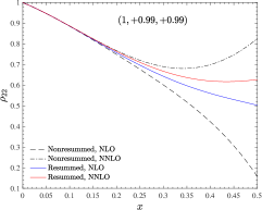
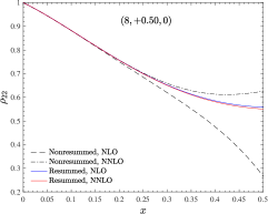
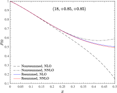
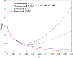
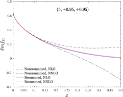
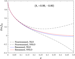
Figure 3: Nonresummed (black) and resummed (colored) waveform amplitudes $\rho_{22}$ (top panels) and $f_{21}$ (bottom panels) for a few configurations. The orbital factor is taken at $3^{+3}$ PN relative accuracy and resummed with the Padé approximants of Table 1. The consistency between NNLO and NLO truncations of the spin terms factor is dramatically improved when the factorization and resummation procedure is applied.

We now proceed by resumming the orbital and spin factors according to the prescriptions of Ref. Nagar and Shah (2016), basically extending to higher modes the treatment of the $\ell=2$ modes discussed there. However, we want to have at least the orbital multipolar factors, $\rho_{\ell m}^{\rm orb}$, consistent with the test-particle ones discussed above, in order to take advantage of the high-order PN-information available and of the robustness of its analytical representation in Padé resummed form. To do so, we follow the, now standard, practice, originally suggested in Ref. Damour et al. (2009), of hybridizing the low-PN-order $\nu$-dependent information available with the high-PN-order test-mass ($\nu=0$) one. At the time of Ref. Damour et al. (2009), the test-particle orbital fluxes were analytically known up to 5.5PN order, which implied that the, nonresummed, $\rho_{\ell m}$’s functions were available as polynomials of different order, that is $\rho_{22}^{\rm orb}=1+x+....+x^{5}$, $\rho_{21}^{\rm orb}=1+x+....+x^{4}$ etc., consistent with the global 5.5PN accuracy of the total flux. This prompted, at the time, the construction of what was called the $3^{+2}$ PN approximation, where the 3PN results were hybridized with two more test-particle PN orders. As we saw above, the availability of PN results of high order Fujita (2012) allows us to keep more PN terms in each $\rho_{\ell m}^{\rm orb}$’s, notably up to 6PN relative accuracy for each $(\ell,m)$ as a good compromise between simplicity and accuracy. Since we are working with relative PN truncations, we give here the $3^{+3}$ PN approximation for the $\rho_{\ell m}(x;\nu)$ a different meaning with respect to Damour et al. (2009). More precisely, working at $3^{+3}$PN order here means that each $\rho_{\ell m}^{\rm orb}(x;\nu)$ carries the complete test-mass information up to $x^{6}$, but whenever possible, the lower PN terms are augmented by the corresponding $\nu$-dependent information compatible with the $\nu$-dependent 3PN accuracy. For example, $\rho_{22}^{\rm orb}(x;\nu)$ formally reads

$$\rho_{22}^{\rm orb}(x;\nu) =1+c_{1}(\nu)x+c_{2}(\nu)x^{2}+c_{3}(\nu;\log(x))x^{3}$$

$$+c^{0}_{4}(\log(x))x^{4}+c^{0}_{5}(\log(x))x^{5}$$

$$+c^{0}_{6}(\log(x),\log^{2}(x))x^{6},$$ (66)

where $(c^{0}_{4},c^{0}_{5},c_{6}^{0})$ are test-particle, $\nu$-independent, coefficients with the corresponding dependence on $\log(x)$. The function $\rho^{\rm orb}_{21}(x;\nu)$ shares the same analytical structure, though the $\nu$-dependence of $c_{3}$ is currently uknown, since it is a (global) 4PN effect. For higher modes, the $\nu$ dependence is progressively reduced, up to only $c_{1}(\nu)$ for the $\ell=8$ modes Damour et al. (2009). Choosing the above defined $3^{+3}$ PN approximation also means that we adopt the same Padé resummation, multipole by multipole, detailed in Table 1. In this way we implement, by construction, the consistency with the $\nu=0$ limit. This choice opens the question of what would be the magnitude of the systematic error done by neglecting such, yet-uncalculated, $\nu$-dependent terms. Reference Damour et al. (2009) analyzed the $\nu$-dependence of a few multipoles and concluded that, working with Taylor-expanded $\rho_{\ell m}^{\rm orb}$, the $\nu$-dependence is mild and that the effect of the missing terms is small enough to be considered of no importance. We shall repeat and update that reasoning to our current choices in the next section, though we anticipate the same conclusion of Damour et al. (2009) remains essentially true here for all examined modes.

We turn now to discussing the resummation of the spinning factors, $\hat{\rho}_{\ell m}^{\rm S}$ and $\hat{f}_{\ell m}^{\rm S}$. We do so by applying the resummation recipe of Ref. Nagar and Shah (2016), that is: (i) for even-$m$, we simply resum $\hat{\rho}_{\ell m}^{\rm S}$ taking its inverse Taylor representation, $\bar{\rho}_{\ell m}^{\rm S}(x;\,\nu)$, as in Eq. (6); (ii) for odd-$m$, we need to resum separately the two factors $\hat{f}^{\rm S_{(0)}}_{{\ell m}}$ and $\hat{f}^{\rm S_{(1)}}_{{\ell m}}$. The analytical representation of the two factors we choose depend on the multipole. More precisely: the factor $\hat{f}_{21}^{\rm S_{(0)}}$ is always resummed taking its inverse Taylor representation. The same choice is also adopted to resum $\hat{f}_{{\ell m}}^{\rm S_{(1)}}$ for $\ell=2$, but for $\ell\geq 3$, $m={\rm odd}$ case, the $\hat{f}_{{\ell m}}^{\rm S_{(1)}}$ are kept in Taylor-expanded form because of the presence of spurious poles when taking the inverse. The quality of the resummation is assessed in Figs. 3 and 4 for a few illustrative binary configurations. Since one does not have at hand the analogous of the test-mass numerical data for circularized, comparable-mass, binaries to compare with, our aim here is only limited to prove the internal consistency of the resummed analytical expressions once taken at different PN orders. To do so, by keeping the orbital part unchanged, we contrast the functions obtained using the full NNLO information with the ones truncated at NLO accuracy. The same figures also display the standard representation of the $\rho_{\ell m}$’s, where no additional factorization or resummation is adopted Pan et al. (2011). The plot illustrates how the spread between the NLO and NNLO truncations in PN-expanded form is systematically much larger than the corresponding one obtained with the factorized and resummed functions. Interestingly, this conclusion remains true for any configuration analyzed. This makes us conclude that factorizing and resumming as discussed here is helpful also in the comparable-mass case, although a precise quantification of the improvement brought by this procedure should be assessed through a comprehensive comparison between an EOB model built from iResum waveforms and NR data, in a way analogous, though more detailed, to what briefly analyzed in Nagar and Shah (2016). However, to better grasp the meaning of this result, it is useful to remind the reader that the merger of a binary black-hole coalescence (defined as the peak of the $\ell=m=2$ waveform amplitude) will occur at $x\approx 0.3$, with $x=(\omega_{22}/2)^{2/3}$ and $\omega_{22}$ the quadrupolar GW frequency. As Figs. 3 and 4 illustrate, the improvement in the consistency between PN truncations brought by the resummation is evident precisely in a neighborhood of $0.3$. Just to pick some random examples, this is the case for $(1,+0.99,+0.99)$ and $(8,+0.50,0)$, configurations where the frequency parameter at merger is $x\approx 0.38$ and $x\approx 0.32$ respectively SXS .

V.1 Mild dependence of $\rho_{\ell m}^{\rm orb}$ to uncalculated $\nu$-dependent orbital terms

As mentioned above, the idea of hybridizing test-mass orbital information with the $\nu\neq 0$ one in the waveform amplitudes dates back to Ref. Damour et al. (2009). The rationale behind that choice was to show that the dependence on $\nu$ of the coefficients in the $\rho_{{\ell m}}^{\rm orb}$ is mild when $0\leq\nu\leq 1/4$, so that one does not introduce a large systematical error in neglecting it. To get to this conclusion, one was comparing the fractional variation of the coefficients when $\nu$ is varied between $0$ and $1/4$ (see Sec. IVA in Damour et al. (2009)). Here we follow the same approach and compute the fractional variation in $\nu$ for all multipoles up to $\ell=6$. The 3PN-accurate $\nu$-dependent terms in $\rho^{\rm orb}_{31}$ and $\rho^{\rm orb}_{33}$ that were obtained only in Ref. Faye et al. (2015) are also included. The $\log(x)$ terms are evaluated, for simplidicty at $x_{\rm LSO}^{\rm Schw}=1/6$. The numbers listed in Table 2 suggest that, up to $\ell=3$, the next missing $\nu$-dependent term might be, on average, of the order of $20\%$ larger (or smaller) then the test-mass ($\nu=0$) one (note however the larger variations of the 2PN coefficient in $\rho_{31}^{\rm orb}$ and $\rho_{32}^{\rm orb}$. One can then investigate the impact on $\rho_{\ell m}^{\rm orb}$ of missing $\nu$-dependent corrections by varying the $\nu=0$ term by $\pm 30\%$. Clearly, the operation has to be done on the $P^{m}_{n}(\rho^{\rm orb}_{\ell m})$ function. To be concrete on one case, let us analyze the effect on $\rho_{21}^{\rm orb}$, whose known $\nu$-dependence stops at 2PN. Schematically, the Taylor-expanded function reads

$$\rho_{21}^{\rm orb}=1+(c^{\rm 1PN}_{0}+c^{\rm 1PN}_{\nu})x+(c^{\rm 2PN}_{0}+c_{\nu}^{\rm 2PN})x^{2}$$

$$+\left[c^{\rm 3PN}_{0}(1+\alpha)\right]x^{3}+c_{0}^{\rm 4PN}x^{4}+c_{0}^{\rm 5PN}x^{5}+c_{0}^{\rm 6PN}x^{6},$$ (67)

and then one takes its $P^{5}_{1}$ Padé approximant. Here, $c_{0}^{n\rm PN}$ indicate the $\nu=0$ coefficients, while $c_{\nu}^{n\rm PN}$ the corresponding $\nu$-dependent terms. The effect of the missing $\nu$-dependent information is parametrized through $\alpha$. One finds that, even putting $\alpha=\pm 0.20$ with $\nu=1/4$, the fractional variation in $P^{5}_{1}\left(\rho_{21}^{\rm orb}\right)$ is of the order of $0.04\%$ at the Schwarzschild LSO $x_{\rm LSO}^{\rm Schw}=1/6$, of the order of $0.9\%$ at $x=1/3$ and of the order of $6\%$ at $x=1/2$. This value is close to the LSO location of a Kerr black hole with $\hat{a}=+0.99$ and we use here just for illustrative purposes, since a comparable mass binary, with a nonnegligible value of $\nu$, is not expected to reach such a high frequency at merger. Since the waveform amplitude is just $(\rho_{21})^{2}$, the fractional differences above get a factor two in front, which suggests that, within the current framework, one is expecting the 3PN correction to $\rho_{21}^{\rm orb}$ to yield an amplitude correction around merger of just a few percents. Once the calculation of the waveform will be completed at 4PN accuracy Damour et al. (2016); Marchand et al. (2016); Damour and Jaranowski (2017); Marchand et al. (2017); Bernard et al. (2017), it will be interesting to concretely probe the reasonable assumptions we are adopting here. In addition, inspection of the behavior of higher modes, like $\rho_{44}^{\rm orb}$, shows that a variation of the order $20\%$ with respect to the $\nu=0$ values has an unnaturally large effect on the global behavior of the function in the strong-field regime ($0.3\lesssim x\lesssim 0.5$), with variations of order $8\%$ at $x=1/3$ and $\sim 30\%$ at $x=1/2$. Though we cannot make strong statements, we are prone to think that the uncalculated $\nu$-dependent terms will provide, on average, a correction of the order of $10\%$ to the current orbital terms, consistently with the $\nu$-variation of the 3PN coefficients in $\rho^{\rm orb}_{22}$ and $\rho_{33}^{\rm orb}$, as in Table 2.

Table 2: Analysis of the fractional variation $\triangle c_{n}^{\rho_{\ell m}^{\rm orb}}(\nu)=c_{n}^{\rho_{\ell m}^{\rm orb}}(\nu)/c_{n}^{\rho_{\ell m}^{\rm orb}}(0)-1$ of the coefficients $c_{n}^{\rho_{\ell m}^{\rm orb}}(\nu)$.

$(\ell,m)$	$\triangle c_{1}^{\rho_{\ell m}^{\rm orb}}(1/4)$	$\triangle c_{2}^{\rho_{\ell m}^{\rm orb}}(1/4)$	$\triangle c_{1}^{\rho_{\ell m}^{\rm orb}}(1/4,\log(1/6))$
$(2,2)$	-0.159884	0.185947	-0.100421
$(2,1)$	-0.649718	0.224005	…
$(3,1)$	0.0769231	-18.7351	-0.28487
$(3,2)$	-0.155488	-0.633264	…
$(3,3)$	-0.142857	0.260344	-0.0970255
$(4,1)$	-0.0905316	…	…
$(4,2)$	-0.0181065	1.05237	…
$(4,3)$	-0.141892	…	…
$(4,4)$	-0.230328	0.46265	…
$(5,1)$	0.219436	…	…
$(5,2)$	-0.117576	…	…
$(5,3)$	-0.0746667	…	…
$(5,4)$	-0.176295	…	…
$(5,5)$	-0.201232	…	…
$(6,1)$	-0.0910973	…	…
$(6,2)$	-0.0168919	…	…
$(6,3)$	-0.118343	…	…
$(6,4)$	-0.119186	…	…
$(6,5)$	-0.165766	…	…
$(6,6)$	-0.238208	…	…

V.2 Hybridizing test-mass results: the spin information

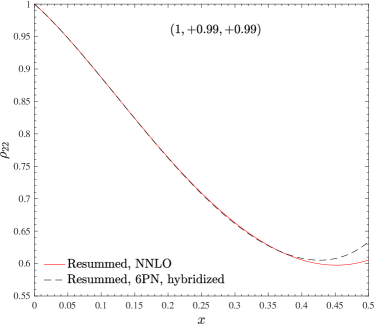
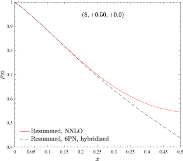
Figure 5: Modification of the results of Fig. 3 when (nonspinning) test-particle terms up to 6PN are hybridized with the NNLO $\nu$-dependent waveform (see Eqs. (V.2)-(V.2) and text). When $\nu=0$, one is using here the same spin-orbit and spin-square analytical information used in Fig. (1). The frequency parameter approximately corresponding to the BBH merger is $x\approx 0.38$ for $(1,+0.99,+0.99)$ and $x\approx 0.32$ for $(8,+0.50,0)$. In this latter case, the effect of the additional test-particle terms is important towards merger.

Now that we have justified our approach of hybridizing $\nu=0$ and $\nu\neq 0$ information in the $\rho_{\ell m}^{\rm orb}$ functions, one wonders whether an analogous procedure exits for the $\rho^{\rm S}_{\ell m}$ (and in turn for the factorized $\hat{\rho}_{\ell m}^{\rm S}$). This would allow to have EOB waveforms fully consistent and complete all over the parameter space of nonprecessing BBHs . Such hybridization is rather straightforward to do by taking advantage of the structure of the $\rho_{\ell m}^{\rm S}$ and $f_{\ell m}^{\rm S}$ functions and understanding how the spinning test-particle limit builds up. This is especially evident using the $\tilde{a}_{i}$ variables, that make the limit look apparent. To explain the approach, let us first focus on the spin-orbit terms entering the $\rho_{\ell m}$ functions. One sees that, at a given $n$-PN order of the orbital part, the corresponding spin-orbit term reads like

$$\Bigg{(}\hat{a}_{0}(c_{0}+c_{1}\nu+\dots+c_{n-1}\nu^{n-1})$$

$$+\tilde{a}_{12}X_{12}(d_{0}+d_{1}\nu+\dots+d_{n-1}\nu^{n-1})\Bigg{)}x^{(2n+1)/2},$$ (68)

as it is clear from Eq. (39) that corresponds to 3PN orbital dynamics. Note that within our writing, the LO spin-orbit coefficients are $\nu$-independent, the NLO are linear in $\nu$, while the NNLO are quadratic in $\nu$. A similar, though slightly more complicated, structure is found for the quadratic-in-spin terms, that, e.g. for $\rho_{22}^{\rm S}$, are given as the sum of terms proportional to $\hat{a}_{0}^{2}$, $\tilde{a}_{1}\tilde{a}_{2}$ and $\hat{a}_{0}\tilde{a}_{12}X_{12}$. As for the SO case above, at LO there is no $\nu$ dependence, while it is similarly linear-in-$\nu$ at NLO. The $\nu$ independent terms in Eq. (39) are those that, combined together when $\nu\rightarrow 0$, generate the (spinning) test particle results, see e.g. Refs. Tanaka et al. (1996); Fujita (2015). Understood this, one can implement the inverse process, namely incorporate the $\rho^{\rm S}_{\ell m}$’s (and $f_{\ell m}^{\rm S}$) obtained from the perturbative calculations of the fluxes of a spinning particle around a Kerr black hole by imposing the structure given by Eq. (V.2). This means, in particular, replacing the dimensionelss Kerr spin as $\hat{a}\rightarrow\tilde{a}_{1}$ and the particle spin as $\sigma\rightarrow\tilde{a}_{2}$. In other words, on the $\nu$-dependent side, the next-to-next-to-next-to-leading-order (NNNLO) spin-orbit term will have the form

$$c_{22}^{\rm SO^{\rm NNNLO}_{\nu}}=\left(c_{0}^{\rm NNNLO}\hat{a}_{0}+X_{12}\tilde{a}_{12}d_{0}^{\rm NNNLO}\right)x^{9/2},$$ (69)

where $\left(c_{0}^{\rm NNNLO},d_{0}^{\rm NNNLO}\right)$ are the unknown $\nu$-independent, coefficients. On the $\nu=0$ side, the corresponding spin-orbit terms reads

$$c_{22}^{\rm SO_{0}^{\rm 4.5PN}}=\left(c_{\hat{a}}^{\rm 4.5PN}\hat{a}+c_{\sigma}^{\rm 4.5PN}\sigma\right)x^{9/2}.$$ (70)

By equationg the $\nu=0$ limit of Eq. (70) to this equation, one finds

$$c_{22}^{{\rm SO}^{\rm NNNLO}_{\nu}} =\Bigg{(}\dfrac{c_{\hat{a}}^{\rm 4.5PN}+c_{\sigma}^{\rm 4.5PN}}{2}\hat{a}_{0}$$

$$\qquad+X_{12}\tilde{a}_{12}\dfrac{c_{\hat{a}}^{\rm 4.5PN}-c_{\sigma}^{\rm 4.5PN}}{2}\Bigg{)}x^{9/2},$$ (71)

where $c_{\hat{a}}^{\rm 4.5PN}$ is analytically known Fujita (2015) and reads

$$c_{\hat{a}}^{\rm 4.5PN}=-\dfrac{8494939}{467775}+\dfrac{2536}{315}{\rm eulerlog}_{2}(x),$$ (72)

while the spinning-particle term, $c_{\sigma}^{\rm 4.5PN}$, is currently unknown. The same procedure can be applied to incorporate spinning-particle spin-orbit terms at higher-PN order and can be extended to the other multipoles, with the obvious difference that for $m$-odd multipoles the hybridization procedure applies to the $f_{\ell m}^{\rm S}$ functions. The hybridization of the spinning-particle, spin-square terms into $\rho_{22}^{\rm S}$ is done in a similar way. A similar calculation for the NNLO ( relative 4PN-accuracy) spin-square term yields

$$c_{22}^{\rm SS^{NNLO}_{\nu}} =\Bigg{[}\dfrac{1}{2}\left(c_{\hat{a}^{2}}+c_{\sigma^{2}}\right){\hat{a}}_{0}^{2}+\left(c_{{\hat{a}}\sigma}-c_{{\hat{a}}^{2}}-c_{\sigma^{2}}\right)\tilde{a}_{1}\tilde{a}_{2}$$

$$+\dfrac{1}{2}\left(c_{{\hat{a}}^{2}}-c_{{\sigma}^{2}}\right)\hat{a}_{0}\tilde{a}_{12}X_{12}\Bigg{]}x^{4},$$ (73)

where $(c_{\sigma^{2}},c_{{\hat{a}}\sigma},c_{\sigma^{2}})$ are the coefficients entering the spin-square spinning-particle term at 4PN, that will have the structure

$$c_{22}^{\rm SS_{0}}=\left(c_{{\hat{a}}^{2}}{\hat{a}}^{2}+c_{{\hat{a}}\sigma}{\hat{a}}\sigma+c_{\sigma^{2}}\sigma^{2}\right)x^{4},$$ (74)

where only $c_{{\hat{a}}^{2}}$ is currently analytically known and reads Fujita (2015)

$$c_{{\hat{a}}^{2}}=\dfrac{18353}{21168}.$$ (75)

This approach gives us a consistent way of hybridizing the test-mass result above with the low-PN $\nu$-dependent information. Even if the spinning-particle terms are not currently published starting from 4PN order, it could be instructive to investigate the robustness of the results of Fig. 3 under the incorporation of the nonspinning test-particle terms. To do so, we replicate the procedure done above to incorporate the 4PN and 4.5PN test-particle terms for the spin-square 5PN and 6PN terms as well as for the 5.5PN spin-orbit term, that will have the same relation given in Eqs. (69)-(V.2) with the test-particle coefficients. After this is done, we factorize and resum the hybrid $\rho_{22}$ as before. Such, test-particle-improved, $\bar{\rho}^{\rm S}_{22}$ is consistent with the $\nu=0$ function discussed in Sec. II except for the obvious absence of the spin-cube terms coming beyond the NLO as well as of the terms involving higher powers of the spins up to the sixth-power, that enters at LO in the 6PN term. The effect of the additional $\nu=0$ terms is illustrated in Fig. 5 for $(1,+0.99,+0.99)$ and $(8,+0.50,0)$, where the hybridized function is contrasted with the NNLO one of Fig. 3. The figure shows that the effect is quantitatively important for the case $(8,+0.50,0)$, notably towards the merger freuquency $x\approx 0.32$. We postpone to future work a deeper study of the effect of the $\nu=0$ terms all over the parameter space and of their importance in comparisons with NR waveform data. Such study will be performed by including also some of the higher-order spin-orbit terms for a circularized spinning particle that are currently not available in the literature and that are being calculated Kavanagh et al. (2018).

VI Conclusions

In this paper we have improved and generalized the factorization and resummation procedure of waveform amplitudes introduced in Ref. Nagar and Shah (2016). The key conceptual step of the approach relies on factorizing the orbital and the spin-dependence into two separate factors that can then be resummed separately in various ways. Our results can be summarized as follows:

• Concerning a circularized, (nonspinning) particle orbiting a Kerr black hole, we have shown that the (relative) 6PN-accurate $\rho_{\ell m}$ functions can be factorized and resummed in a form that yields a more than satisfactory agreement (of the order of a few $\%$) with the corresponding numerical (exact) function up to the last-stable-orbit. This is notably true for the case of a quasi-extremal black hole with dimensionless spin parameter $\hat{a}=+0.99$. One of the novelties with respect to previous work Nagar and Shah (2016) is that the 6PN-accurate orbital function $\rho_{22}^{\rm org}$ is resummed with a Padé approximant (typically $P^{4}_{2}$). The same recipe proved to work essentially the same way for all subdominant modes up to $\ell=6$, modulo a few exceptions where working at either higher or lower PN-information proved a better choice 1). More concretely, the factorization-resummation procedure allows us to obtain an analytic flux, summed over all multipoles up to $\ell=6$, that is consistent at the $5\%$ fractional level up to the LSO, for the most demanding case of $\hat{a}=+0.99$. This result is accomplished relying only on purely analytical information, without any additional fit to the numerical fluxes. We recall that this route was followed instead in Ref. Taracchini et al. (2013) , where several higher-PN terms, unknown at the time, were calibrated to the same Teukolsky data we are using here. The fits were able to improve the standard $\rho_{\ell m}$-nonresummed flux so to have a fractional difference at the LSO of the order (or below) $1\%$. We have briefly illustrated (for the $\ell=m=2$ mode only, see end of Sec. II) that an analogous route can be followed also in our framework and that it is easy to reach analytical/numerical fractional differences in $\rho_{22}$ of the order of $0.1\%$ at the LSO for $\hat{a}=+0.99$ by just choosing one effective parameter entering at 6.5PN order in the resummed spin factor $\bar{\rho}_{22}^{\rm S}$. Alternatively, we want to remind that we have explored only a few of the many possibile choices. Focusing on the $(2,2)$ mode only for definitess, the logic driving our approach is: first (i), to simplify things we choose to keep the same PN-order for both the orbital and PN factors; then (ii), as a similarly simple choice to reduce the growth of the spin factor in the strong-field regime (see discussion in Ref. Nagar and Shah (2016)), we resummed it with its inverse-Taylor approximant; (iii) finally, we found that a good match with the exact numerical data was found by taking the $P^{4}_{2}$ Padé approximant of the orbital factor. Once the factorization paradigm is accepted, any of the points (i)-(iii) above could be, in principle, changed. For example, for $(3,1)$ we found that the numerical/analytical agreement gets improved by keeping the spin factor at 8PN accuracy and the orbital factor just at 4PN accuracy resummed with a $(3,1)$ Padé approximant. Similarly, for some multipoles like $(3,3)$ and $(4,4)$ things are such that the straight, Taylor-expanded, form of the orbital factor yields a better agreement with the numerical results. These facts suggest that it might be possible that there are some special combinations of Padé approximant for the orbital part and PN-truncation of the spin factor that could further reduce the analytical/numerical disagreement in the near-LSO regime. Seen the large amount of PN-knowledge that is available (up to 20PN Shah (2014)), this would require a specific, dedicated study depending on the spin regime where one would like to use the resummed flux. For example, the resummed analytical fluxes we present here could be use to improve the radiation reaction force used to drive the quasi-circular transition from inspiral to plunge in the test-particle limit Harms et al. (2014). Several studies showed the limits of the standard, nonresummed, analytical approach at 5PN Harms et al. (2014) and proposed to improve it with effective fits Taracchini et al. (2013). The approach we present here offers an alternative, though slightly less accurate, to the effective fits of Taracchini et al. (2013). Whether such difference is relevent or not will depend on the specific configuration and/or the problem under consideration. For example, it will be interesting to investigate to which extent the perturbative calculation of the recoil velocity of Ref. Harms et al. (2014) can be improved by the use of the new radiation reaction presented here, in particular when the central Kerr black hole is quasi-extremal with spin aligned with the orbital angular momentum.

• . We have extended the factorization and resummation procedure to all the existing $\nu$-dependent spin terms. This means that we go up to NNLO in the spin-orbit coupling, up to NLO in the spin-spin coupling and up to LO in the spin-cube coupling. This is done consistently for all multipoles currently known above the LO contributions ($\ell=4$). In doing so, we propose to use the orbital part of the waveform in hybridized form, where currently known, $\nu$-dependent orbital terms are hybridized with the test-mass term, as proposed long ago in Damour et al. (2009). The novelty here is that, to maintain the consistency with the choices done in the test-particle limit, each $\rho_{{\ell m}}$ is kept up to relative 6PN order (but a few exceptions), with the Padé-approximant that was chosen in the test-particle limit, however maintaining the full $\nu$-dependence that is currently available in the low-order terms. By contrast, as a first choice, the spin-dependent factor is not hybridized with high-order test-particle results, but it is inverse resummed at the currently available $\nu$-dependent PN order. We have explored the robustness of this choice on an indicative sample of binary configurations, contrasting the resummed amplitude with the plain, Taylor-expanded, $\rho_{\ell m}$. Since we do not have circularized comparable-mass BH data to compare with, the only effect that we could investigate for is the consistency between NNLO and NLO truncations of the waveform, as an indication of the analytical robustness of the resummed expressions. Our Figs. 3 (for $\ell=2$) and 4 (for $\ell=3$) show that, for the same binary, differences that are large for the Taylor-expanded $\rho_{\ell m}$ or $\delta mf_{\ell m}$ are either very much reduced, or practically negligible, in the resummed representation of the same functions. This effect is very striking on $\delta mf_{21}$, where not only one can see this effect, but the function is also qualitatively close to the numerical one (see for example Fig. 5 of Ref. Nagar and Shah (2016).

  These findings suggest that the resummed waveform amplitudes should be incorporated within the EOB approach as a new, state-of-the-art, analytical waveform paradigm. This was pointed out already in Ref. Nagar and Shah (2016), but here we reinforce that statement after a deeper and more detailed analysis. In particular, we expect that next-to-quasi-circular corrections Damour and Nagar (2007) to the waveforms will generically have a smaller impact than in current EOB models Nagar et al. (2017), because they will hopefully have to bring just small corrections to the already good strong-field behavior of the analytical waveform. This was briefly pointed out already in Ref. Nagar et al. (2017), but we are planning to investigate this extensively in future work.

  (iii) Following Ref. Nagar and Shah (2016), we wrote all spin-dependent expressions using as spin variables the Kerr parameters of the individual black holes divided by the total mass of the system, $\tilde{a_{i}}\equiv a_{i}/M=S_{i}/(m_{i}M)$. The use of this quantities to parametrize a spin-dependent function was already suggested in Ref. Nagar et al. (2016) in the context of informing a next-to-next-to-next-to-leading order spin-orbit effective parameter using NR simulations; similarly, the same spin variables allow for a simple recasting of the NLO correction to the centrifugal radius, that has rather complicated coefficients when written using the dimensionless spin variables $\chi_{i}=S_{i}/m_{i}^{2}$, see Eq. (58)-(65) of Nagar et al. (2016). When using $\tilde{a}_{i}$, Eq. (58) of Nagar et al. (2016) reduces to the following very compact form

  $$\delta a^{2} =\dfrac{M}{r^{3}}\bigg{\{}\dfrac{5}{4}\tilde{a}_{12}\hat{a}_{0}X_{12}-\left(\dfrac{5}{4}+\dfrac{\nu}{2}\right)\hat{a}_{0}^{2}$$

  $$\qquad\quad+\left(\dfrac{1}{2}+2\nu\right)\tilde{a}_{1}\tilde{a}_{2}\bigg{\}}.$$ (76)

  The use of the $\tilde{a}_{i}$’s in our context, on top of providing similar simplifications in writing the formulas, is extremely convenient since these variables are natuarally connected to the (spinning) test-particle limit, that can be obtained straightforwardly by just putting $\nu=0$ in the equations. On top of this, since our analytical writing of the fluxes makes absolutely transparent which terms combine to generate the (spinning) test-particle limit, it is technically clear how to hybridize the $\nu=0$ information with $\nu\neq 0$ one also in the presence of spin, in order to have a waveform model that is fully consistent with the test-mass results discussed at point (i) above. This analysis suggests then that, since the structure of the expansion of the functions $\rho_{22}^{\rm S}$ (or $\hat{\rho}_{22}^{\rm S}$) is clear, one can have access to the leading-order, $\nu$-independent terms, by using perturbative, spinning, test-particle analytical calculations Tanaka et al. (1996); Fujita (2015) and then promoting the BH dimensionless spin $\hat{a}=S_{1}/m_{1}^{2}$ to $\tilde{a}_{1}$ and the spin of the particle $\sigma=S_{2}/(m_{1}m_{2})$ to $\tilde{a}_{2}$, though keeping the additional constraint that a special structure with $X_{12}\tilde{a}_{12}$ exists in the $\nu$-dependent case. This constraint implies that the $\nu$-independent terms entering $\rho_{\ell m}(x;\nu)$ are obtained as linear combinations of the spinning and nonspinning test-particle perturbative results. Unfortunately, since the current accuracy of the fluxes of a spinning-particle obtained using perturbative calculations is still at 2.5 PN order Tanaka et al. (1996), currently we can only rely on nonspinning test-particle perturbative to explore the effect of the hybridization. As a preliminary analysis, focusing only on the $(2,2)$ mode, we hybridized the (nonspinning) particle ($\nu=0$) spin-orbit and spin-spin analytical information on a Kerr black hole up to 6PN with the $\nu$-dependent analytical pieces up to NNLO in the spin-orbit coupling (i.e., 3.5PN). The modifications we found for large values of $x$ are quantitatively more important when the mass-ratio is large than for the equal-mass case, see Fig. (5). However, since the spinning-particle information is not incorporated, since $c_{\sigma}=c_{\sigma^{2}}=c_{\hat{a}\sigma}=0$ for all higher PN orders considered, this result should be taken only as illustrative of the effect and of the general strategy that might be used to take into account spinning $\nu=0$ information. Deeper analytical explorations are necessary to understand whether the test-mass information should be incorporated in this form in current EOB waveform models and whether it is of any help/relevance for LIGO/Virgo sources. In this respect it will be extremely useful to have perturbative analytical calculation of the energy fluxes emitted by a spinning particle on circular orbits around a Schwarzschild (or even a Kerr) black hole, a work that is currently in progress Kavanagh et al. (2018). In the former case, for instance restricted to the simpler case of working at linear order in the particle’s spin, we could already complement the current $\nu=0$ spin-orbit knowledge, and possibly improve, in a more consistent way, the analysis sketched in Fig. 5. In addition, the fluxes of a spinning particle on Kerr would give us access to some leading-order $\tilde{a}_{1}\tilde{a}_{2}$ terms. Though stating whether such test-particle information will have any important impact on LIGO/Virgo targeted waveform models requires deeper investigations, it will certainly allow us to improve their self-consistency all over the binary parameter space.

Appendix A Multipolar fluxes

In this Appendix we explicitly report, for completeness, the PN-expanded, complete, Newton-normalized multipoles of the energy flux up to NNLO in the spin-orbit coupling, NLO in the spin-spin coupling and LO in the spin-cube couplings. Though these expressions are obtained as the square of the Newton-normalized waveform multipoles of Eqs. (III.1)-(24), it is convenient to have them written down explicitly. Each multipolar contribution to the flux is written as the product of the Newtonian prefactor $F_{\ell m}^{N}$ and the PN correction $\hat{F}_{\ell m}$ as

$$F_{\ell m}\equiv F_{\ell m}^{(N,\epsilon)}\hat{F}_{\ell m}^{(\epsilon)},$$ (77)

where the PN correction factors explicitly read

$$\hat{F}_{22}^{(0)} =1+\left(-2{\hat{a}}_{0}+4\pi-\frac{2}{3}{\tilde{a}}_{12}X_{12}\right)x^{3/2}+\left(-\frac{107}{21}+\frac{55}{21}\nu\right)x+\left(\frac{4784}{1323}+2{\hat{a}}_{0}^{2}-\frac{87691}{5292}\nu+\frac{5851}{1323}\nu^{2}\right)x^{2}$$

$$+\biggl{[}\left(-\frac{428}{21}+\frac{178}{21}\nu\right)\pi+{\hat{a}}_{0}\left(\frac{158}{63}-\frac{257}{63}\nu\right)-{\tilde{a}}_{12}X_{12}\left(\frac{50}{63}+\frac{187}{63}\nu\right)\biggr{]}x^{5/2}$$

$$+\biggl{[}\frac{99210071}{1091475}+\frac{1650941}{349272}\nu-\frac{669017}{19404}\nu^{2}+\frac{255110}{43659}\nu^{3}+\left(\frac{16}{3}+\frac{41}{48}\nu\right)\pi^{2}$$

$$-\left(8{\hat{a}}_{0}+\frac{8}{3}{\tilde{a}}_{12}X_{12}\right)\pi+\frac{257}{63}\nu\left({\tilde{a}_{1}}^{2}+\frac{962{\tilde{a}_{1}}{\tilde{a}_{2}}}{257}+{\tilde{a}_{1}}^{2}\right)+\frac{284}{63}X_{12}\left({\tilde{a}_{1}}^{2}-{\tilde{a}_{2}}^{2}\right)$$

$$-\frac{53}{7}\left({\tilde{a}_{1}}^{2}+\frac{1072{\tilde{a}_{1}}{\tilde{a}_{2}}}{477}+{\tilde{a}_{2}}^{2}\right)-\frac{1712}{105}{\rm eulerlog}_{2}(x)\biggr{]}x^{3}$$

$$+\biggl{[}\left(\frac{19136}{1323}-\frac{144449}{2646}\nu+\frac{33389}{2646}\nu^{2}\right)\pi+{\hat{a}}_{0}\left(\frac{29234}{1323}+\frac{77212}{1323}\nu+\frac{1747}{1323}\nu^{2}\right)$$

$$+{\tilde{a}}_{12}X_{12}\left(\frac{37858}{3969}+\frac{96575}{7938}\nu-\frac{23182}{3969}\nu^{2}\right)-\frac{2}{3}({\hat{a}}_{0}^{3}+3{\hat{a}}_{0}^{2}{\tilde{a}}_{12}X_{12})\biggr{]}x^{7/2},$$ (78)

$$\hat{F}_{21}^{(1)} =1-4\nu-3{\tilde{a}}_{12}X_{12}x^{1/2}+\left(-\frac{17}{14}+\frac{44}{7}\nu-\frac{40}{7}\nu^{2}+\frac{9}{4}{\tilde{a}}_{12}^{2}\right)x+\biggl{[}2\pi(1-4\nu)+{\hat{a}}_{0}\left(-\frac{43}{7}+\frac{172}{7}\nu\right)$$

$$+{\tilde{a}}_{12}X_{12}\left(\frac{195}{28}+\frac{18}{7}\nu\right)\biggr{]}x^{3/2}+\biggl{\{}-\frac{2215}{7056}-\frac{13567}{1764}\nu+\frac{65687}{1764}\nu^{2}-\frac{853}{147}\nu^{3}$$

$$-\frac{26}{7}\left({\tilde{a}_{1}}^{2}-\frac{68}{13}{\tilde{a}_{1}}{\tilde{a}_{2}}+{\tilde{a}_{2}}^{2}\right)-\frac{323}{14}\left({\tilde{a}_{1}}^{2}+\frac{26}{323}{\tilde{a}_{1}}{\tilde{a}_{2}}+{\tilde{a}_{2}}^{2}\right)\nu+X_{12}\biggl{[}\frac{157}{14}({\tilde{a}_{1}}^{2}-{\tilde{a}_{2}}^{2})-6\pi{\tilde{a}}_{12}\biggr{]}\biggr{\}}x^{2}$$

$$+\biggl{\{}\left(\frac{9}{2}{\tilde{a}}_{12}^{2}-\frac{17}{7}+\frac{81}{7}\nu-\frac{52}{7}\nu^{2}\right)\pi+{\hat{a}}_{0}\left(\frac{2131}{882}-\frac{1165}{147}\nu-\frac{3068}{441}\nu^{2}\right)$$

$$-{\tilde{a}}_{12}X_{12}\left(\frac{10121}{1764}-\frac{30595}{882}\nu-\frac{16927}{3528}\nu^{2}\right)+3{\hat{a}}_{0}{\tilde{a}}_{12}^{2}+\frac{3}{2}X_{12}[5({\tilde{a}_{1}}^{3}-{\tilde{a}_{2}}^{3})+{\tilde{a}_{1}}({\tilde{a}_{1}}{\tilde{a}_{2}}-{\tilde{a}_{2}}^{2})]\biggr{\}}x^{5/2},$$ (79)

$$\hat{F}_{31}^{(0)} =1-4\nu+\left(-\frac{16}{3}+20\nu+\frac{16}{3}\nu^{2}\right)x+\biggl{[}2\pi(1-4\nu)+{\hat{a}}_{0}\left(\frac{1}{2}-2\nu\right)+{\tilde{a}}_{12}X_{12}\left(-\frac{9}{2}+13\nu\right)\biggr{]}x^{3/2}$$

$$+\biggl{[}\frac{437}{33}-\frac{5164}{99}\nu-\frac{523}{99}\nu^{2}+\frac{812}{99}\nu^{3}+3{\hat{a}}_{0}^{2}(1-4\nu)-8X_{12}({\tilde{a}_{1}}^{2}-{\tilde{a}_{2}}^{2})\biggr{]}x^{2}$$

$$+\biggl{[}\left(-\frac{32}{3}+39\nu+\frac{44}{3}\nu^{2}\right)\pi+{\hat{a}}_{0}\left(-\frac{103}{18}+\frac{283}{6}\nu-\frac{874}{9}\nu^{2}\right)+{\tilde{a}}_{12}X_{12}\left(\frac{145}{6}-\frac{1211}{18}\nu-\frac{41}{3}\nu^{2}\right)\biggr{]}x^{5/2},$$ (80)

$$\hat{F}_{32}^{(1)} =1+\frac{1}{1-3\nu}\biggl{\{}2({\hat{a}}_{0}-{\tilde{a}}_{12}X_{12})x^{1/2}+\left(-\frac{193}{45}+\frac{145}{9}\nu-\frac{73}{9}\nu^{2}\right)x$$

$$+\frac{1}{(1-3\nu)}\biggl{[}4\pi(1-3\nu)^{2}+{\hat{a}}_{0}\left(-\frac{778}{45}+\frac{715}{9}\nu-\frac{730}{9}\nu^{2}\right)+{\tilde{a}}_{12}X_{12}\left(\frac{538}{45}-\frac{313}{9}\nu-\frac{44}{9}\nu^{2}\right)\biggr{]}x^{3/2}\biggr{\}},$$ (81)

$$\hat{F}_{33}^{(0)} =1-4\nu+(-8+36\nu-16\nu^{2})x+\biggl{[}6\pi(1-4\nu)+{\hat{a}}_{0}\left(-\frac{7}{2}+14\nu\right)+{\tilde{a}}_{12}X_{12}\left(-\frac{1}{2}+5\nu\right)\biggr{]}x^{3/2}$$

$$+\biggl{[}\frac{1003}{55}-\frac{18352}{165}\nu+\frac{8937}{55}\nu^{2}-\frac{6188}{165}\nu^{3}+3{\hat{a}}_{0}^{2}(1-4\nu)\biggr{]}x^{2}$$

$$+\biggl{[}(-48+213\nu-84\nu^{2})\pi+{\hat{a}}_{0}\left(\frac{559}{30}-\frac{843}{10}\nu+\frac{586}{15}\nu^{2}\right)+{\tilde{a}}_{12}X_{12}\left(-\frac{59}{30}-\frac{183}{10}\nu+\frac{391}{15}\nu^{2}\right)\biggr{]}x^{5/2}\ ,$$ (82)

$$\hat{F}_{41}^{(1)} =1-4\nu+\frac{1}{-1+2\nu}\biggl{\{}\biggl{[}{\hat{a}}_{0}\left(-\frac{5}{2}+10\nu\right)+{\tilde{a}}_{12}X_{12}\left(\frac{5}{2}-5\nu\right)\biggr{]}x^{1/2}$$

$$+\biggl{[}\frac{202}{33}-\frac{2627}{66}\nu+\frac{2188}{33}\nu^{2}-\frac{664}{33}\nu^{3}\biggr{]}x\biggr{\}}\ ,$$ (83)

$$\hat{F}_{42}^{(0)} =1+\frac{1}{1-3\nu}\biggl{\{}\left(-\frac{1311}{165}+\frac{805}{33}\nu-\frac{19}{11}\nu^{2}\right)x$$

$$+\biggl{[}4\pi(1-3\nu)-\frac{4}{5}{\hat{a}}_{0}\left(\frac{1}{3}-\nu\right)-{\tilde{a}}_{12}X_{12}\left(\frac{76}{15}-\frac{52}{5}\nu\right)\biggr{]}x^{3/2}$$

$$+\frac{1}{(1-3\nu)}\left(\frac{7199152}{275275}-\frac{140762423}{825825}\nu+\frac{37048126}{117975}\nu^{2}-\frac{3504901}{31460}\nu^{3}-\frac{65037}{7865}\nu^{4}\right)x^{2}\biggr{\}},$$ (84)

$$\hat{F}_{43}^{(1)} =1-4\nu+\frac{1}{-1+2\nu}\biggl{\{}\biggl{[}{\hat{a}}_{0}\left(-\frac{5}{2}+10\nu\right)+{\tilde{a}}_{12}X_{12}\left(\frac{5}{2}-5\nu\right)\biggr{]}x^{1/2}$$

$$+\left(\frac{78}{11}-\frac{3139}{66}\nu+\frac{932}{11}\nu^{2}-\frac{1048}{33}\nu^{3}\right)x\biggr{\}},$$ (85)

$$\hat{F}_{44}^{(0)} =1+\frac{1}{1-3\nu}\biggl{\{}\left(-\frac{1779}{165}+\frac{1273}{33}\nu-\frac{175}{11}\nu^{2}\right)x$$

$$+\biggl{[}8\pi(1-3\nu)-{\hat{a}}_{0}\left(\frac{76}{15}-\frac{76}{5}\nu\right)-{\tilde{a}}_{12}X_{12}\left(\frac{4}{15}-\frac{28}{5}\nu\right)\biggr{]}x^{3/2}$$

$$+\frac{1}{(1-3\nu)}\biggl{(}\frac{2187772}{55055}-\frac{261025727}{825825}\nu+\frac{95748634}{117975}\nu^{2}-\frac{4466169}{6292}\nu^{3}+\frac{1119423}{7865}\nu^{4}\biggr{)}x^{2}\biggr{\}}.$$ (86)

The Newtonian prefactor can be written in closed form as

$$F^{(N,\epsilon)}_{\ell m}=\dfrac{1}{8\pi}x^{3}m^{2}(-)^{\ell+\epsilon}\left|{\cal R}h_{\ell m}^{(N,\epsilon)}\right|^{2}\ ,$$ (87)

where the Newtonian waveform multipole $h_{\ell m}^{(N,\epsilon)}$ is explicitly given as Damour et al. (2009)

$${\cal R}h_{\ell m}^{(N,\epsilon)}=M\nu\,n_{\ell m}^{(\epsilon)}c_{\ell+\epsilon}(\nu)x^{(\ell+\epsilon)/2}Y_{\ell-\epsilon,-m}(\pi/2,\phi)\ ,$$ (88)

with

$$c_{\ell+\epsilon}(\nu)=X_{2}^{\ell+\epsilon-1}+(-)^{\ell+\epsilon}X_{1}^{\ell+\epsilon-1}$$ (89)

and

$$n_{\ell m}^{(0)} =({\rm i}m)^{\ell}\dfrac{8\pi}{(2\ell+1)!!}\sqrt{\dfrac{(\ell+1)(\ell+2)}{\ell(\ell-1)}}\ ,$$ (90)

$$n_{\ell m}^{(1)} =-({\rm i}m)^{\ell}\dfrac{16\pi{\rm i}}{(2\ell+1)!!}\sqrt{\dfrac{(2\ell+1)(\ell+2)(\ell^{2}-m^{2})}{(2\ell-1)(\ell+1)\ell(\ell-1)}}\ .$$ (91)

The explicit evaluation of Eq. (87) for the multipoles of interest here gives

$$\hat{F}_{22}^{\rm Newt} =\frac{32}{5}\nu^{2}x^{5}\ ,$$ (92)

$$\hat{F}_{21}^{\rm Newt} =\frac{8}{45}(1-4\nu)\nu^{2}x^{6}\ ,$$ (93)

$$\hat{F}_{31}^{\rm Newt} =\frac{(1-4\nu)\nu^{2}}{1260}x^{6}\ ,$$ (94)

$$\hat{F}_{32}^{\rm Newt} =\frac{32}{63}(1-3\nu)^{2}\nu^{2}x^{7}\ ,$$ (95)

$$\hat{F}_{33}^{\rm Newt} =\frac{243}{28}(1-4\nu)\nu^{2}x^{6}\ ,$$ (96)

$$\hat{F}_{41}^{\rm Newt} =\frac{(1-4\nu)(1-2\nu)^{2}\nu^{2}}{44100}x^{8}\ ,$$ (97)

$$\hat{F}_{42}^{\rm Newt} =\frac{32(1-3\nu)^{2}\nu^{2}}{3969}x^{7}\ ,$$ (98)

$$\hat{F}_{43}^{\rm Newt} =\frac{729}{700}(1-4\nu)(1-2\nu)^{2}\nu^{2}x^{8}\ ,$$ (99)

$$\hat{F}_{44}^{\rm Newt} =\frac{8192}{567}(1-3\nu)^{2}\nu^{2}x^{7}\ .$$ (100)