Chiral Superconductivity in Thin Films of doped Bi₂Se₃

Abstract

Recent experimental evidences point to rotation symmetry breaking superconductivity in doped Bi₂Se₃, where the relevant order parameter belongs to a two-component odd-parity representation $E_{u}$ of the crystal point group. The $E_{u}$ channel admits two possible phases, the nematic phase, that well explains the reported rotation symmetry breaking, and the chiral phase, that breaks time-reversal symmetry. In weakly anisotropic three-dimensional systems the nematic phase is the stable one. We study the stability of the nematic phase versus the chiral phase as a function of the anisotropy of the Fermi surface and the thickness of the sample and show that by increasing the two-dimensional character of the Fermi surface or by reducing the number of layers in thin slabs the chiral phases is favoured. For the extreme 2D limit composed by a single layer of Bi₂Se₃ the chiral phase is always the stable one and the system hosts two chiral Majorana modes flowing at the boundary of the system.

I Introduction

Chiral superconductivity is a topological quantum state of matter in which an unconventional superconductor spontaneously breaks time-reversal symmetry and develops an intrinsic angular momentum Sigrist and Ueda (1991). Its peculiar gap structure realizes a triplet $p_{x}+ip_{y}$ state that is topologically non-trivial. Key signatures in two-dimensional (2D) systems are chiral Majorana edge modes and Majorana zero energy states in vortex cores Qi and Zhang (2011); Read and Green (2000); Ivanov (2001); Alicea (2012); Beenakker (2013); Aguado (2017). In three dimensions, chiral superconductivity (SC) is also possible, allowing the realization of a Weyl superconductor with Majorana arcs on the surface Meng and Balents (2012); Sau and Tewari (2012); Yang et al. (2014). A possible candidate material for hosting this superconducting state is SrPtAs Biswas et al. (2013); Fischer et al. (2014). Chiral superconductors have attracted great interest for their unconventional character and their potential use in the field of quantum computation Nayak et al. (2008); Sarma et al. (2015).

Recently, strong experimental evidences of unconventional superconductivity have been reported for a well known material, Bi₂Se₃, that in its pristine form is a Topological Insulator (TI) Zhang et al. (2009); Hasan and Kane (2010). Possibly odd-parity superconductivity was first reported in Bi₂Se₃ intercalated with CuHor et al. (2010); Wray et al. (2010); Kriener et al. (2011), although clear evidence for the characteristic surface Andreev states has remained controversial Sasaki et al. (2011); Levy et al. (2013); Peng et al. (2013). The first studies motivated the theoretical characterization of three dimensional, time-reversal invariant (TRI) topological superconductivity in centrosymmetric systemsFu and Berg (2010). A much richer phenomenology has recently emerged, showing a broken $C_{3}$ symmetry in the superconducting state in samples intercalated with Cu, Nb, and SrShruti et al. (2015); Liu et al. (2015); Wang et al. (2016); Asaba et al. (2017). Several experiments reported uniaxial anisotropy response to an in-plane magnetic field in the Knight shiftMatano et al. (2016), the upper critical fieldYonezawa et al. (2016); Pan et al. (2016), the magnetic torqueAsaba et al. (2017), and the specific heatYonezawa et al. (2016). Specific heatKriener et al. (2011) and penetration depthSmylie et al. (2016); Shen et al. (2017) have excluded the presence of line nodes on the Fermi surface. All these observations support a pairing state of nematic type belonging to the two-component representation $E_{u}$ of the crystal point groupFu (2014); Venderbos et al. (2016a).

Theoretical modelling have also discussed different aspects of the $E_{u}$ states, covering from bulk propertiesHashimoto et al. (2013); Nagai and Ota (2016); Venderbos et al. (2016b), to surface statesYang et al. (2014), vortex statesWu and Martin (2017a); Zyuzin et al. (2017), the interplay between $E_{u}$ superconductivity and magnetism in promoting time-reversal symmetry breaking statesChirolli et al. (2017); Yuan et al. (2017), and the role of odd-parity fluctuations as the mechanism at the basis of $E_{u}$ superconductivity Wu and Martin (2017b) and preemptive nematicity abouve $T_{c}$ Fernandes et al. (2012); Hecker and Schmalian (2018).

In this work we study superconductivity in Bi₂Se₃ in the $E_{u}$ odd-parity channel, focusing on the stability of the nematic phase versus the chiral phase as a function of the anisotropy of the system and the thickness of the sample. Bi₂Se₃ is a layered material in which the unit cell is constituted by a Quintuple Layer (QL) structure. It is therefore reasonable to study the behaviour of the system by varying the interlayer coupling and the chemical potential. We show that an increase of the two-dimensional character of the Fermi surface favours the chiral phase. Chemical dopants intercalate between the unit cells and modify their distance and relative coupling, together with the charge density. Strong anisotropy can be achieved by increasing the doping or by properly choosing the dopants so to increase the interlayer spacing of the materials.

Interestingly, a second root towards chiral superconductivity is provided by exfoliation. In particular, the chiral phase is the natural phase of the $E_{u}$ channel in the extreme 2D limit of a single layer Fu (2014); Venderbos et al. (2016a). We show that by reducing the thickness of the sample without increasing the anisotropy of the system naturally drives the system towards the chiral phase. We find as a rough estimate that a thin slabs with approximately ten layers marks the stability threshold between the nematic and the chiral phase. Experimentally, exfoliation down to the single QL case has been achieved Zhang et al. (2010, 2011), making this root a promising way toward chiral quasi-2D superconductors.

The single layer case acquires high relevance in the context of 2D materials engineering, whereby properties of a material can be fine tuned by coupling with a proper substrate. By placing a single layers of Bi₂Se₃ on top of a suitable substrate, planar mirror inversion symmetry breaks explicitly, the point group is reduced to $C_{3v}$, and the system is expected to show Rashba spin-orbit interaction. This possibility becomes highly relevant in the light of recent theoretical developments concerning time-reversal symmetry breaking in 2D non-centrosymmetric systems Scheurer et al. (2017), according to which the superconducting state can break time-reversal symmetry only in presence of a threefold rotation symmetry. As shown in Ref. [Scheurer et al., 2017], if the superconducting order parameter belongs to the $E_{u}$ representation the chiral state must appear for sufficiently large Rashba coupling. This implies that the SC order parameter only gradually changes as the surface Rashba coupling is included, even if the Kramers degeneracy is lifted. These considerations boost single layers of Bi₂Se₃ as an optimal candidate for the observation of chiral superconductivity in 2D systems.

The realization of the chiral state promotes the system to class D topological superconductors that in 2D are characterized by a ${\mathbb{Z}}$ topological invariant and are expected to show chiral Majorana modes flowing at the boundary Schnyder et al. (2008). The number of chiral Majorana modes is dictated by the Chern number, that in the present case takes the value $C_{\rm ch}=\pm 2$ for the $p_{x}\mp ip_{y}$ solution. Starting from a tight-binding model that well approximates the complicated band structure of Bi₂Se₃, we show that the chiral phase in this material supports two chiral Majorana modes that copropagate at the boundary of the system and can find useful applications in interferometric schemesChirolli et al. (2018). The low energy Hamiltonian of the system is a massive Dirac Hamiltonian, so that our results apply to generic systems that share the same low energy description, such as TI thin films Parhizgar and Black-Schaffer (2017) and Rashba bilayer system Nakosai et al. (2012).

The work is structured as follows: in Sec. II we review the known analysis of the two-component superconducting channel of the $D_{3d}$ crystal point group. In Sec. III we derive the Ginzburg Landau function that describes the condensation of the two-component channel. In Sec. IV we study the stability of the chiral phase and show that in the strong anisotropic case it is the favoured phase. In Sec. V we show that by reducing the thickness of the sample a chiral phase is obtained for thin slabs. In Sec. VI we study the surface states through a tight-binding numerical simulation. Finally, in Sec. VII we conclude with a summary of the results.

II $E_{u}$ Superconductivity

We consider doped Bi₂Se₃ in the ${\it k}\cdot{\it p}$ low energy approximation introduced in Ref. [Fu and Berg, 2010]. The point group of the crystal is $D_{3d}$ and the system can be described by a simplified model in which the unit cell is constituted by a bilayer structure where spin $s$ electrons occupy $p_{z}$-like orbitals on the top (T) and bottom (B) layers of the microscopic QL unit cell. The low energy Hamiltonian is described by a massive anisotropic ($v_{z}\neq v$) Dirac model that reads

$$H^{0}_{\bf k}=m\sigma_{x}+v(k_{x}s_{y}-k_{y}s_{x})\sigma_{z}+v_{z}k_{z}\sigma_{y},$$ (1)

where Pauli matrices $\sigma_{i}$ and $s_{i}$ describe the orbital and spin degrees of freedom, respectively. The Hamiltonian is TRI, where the time reversal operator is ${\cal T}=is_{y}K$ with $K$ complex conjugation.

Superconductivity is described within the Bogoliubov deGennes (BdG) formalism by introducing the Nambu spinor $\Psi_{\bf k}=({\bf c}_{\bf k},is_{y}{\bf c}_{-{\bf k}}^{\dagger})^{T}$, with ${\bf c}_{\bf k}$ fermionic annihilation operators of the Hamiltonian $H_{\bf k}^{0}$. The Hamiltonian reads $\hat{\cal H}=\frac{1}{2}\int d{\bf k}\Psi^{\dagger}_{\bf k}H({\bf k})\Psi_{\bf k}$, with

$$H_{\bf k}=(H^{0}_{\bf k}-\mu)\tau_{z}+\Delta_{\bf k}\tau_{+}+\Delta^{\dagger}_{\bf k}\tau_{-},$$ (2)

and with $\Delta_{\bf k}$ generic momentum-dependent $4\times 4$ gap matrices. The Nambu construction imposes that $H_{\bf k}$ has a charge conjugation symmetry ${\cal C}$ implemented as $U_{\cal C}H(-{\bf k})^{*}U_{\cal C}^{\dagger}=-H({\bf k})$, with $U_{\cal C}=s_{y}\tau_{y}$. ${\cal C}$ imposes a restriction on the pairing matrix, $s_{y}\Delta^{*}(-{\bf k})s_{y}=\Delta({\bf k})$. If pairing is momentum independent, there are only 6 possible matrices in the irreducible representations of the $D_{3d}$ point group that satisfy this constraint and they have been classified in Ref. [Fu and Berg, 2010]. Accordingly, they are given by the even parity channel $I$ and $\sigma_{x}$ belonging to the $A_{1g}$ representation, the odd-parity channel $\sigma_{y}s_{z}$ belonging to $A_{1u}$ representation, $\sigma_{z}$ belonging to $A_{2u}$ representation, and $(-\sigma_{y}s_{y},\sigma_{y}s_{x})$ belonging to $E_{u}$ representation. In particular, the latter forms a two-component representation that can describe nematic or chiral SC Fu (2014); Venderbos et al. (2016a).

Focusing on the $E_{u}$ odd-parity channel we associate to the matrix operators the following order parameters

$$\boldsymbol{\psi}=(\psi_{x},\psi_{y})\sim(-\sigma_{y}s_{y},\sigma_{y}s_{x})\sim E_{u}.$$

In Ref. [Fu and Berg, 2010] it was shown that when only local pairing is considered, the $A_{1u}$ is the leading instability in a wide range of parameters in the phase diagram. On the other hand, the author has shown that inclusion of momentum-dependent pairing terms only affects the critical temperature of the nematic channel $E_{u}$ Chirolli et al. (2017), rising it with respect to the critical temperature of the $A_{1u}$ channel. Recently, odd-parity fluctuations together with repulsive Coulomb interactions have also emerged as a possible mechanism that selects the $E_{u}$ odd-parity two-component channel as the leading SC channel Wu and Martin (2017b). We then assume that the nematic channel condenses and focus on the competition between the nematic and chiral phases.

III Ginzburg Landau Theory

We start considering the $E_{u}$ phase $\boldsymbol{\psi}$ and study the conditions under which a chiral phase occurs. Symmetry dictates the form of its free energy that reads

$$F_{\psi} = a|\boldsymbol{\psi}|^{2}+b_{1}|\boldsymbol{\psi}|^{4}+b_{2}|\psi_{x}\psi_{y}^{*}-\psi_{y}\psi^{*}_{x}|^{2}.$$ (3)

The $E_{u}$ representation admits two possible superconducting states: a nematic state $\boldsymbol{\psi}\propto(1,0)$ which is time-reversal invariant and has point nodes on the equator of the Fermi surface, and a chiral state $\boldsymbol{\psi}\propto(1,i)$ which breaks TR symmetry and has $C=\pm 2$ Weyl nodes at the north and south pole of the Fermi surfaceVenderbos et al. (2016a). The sign of the coupling $b_{2}$ determines whether the $E_{u}$ representation chooses the nematic (for $b_{2}>0$) or the chiral state (for $b_{2}<0$). Microscopic calculations show that for a 3D isotropic model $b_{2}>0$, so that no TRB phase may arise in the system Fu (2014); Venderbos et al. (2016a). We now specifically study the sign of the coupling $b_{2}$ versus Fermi surface anisotropy and sample thickness.

Setting the chemical potential in the conduction band, $\mu>m$, we can reduce the dimensionality of the problem by projecting the Hamiltonian and the gap matrix down to the conduction band, so that the gap matrix reads

$$\Delta_{\bf k}=\psi_{x}{\bf d}_{x}\cdot\tilde{\bf s}+\psi_{y}{\bf d}_{y}\cdot\tilde{\bf s},$$ (4)

where ${\bf d}_{x}=(0,-\tilde{k}_{z},\tilde{k}_{y})$ and ${\bf d}_{y}=(\tilde{k}_{z},0,-\tilde{k}_{x})$, the momentum has been rescaled as $\tilde{\bf k}=(vk_{x},vk_{y},v_{z}k_{z})/\mu$, and $\tilde{\bf s}$ is a momentum-dependent spin-1/2 like vector operator parametrizing the twofold degenerate subspace at every ${\bf k}$ point associated to Kramers degeneracy Fu (2015). Explicitly, defining $|\psi_{{\bf k},1}\rangle$ and $|\psi_{{\bf k},2}\rangle$ the two degenerate eigenstates in the conduction band at momentum ${\bf k}$, the vector $\tilde{\bf s}$ is obtained as $\tilde{s}_{x}=|\psi_{1,{\bf k}}\rangle\langle\psi_{2,{\bf k}}|+{\rm H.c.}$, $\tilde{s}_{y}=-i|\psi_{1,{\bf k}}\rangle\langle\psi_{2,{\bf k}}|+{\rm H.c.}$, and $\tilde{s}_{z}=|\psi_{1,{\bf k}}\rangle\langle\psi_{1,{\bf k}}|-|\psi_{2,{\bf k}}\rangle\langle\psi_{2,{\bf k}}|$.

We can now integrate away the fermionic degrees of freedom and obtain a non-linear functional for the order parameters

$${\cal S}=\int_{0}^{\beta}d\tau\frac{1}{V}{\rm Tr}\left[\hat{\Delta}^{\dagger}\hat{\Delta}\right]-\frac{1}{\beta}{\rm Tr}\ln(-{\cal G}_{0}^{-1}+\Sigma),$$ (5)

with $-{\cal G}_{0}^{-1}=\partial_{\tau}+(H_{0}-\mu)\tau_{z}$, $\Sigma=\tau_{+}\hat{\Delta}+\tau_{-}\hat{\Delta}^{\dagger}$, $\beta=1/T$ the inverse temperature, and the trace is over all the degrees of freedom, ${\rm Tr}\equiv T\sum_{\omega}\int d{\bf k}$. As usual, the microscopic GL theory is obtained by expanding the non-linear action in powers of the fields,

$${\rm Tr}\ln(-{\cal G}_{0}^{-1}+\Sigma)={\rm Tr}\ln(-{\cal G}_{0}^{-1})-\sum_{n=1}^{\infty}\frac{1}{n}{\rm Tr}({\cal G}_{0}\Sigma)^{n}.$$ (6)

The forth order coefficient are determined by the forth order averages $\langle\Delta_{\bf k}\Delta_{\bf k}^{*}\Delta_{\bf k}\Delta_{\bf k}^{*}\rangle$, where $\langle\ldots\rangle=T\sum_{\omega_{n}}\int\frac{d{\bf k}}{(2\pi)3}G_{+}^{2}G_{-}^{2}{\rm Tr}[\ldots]$, $G_{\pm}=(i\omega_{n}\mp\xi_{\bf k})^{-1}$, $\xi_{\bf k}=\epsilon_{\bf k}-\mu$ and $\epsilon_{\bf k}=\sqrt{\mu^{2}\tilde{\bf k}^{2}+m^{2}}$ is the dispersion of the conduction band. Explicitly, the fourth order terms are given by

$$b_{1} = 3\langle({\bf d}_{x}\cdot{\bf d}_{y})^{2}\rangle+\langle({\bf d}_{x}\times{\bf d}_{y})^{2}\rangle,$$ (7)

$$b_{2} = -\langle({\bf d}_{x}\cdot{\bf d}_{y})^{2}\rangle+\langle({\bf d}_{x}\times{\bf d}_{y})^{2}\rangle.$$ (8)

Clearly, parallel vectors ${\bf d}_{i}$ favor a chiral phase and orthogonal vectors favor a nematic phase.

IV Chiral phase for strong anisotropy

We now study the parameter $b_{2}$ as a function of the anisotropy of the Fermi surface. By performing the averages one can approximate

$$b_{2}=\kappa\int d^{3}\tilde{k}\left[\tilde{k}_{z}^{2}(\tilde{k}^{2}+\tilde{k}_{z}^{2})-\tilde{k}^{4}/8\right]\delta(\xi_{\tilde{\bf k}}/\mu),$$ (9)

where $\kappa=7\zeta(3)N_{F}/(8(\pi T_{c})^{2})$, $N_{F}=\int d^{3}{\bf k}\delta(\xi_{\bf k})/(2\pi)^{3}$ the density of states at the Fermi level, and $\tilde{k}^{2}=\tilde{k}^{2}_{x}+\tilde{k}^{2}_{y}$. For an isotropic Fermi surface the coefficient $b_{2}$ is positive and the nematic phase is favoured. By inspection of Eq. (9) it becomes clear how a strong anisotropy of the Fermi surface can drive the system into the $b_{2}<0$ regime.

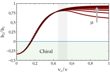
Figure 1: (color online) Variation of the coefficient ratio $b_{2}/b_{1}$ as a function of the anisotropy of the system parametrized by $v_{z}/v$ and the chemical potential $\mu$, keeping the parameter $\alpha_{z}$ fixed. For sufficiently small $v_{z}/v$ the coefficient $b_{2}$ becomes negative ($b_{1}>0$) and the chiral phase becomes possible.

The Hamiltonian Eq. (1) is linear in momentum and characteristic surface states of the TI arise when ${\rm sign}(mv_{z})<0$ for states confined in $z>0$ Hsieh and Fu (2012). Nevertheless, quadratic corrections in the mass term can be also considered and appear in more refined band structure calculationsZhang et al. (2009),

$$m({\bf k})=m-\alpha k^{2}-\alpha_{z}k_{z}^{2},$$ (10)

where $k^{2}=k_{x}^{2}+k_{y}^{2}$. For $m,\alpha,\alpha_{z}>0$ the mass term changes sign on a particular surface in momentum space. This property yields a non-trivial topology of the insulator. For simplicity we neglect a spin- and orbital-independent term that adds to the Hamiltonian as a diagonal ${\bf k}$-dependent contribution and does not change the topological properties of the system, a part from breaking the particle-hole symmetry of the Dirac Hamiltonian describing the topological insulator.

The momentum dependence of the mass term introduces a second scales $\alpha_{z}$ along the $k_{z}$ direction that, together with the velocity $v_{z}$, makes the Fermi surface intrinsically anisotropic. If $\alpha_{z}$ is neglected, the unique scale $v_{z}$ can be reabsorbed in a redefinition of the momentum and it eventually factorizes in the expression of $b_{1}$ and $b_{2}$, in a way that their value become fixed and positive. It is then reasonable to study the parameter $b_{2}$ as we increase the anisotropy of the Fermi surface by considering finite $\alpha_{z}$.

The values of $v_{z}$ and $\alpha_{z}$ can be controlled by chemical doping, in that dopants intercalate between the QLs and modify the interlayer distance $a_{z}$ and hopping $t_{z}$. The latter can be assumed to be exponentially dependent on $a_{z}$ itself, $t_{z}=t_{z}^{0}\exp(-a_{z}/R)$, with $R$ a microscopic length scale characteristic of the $p_{z}$ orbital of Se, and $t_{z}^{0}$ the amplitude of the hopping integral. It then follows that an increase in the doping is expected to lower both $v_{z}$ and $\alpha_{z}$.

In Fig. 1 we plot the dependence of $b_{2}/b_{1}$ as a function of $v_{z}/v$, keeping $\alpha_{z}$ constant and taking for reference the parameters of the well known model of Ref. [Zhang et al., 2009], $m=0.28~{}$eV, $\alpha=56.6~{}$eV Å², $\alpha_{z}=10.0~{}$eV Å², and $v=4.1~{}$eV Å. The coefficient $\alpha_{z}$ drops from the ratio. The shadowed regions indicate the region around $v_{z}=2.2~{}$eV Å, that is realized in the undoped material. We clearly see that by decreasing $v_{z}/v$ we can obtain negative $b_{2}$ values. The strong topological character of the material allows a wide range of variation of $v_{z}$ through doping, without changing the topological nature of the system, so that a chiral phase can be obtained by properly choosing the dopants and their amount.

V Chiral phase in thin slabs

In the 2D limit the Fermi surface is a line at $k_{z}=0$, the coefficient $b_{2}$ Eq. (9) is explicitly negative, and the chiral phase is stable. The case $v_{z}\to 0$ and $\alpha_{z}\to 0$ is clearly realized when the system approaches the limit of quasi decoupled layers or the quasi 2D limit, characterized by an open Fermi surfaceLahoud et al. (2013). We now study the stability of the nematic versus the chiral phase for reduced thickness of the sample by varying the number of unit cell layers.

We consider a simplified tight-binding model along the lines of Ref. [Hsieh and Fu, 2012]. We approximate the QL structure as a bilayer system (BL) composed by its top most (T) and bottom most (B) Se layers, described by triangular lattices on top of each other. The entire structure is described by the tight-binding Hamiltonian

$$H_{\rm TI}=H_{0}+H_{\rm R}+H_{z}.$$ (11)

The first term $H_{0}$ describes spin-independent hopping within the same layer and nearest neighbour tunnelling between the two layers

$$H_{0} = t_{0}\sum_{<i,j>,\sigma s}c^{\dagger}_{i,\sigma,s}c_{j,\sigma,s}+t_{1}\sum_{i}c^{\dagger}_{i,T,s}c_{i,B,s}+{\rm H.c.}$$ (12)

$$+ t_{2}\sum_{<i,j>,s}(c^{\dagger}_{i,T,s}c_{j,B,s}+c^{\dagger}_{i,B,s}c_{j,T,s}),$$

with $\sigma=T,B$ labeling the two layers. Atoms in the two layers experience local opposite electric fields along the $\pm\hat{z}$ direction, that give rise to Rashba SOI of opposite sign on the two layer in the form

$$H_{R}=i\lambda\sum_{<ij>\sigma,ss^{\prime}}p_{\sigma}c^{\dagger}_{i,\sigma,s}c_{j,\sigma,s^{\prime}}{\bf s}_{ss^{\prime}}\cdot\hat{z}\times{\bf a}_{ij},$$ (13)

with $p_{T,B}=\pm 1$ and ${\bf a}_{ij}$ a unit vector connecting site $i$ and site $j$. Finally, along the $z$-direction the structure is repeated as a series of tightly bound BL planes weakly coupled by van der Waals forces. Within the effective bilayer model the dynamics along the vertical direction can be described by an interlayer hopping term

$$H_{z}=t_{z}\sum_{j}c^{\dagger}_{j,T,s}c_{j-1,B,s}+{\rm H.c.},$$ (14)

with $t_{z}$ intercell hopping amplitude.

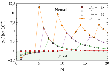
Figure 2: (color online) Variation of the coefficient $b_{2}$ as a function of the number of layers $N$ for different chemical potential. The parameter used in the tight-binding model are $t_{0}=0$, $t_{1}=-4.1~{}{\rm eV}$, $t_{2}=0.75~{}{\rm eV}$, $t_{z}=-0.6~{}{\rm eV}$, $\lambda=0.5~{}{\rm eV}$, $a=5.0~{}{\rm\AA}$, and $a_{z}=9.1~{}{\rm\AA}$.

The Hamiltonian $H_{\rm TI}$ describes a 3D TI, whose small momentum expansion well approximates the Hamiltonian Eq. (1) with in-plane velocity $v=3\lambda a$, out-of-plane velocity $v_{z}=t_{z}a_{z}$, and a mass term that depends on the momentum, $m({\bf k})=6t_{2}+t_{1}+t_{z}-3t_{2}a^{2}k^{2}/2-t_{z}a_{z}^{2}/2$, from which we extract $m=6t_{2}+t_{1}+t_{z}$, $\alpha=3t_{2}a^{2}/2$, and $\alpha_{z}=t_{z}a_{z}^{2}/2$ appearing in Eq. (10). In order to study the stability of the chiral phase for the massive Dirac model Eq. (1) we choose values of the tight-binding parameters $t_{0}$, $t_{1}$, $t_{2}$, $\lambda$, and $t_{z}$, in a way that the band structure is well described by a Dirac equation at small momentum. With the choice specified in Fig. 2 we obtain a mass $m=-0.2~{}{\rm eV}$ and velocities $v=7.5~{}{\rm eV}$Å, $v_{z}=-5.46~{}{\rm eV}$Å. These values are on order of those provided in Ref. [Zhang et al., 2009] and the resulting model well describes the complicate band structure of Bi₂Se₃ at low energy.

The coefficient $b_{2}$ is calculated with the Fourier transformed Hamiltonian $H_{\rm TI}({\bf k}_{\parallel},n_{z})=H_{\rm TI}({\bf k}_{\parallel},\pi n_{z}/Na_{z})$, where $N$ is the number of layers, and by collecting the relevant terms in the fourth order expansion projected onto the conduction band

$$F_{4}=\frac{\kappa}{N_{F}}\sum_{n_{z},{\bf k}}\delta(\xi_{{\bf k},n_{z}}){\rm Tr}[\left({\cal P}_{{\bf k},n_{z}}\Delta^{\dagger}{\cal P}_{{\bf k},n_{z}}\Delta\right)^{2}],$$ (15)

where ${\cal P}_{{\bf k},n_{z}}=\sum_{i=1,2}|\psi_{{\bf k},i}\rangle\langle\psi_{{\bf k},i}|$ is the projection operator of the conduction band subspace and $\Delta=-\psi_{x}\sigma_{y}s_{y}+\psi_{y}\sigma_{y}s_{x}$. We keep the tight-binding parameters fixed and only vary the number of layers $N$. In Fig. 2 we clearly see that the chiral phase is stable for sufficiently thin slabs of material. In particular, we see that the coefficient $b_{2}$ experiences quantum oscillations due to the coupling between the 2D layers. As a function of the chemical potential, small negative values of $b_{2}$ are obtained already for thick slabs and low doping, whereas larger negative $b_{2}$ values require higher doping and thinner slabs.

The coefficient $b_{2}$ follows the dispersion along the $z$ direction. By reducing the number of layers the energy of the subbands grows and $b_{2}$ grows accordingly. As the energy of a given subband grows above the Fermi level the coefficient $b_{2}$ suddenly drops to the successive subband until a single band remains populated below the Fermi level. At that point $b_{2}$ becomes negative, as it cannot grow any longer. This explains why for low doping a structure composed by several unit cell develops the chiral phase, whereas for high doping one has to go down to the single layer case to encounter only one band below the Fermi level. The results of Fig. 2 are quite robust to variations of the tight-binding parameters characterizing the Hamiltonian, as long as the low energy model is well captured by a massive Dirac Hamiltonian. The threshold $N$ at which the transition to the chiral state takes place depends on the actual values of the tight-binding parameters. The quantum oscillations follow the band structure profile and they appear as long as the systems displays quantization of the subbands.

VI Chiral Majorana Modes

The results presented in the previous sections show that a feasible way of obtaining a chiral phase is through exfoliation and that the extreme case of a single layer is the best candidate for chiral superconductivity. The chiral solution is given by $\boldsymbol{\psi}=\psi_{0}(1,i)$ so that the resulting gap on the Fermi surface reads

$$\Delta\propto\psi_{0}(k_{y}-ik_{x})\tilde{s}_{z},$$ (16)

where $\tilde{s}_{z}$ is the third Pauli matrix in the Kramers basis at momentum ${\bf k}$. Starting from the $k\cdot p$ Hamiltonian Eq. (1) at $k_{z}=0$ we can write the Kramer basis by employing the Manifestly Covariant Bloch Basis (MCBB) introduced in Refs. [Fu, 2015; Venderbos et al., 2016a], where the band eigenstates are chosen to be fully spin polarized along the $z$ direction at the origin of point group symmetry operations.

$$|\psi_{{\bf k},1}\rangle=\left(\begin{array}[]{c}\sqrt{\epsilon_{k}+m}\\ \sqrt{\epsilon_{k}+m}\\ ik_{x}-k_{y}\\ -ik_{x}+k_{y}\end{array}\right),|\psi_{{\bf k},2}\rangle=\left(\begin{array}[]{c}-ik_{x}-k_{y}\\ ik_{x}+k_{y}\\ \sqrt{\epsilon_{k}+m}\\ \sqrt{\epsilon_{k}+m}\\ \end{array}\right),$$ (17)

in the basis $(c_{{\bf k},T,\uparrow},c_{{\bf k},B,\uparrow},c_{{\bf k},T,\downarrow},c_{{\bf k},B,\downarrow})^{T}$, up to a normalization factor $1/(2\sqrt{\epsilon_{k}^{2}+m\epsilon_{k}})$. The action of time-reversal ${\cal T}=is_{y}K$, parity ${\cal P}=\sigma_{x}$, and mirror about $x$, $M_{x}=is_{x}$, are easily computed, resulting in the following transformation properties, ${\cal T}|\psi_{{\bf k},1}\rangle=-|\psi_{-{\bf k},2}\rangle$, ${\cal T}|\psi_{{\bf k},2}\rangle=|\psi_{-{\bf k},1}\rangle$, ${\cal P}|\psi_{{\bf k},i}\rangle=|\psi_{-{\bf k},i}\rangle$, and $M_{x}|\psi_{{\bf k},1}\rangle=i|\psi_{M_{x}{\bf k},2}\rangle$, $M_{x}|\psi_{{\bf k},2}\rangle=i|\psi_{M_{x}{\bf k},1}\rangle$. It is then clear that $|\psi_{{\bf k},1}\rangle$ and $|\psi_{{\bf k},2}\rangle$ form a Kramers doublet and represent a preferential basis that transform like a spin-1/2 object Fu (2015). It is easily seen that the gap matrix $\Delta=\Delta_{0}(-\sigma_{y}s_{y}+i\sigma_{y}s_{x})$ results in Eq. (16) when projected on the basis spanned by $|\psi_{{\bf k},1}\rangle$ and $|\psi_{{\bf k},2}\rangle$. At this point, the description in terms of the four band original massive Dirac Hamiltonian can be substituted by a simpler description of the conduction band in the MCBBFu (2015).

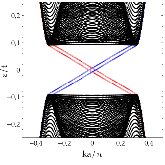
Figure 3: Bands structure of a TI single layer with chiral superconductivity on a ribbon geometry. The parameters used are $t_{0}=-0.1$, $t_{1}=-5t_{2}$, $t_{2}=1.0$, $\lambda=0.5$, $\Delta=0.1$, and $\mu=0.2$. Two Majorana edge states co-propagate on each side of the ribbon (blue on one side, red on the other side).

The BdG Hamiltonian Eq. (2) with the gap Eq. (16) projected onto the conduction band reads

$$H_{\rm BdG}=\left(\begin{array}[]{cc}\xi_{\bf k}&\Delta(k_{x}-ik_{y})\tilde{s}_{z}\\ \Delta(k_{x}+ik_{y})\tilde{s}_{z}&-\xi_{\bf k}\end{array}\right).$$ (18)

The system breaks TRI and belongs to class D topological superconductors in 2D. A finite Chern number $C_{\rm ch}=\pm 2$ is easily calculates from Eq. (18), with the sign $\pm$ depending of whether the $(1,i)$ or $(1,-i)$ solution is realized. Correspondingly two copropagating chiral Majorana modes are expected to localize at the edge of the system. This can be seen directly from inspection of Eq. (18). We see that both the spin up and spin down components are affected by a chiral $p_{x}+ip_{y}$ pairing, with gap of opposite sign for the two spin projections, due to the triplet nature of the pairing. Spinless chiral superconductivity in 2D opens a topologically non-trivial gap on the Fermi surface that gives rise to a single chiral Majorana mode at the boundary of the system, flowing with a velocity $v_{M}=\mp|\Delta|/k_{F}$, for the $p_{x}\pm ip_{y}$ cases, respectively. We then expect two chiral Majorana modes, each for spin component, that copropagate at the boundary of the system with $v_{M}=-|\Delta|/k_{F}$, with $\Delta$ the mean-field value of the order parameter $\psi_{0}$ in Eq. (16).

In order to check the predictions of the low energy effective model Eq. (18) we calculate the bands of the tight-binding model on a ribbon geometry. The mean-field Hamiltonian is $H_{\rm MF}=H+H_{\rm sc}$, with $H_{\rm sc}$ the Hamiltonian term describing superconductivity at mean field level in the chiral phase

$$H_{\rm sc}=\sum_{i;\sigma s,\sigma^{\prime}s^{\prime}}c^{\dagger}_{i,\sigma s}c^{{\dagger}}_{i,\sigma^{\prime}s^{\prime}}\hat{\Delta}_{\sigma s;\sigma^{\prime}s^{\prime}}+{\rm H.c.},$$ (19)

with $\hat{\Delta}=\Delta\sigma_{y}(s_{x}+is_{y})is_{y}$. The band structure on a ribbon geometry is shown in Fig. 3, where clear co-propagating chiral Majorana modes appear, blue on one side and red on the other side of the ribbon.

VII Conclusion

In this work we studied the stability of the chiral phase versus the nematic phase in Bi₂Se₃ as a function of the anisotropy of the system and the thickness of the sample. We showed that by increasing the two-dimensional character of the Fermi surface the chiral phase is expected to become stable. This can be experimentally achieved by properly choosing the doping element and their amount, that by intercalation modify the interlayer distance and enhance the two-dimensional character of the system. A second root towards the realization of a chiral phase is achieved by exfoliation. We found that by reducing the number of layers constituting a thin slab of material the chiral phase can be stabilized already in few layer thick slabs and, for the low doping case, exfoliation down to $N<10$ layer is expected to show the chiral phase. In particular, the single layer case is shown to always favour the chiral phase. The resulting states is a chiral topological superconductor that hosts two copropagating chiral Majorana modes at its boundary. Our findings promote single layer of Bi₂Se₃ as an ideal material for the manifestation of chiral superconductivity, opening the route to topological quantum computations with Majorana modes.

VIII Acknowledgments

The author acknowledges useful discussion with F. Finocchiaro, F. de Juan, and F. Guinea, and he is thankful to J. Schmalian for a key comment on the role of Rashba SOI. This work is supported by the European Union’s Seventh Framework Programme (FP7/2007-2013) through the ERC Advanced Grant NOVGRAPHENE (GA No. 290846) and the Comunidad de Madrid through the grant MAD2D-CM, S2013/MIT-3007.

References

- Sigrist and Ueda (1991) M. Sigrist and K. Ueda, Rev. Mod. Phys. 63, 239 (1991).
- Qi and Zhang (2011) X.-L. Qi and S.-C. Zhang, Rev. Mod. Phys. 83, 1057 (2011).
- Read and Green (2000) N. Read and D. Green, Phys. Rev. B 61, 10267 (2000).
- Ivanov (2001) D. A. Ivanov, Phys. Rev. Lett. 86, 268 (2001).
- Alicea (2012) J. Alicea, Reports on Progress in Physics 75, 076501 (2012).
- Beenakker (2013) C. W. J. Beenakker, Annual Review of Condensed Matter Physics 4, 113 (2013).
- Aguado (2017) R. Aguado, Riv. Nuovo Cimento 40, 523 (2017).
- Meng and Balents (2012) T. Meng and L. Balents, Phys. Rev. B 86, 054504 (2012).
- Sau and Tewari (2012) J. D. Sau and S. Tewari, Phys. Rev. B 86, 104509 (2012).
- Yang et al. (2014) S. A. Yang, H. Pan, and F. Zhang, Phys. Rev. Lett. 113, 046401 (2014).
- Biswas et al. (2013) P. K. Biswas, H. Luetkens, T. Neupert, T. Stürzer, C. Baines, G. Pascua, A. P. Schnyder, M. H. Fischer, J. Goryo, M. R. Lees, et al., Phys. Rev. B 87, 180503 (2013), URL https://link.aps.org/doi/10.1103/PhysRevB.87.180503.
- Fischer et al. (2014) M. H. Fischer, T. Neupert, C. Platt, A. P. Schnyder, W. Hanke, J. Goryo, R. Thomale, and M. Sigrist, Phys. Rev. B 89, 020509 (2014), URL https://link.aps.org/doi/10.1103/PhysRevB.89.020509.
- Nayak et al. (2008) C. Nayak, S. H. Simon, A. Stern, M. Freedman, and S. Das Sarma, Rev. Mod. Phys. 80, 1083 (2008).
- Sarma et al. (2015) S. D. Sarma, M. Freedman, and C. Nayak, Npj Quantum Information 1, 15001 (2015).
- Zhang et al. (2009) H. Zhang, C.-X. Liu, X.-L. Qi, X. Dai, Z. Fang, and S.-C. Zhang, Nature Physics 5, 438 (2009).
- Hasan and Kane (2010) M. Z. Hasan and C. L. Kane, Rev. Mod. Phys. 82, 3045 (2010).
- Hor et al. (2010) Y. S. Hor, A. J. Williams, J. G. Checkelsky, P. Roushan, J. Seo, Q. Xu, H. W. Zandbergen, A. Yazdani, N. P. Ong, and R. J. Cava, Phys. Rev. Lett. 104, 057001 (2010).
- Wray et al. (2010) L. A. Wray, S.-Y. Xu, Y. Xia, Y. S. Hor, D. Qian, A. V. Fedorov, H. Lin, A. Bansil, R. J. Cava, and M. Z. Hasan, Nature Physics 6, 855 (2010).
- Kriener et al. (2011) M. Kriener, K. Segawa, Z. Ren, S. Sasaki, and Y. Ando, Phys. Rev. Lett. 106, 127004 (2011).
- Sasaki et al. (2011) S. Sasaki, M. Kriener, K. Segawa, K. Yada, Y. Tanaka, M. Sato, and Y. Ando, Phys. Rev. Lett. 107, 217001 (2011).
- Levy et al. (2013) N. Levy, T. Zhang, J. Ha, F. Sharifi, A. A. Talin, Y. Kuk, and J. A. Stroscio, Phys. Rev. Lett. 110, 117001 (2013).
- Peng et al. (2013) H. Peng, D. De, B. Lv, F. Wei, and C.-W. Chu, Phys. Rev. B 88, 024515 (2013).
- Fu and Berg (2010) L. Fu and E. Berg, Phys. Rev. Lett. 105, 097001 (2010).
- Shruti et al. (2015) Shruti, V. K. Maurya, P. Neha, P. Srivastava, and S. Patnaik, Phys. Rev. B 92, 020506 (2015).
- Liu et al. (2015) Z. Liu, X. Yao, J. Shao, M. Zuo, L. Pi, S. Tan, C. Zhang, and Y. Zhang, Journal of the American Chemical Society 137, 10512 (2015).
- Wang et al. (2016) Z. Wang, A. A. Taskin, T. Frölich, M. Braden, and Y. Ando, Chemistry of Materials 28, 779 (2016).
- Asaba et al. (2017) T. Asaba, B. J. Lawson, C. Tinsman, L. Chen, P. Corbae, G. Li, Y. Qiu, Y. S. Hor, L. Fu, and L. Li, Phys. Rev. X 7, 011009 (2017).
- Matano et al. (2016) K. Matano, M. Kriener, K. Segawa, Y. Ando, and G.-q. Zheng, Nature Physics 12, 852 EP (2016).
- Yonezawa et al. (2016) S. Yonezawa, K. Tajiri, S. Nakata, Y. Nagai, Z. Wang, K. Segawa, Y. Ando, and Y. Maeno, Nature Physics 13, 123 EP (2016).
- Pan et al. (2016) Y. Pan, A. M. Nikitin, G. K. Araizi, Y. K. Huang, Y. Matsushita, T. Naka, and A. de Visser, Scientific Reports 6, 28632 EP (2016).
- Smylie et al. (2016) M. P. Smylie, H. Claus, U. Welp, W.-K. Kwok, Y. Qiu, Y. S. Hor, and A. Snezhko, Phys. Rev. B 94, 180510 (2016).
- Shen et al. (2017) J. Shen, W.-Y. He, N. F. Q. Yuan, Z. Huang, C.-w. Cho, S. H. Lee, Y. S. Hor, K. T. Law, and R. Lortz, npj Quantum Materials 2, 59 (2017).
- Fu (2014) L. Fu, Phys. Rev. B 90, 100509 (2014).
- Venderbos et al. (2016a) J. W. F. Venderbos, V. Kozii, and L. Fu, Phys. Rev. B 94, 180504 (2016a).
- Hashimoto et al. (2013) T. Hashimoto, K. Yada, A. Yamakage, M. Sato, and Y. Tanaka, Journal of the Physical Society of Japan 82, 044704 (2013).
- Nagai and Ota (2016) Y. Nagai and Y. Ota, Phys. Rev. B 94, 134516 (2016).
- Venderbos et al. (2016b) J. W. F. Venderbos, V. Kozii, and L. Fu, Phys. Rev. B 94, 094522 (2016b).
- Wu and Martin (2017a) F. Wu and I. Martin, Phys. Rev. B 95, 224503 (2017a).
- Zyuzin et al. (2017) A. A. Zyuzin, J. Garaud, and E. Babaev, Phys. Rev. Lett. 119, 167001 (2017).
- Chirolli et al. (2017) L. Chirolli, F. de Juan, and F. Guinea, Phys. Rev. B 95, 201110 (2017).
- Yuan et al. (2017) N. F. Q. Yuan, W.-Y. He, and K. T. Law, Phys. Rev. B 95, 201109 (2017).
- Wu and Martin (2017b) F. Wu and I. Martin, Phys. Rev. B 96, 144504 (2017b).
- Fernandes et al. (2012) R. M. Fernandes, A. V. Chubukov, J. Knolle, I. Eremin, and J. Schmalian, Phys. Rev. B 85, 024534 (2012).
- Hecker and Schmalian (2018) M. Hecker and J. Schmalian, npj Quantum Materials 3, 26 (2018).
- Zhang et al. (2010) Y. Zhang, K. He, C.-Z. Chang, C.-L. Song, L.-L. Wang, X. Chen, J.-F. Jia, Z. Fang, X. Dai, W.-Y. Shan, et al., Nature Physics 6, 712 EP (2010).
- Zhang et al. (2011) G. Zhang, H. Qin, J. Chen, X. He, L. Lu, Y. Li, and K. Wu, Advanced Functional Materials 21, 2351 (2011).
- Scheurer et al. (2017) M. S. Scheurer, D. F. Agterberg, and J. Schmalian, npj Quantum Materials 2, 9 (2017).
- Schnyder et al. (2008) A. P. Schnyder, S. Ryu, A. Furusaki, and A. W. W. Ludwig, Phys. Rev. B 78, 195125 (2008), URL https://link.aps.org/doi/10.1103/PhysRevB.78.195125.
- Chirolli et al. (2018) L. Chirolli, J. P. Baltanás, and D. Frustaglia, Phys. Rev. B 97, 155416 (2018), URL https://link.aps.org/doi/10.1103/PhysRevB.97.155416.
- Parhizgar and Black-Schaffer (2017) F. Parhizgar and A. M. Black-Schaffer, Scientific Reports 7, 9817 (2017).
- Nakosai et al. (2012) S. Nakosai, Y. Tanaka, and N. Nagaosa, Phys. Rev. Lett. 108, 147003 (2012).
- Fu (2015) L. Fu, Phys. Rev. Lett. 115, 026401 (2015).
- Hsieh and Fu (2012) T. H. Hsieh and L. Fu, Phys. Rev. Lett. 108, 107005 (2012).
- Lahoud et al. (2013) E. Lahoud, E. Maniv, M. S. Petrushevsky, M. Naamneh, A. Ribak, S. Wiedmann, L. Petaccia, Z. Salman, K. B. Chashka, Y. Dagan, et al., Phys. Rev. B 88, 195107 (2013).