Newton diagram of positivity for
${}_{1}F_{2}$ generalized hypergeometric functions

Abstract. As for the positivity of ${}_{1}F_{2}$ generalized hypergeometric functions, we present a list of necessary and sufficient conditions in terms of parameters and determine the region of positivity by certain Newton diagram.

Keywords. Bessel function, fractional integral, generalized hypergeometric function, Newton diagram, positivity.

2010 Mathematics Subject Classification: 33C20, 46E22, 62D05.

1 Introduction

In this paper we are concerned with the problem of positivity for the generalized hypergeometric functions of type

$${}_{1}F_{2}\left(a\,;b,c\,;\,-\frac{\,x^{2}}{4}\right)=\sum_{k=0}^{\infty}\frac{(a)_{k}}{k!(b)_{k}(c)_{k}}\left(-\frac{\,x^{2}}{4}\right)^{k}\qquad(x\in\mathbb{R}),$$ (1.1)

where the parameters $\,a,b,c\,$ are positive and the coefficients are written in Pochhammer’s symbols, that is, $\,(\alpha)_{k}=\Gamma(\alpha+k)/\Gamma(\alpha)\,$ for any $\,\alpha>0.$

In view of symmetry about zero, it will be assumed throughout $\,x>0.\,$ To simplify our notation, we shall denote by $\mathcal{P}_{1,2}$ the set of all triples $\,(a,b,c)\,$ for which the corresponding generalized hypergeometric functions are strictly positive on the interval $(0,\infty)$, that is,

$$\mathcal{P}_{1,2}=\left\{(a,b,c)\in\mathbb{R}_{+}^{3}:{}_{1}F_{2}\left(a\,;b,c\,;-\frac{\,x^{2}}{4}\right)>0\,\right\}\,.$$ (1.2)

Due to a variety of applications, the problem has been a historic issue. In classical analysis, it arises frequently in connection with the integrals or sums of those special functions expressible in terms of the generalized hypergeometric functions of type (1.1). While we refer to Askey [1], Fields and Ismail [6], Gasper [7] for further backgrounds and references, we state some of earlier results relevant to the present work.

• For $\,\alpha>-1,\,$ if $J_{\alpha}$ stands for the Bessel function of order $\alpha$, then

  $$\int_{0}^{x}J_{\alpha}(t)t^{-\beta}dt =\frac{x^{\alpha-\beta+1}}{2^{\alpha}(\alpha-\beta+1)\Gamma(\alpha+1)}$$

  $$\,\,\times\,{}_{1}F_{2}\left(\frac{\alpha-\beta+1}{2}\,;\alpha+1,\,\frac{\alpha-\beta+3}{2}\,;\,-\frac{\,x^{2}}{4}\right),$$ (1.3)

  where $\,\alpha-\beta+1>0\,$ and $B$ denotes Euler’s beta function. For its positivity, Cooke [4] proved the case $\,\beta=0\,,$ which is equivalent to

  $$(a,\,a+1,\,2a)\in\mathcal{P}_{1,2}\qquad(a>0),$$ (1.4)

  and Makai [10] proved the case $\,\beta=-1/2,\,\alpha>1/2,\,$ that is,

  $$\left(a,\,a+1,\,2a-\frac{1}{2}\right)\in\mathcal{P}_{1,2}\qquad(a>1).$$ (1.5)

• In connection with completely monotone functions of certain type and the positivity of Cesáro means of Jacobi series, Askey and Pollard [2] and Fields and Ismail [6] proved separately

  $$\left(a,\,2a,\,2a+\frac{1}{2}\right) \in\mathcal{P}_{1,2}\qquad(a>0),$$ (1.6)

  $$\left(a,\,\rho a,\,\rho a+\frac{1}{2}\right) \in\mathcal{P}_{1,2}\qquad(a>1,\,\rho\geq 3/2).$$ (1.7)

• Regarding the sign of Lommel’s function, Steinig [11] proved

  $$\left(1,\,b,\,\frac{7}{2}-b\right)\in\mathcal{P}_{1,2}\quad\left(3/2<b<2\right).$$ (1.8)

• By considering certain fractional integral transforms with the squares of Bessel functions as kernels, Gasper [7] established

  $$\left(a,\,a+\frac{1}{2}+\delta,\,2a\right)\in\mathcal{P}_{1,2}\qquad(a>0,\,\delta>0),$$ (1.9)

  which includes (1.4), (1.6) as a special case $\,\delta=1/2,\,a,\,$ respectively. In addition, as it will be explained below, Gasper invented a series expansion method for investigating positivity and obtained a number of positivity results for the Bessel integrals of certain type.

Our aim here is to determine the general patterns of parameters for positivity instead of special cases and provide information on the location of the first zeros when positivity breaks down. Our approach is based on Gasper’s method from a slightly different viewpoint and integral transforms with the squares of Bessel functions as its kernels.

To describe briefly our main result, we shall decompose the first quadrant into three disjoint regions $\,\mathbb{R}_{+}^{2}=P_{a}\cup N_{a}\cup O_{a}\,$ for each $\,a>0\,$ and prove that if $\,(b,c)\in P_{a}\,,$ then $\,(a,b,c)\in\mathcal{P}_{1,2}\,$ and if $\,(b,c)\in N_{a}\,,$ then the corresponding generalized hypergeometric function alternates in sign. It turns out that the positivity region $P_{a}$ coincides with certain Newton diagram and the missing region $O_{a}$ consists of two strips cut by the line of necessity.

2 Preliminaries

The generalized hypergeometric functions of type (1.1) includes a special class of Bessel functions defined by

$$\mathbb{J}_{\alpha}(x)={}_{0}F_{1}\left(\alpha+1\,;-\frac{\,x^{2}}{4}\right)=\Gamma(\alpha+1)\left(\frac{x}{2}\right)^{-\alpha}J_{\alpha}(x)$$ (2.1)

for $\,\alpha>-1,\,$ which will play fundamental roles in what follows.

As $\mathbb{J}_{\alpha}$ and $J_{\alpha}$ share positive zeros in common, it follows readily from the theory of Bessel functions (see [5], [9], [12]) that $\mathbb{J}_{\alpha}$ possesses infinitely many positive zeros all of which are simple and the zeros of $\mathbb{J}_{\alpha}$ and $\mathbb{J}_{\alpha+1}$ are interlaced. Moreover, if $j_{\alpha}$ denotes the smallest positive zero of $J_{\alpha}$, then

$$\frac{(3+2\alpha)\pi}{4} <j_{\alpha}<\frac{(7+2\alpha)\pi}{8}\quad\text{for}\quad|\alpha|<1/2,$$

$$\sqrt{\alpha(\alpha+2)\,} <j_{\alpha}<\sqrt{2(\alpha+1)(\alpha+3)\,}\quad\text{for}\quad\alpha>0.$$ (2.2)

If $2\alpha$ is an odd integer, then $\mathbb{J}_{\alpha}$ is expressible in terms of algebraic and trigonometric functions via the recurrence relation

$$\quad\mathbb{J}_{-\frac{1}{2}}(x)=\cos x\,,\quad\mathbb{J}_{\frac{1}{2}}(x)=\frac{\sin x}{x},$$

$$\mathbb{J}_{\alpha+1}(x)=\frac{\,4\alpha(\alpha+1)\,}{x^{2}}\left[\mathbb{J}_{\alpha}(x)-\mathbb{J}_{\alpha-1}(x)\right].$$ (2.3)

Another special class of functions is the squares of $\mathbb{J}_{\alpha}$ in the form

$$\mathbb{J}_{\alpha}^{2}\left(\frac{x}{2}\right)={}_{1}F_{2}\left(\alpha+\frac{1}{2}\,;\alpha+1,\,2\alpha+1\,;-\frac{\,x^{2}}{4}\right)$$ (2.4)

for $\,\alpha>-1/2,\,$ which will play decisive roles in determining positivity.

3 Necessity

It is simple to extend a known positivity result to other parameter cases on consideration of the fractional integral transform with appropriate kernel. Although it is observed by several authors ([1], [6], [7]), we make this basic but important aspect precise under a slightly weaker condition.

Lemma 3.1.

For $\,a>0,\,b>0,\,c>0,\,$ suppose that

$$\Phi(x)={}_{1}F_{2}\left(a\,;b,c\,;-\frac{\,x^{2}}{4}\right)\geq 0.$$

Then for any $\,0\leq\gamma<a,\,\delta\geq 0,\,\epsilon\geq 0,\,$ not simultaneously zero,

$$\,\left(a-\gamma,\,b+\delta,\,c+\epsilon\right)\in\mathcal{P}_{1,2}\,.\,$$

Proof.

Since the complex extension $\,z\mapsto\Phi(z),\,z\in\mathbb{C},\,$ is obviously entire, $\Phi$ has only isolated zeros on the interval $(0,\infty)$. For each $\,x>0,\,$ hence, it follows from the nonnegativity assumption that there exists a non-empty open interval $\,I_{x}\subset[0,1]\,$ such that $\,\Phi(xt)>0\,$ for all $\,t\in I_{x}.\,$

For $\,\delta>0\,$ and $\,x>0,\,$ it is plain to evaluate and deduce

$${}_{1}F_{2}\left(a\,;b+\delta,\,c\,;-\frac{\,x^{2}}{4}\right) =\frac{2}{B(b,\delta)}\int_{0}^{1}\Phi(xt)(1-t^{2})^{\delta-1}t^{2b-1}\,dt$$

$$\geq\frac{2}{B(b,\delta)}\int_{I_{x}}\Phi(xt)(1-t^{2})^{\delta-1}t^{2b-1}\,dt$$

$$>0.$$

In view of the integral representation

$${}_{1}F_{2}\left(a\,;b+\delta,\,c+\epsilon\,;-\frac{\,x^{2}}{4}\right)$$

$$\quad=\frac{2}{B(c,\epsilon)}\int_{0}^{1}{}_{1}F_{2}\left(a\,;b+\delta,c\,;-\frac{\,x^{2}t^{2}}{4}\right)\,(1-t^{2})^{\epsilon-1}t^{2c-1}\,dt$$

for $\,\epsilon>0,\,$ it follows from the same analysis or directly from the continuity and positivity of kernel that $\,(a,b+\delta,c+\epsilon)\in\mathcal{P}_{1,2}\,$ for any $\,\delta\geq 0,\,\epsilon\geq 0\,$ unless $\,\delta=\epsilon=0.\,$ In the last place, if $\,0<\gamma<a,\,\delta\geq 0,\,\epsilon\geq 0,\,$ then

$${}_{1}F_{2}\left(a-\gamma\,;b+\delta,\,c+\epsilon\,;-\frac{\,x^{2}}{4}\right)=\frac{2}{B(a-\gamma,\gamma)}$$

$$\quad\times\,\int_{0}^{1}{}_{1}F_{2}\left(a\,;b+\delta,c+\epsilon\,;-\frac{\,x^{2}t^{2}}{4}\right)\,(1-t^{2})^{\gamma-1}t^{2(a-\gamma)-1}\,dt,$$

which implies $\,(a-\gamma,b+\delta,c+\epsilon)\in\mathcal{P}_{1,2}\,$ by the same reasoning as above. ∎

With the aid of Lemma 3.1, an inspection on the asymptotic behavior leads to the following necessary condition for positivity and information on the location of the first zero on $(0,\infty)$ if violated. We recall that the smallest positive zero of the Bessel function $J_{\alpha}$ or $\mathbb{J}_{\alpha}$ is denoted by $j_{\alpha}$.

Theorem 3.1.

For $\,a>0,\,b>0,\,c>0,\,$ put

$$\Phi(x)={}_{1}F_{2}\left(a\,;b,\,c\,;-\frac{\,x^{2}}{4}\right)\qquad(x>0).$$

If $\,(a,b,c)\in\mathcal{P}_{1,2},\,$ then necessarily $\,b>a,\,c>a,\,b+c\geq 3a+\frac{1}{2}\,.$ Moreover, the following properties on the sign and zeros of $\Phi$ hold true.

• If $\,0<b\leq a\,$ or $\,0<c\leq a,\,$ then $\Phi$ alternates in sign and has at least one zero on the interval $\,\left(0,\,j_{c-1}\right]\,$ or $\,\left(0,\,j_{b-1}\right],$ respectively.

• Suppose that either $\,b\leq a+\frac{1}{2}\,,\,c\leq 2a\,$ or $\,b\leq 2a\,,\,c\leq a+\frac{1}{2}\,$ subject to the condition $\,b+c<3a+\frac{1}{2}.\,$ Then $\Phi$ alternates in sign and has at least one zero on the interval $\,\left(0,\,2j_{a-\frac{1}{2}}\right).$

Proof.

For $\,(a,b,c)\in\mathcal{P}_{1,2}\,,$ if $\,0<b\leq a,\,$ then Lemma 3.1 implies

$${}_{1}F_{2}\left(b\,;\,b,c\,;-\frac{\,x^{2}}{4}\right)=\mathbb{J}_{c-1}(x)>0,$$

which contradicts the fact that the Bessel function $\mathbb{J}_{c-1}$ has infinitely many zeros on the interval $(0,\infty)$. Thus $\,b>a\,$ and also $\,c>a\,$ by symmetry. In view of the asymptotic behavior (see e.g. Luke [9])

$$\Phi(x) =\frac{\Gamma(b)\Gamma(c)}{\Gamma(b-a)\Gamma(c-a)}\,\left(\frac{x}{2}\right)^{-2a}\left[1+O\left(x^{-2}\right)\right]$$

$$+\,\,\frac{\Gamma(b)\Gamma(c)}{\sqrt{\pi}\,\Gamma(a)}\,\left(\frac{x}{2}\right)^{-\sigma}\left[\cos\left(x-\frac{\pi\sigma}{2}\right)+O\left(x^{-1}\right)\right]$$ (3.1)

as $\,x\to\infty,\,$ where $\,\sigma=b+c-a-1/2,\,$ it is immediate to observe the condition $\,\sigma\geq 2a\,$ is necessary, that is, $\,b+c\geq 3a+1/2\,.$

To prove part (i), assume first $\,b=a.\,$ Then $\,\Phi(x)=\mathbb{J}_{c-1}(x)\,$ and the assertion is trivial. We next assume $\,0<b<a\,$ and represent

$$\mathbb{J}_{c-1}(x)=\frac{2x^{2-2a}}{B(b,a-b)}\int_{0}^{x}\Phi(s)(x^{2}-s^{2})^{a-b-1}s^{2b-1}ds$$

for each $\,x>0.$ Evaluating at the first positive zero of $\mathbb{J}_{c-1}$, we have

$$0=\int_{0}^{j_{c-1}}\Phi(s)\left(j_{c-1}^{2}-s^{2}\right)^{a-b-1}s^{2b-1}ds,$$

which, together with $\,\Phi(0)=1,\,$ implies that $\Phi$ must possess at least one zero on $\,\bigl{(}0,\,j_{c-1}\bigr{)}\,$ and alternate in sign. The case $\,0<c\leq a\,$ is similar.

To prove part (ii), assume first $\,b=a+\frac{1}{2}\,,\,0<c<2a.$ Since

$$\mathbb{J}_{a-\frac{1}{2}}^{2}\left(\frac{x}{2}\right) ={}_{1}F_{2}\left(a\,;a+\frac{1}{2}\,,\,2a\,;-\frac{\,x^{2}}{4}\right)$$

$$=\frac{2x^{2-4a}}{B(c,2a-c)}\int_{0}^{x}\Phi(s)(x^{2}-s^{2})^{2a-c-1}s^{2c-1}ds$$

for each $\,x>0,$ we may conclude by the same reasoning as above that $\Phi$ alternates in sign and has at least one zero on the interval $\,\left(0,\,2j_{a-\frac{1}{2}}\right).$ We next assume $\,0<b<a+\frac{1}{2}\,,\,0<c<2a.$ In this case, we set

$$\Psi(x)={}_{1}F_{2}\left(a\,;a+\frac{1}{2}\,,\,c\,;-\frac{\,x^{2}}{4}\right)$$

and deduce the following integral representations

$$\Psi(x) =\frac{2x^{1-2a}}{B\left(b,a+\frac{1}{2}-b\right)}\int_{0}^{x}\Phi(s)(x^{2}-s^{2})^{a-b-\frac{1}{2}}s^{2b-1}ds,$$

$$\mathbb{J}_{a-\frac{1}{2}}^{2}\left(\frac{x}{2}\right) =\frac{2x^{2-4a}}{B\left(c,2a-c\right)}\int_{0}^{x}\Psi(s)(x^{2}-s^{2})^{2a-c-1}s^{2c-1}ds$$

for each $\,x>0.$ Evaluating at $\,x=2j_{a-\frac{1}{2}}\,,$ the second identity implies that $\Psi$ must have a zero on $\,\left(0,\,2j_{a-\frac{1}{2}}\right),$ say, at $\,x_{0}.$ Evaluating in turn at $\,x=x_{0},\,$ the first identity implies that $\Phi$ must alternate in sign and have a zero on $(0,x_{0}).$ Thus we deduce the same conclusion as before. In view of symmetry, the proof for part (ii) is now complete. ∎

Remark 3.1.

As our proof and graphical simulations suggest, it is plausible that if $\,0<b<a,\,$ then $\Phi$ possesses infinitely many zeros and the zeros of $\Phi$ and $\mathbb{J}_{c-1}$ are interlaced but we were not able to prove or disprove.

By modifying the proof of Theorem 3.1 in an obvious way, it is not hard to deduce the following counterpart of Lemma 3.1 useful in extending a known non-positivity result to other parameter cases.

Lemma 3.2.

For $\,a>0,\,b>0,\,c>0,\,$ put

$$\Phi(x)={}_{1}F_{2}\left(a\,;b,c\,;-\frac{\,x^{2}}{4}\right).$$

If $\Phi$ alternates in sign and $z_{1}$ denotes the first zero on $(0,\infty)$, then for any $\,\gamma\geq 0,\,0\leq\delta<b,\,0\leq\epsilon<c,\,$ the function $\Psi$ defined by

$$\Psi(x)={}_{1}F_{2}\left(a+\gamma\,;b-\delta,\,c-\epsilon\,;-\frac{\,x^{2}}{4}\right)$$

also alternates in sign and possesses at least one zero on $(0,z_{1}].$

4 Integral transform method

If we take the squares of Bessel functions in the form

$${}_{1}F_{2}\left(a\,;a+\frac{1}{2}\,,\,2a\,;-\frac{\,x^{2}}{4}\right)=\mathbb{J}_{a-\frac{1}{2}}^{2}\left(\frac{x}{2}\right)\geq 0,$$

then it is straightforward to deduce by Lemma 3.1 and Theorem 3.1 the following positivity results for which we shall omit proofs.

Theorem 4.1.

For $\,a>0,\,$ if $\,b\geq a+\frac{1}{2}\,,\,c\geq 2a\,$ or $\,b\geq 2a\,,\,c\geq a+\frac{1}{2}\,$ subject to the condition $\,b+c>3a+\frac{1}{2}\,,$ then $\,(a,b,c)\in\mathcal{P}_{1,2}\,$ and the following additional properties hold true.

• $\,(a,b,2a)\in\mathcal{P}_{1,2}\,$ if and only if $\,b>a+\frac{1}{2}\,$ and

  $${}_{1}F_{2}\left(a\,;a+\frac{1}{2}+\delta,\,2a\,;-\frac{\,x^{2}}{4}\right)$$

  $$\quad=\frac{2}{B\left(\delta,a+\frac{1}{2}\right)}\int_{0}^{1}\mathbb{J}_{a-\frac{1}{2}}^{2}\left(\frac{xt}{2}\right)(1-t^{2})^{\delta-1}t^{2a}dt>0\qquad(\delta>0).$$

• $\,\left(a,a+\frac{1}{2},c\right)\in\mathcal{P}_{1,2}\,$ if and only if $\,c>2a\,$ and

  $${}_{1}F_{2}\left(a\,;a+\frac{1}{2}\,,\,2a+\epsilon\,;-\frac{\,x^{2}}{4}\right)$$

  $$\quad=\frac{2}{B\left(\epsilon,2a\right)}\int_{0}^{1}\mathbb{J}_{a-\frac{1}{2}}^{2}\left(\frac{xt}{2}\right)(1-t^{2})^{\epsilon-1}t^{4a-1}dt>0\qquad(\epsilon>0).$$

As noted earlier, the sufficiency of (i) owes to Gasper [7]. Noteworthy are the following special cases.

(A1)

The choice $\,\epsilon=1-a\,$ in (ii) yields

$${}_{1}F_{2}\left(a\,;a+\frac{1}{2}\,,\,a+1\,;-\frac{\,x^{2}}{4}\right)$$

$$\qquad=\frac{2}{B\left(1-a,2a\right)}\int_{0}^{1}\mathbb{J}_{a-\frac{1}{2}}^{2}\left(\frac{xt}{2}\right)\frac{t^{4a-1}\,dt}{(1-t^{2})^{a}}>0\quad(0<a<1).$$ (4.1)

As an application, we give an affirmative answer for an open question of Fields and Ismail [6] regarding positivity of the generalized hypergeometric function of the form (1.7) for $\,3/2<\rho<2\,$ at some value $\,0<a<1.$

Corollary 4.1.

For $\,\frac{3}{2}<\rho<2,\,$ there exists $\,\frac{1}{2}<a<1\,$ such that

$${}_{1}F_{2}\left(a\,;\rho a,\,\rho a+\frac{1}{2}\,;-\frac{\,x^{2}}{4}\right)>0.$$

Proof.

Take $\,a=1/2(\rho-1)\,$ in (4). ∎

(A2)

The choice $\,a=1\,$ in (ii) yields

$${}_{1}F_{2}\left(1\,;\frac{3}{2}\,,\,2+\epsilon\,;-\frac{\,x^{2}}{4}\right)$$

$$\qquad=\frac{8\epsilon(\epsilon+1)}{x^{2}}\int_{0}^{1}\sin^{2}\left(\frac{xt}{2}\right)(1-t^{2})^{\epsilon-1}t\,dt>0\qquad(\epsilon>0).$$ (4.2)

A rearrangement of parameters in the form $\,\epsilon+1/2=\delta\,$ leads to a simple proof of positivity for Struve’s function (cf. Watson [12]).

Corollary 4.2.

For $\,\delta>\frac{1}{2}\,$ and $\,x>0,$ Struve’s function is positive with

$$\mathbf{H}_{\delta}(x) =\frac{2\left(x/2\right)^{\delta+1}}{\sqrt{\pi}\,\Gamma(\delta+3/2)}\,{}_{1}F_{2}\left(1\,;\frac{3}{2},\,\frac{3}{2}+\delta\,;\,-\frac{\,x^{2}}{4}\right)$$

$$=\frac{(2\delta-1)(2\delta+1)\left(x/2\right)^{\delta-1}}{\sqrt{\pi}\,\Gamma(\delta+3/2)}\int_{0}^{1}\sin^{2}\left(\frac{xt}{2}\right)(1-t^{2})^{\delta-\frac{3}{2}}\,t\,dt>0.$$

5 Gasper’s series method

In [7] Gasper discovered a series expansion formula for an arbitrary ${}_{p}F_{p+1}$ generalized hypergeometric function in terms of squares of Bessel functions, which sets up a remarkably effective method for inspecting positivity when the signs of coefficients are deterministic.

In a slightly different form, Gasper’s formula asserts in effect

$${}_{1}F_{2}\left(a\,;b,\,c\,;\,-\frac{\,x^{2}}{4}\right)=\mathbb{J}_{\nu}^{2}\left(\frac{x}{2}\right)+R_{\nu}(x),$$

$$\quad R_{\nu}(x)=\sum_{n=1}^{\infty}\frac{S(n,\nu)}{n!}\frac{2n+2\nu}{n+2\nu}\frac{(2\nu+1)_{n}}{(\nu+1)_{n}^{2}}\left(\frac{x}{4}\right)^{2n}\mathbb{J}^{2}_{n+\nu}\left(\frac{x}{2}\right),$$ (5.1)

where $\nu$ is any real such that $2\nu$ is not a negative integer and

$$S(n,\nu)={}_{4}F_{3}\left(\begin{array}[]{c}-n,\,\,n+2\nu,\,\,\nu+1,\,\,a\\ \nu+\frac{1}{2},\,\,b,\,\,c\end{array}\biggl{|}1\right).$$ (5.2)

In view of the interlacing property on the zeros of Bessel functions, Gasper’s formula (5) can be interpreted as follows.

• If the coefficients of $R_{\nu}$ are all positive, then $\,(a,b,c)\in\mathcal{P}_{1,2}\,$ with

  $${}_{1}F_{2}\left(a\,;b,\,c\,;\,-\frac{\,x^{2}}{4}\right)>\mathbb{J}_{\nu}^{2}\left(\frac{x}{2}\right).$$ (5.3)

• If the coefficients of $R_{\nu}$ are all negative, then

  $${}_{1}F_{2}\left(a\,;b,\,c\,;\,-\frac{\,x^{2}}{4}\right)<\mathbb{J}_{\nu}^{2}\left(\frac{x}{2}\right)$$ (5.4)

  so that it possesses at least one zero on the interval $\left(0,\,2j_{\nu}\right).$

To implement Gasper’s series method, we shall reduce $S(n,\nu)$ to a ${}_{3}F_{2}$ terminating series for which two types of summation formulas are available. For each integer $n$, Saalschüz’s formula asserts

$${}_{3}F_{2}\left(\begin{array}[]{c}-n,\,n+\alpha,\,\beta\\ \gamma,\,1+\alpha+\beta-\gamma\end{array}\biggl{|}1\right) =\frac{(\alpha+1-\gamma)_{n}(\gamma-\beta)_{n}}{(\gamma)_{n}(1+\alpha+\beta-\gamma)_{n}}$$ (5.7)

and Watson’s formula takes the form

$${}_{3}F_{2}\left(\begin{array}[]{c}-n,\,n+2\alpha,\,\beta\\ \alpha+1/2\,,\,2\beta\end{array}\biggl{|}1\right)=\frac{(1/2)_{k}(\alpha+1/2-\beta)_{k}}{(\alpha+1/2)_{k}(\beta+1/2)_{k}}$$ (5.10)

if $\,n=2k,\,k=1,2,\cdots,\,$ and zero otherwise. Both formulas are valid if the denominators are not equal to zero (see Bailey [3] and Luke [9]).

On account of symmetry in $\,b,c,\,$ there are only three possible ways of reduction. In the first place, if we take $\,\nu=a-1/2\,$ and $\,b+c=3a+1/2,\,$ the boundary plane of the necessity region for positivity, then our evaluation of $S(n,\nu)$ by Saalschüz’s formula (5.7) gives the series development

$${}_{1}F_{2}\left(a\,;b,\,3a+\frac{1}{2}-b\,;-\frac{\,x^{2}}{4}\right)$$

$$\qquad\quad=\mathbb{J}_{a-\frac{1}{2}}^{2}\left(\frac{x}{2}\right)+\sum_{n=1}^{\infty}\frac{2n+2a-1}{n+2a-1}\frac{(2a)_{n}}{n!\,(a+1/2)_{n}^{2}}$$

$$\qquad\qquad\quad\times\,\,\frac{(2a-b)_{n}\left(b-a-1/2\right)_{n}}{(b)_{n}\left(3a+1/2-b\right)_{n}}\left(\frac{x}{4}\right)^{2n}\mathbb{J}^{2}_{n+a-\frac{1}{2}}\left(\frac{x}{2}\right).$$ (5.11)

Theorem 5.1.

For $\,a>0,\,b>0,\,$ we have

$$\left(a,\,b,\,3a+\frac{1}{2}-b\right)\in\mathcal{P}_{1,2}$$ (5.12)

if and only if $\,a\neq 1/2\,$ and $b$ lies strictly between $\,a+1/2\,$ and $2a$. Moreover, the following inequality holds true in such a case:

$${}_{1}F_{2}\left(a\,;b,\,3a+\frac{1}{2}-b\,;-\frac{\,x^{2}}{4}\right)>\mathbb{J}_{a-\frac{1}{2}}^{2}\left(\frac{x}{2}\right)$$ (5.13)

Proof.

In view of the necessity for positivity, it suffices to deal with the case $\,a<b<2a+1/2\,.$ An inspection on Gasper’s sum (5) reveals the coefficients are all positive if $\,2a<b<a+1/2\,$ for $\,0<a<1/2\,$ or $\,a+1/2<b<2a\,$ for $\,a>1/2\,$ and all negative otherwise. Hence the assertion follows and the inequality (5.13) is a simple consequence of our interpretation (5.3).

In the case $\,a=1/2,\,1/2<b<3/2,\,$ (5) reduces to

$${}_{1}F_{2}\left(\frac{1}{2}\,;b,\,2-b\,;-\frac{\,x^{2}}{4}\right)$$

$$\qquad=\mathbb{J}_{0}^{2}\left(\frac{x}{2}\right)+2\sum_{n=1}^{\infty}\frac{(1-b)_{n}\left(b-1\right)_{n}}{(n!)^{2}\,(b)_{n}\left(2-b\right)_{n}}\left(\frac{x}{4}\right)^{2n}\mathbb{J}^{2}_{n}\left(\frac{x}{2}\right).$$

If $\,b\neq 1,\,$ then the coefficients of the series on the right are easily seen to be negative and hence the function on the left must possess at least one zero on the interval $\left(0,\,2j_{0}\right).$ If $\,b=1,\,$ then the series vanishes and

$${}_{1}F_{2}\left(\frac{1}{2}\,;1,\,1\,;-\frac{\,x^{2}}{4}\right)=\mathbb{J}_{0}^{2}\left(\frac{x}{2}\right),$$

which possesses infinitely many zeros. ∎

Remark 5.1.

In the case when positivity breaks down, it is not hard to figure out the cases of $\,a,b\,$ in which the opposite inequality

$${}_{1}F_{2}\left(a\,;b,\,3a+\frac{1}{2}-b\,;-\frac{\,x^{2}}{4}\right)<\mathbb{J}_{a-\frac{1}{2}}^{2}\left(\frac{x}{2}\right)$$ (5.14)

holds true, e.g., the case $\,a<b<2a,\,0<a<\frac{1}{2}\,$ or $\,a<b<a+\frac{1}{2},\,a>\frac{1}{2}\,,$ which implies the function on the right alternates in sign and possesses at least one zero on the interval $\,\left(0,\,2j_{a-\frac{1}{2}}\right)$.

As an illustration, we take $\,a=1/8\,$ and $\,b=3/8\,$ to see

$$\mathbb{J}_{-\frac{3}{8}}^{2}\left(\frac{x}{2}\right)<{}_{1}F_{2}\left(\frac{1}{8}\,;\frac{3}{8},\,\frac{1}{2}\,;-\frac{\,x^{2}}{4}\right)=\Phi_{1}(x).$$

For the opposite monotonicity, we take $\,b=3/16\,$ to see

$$\mathbb{J}_{-\frac{3}{8}}^{2}\left(\frac{x}{2}\right)>{}_{1}F_{2}\left(\frac{1}{8}\,;\frac{3}{16},\,\frac{11}{16}\,;-\frac{\,x^{2}}{4}\right)=\Phi_{2}(x).$$

In Figure 5.1, each curve from the top represents $\,\Phi_{1}(x),\,\mathbb{J}_{-\frac{3}{8}}^{2}\left(\frac{x}{2}\right),\,\Phi_{2}(x).\,$

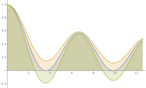
Figure 5.1: Monotonicity of generalized hypergeometric functions

(B1)

If we consider the dilation $\,b=\rho a,\,1<\rho<2,\,$ then

$$\left(a,\,\rho a,\,(3-\rho)a+\frac{1}{2}\right)\in\mathcal{P}_{1,2}\quad\text{if and only if}\quad a>\frac{1}{2(\rho-1)}\,.$$ (5.15)

The special case $\,\rho=3/2\,$ gives (1.7), the result of Fields and Ismail, where the restriction $\,a>1\,$ is sufficient and necessary.

(B2)

A necessary and sufficient condition for

$$\left(a,\,a+\delta,\,2a+\frac{1}{2}-\delta\right)\in\mathcal{P}_{1,2}$$

is that either $\,0<\delta<\frac{1}{2},\,0<a<\delta\,$ or $\,\delta>\frac{1}{2},\,a>\delta.$ The special case $\,\delta=1\,$ gives Makai’s result (1.5) in a sharp form.

(B3)

A number of interesting positivity results are obtainable by either fixing $a$ and varying $b$ or fixing $b$ and varying $a$. For instance, we have

$$\left(1,\,b,\,\frac{7}{2}-b\right) \in\mathcal{P}_{1,2}\quad\text{if and only if}\quad\frac{3}{2}<b<2,$$

$$\left(a,\,\frac{3}{4},\,3a-\frac{1}{4}\right) \in\mathcal{P}_{1,2}\quad\text{if and only if}\quad\frac{1}{4}<a<\frac{3}{8}$$

for which the former corresponds to Steinig’s result [11] on the positivity of Lommel’s function in a sharp form.

In the second place, if $\,\nu=b-1,\,c=a+b-1/2\,,\,$ then our reduction and evaluation of $S(n,\nu)$ by Saalschüz’s formula (5.7) yield

$${}_{1}F_{2}\left(a\,;b,\,a+b-\frac{1}{2}\,;-\frac{\,x^{2}}{4}\right)$$

$$\qquad\quad=\mathbb{J}_{b-1}^{2}\left(\frac{x}{2}\right)+\sum_{n=1}^{\infty}\frac{2n+2b-2}{n+2b-2}\frac{(2b-1)_{n}}{n!\,(b)_{n}^{2}}$$

$$\qquad\qquad\qquad\times\,\,\frac{\left(b-a-1/2\right)_{n}}{\left(a+b-1/2\right)_{n}}\left(\frac{x}{4}\right)^{2n}\mathbb{J}^{2}_{n+b-1}\left(\frac{x}{2}\right)$$ (5.16)

and we obtain the following positivity result by analyzing the coefficients along the same lines of reasonings as before.

Theorem 5.2.

For $\,a>0,\,b>0,\,$ we have

$$\left(a,\,b,\,a+b-\frac{1}{2}\right)\in\mathcal{P}_{1,2}\quad\text{if and only if}\quad b>a+\frac{1}{2}.$$ (5.17)

Moreover, the following inequality holds true in such a case:

$${}_{1}F_{2}\left(a\,;b,\,a+b-\frac{1}{2}\,;-\frac{\,x^{2}}{4}\right)>\mathbb{J}_{b-1}^{2}\left(\frac{x}{2}\right).$$ (5.18)

(B4)

We have $\,(a,\,a+1,\,3/2)\in\mathcal{P}_{1,2}\,$ if and only if $\,0<a<1\,$ with

$${}_{1}F_{2}\left(a\,;a+1,\,\frac{3}{2}\,;-\frac{\,x^{2}}{4}\right) =\frac{\pi}{x}\,\sum_{n=0}^{\infty}(2n+1)\frac{(1-a)_{n}}{(1+a)_{n}}J^{2}_{n+\frac{1}{2}}\left(\frac{x}{2}\right)$$

$$>\left[\frac{\sin(x/2)}{x/2}\right]^{2}\,=\mathbb{J}_{\frac{1}{2}}^{2}\left(\frac{x}{2}\right).$$ (5.19)

As an application of (5), we obtain the positivity of the generalized sine integral (see Luke [9]) in the form

$$\int_{0}^{x}t^{-\delta}\sin t\,dt =\frac{x^{2-\delta}}{2-\delta}\cdot{}_{1}F_{2}\left(\frac{2-\delta}{2}\,;\frac{4-\delta}{2}\,,\,\frac{3}{2}\,;-\frac{\,x^{2}}{4}\right)$$

$$=\frac{\pi x^{1-\delta}}{2-\delta}\,\sum_{n=0}^{\infty}(2n+1)\frac{(\delta/2)_{n}}{(2-\delta/2)_{n}}J^{2}_{n+\frac{1}{2}}\left(\frac{x}{2}\right)$$

$$>\frac{x^{2-\delta}}{2-\delta}\cdot\left[\frac{\sin(x/2)}{x/2}\right]^{2}\qquad(0<\delta<2)$$ (5.20)

(see Watson [12], pp. 152, for the case $\,\delta=1\,$).

In the last place, if $\,\nu=b-1,\,c=2a,\,$ then our reduction and evaluation of $S(n,\nu)$ by Watson’s formula (5.10) read as

$${}_{1}F_{2}\left(a\,;b,\,2a\,;-\frac{\,x^{2}}{4}\right) =\mathbb{J}_{b-1}^{2}\left(\frac{x}{2}\right)+\sum_{n=1}^{\infty}\frac{2n+b-1}{n+b-1}\frac{(b)_{n}}{n!\,(b)_{2n}^{2}}$$

$$\quad\times\,\,\frac{\left(b-a-1/2\right)_{n}}{\left(a+1/2\right)_{n}}\left(\frac{x}{4}\right)^{4n}\mathbb{J}^{2}_{2n+b-1}\left(\frac{x}{2}\right),$$ (5.21)

which yields the following result.

Theorem 5.3.

For $\,a>0,\,b>0,\,$ we have

$$\left(a,\,b,\,2a\right)\in\mathcal{P}_{1,2}\quad\text{if and only if}\quad b>a+\frac{1}{2}$$ (5.22)

and the following inequality holds true in such a case:

$${}_{1}F_{2}\left(a\,;b,\,2a\,;-\frac{\,x^{2}}{4}\right)>\mathbb{J}_{b-1}^{2}\left(\frac{x}{2}\right).$$ (5.23)

We should point out that this positivity result is already obtained by the integral transform method in part (i) of Theorem 4.1. The only difference is the inequality (5.23) which gives a deeper insight on positivity.

Remark 5.2.

For $\,a<b<a+\frac{1}{2}\,,$ it is simple to deduce

$${}_{1}F_{2}\left(a\,;b,\,a+b-\frac{1}{2}\,;-\frac{\,x^{2}}{4}\right) <\mathbb{J}_{b-1}^{2}\left(\frac{x}{2}\right),$$ (5.24)

$${}_{1}F_{2}\left(a\,;b,\,2a\,;-\frac{\,x^{2}}{4}\right) <\mathbb{J}_{b-1}^{2}\left(\frac{x}{2}\right)$$ (5.25)

from Theorems 5.2 and 5.3 so that each function on the right alternates in sign and possesses at least one zero on the interval $\,\left(0,\,2j_{b-1}\right)$.

6 Newton diagram of positivity

Collecting all of our preceding results, it is straightforward to determine the regions of positivity and non-positivity in the first quadrant for each fixed $\,a>0\,$ with the aid of Lemma 3.1 and Lemma 3.2.

To state, we shall denote by $O_{a}$ the set of all points $\,(b,c)\in\mathbb{R}_{+}^{2}\,$ defined in terms of interval notation as follows:

$$O_{a} =\left(a,\,a+\frac{1}{2}\right)\times\left[3a+\frac{1}{2}-b,\,\infty\right)$$

$$\quad\cup\left(2a,\,2a+\frac{1}{2}\right)\times\left[3a+\frac{1}{2}-b,\,a+\frac{1}{2}\right)$$

$$\quad\cup\left[2a+\frac{1}{2},\,\infty\right)\times\left(a,\,a+\frac{1}{2}\right)\quad\text{if}\quad a\geq\frac{1}{2}\,,$$ (6.1)

$$O_{a} =\left(a,\,2a\right)\times\left[3a+\frac{1}{2}-b,\,\infty\right)$$

$$\quad\cup\left(a+\frac{1}{2},\,2a+\frac{1}{2}\right)\times\left[3a+\frac{1}{2}-b,\,2a\right)$$

$$\quad\cup\left[2a+\frac{1}{2},\,\infty\right)\times\left(a,\,2a\right)\quad\text{if}\quad 0<a<\frac{1}{2}\,.$$ (6.2)

As it is standard, the Newton diagram associated to a finite set of plane points $\,\bigl{\{}\left(\alpha_{i},\,\beta_{i}\right):i=1,\cdots,N\bigr{\}}\,$ refers to the convex hull containing

$$\bigcup_{i=1}^{N}\,\bigl{\{}(x,y)\in\mathbb{R}^{2}:x\geq\alpha_{i},\,\,y\geq\beta_{i}\bigr{\}}\,.$$

Theorem 6.1.

For $\,a>0,\,$ put

$$\Phi(x)={}_{1}F_{2}\left(a\,;b,c\,;-\frac{\,x^{2}}{4}\right).$$

Let $P_{a}$ be the Newton diagram associated to $\,\Lambda=\left\{\left(a+\frac{1}{2},\,2a\right),\,\left(2a,\,a+\frac{1}{2}\right)\right\},\,$ $O_{a}$ the set defined as in (6.1), (6.2) and $N_{a}$ the complement of $\,P_{a}\cup O_{a}\,$ in $\mathbb{R}_{+}^{2}$ so that the decomposition $\,\mathbb{R}_{+}^{2}=P_{a}\cup O_{a}\cup N_{a}\,$ holds.

• If $\,(b,c)\in P_{a}\,,$ then $\,\Phi\geq 0\,$ and strict positivity holds unless $(b,c)\in\Lambda.$

• If $\,(b,c)\in N_{a}\,,$ then $\Phi$ alternates in sign and possesses at least one zero on the interval $(0,\infty).$

Remark 6.1.

For $\,(b,c)\in O_{a}\,,$ we do not know if $\Phi$ is positive or alternates in sign. We include Figure 6.1 to illustrate $\,P_{a},\,O_{a},\,N_{a}\,$ in the case $\,a>\frac{1}{2}\,.$

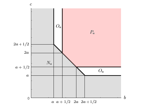
Figure 6.1: Newton diagram of positivity for $\,a>\frac{1}{2}$

As an application, we consider the problem of positivity for the Bessel integral ((i)). By Theorem 3.1, the necessity region is easily seen to be

$$C=\left\{(\alpha,\beta):\alpha>-1,\,\,\beta\geq-\frac{1}{2}\,,\,\,-\alpha-1<\beta<\alpha+1\right\}\,.$$

Applying Theorem 6.1 case by case, it is straightforward to deduce

$$\int_{0}^{x}J_{\alpha}(t)t^{-\beta}dt>0\quad\text{for}\quad(\alpha,\beta)\in A=C\setminus B,$$ (6.3)

as depicted in Figure 6.2, where $B$ denotes the parallelogram given by

$$B=\left\{(\alpha,\beta):-1<\alpha+\beta<0,\,\,-\frac{1}{2}\leq\beta<0\right\}\,.$$

As a limiting case of certain sums of Jacobi polynomials, the positivity of ((i)) has been investigated by many authors and we refer to Askey [1] for its historical backgrounds. We should remark that Askey also obtained the positivity region $A$ by using an interpolation argument for which the earlier results (1.4), (1.5) of Cooke and Makai play the roles of end-points.

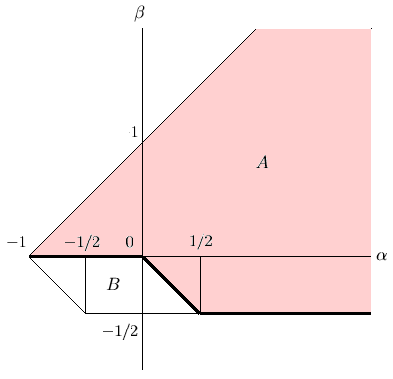
Figure 6.2: The region of positivity for the Bessel integral

7 An extension theorem

Although it is far beyond the scope of the present work, it would be worthwhile to indicate how our results could be extended in a simple way to the ${}_{p}F_{p+1}$ generalized hypergeometric functions of certain type.

Theorem 7.1.

Suppose that $\,\alpha>0,\,\beta>0,\,\gamma>0\,$ and

$${}_{1}F_{2}\left(\alpha\,;\beta,\,\gamma\,;-\frac{\,x^{2}}{4}\right)\geq 0.$$

If $\,p\geq 2\,$ and $\,0<a_{j}<b_{j}\,,\,j=1,\cdots,p-1,\,$ then

$$\Phi(x)={}_{p}F_{p+1}\left(\begin{array}[]{c}\alpha,\,a_{1},\cdots,a_{p-1}\\ \beta,\,\gamma,\,b_{1},\cdots,b_{p-1}\end{array}\biggl{|}-\frac{\,x^{2}}{4}\right)>0.$$

Proof.

By an elementary computation, it is plain to represent

$$\Phi(x) =\prod_{j=1}^{p-1}\frac{2}{B(a_{j},\,b_{j}-a_{j})}\int_{0}^{1}\cdots\int_{0}^{1}{}_{1}F_{2}\left(\alpha\,;\beta,\,\gamma\,;-\frac{\,x^{2}t_{1}^{2}\cdots t_{p-1}^{2}}{4}\right)$$

$$\qquad\qquad\qquad\times\quad\left[\prod_{j=1}^{p-1}(1-t_{j}^{2})^{b_{j}-a_{j}-1}t_{j}^{2a_{j}-1}\right]dt_{1}\cdots dt_{p-1}.$$

and the result follows by the same reasonings as we have adopted before. ∎

As an illustration, let us consider

$$\Phi_{1}(x) ={}_{2}F_{3}\left(\frac{1}{2}\,,\,1\,;\frac{3}{4}\,,\,\frac{3}{2}\,,\,2\,;-\frac{\,x^{2}}{4}\right),$$

$$\Phi_{2}(x) ={}_{2}F_{3}\left(\frac{1}{2}\,,\,1\,;\frac{5}{4}\,,\,\frac{5}{4}\,,\,3\,;-\frac{\,x^{2}}{4}\right).$$

Since $\,(1,\,3/2,\,2)\,$ corresponds to the square $\,\mathbb{J}_{\frac{1}{2}}^{2}\left(\frac{x}{2}\right),\,$ we conclude $\,\Phi_{1}>0\,$ and Theorem 6.1 gives $\,(1/2,\,5/4,\,5/4)\in\mathcal{P}_{1,2}\,$ so that $\,\Phi_{2}>0.\,$

Acknowledgements. Yong-Kum Cho is supported by National Research Foundation of Korea Grant funded by the Korean Government (# 20160925). Hera Yun is supported by the Chung-Ang University Research Scholarship Grants in 2014-2015.

Yong-Kum Cho (ykcho@cau.ac.kr) and Hera Yun (herayun06@gmail.com)

Department of Mathematics, College of Natural Science, Chung-Ang University, 84 Heukseok-Ro, Dongjak-Gu, Seoul 156-756, Korea

References

- [1] R. Askey, Problems which interest and/or annoy me, J. Comput. Appl. Math. 48, pp. 3–15 (1993)
- [2] R. Askey and H. Pollard, Some absolutely monotonic and completely monotone functions, SIAM J. Math. Anal. 5, pp. 58–63 (1974)
- [3] W. N. Bailey, Generalized Hypergeometric Series, Cambridge University Press, Cambridge (1935)
- [4] R. G. Cooke, A monotonic property of Bessel functions, J. London Math. Soc. 12, pp. 180–185 (1937)
- [5] A. Erdélyi (editor), Higher transcendental Functions (Volume II), McGraw-Hill (1953)
- [6] J. Fields and M. Ismail, On the positivity of some ’s, SIAM J. Math. Anal. 6, pp. 551–559 (1975)
- [7] G. Gasper, Positive integrals of Bessel functions, SIAM J. Math. Anal. 6, pp. 868–881 (1975)
- [8] G. Gasper, Positive sums of the classical orthogonal polynomials, SIAM J. Math. Anal. 8, pp. 423–447 (1977)
- [9] Y. L. Luke, The Special Functions and Their Approxiations, Vol. I, II, Academic Press, New York (1969)
- [10] E. Makai, On a monotonic property of certain Sturm-Liouville functions, Acta Math. Acad. Sci. Hungar. 3, pp. 165–172 (1952)
- [11] J. Steinig, The sign of Lommel’s function, Trans. Amer. Math. Soc. 163, pp. 123–129 (1972)
- [12] G. N. Watson, A Treatise on the Theory of Bessel Functions, Cambridge University Press, London (1922)