Log-concave sampling:
Metropolis-Hastings algorithms are fast

Abstract

We study the problem of sampling from a strongly log-concave density supported on $\mathbb{R}^{d}$, and prove a non-asymptotic upper bound on the mixing time of the Metropolis-adjusted Langevin algorithm (MALA). The method draws samples by simulating a Markov chain obtained from the discretization of an appropriate Langevin diffusion, combined with an accept-reject step. Relative to known guarantees for the unadjusted Langevin algorithm (ULA), our bounds show that the use of an accept-reject step in MALA leads to an exponentially improved dependence on the error-tolerance. Concretely, in order to obtain samples with TV error at most $\delta$ for a density with condition number $\kappa$, we show that MALA requires $\mathcal{O}\big{(}\kappa d\log(1/\delta)\big{)}$ steps from a warm start, as compared to the $\mathcal{O}\big{(}\kappa^{2}d/\delta^{2}\big{)}$ steps established in past work on ULA. We also demonstrate the gains of a modified version of MALA over ULA for weakly log-concave densities. Furthermore, we derive mixing time bounds for the Metropolized random walk (MRW) and obtain $\mathcal{O}(\kappa)$ mixing time slower than MALA. We provide numerical examples that support our theoretical findings, and demonstrate the benefits of Metropolis-Hastings adjustment for Langevin-type sampling algorithms.

Keywords: Log-concave sampling, Langevin algorithms, MCMC algorithms, conductance methods

1 Introduction

Drawing samples from a known distribution is a core computational challenge common to many disciplines, with applications in statistics, probability, operations research, and other areas involving stochastic models. In statistics, these methods are useful for both estimation and inference. Under the frequentist inference framework, samples drawn from a suitable distribution can form confidence intervals for a point estimate, such as those obtained by maximum likelihood. Sampling procedures are also standard in the Bayesian setting, used for exploring posterior distributions, obtaining credible intervals, and solving inverse problems. Estimating the mean, posterior mean in a Bayesian setting, expectations of desired quantities, probabilities of rare events and volumes of particular sets are settings in which Monte Carlo estimates are commonly used.

Recent decades have witnessed great success of Markov Chain Monte Carlo (MCMC) algorithms in generating random samples; for instance, see the handbook by Brooks et al. (2011) and references therein. In a broad sense, these methods are based on two steps. The first step is to construct a Markov chain whose stationary distribution is either equal to the target distribution or close to it in a suitable metric. Given this chain, the second step is to draw samples by simulating the chain for a certain number of steps.

Many algorithms have been proposed and studied for sampling from probability distributions with a density on a continuous state space. Two broad categories of these methods are zeroth-order methods and first-order methods. On one hand, a zeroth-order method is based on querying the density of the distribution (up to a proportionality constant) at a point in each iteration. By contrast, a first-order method makes use of additional gradient information about the density. A few popular examples of zeroth-order algorithms include Metropolized random walk (MRW) (Mengersen et al., 1996; Roberts and Tweedie, 1996b), Ball Walk (Lovász and Simonovits, 1990; Dyer et al., 1991; Lovász and Simonovits, 1993) and the Hit-and-run algorithm (Bélisle et al., 1993; Kannan et al., 1995; Lovász, 1999; Lovász and Vempala, 2006, 2007). A number of first-order methods are based on the Langevin diffusion. Algorithms related to the Langevin diffusion include the Metropolis adjusted Langevin Algorithm (MALA) (Roberts and Tweedie, 1996a; Roberts and Stramer, 2002; Bou-Rabee and Hairer, 2012), the unadjusted Langevin algorithm (ULA) (Parisi, 1981; Grenander and Miller, 1994; Roberts and Tweedie, 1996a; Dalalyan, 2016), underdamped (kinetic) Langevin MCMC (Cheng et al., 2018; Eberle et al., 2019), Riemannian MALA (Xifara et al., 2014), Proximal-MALA (Pereyra, 2016; Durmus et al., 2018), Metropolis adjusted Langevin truncated algorithm (Roberts and Tweedie, 1996a), Hamiltonian Monte Carlo (Neal, 2011) and Projected ULA (Bubeck et al., 2018). There is now a rich body of work on these methods, and we do not attempt to provide a comprehensive summary in this paper. More details can be found in the survey by Roberts et al. (2004), which covers MCMC algorithms for general distributions, and the survey by Vempala (2005), which focuses on random walks for compactly supported distributions.

In this paper, we study sampling algorithms for sampling from a log-concave distribution $\Pi$ equipped with a density. The density of log-concave distribution can be written in the form

$$\pi\left(x\right)=\frac{e^{-f(x)}}{\displaystyle\int_{{}^{d}}e^{-f(y)}dy}\quad\mbox{for all $x\in{}^{d}$,}$$ (1)

where $f$ is a convex function on ^d. Up to an additive constant, the function $-f$ corresponds to the log-likelihood defined by the density. Standard examples of log-concave distributions include the normal distribution, exponential distribution and Laplace distribution.

Some recent work has provided non-asymptotic bounds on the mixing times of Langevin type algorithms for sampling from a log-concave density. The mixing time corresponds to the number of steps, as A function of both the problem dimension $d$ and the error tolerance $\delta$, to obtain a sample from a distribution that is $\delta$-close to the target distribution in total variation distance or other distribution distances. It is known that both the ULA updates (see, e.g., Dalalyan, 2016; Durmus et al., 2019; Cheng and Bartlett, 2018) as well as underdamped Langevin MCMC (Cheng et al., 2018) have mixing times that scale polynomially in the dimension $d$, as well the inverse of the error tolerance $1/\delta$.

Both the ULA and underdamped-Langevin MCMC methods are based on evaluations of the gradient $\nabla f$, along with the addition of Gaussian noise. Durmus et al. (2019) shows that for an appropriate decaying step size schedule, the ULA algorithm converges to the correct stationary distribution. However, their results, albeit non-asymptotic, are hard to quantify. In the sequel, we limit our discussion to Langevin algorithms based on constant step sizes, for which there are a number of explicit quantitative bounds on the mixing time. When one uses a fixed step size for these algorithms, an important issue is that the resulting random walks are asymptotically biased: due to the lack of Metropolis-Hastings correction step, the algorithms will not converge to the stationary distribution if run for a large number of steps. Furthermore, if the step size is not chosen carefully the chains may become transient (Roberts and Tweedie, 1996a). Thus, the typical theory is based on running such a chain for a pre-specified number of steps, depending on the tolerance, dimension and other problem parameters.

In contrast, the Metropolis-Hastings step that underlies the MALA algorithm ensures that the resulting random walk has the correct stationary distribution. Roberts and Tweedie (1996a) derived sufficient conditions for exponential convergence of the Langevin diffusion and its discretizations, with and without Metropolis-adjustment. However, they considered the distributions with $f(x)=\left\|x\right\|_{2}^{\alpha}$ and proved geometric convergence of ULA and MALA under some specific conditions. In a more general setting, Bou-Rabee and Hairer (2012) derived non-asymptotic mixing time bounds for MALA. However, all these bounds are non-explicit, and so makes it difficult to extract an explicit dependency in terms of the dimension $d$ and error tolerance $\delta$. A precise characterization of this dependence is needed if one wants to make quantitative comparisons with other algorithms, including ULA and other Langevin-type schemes. Eberle (2014) derived mixing time bounds for MALA albeit in a more restricted setting compared to the one considered in this paper. In particular, Eberle’s convergence guarantees are in terms of a modified Wasserstein distance, truncated so as to be upper bounded by a constant, for a subset of strongly concave measures which are four-times continuously differentiable and satisfy certain bounds on the derivatives up to order four. With this context, one of the main contributions of our paper is to provide an explicit upper bound on the mixing time bounds in total variation distance of the MALA algorithm for general log-concave distributions.

Our contributions:

This paper contains two main results, both having to do with the upper bounds on mixing times of MCMC methods for sampling. As described above, our first and primary contribution is an explicit analysis of the mixing time of Metropolis adjusted Langevin Algorithm (MALA). A second contribution is to use similar techniques to analyze a zeroth-order method called Metropolized random walk (MRW) and derive an explicit non-asymptotic mixing time bound for it. Unlike the ULA, these methods make use of the Metropolis-Hastings accept-reject step and consequently converge to the target distributions in the limit of infinite steps. Here we provide explicit non-asymptotic mixing time bounds for MALA and MRW, thereby showing that MALA converges significantly faster than ULA, at least in terms of the best known upper bounds on their respective mixing times. In particular, we show that if the density is strongly log-concave and smooth, the $\delta$-mixing time for MALA scales as $\kappa d\log(1/\delta)$ which is significantly faster than ULA’s convergence rate of order $\kappa^{2}d/\delta^{2}$. On the other hand, Moreover, we also show that MRW mixes $\mathcal{O}\left(\kappa\right)$ slower when compared to MALA. Furthermore, if the density is weakly log-concave, we show that (a modified version of) MALA converges in $\mathcal{O}\left(d^{2}/\delta^{1.5}\right)$ time in comparison to the $\mathcal{O}\left(d^{3}/\delta^{4}\right)$ mixing time for ULA. As alluded to earlier, such a speed-up for MALA is possible since we can choose a large step size for it which in turn is possible due to its unbiasedness in the limit of infinite steps. In contrast, for ULA the step-size has to be small enough to control the bias of the distribution of the ULA iterates in the limit of infinite steps, leading to a relative slow down when compared to MALA.

The remainder of the paper is organized as follows. In Section 2, we provide background on a suite of MCMC sampling algorithms based on the Langevin diffusion. Section 3 is devoted to the statement of our mixing time bounds for MALA and MRW, along with a discussion of some consequences of these results. Section 4 is devoted to some numerical experiments to illustrate our guarantees. We provide the proofs of our main results in Section 5, with certain more technical arguments deferred to the appendices. We conclude with a discussion in Section 6.

Notation:

For two sequences $a_{\epsilon}$ and $b_{\epsilon}$ indexed by a scalar $\epsilon\in I\subseteq\real$, we say that $a_{\epsilon}=\mathcal{O}\left(b_{\epsilon}\right)$ if there exists a universal constant $c>0$ such that $a_{\epsilon}\leq cb_{\epsilon}$ for all $\epsilon\in I$. The Euclidean norm of a vector $x\in{}^{d}$ is denoted by $\left\|x\right\|_{2}$. The Euclidean ball with center $x$ and radius $r$ is denoted by $\mathbb{B}(x,r)$. For two distributions $\mathcal{P}_{1}$ and $\mathcal{P}_{2}$ defined on the space $({}^{d},\mathcal{B}({}^{d}))$ where $\mathcal{B}({}^{d})$ denotes the Borel-sigma algebra on ^d, we use $\|\mathcal{P}_{1}-\mathcal{P}_{2}\|_{\mbox{\tiny{TV}}}$ to denote their total variation distance given by

$$\|\mathcal{P}_{1}-\mathcal{P}_{2}\|_{\mbox{\tiny{TV}}}=\sup_{A\in\mathcal{B}({}^{d})}\left|\mathcal{P}_{1}(A)-\mathcal{P}_{2}(A)\right|.$$

Furthermore, $\operatorname{KL}(\mathcal{P}_{1}\|\mathcal{P}_{2})$ denotes their Kullback-Leibler (KL) divergence. We use $\Pi$ to denote the target distribution with density $\pi$.

2 Background and problem set-up

In this section, we briefly describe the general framework for MCMC algorithms and review the rates of convergence of existing random walks for log-concave distributions.

2.1 Markov chains and mixing

Here we consider the task of drawing samples from a target distribution $\Pi$ with density $\pi$. A popular class of methods are based on setting up of an irreducible and aperiodic discrete-time Markov chain whose stationary distribution is equal to or close to the target distribution $\Pi$ in certain metric, e.g., total variation (TV) norm. In order to obtain a $\delta$-accurate sample, one simulates the Markov chain for a certain number of steps $k$, as determined by a mixing time analysis.

Going forward, we assume familiarity of the reader with a basic background in Markov chains. See, e.g., Chapters 9-12 in the standard reference textbook (Meyn and Tweedie, 2012) for a rigorous and detailed introduction. For a more rapid introduction to the basics of continuous state-space Markov chains, we refer the reader to the expository paper (Diaconis and Freedman, 1997) or Section 1 and 2 of the papers (Lovász and Simonovits, 1993; Vempala, 2005). We now briefly describe a certain class of Markov chains that are of Metropolis-Hastings type (Metropolis et al., 1953; Hastings, 1970). See the books (Robert, 2004; Brooks et al., 2011) and references therein for further background on these chains.

Starting at a given initial density $\pi^{0}$ over ^d, any such Markov chain is simulated in two steps: (1) a proposal step, and (2) an accept-reject step. For the proposal step, we make use of a proposal function $p:{}^{d}\times{}^{d}\in{}_{+}$, where $p(x,\cdot)$ is a density function for each $x\in{}^{d}$. At each iteration, given a current state $x\in{}^{d}$ of the chain, the algorithm proposes a new vector $z\in{}^{d}$ by sampling from the proposal density $p(x,\cdot)$. In the second step, the algorithm accepts $z\in{}^{d}$ as the new state of the Markov chain with probability

$$\alpha(x,z):=\displaystyle\min\left\{1,\;\frac{\pi(z)p(z,x)}{\pi(x)p(x,z)}\right\}.$$ (2)

Otherwise, with probability equal to $1-\alpha(x,z)$, the chain stays at $x$. Consequently, the overall transition kernel $q$ for the Markov chain is defined by the function

$$q(x,z) :=p(x,z)\alpha(x,z)\qquad\mbox{for $z\neq x$,}$$

and a probability mass at $x$ with weight $1-\int_{\mathcal{X}}q(x,z)dz$. The purpose of the Metropolis-Hastings correction (2) is to ensure that the target density $\pi$ is stationary for the Markov chain.

Overall, this set-up defines an operator $\mathcal{T}_{p}$ on the space of probability distributions: given the distribution $\mu_{k}$ of the chain at time $k$, the distribution at time $k+1$ is given by $\mathcal{T}_{p}(\mu_{k})$. In fact, with the starting distribution $\mu_{0}$, the distribution of the chain at $k$th step is given by $\mathcal{T}_{p}^{k}(\mu_{0})$. Note that in this notation, the transition distribution at any state $x$ is given by $\mathcal{T}_{p}(\mathbf{\delta}_{x})$ where $\mathbf{\delta}_{x}$ denotes the dirac-delta distribution at $x$. Our assumptions and set-up ensure that the chain converges to target distribution in the limit of infinite steps, i.e., $\lim_{k\rightarrow\infty}\mathcal{T}_{p}^{k}(\mu_{0})=\Pi$. However, a more practical notion of convergence is how many steps of the chain suffice to ensure that the distribution of the chain is “close” to the target $\Pi$. In order to quantify the closeness, for a given tolerance parameter $\delta\in(0,1)$ and initial distribution $\mu_{0}$, we define the $\delta$-mixing time as

$$t_{\text{mix}}(\delta;\mu_{0}) :=\min\Big{\{}k\;|\;\|\mathcal{T}_{p}^{k}(\mu_{0})-\Pi\|_{\mbox{\tiny{TV}}}\leq\delta\Big{\}},$$ (3)

corresponding to the minimum number of steps that the chain takes to reach within $\delta$ in TV-norm of the target distribution, given that it starts with distribution $\mu_{0}$.

2.2 Sampling from log-concave distributions

Given the set-up in the previous subsection, we now describe several algorithms for sampling from log-concave distributions. Let $\mathcal{P}_{x}$ denote the proposal distribution at $x$ corresponding to the proposal density $p(x,\cdot)$. Possible choices of this proposal function include:

• Independence sampler: the proposal distribution does not depend on the current state of the chain, e.g., rejection sampling or when $\mathcal{P}_{x}=\mathcal{N}(0,\Sigma)$, where $\Sigma$ is a hyper-parameter.

• Random walk: the proposal function satisfies $p(x,y)=q(y-x)$ for some probability density $q$, e.g., when $\mathcal{P}_{x}=\mathcal{N}(x,2h\mathbb{I}_{d})$ where $h$ is a hyper-parameter.

• Langevin algorithm: the proposal distribution is shaped according to the target distribution and is given by $\mathcal{P}_{x}=\mathcal{N}(x-h\nabla f(x),2h\mathbb{I}_{d})$, where $h$ is chosen suitably.

• Symmetric Metropolis algorithms: the proposal function $p$ satisfies $p(x,y)=p(y,x)$. Some examples are Ball Walk (Frieze et al., 1994), and Hit-and-run (Lovász, 1999).

Naturally, the convergence rate of these algorithms depends on the properties of the target density $\pi$, and the degree to which the proposal function $p$ is suited for the task at hand. A key difference between Langevin algorithm and other algorithms is that the former makes use of first-order (gradient) information about the target distribution $\Pi$. We now briefly discuss the existing theoretical results about the convergence rate of different MCMC algorithms. Several results on MCMC algorithms have focused on on establishing behavior and convergence of these sampling algorithms in an asymptotic or a non-explicit sense, e.g., geometric and uniform ergodicity, asymptotic variance, and central limit theorems. For more details, we refer the readers to the papers by Talay and Tubaro (1990); Meyn and Tweedie (1994); Roberts and Tweedie (1996b, a); Jarner and Hansen (2000); Roberts and Rosenthal (2001); Roberts and Stramer (2002); Pillai et al. (2012); Roberts and Rosenthal (2014), the survey by Roberts et al. (2004) and the references therein. Such results, albeit helpful for gaining insight, do not provide user-friendly rates of convergence. In other words, from these results, it is not easy to determine the computational complexity of various MCMC algorithms as a function of the problem dimension $d$ and desired accuracy $\delta$. Explicit non-asymptotic convergence bounds, which provide useful information for practice, are the focus of this work. We discuss the results of such type and the Langevin algorithm in more detail in Section 2.2.2. We begin with the Metropolized random walk.

2.2.1 Metropolized random walk

Roberts and Tweedie (1996b) established sufficient conditions on the proposal function $p$ and the target distribution $\Pi$ for the geometric convergence of several random walk Metropolis-Hastings algorithms. In Section 3, we establish non-asymptotic convergence rate for the Metropolized random walk, which is based on Gaussian proposals. That is when the chain is at state $x_{k}$, a proposal is drawn as follows

$$z_{k+1}=x_{k}+\sqrt{2h}\;\xi_{k+1},$$ (4)

where the noise term $\xi_{k+1}\sim\mathcal{N}(0,\mathbb{I}_{d})$ is independent of all past iterates. The chain then makes the transition according to an accept-reject step with respect to $\Pi$. Since the proposal distribution is symmetric, this step can be described as

$$x_{k+1}=\begin{cases}z_{k+1}\quad&\text{with probability}\min\left\{1,\displaystyle\frac{\pi(z_{k+1})}{\pi(x_{k})}\right\}\\ x_{k}\quad&\text{otherwise}.\end{cases}$$

This sampling algorithm is an instance of a zeroth-order method since it makes use of only the function values of the density $\pi$. We refer to this algorithm as MRW in the sequel. It is easy to see that the chain has a positive density of jumping from any state $x$ to $y$ in ^d and hence is strongly $\Pi$-irreducible and aperiodic. Consequently, Theorem 1 by Diaconis and Freedman (1997) implies that the chain has a unique stationary distribution $\Pi$ and converges to as the number of steps increases to infinity. Note that this algorithm has also been referred to as Random walk Metropolized (RWM) and Random walk Metropolis-Hastings (RWMH) in the literature.

2.2.2 Langevin diffusion and related sampling algorithms

Langevin-type algorithms are based on Langevin diffusion, a stochastic process whose evolution is characterized by the stochastic differential equation (SDE):

$$dX_{t}=-\nabla f(X_{t})dt+\sqrt{2}\;dW_{t},$$ (5)

where $\left\{W_{t}\mid t\geq 0\right\}$ is the standard Brownian motion on ^d. Under fairly mild conditions on $f$, it is known that the diffusion (5) has a unique strong solution $\left\{X_{t},t\geq 0\right\}$ that is a Markov process (Roberts and Tweedie, 1996a; Meyn and Tweedie, 2012). Furthermore, it can be shown that the distribution of $X_{t}$ converges as $t\rightarrow+\infty$ to the invariant distribution $\Pi$ characterized by the density $\pi(x)\propto\exp(-f(x))$.

Unadjusted Langevin algorithm

A natural way to simulate the Langevin diffusion (5) is to consider its forward Euler discretization, given by

$$x_{k+1}=x_{k}-h\nabla f(x_{k})+\sqrt{2h}\xi_{k+1},$$ (6)

where the driving noise $\xi_{k+1}\sim\mathcal{N}(0,\mathbb{I}_{d})$ is drawn independently at each time step. The use of iterates defined by equation (6) can be traced back at least to Parisi (1981) for computing correlations; this use was noted by Besag in his commentary on the paper by Grenander and Miller (1994).

However, even when the SDE is well behaved, the iterates defined by this discretization have mixed behavior. For sufficiently large step sizes $h$, the distribution of the iterates defined by equation (6) converges to a stationary distribution that is no longer equal to $\Pi$. In fact, Roberts and Tweedie (1996a) showed that if the step size $h$ is not chosen carefully, then the Markov chain defined by equation (6) can become transient and have no stationary distribution. However, in a series of recent works (Dalalyan, 2016; Durmus et al., 2019; Cheng and Bartlett, 2018), it has been established that with a careful choice of step-size $h$ and iteration count $K$, running the chain (6) for exactly $K$ steps yields an iterate $x_{K}$ whose distribution is close to $\Pi$. This more recent body of work provides non-asymptotic bounds that explicitly quantify the rate of convergence for this chain. Note that the algorithm (6) does not belong to the class of Metropolis-Hastings algorithms since it does not involve an accept-reject step and does not have the target distribution $\Pi$ as its stationary distribution. Consequently, in the literature, this algorithm is referred to as the unadjusted Langevin Algorithm, or ULA for short.

Metropolis adjusted Langevin algorithm

An alternative approach to handling the discretization error is to adopt $\mathcal{N}(x_{k}-h\nabla f(x_{k}),2h\mathbb{I}_{d})$ as the proposal distribution, and perform the Metropolis-Hastings accept-reject step. Doing so leads to the Metropolis-adjusted Langevin Algorithm, or MALA for short. We describe the different steps of MALA in Algorithm 1. As mentioned earlier, the Metropolis-Hastings correction ensures that the distribution of the MALA iterates $\left\{x_{k}\right\}$ converges to the correct distribution $\Pi$ as $k\rightarrow\infty$. Indeed, since at each step the chain can reach any state $x\in{}^{d}$, it is strongly $\Pi$-irreducible and thereby ergodic (Meyn and Tweedie, 2012; Diaconis and Freedman, 1997).

Both MALA and ULA are instances of first-order sampling methods since they make use of both the function and the gradient values of $f$ at different points. A natural question is if employing the accept-reject step for the discretization (6) provides any gain in the convergence rate. Our analysis to follow answers this question in the affirmative.

Input: Step size $h$ and a sample $x_{0}$ from a starting distribution $\mu_{0}$

Output: Sequence $x_{1},x_{2},\ldots$

1 for $i=0,1,\ldots$ do

2      $z_{i+1}\sim\mathcal{N}(\displaystyle x_{i}-h\nabla f(x_{i}),2h\mathbb{I}_{d})$  % propose a new state

3       $\alpha_{i+1}=\displaystyle\min\left\{1,\frac{\exp\left(-f(z_{i+1})-\left\|x_{i}-z_{i+1}+h\nabla f(z_{i+1})\right\|_{2}^{2}/4h\right)}{\exp\left(-f(x_{i})-\left\|z_{i+1}-x_{i}+h\nabla f(x_{i})\right\|_{2}^{2}/4h\right)}\right\}$

4       $U_{i+1}\sim U[0,1]$

5       if $U_{i+1}\leq\alpha_{i+1}$ then $x_{i+1}\leftarrow z_{i+1}$

6        % accept the proposal else $x_{i+1}\leftarrow x_{i}$

7        % reject the proposal

8 end for

Algorithm 1 Metropolis adjusted Langevin algorithm (MALA)

2.3 Problem set-up

We study MALA and MRW and contrast their performance with existing algorithms for the case when the negative log density $f(x):=-\log\pi(x)$ is smooth and strongly convex. A function $f$ is said to be $L$-smooth if

$$f(y)-f(x)-\nabla f(x)^{\top}(y-x) \leq\frac{L}{2}\left\|x-y\right\|_{2}^{2}\quad\mbox{for all $x,y\in{}^{d}$.}$$ (7a)

In the other direction, a convex function $$f m$$ is said to be -strongly convex if

$$f(y)-f(x)-\nabla f(x)^{\top}(y-x) \geq\frac{m}{2}\left\|x-y\right\|_{2}^{2}\quad\quad\mbox{for all $x,y\in{}^{d}$.}$$ (7b)

The rates derived in this paper apply to log-concave distributions (1) such that $f$ is continuously differentiable on ^d, and is both $L$-smooth and $m$-strongly convex. For such a function $f$, its condition number $\kappa$ is defined as $\kappa:=L/m$. We also refer to $\kappa$ as the condition number of the target distribution $\Pi$. We summarize the mixing time bounds of several sampling algorithms in Tables 1 and 2, as a function of the dimension $d$, the error-tolerance $\delta$, and the condition number $\kappa$. In Table 1, we state the results when the chain has a warm-start defined below (refer to the definition (8)). Table 2 summarizes mixing time bounds from a particular distribution $\mu_{\star}$. Furthermore, in Section 3.3 we discuss the case when the $f$ is smooth but not strongly convex and show that a suitable adaptation of MALA has a faster mixing rate compared to ULA for this case.

Random walk	Strongly log-concave	Weakly log-concave
ULA (Cheng and Bartlett, 2018)	$\mathcal{O}\left(\displaystyle\frac{d\kappa^{2}\log((\log\beta)/\delta)}{\delta^{2}}\right)$	$\displaystyle\tilde{\mathcal{O}}\left(\frac{dL^{2}}{\delta^{6}}\right)$
ULA (Dalalyan, 2016)	$\mathcal{O}\left(\displaystyle\frac{d\kappa^{2}\log^{2}(\beta/\delta)}{\delta^{2}}\right)$	$\displaystyle\tilde{\mathcal{O}}\left(\frac{d^{3}L^{2}}{\delta^{4}}\right)$
MRW (this work)	$\mathcal{O}\left(\displaystyle d\kappa^{2}\log\left(\frac{\beta}{\delta}\right)\right)$	$\displaystyle\tilde{\mathcal{O}}\left(\frac{d^{3}\,L^{2}}{\delta^{2}}\right)$
MALA (this work)	$\mathcal{O}\left(\displaystyle\max\left\{d\kappa,d^{0.5}\kappa^{1.5}\right\}\log\left(\frac{\beta}{\delta}\right)\right)$	$\displaystyle\tilde{\mathcal{O}}\left(\frac{d^{2}\,L^{1.5}}{\delta^{1.5}}\right)$

Table 1: Scalings of upper bounds on $\delta$-mixing time for different random walks in ^d with target $\pi\propto e^{-f}$. In the second column, we consider smooth and strongly log-concave densities, and report the bounds from a $\beta$-warm start for densities such that $m\mathbb{I}_{d}\preceq\nabla^{2}f(x)\preceq L\mathbb{I}_{d}$ for any $x\in{}^{d}$ and use $\kappa:=L/m$ to denote the condition number of the density. The big-O notation hides universal constants. We remark that the presented bounds for ULA in this column are not stated in the corresponding papers, and are derived by us, using their framework. In the last column, we summarize the scaling for weakly log-concave smooth densities: $0\preceq\nabla^{2}f(x)\preceq L\mathbb{I}_{d}$ for all $x\in{}^{d}$. For this case, the $\tilde{\mathcal{O}}$ notation is used to track scaling only with respect to $d,\delta$ and $L$ and ignore dependence on the starting distribution and a few other parameters.

Random walk	Distribution $\mu_{\star}$	$t_{\text{mix}}(\delta;\mu_{\star})$
ULA (Cheng and Bartlett, 2018)	$\mathcal{N}(x^{\star},m^{-1}\mathbb{I}_{d})$	$\displaystyle\mathcal{O}\left(\frac{d\kappa^{2}\log(d\kappa/\delta)}{\delta^{2}}\right)$
ULA (Dalalyan, 2016)	$\mathcal{N}(x^{\star},L^{-1}\mathbb{I}_{d})$	$\displaystyle\mathcal{O}\left(\frac{(d^{3}+d\log^{2}(1/\delta))\kappa^{2}}{\delta^{2}}\right)$
MRW (this work)	$\mathcal{N}(x^{\star},L^{-1}\mathbb{I}_{d})$	$\displaystyle\mathcal{O}\left(d^{2}\kappa^{2}\log^{1.5}\left(\frac{\kappa}{\delta}\right)\right)$
MALA (this work)	$\mathcal{N}(x^{\star},L^{-1}\mathbb{I}_{d})$	$\displaystyle\mathcal{O}\left(d^{2}\kappa\log\left(\frac{\kappa}{\delta}\right)\right)$

Table 2: Scalings of upper bounds on $\delta$-mixing time, from the starting distribution $\mu_{\star}$ given in column two, for different random walks in ^d with target $\pi\propto e^{-f}$ such that $m\mathbb{I}_{d}\preceq\nabla^{2}f(x)\preceq L\mathbb{I}_{d}$ for any $x\in{}^{d}$ and $\kappa:=L/m$. Here $x^{\star}$ denotes the unique mode of the target density $\pi$.

3 Main results

We now state our main results for mixing time bounds for MALA and MRW. In our results, we use $c,c^{\prime}$ to denote universal positive constants. Their values can change depending on the context, but do not depend on the problem parameters in all cases. In this section, we begin by discussing the case of strongly log-concave densities. We state results for MALA and MRW from a warm start in Section 3.1, and from certain feasible starting distributions in Section 3.2. Section 3.3 is devoted to the case of weakly log-concave densities.

3.1 Mixing time bounds for warm start

In the analysis of Markov chains, it is convenient to have a rough measure of the distance between the initial distribution $\mu_{0}$ and the stationary distribution. As in past work on the problem, we adopt the following notion of warmness: For a finite scalar $\beta>0$, the initial distribution $\mu_{0}$ is said to be $\beta$-warm with respect to the stationary distribution $\Pi$ if

$$\sup_{{A}}\left(\frac{\mu_{0}({A})}{\Pi({A})}\right)\leq\beta,$$ (8)

where the supremum is taken over all measurable sets ${A}$. In parts of our work, we provide bounds on the quantity

$$t_{\text{mix}}(\delta;\beta)=\sup\limits_{\mu_{0}\in\mathcal{P}_{\beta}(\Pi)}t_{\text{mix}}(\delta;\mu_{0})$$

where $\mathcal{P}_{\beta}(\Pi)$ denotes the set of all distributions that are $\beta$-warm with respect to $\Pi$. Naturally, as the value of $\beta$ decreases, the task of generating samples from the target distribution becomes easier. However, access to a good “warm” distribution (small $\beta$) may not be feasible for many applications, and thus deriving bounds on mixing time of the Markov chain from non-warm starts is also desirable. Consequently, in the sequel, we also provide practical initialization methods and polynomial-time mixing time guarantees from such starts.

Our mixing time bounds involve the functions $r$ and $w$ given by

$$r(s) =2+2\cdot\max\left\{\frac{1}{d^{0.25}}\log^{0.25}\left(\frac{1}{s}\right),\frac{1}{d^{0.5}}\log^{0.5}\left(\frac{1}{s}\right)\right\},\quad\text{and}$$ (9a)

$$w\left(s\right) =\min\left\{\frac{\sqrt{m}}{r(s)\cdot L\sqrt{dL}},\ \frac{1}{Ld}\right\}\qquad\mbox{for $s\in\big{(}0,\frac{1}{2}\big{)}$.}$$ (9b)

We use $\mathcal{T}_{\text{\tiny MALA}(h)}$ to denote the transition operator on probability distributions induced by one step of MALA. With this notation, we have the following mixing time bound for the MALA algorithm for a strongly-log concave measure from a warm start.

Theorem 1

For any $\beta$-warm initial distribution $\mu_{0}$ and any error tolerance $\delta\in(0,1]$, the Metropolis adjusted Langevin algorithm with step size $h=c\,w(\delta/(2\beta))$ satisfies the bound $\|\mathcal{T}_{\text{\tiny MALA}(h)}^{k}(\mu_{0})-\Pi\|_{\mbox{\tiny{TV}}}\leq\delta$ for all iteration numbers

$$k\geq c^{\prime}\log\left(\frac{2\beta}{\delta}\right)\max\Biggr{\{}d\kappa,\ d^{0.5}\kappa^{1.5}r\biggr{(}\frac{\delta}{2\beta}\biggr{)}\Biggr{\}},$$ (10)

where $c,c^{\prime}$ denote universal constants.

See Section 5.2 for the proof.

Note that $r(s)\leq 4$ for $s\geq e^{-d}$ and thus we can treat $r(\delta/2\beta)$ as small constant for most interesting values of $\delta$ if the warmness parameter $\beta$ is not too large. Consequently, we can run MALA with a fixed step size $h$ for a large range of error-tolerance $\delta$. Treating the function $r$ as a constant, we obtain that if $\kappa=o(d)$, the mixing time of MALA scales as $\mathcal{O}\left(d\kappa\log(1/\delta)\right)$. Note that the dependence on the tolerance $\delta$ is exponentially better than the $\mathcal{O}\left(d\kappa^{2}\log^{2}(1/\delta)/\delta^{2}\right)$ mixing time of ULA, and has better dependence on $\kappa$ while still maintaining linear dependence on $d$. In fact, for any setting of $\kappa,d$ and $\delta$, MALA always has a better mixing time bound compared to ULA. A limitation of our analysis is that the constant $c^{\prime}$ is not small. However, we demonstrate in Section 4 that in practice small constants provide performance that matches the scalings suggested by our theoretical bounds.

Let $\mathcal{T}_{\text{\tiny MRW}(h)}$ denote the transition operator on the space of probability distributions induced by one step of MRW. We now state the convergence rate for Metropolized random walk for strongly-log concave density.

Theorem 2

For any $\beta$-warm initial distribution $\mu_{0}$ and any $\delta\in(0,1]$, the Metropolized random walk with step size $h=\frac{cm}{dL^{2}r(\delta/2\beta)}$ satisfies

$$\|\mathcal{T}_{\text{\tiny MRW}(h)}^{k}(\mu_{0})-\Pi\|_{\mbox{\tiny{TV}}}\leq\delta\quad\text{for all }\quad k\geq c^{\prime}\,d\kappa^{2}r\bigg{(}\frac{\delta}{2\beta}\bigg{)}\;\log\left(\frac{2{\beta}}{\delta}\right),$$ (11)

where $c,c^{\prime}$ denote universal constants.

See Section 5.6 for the proof.

Again treating $r(\delta/2\beta)$ as a small constant, we find that the mixing time of MRW scales as $\mathcal{O}\left(d\kappa^{2}\log(1/\delta)\right)$ which has an exponential factor in $\delta$ better than ULA. Compared to the mixing time bound for MALA, the bound in Theorem 2 has an extra factor of $\mathcal{O}(\kappa)$. While such a factor is conceivable given that MALA’s proposal distribution uses first-order information about the target distribution and MRW uses only the function values, it would be interesting to determine if this gap can be improved. See Section 6 for a discussion on possible future work in this direction.

3.2 Mixing time bounds for a feasible start

In many cases, a good warm start may not be available. Consequently, mixing time bounds from a feasible starting distribution can be useful in practice. Letting $x^{\star}$ denote the unique mode of the target distribution $\Pi$, we claim that the distribution $\mu_{\star}=\mathcal{N}(x^{\star},L^{-1}\mathbb{I}_{d})$ is one such choice. Recalling the condition number $\kappa=L/m$, we claim that the warmness parameter for $\mu_{\star}$ can be bounded as follows:

$$\sup_{{A}}\frac{\mu_{\star}({A})}{\Pi({A})}\leq\kappa^{d/2}=\beta_{\star},$$ (12)

where the supremum is taken over all measurable sets ${A}$. When the gradient $\nabla f$ is available, finding $x^{\star}$ comes at nominal additional cost: in particular, standard optimization algorithms such as gradient descent be used to compute a $\delta$-approximation of $x^{\star}$ in $\mathcal{O}\left(\kappa\log(1/\delta)\right)$ steps (e.g., see the monograph by Bubeck 2015). Also refer to Section 3.2.1 for more details when we have inexact parameters.

Assuming claim (12) for the moment, we now provide mixing time bounds for MALA and MRW with $\mu_{\star}$ as the starting distribution. For any threshold $\delta\in(0,1]$, we define the step sizes $h_{1}=c^{\prime}w(\delta/2\beta_{\star})$ and $h_{2}=\frac{c^{\prime}m}{dL^{2}\cdot r(\delta/2\beta_{\star})}$, where the function $w$ was previously defined in equation (9b).

Corollary 1

With $\mu_{\star}$ as the starting distribution, we have

$$\|\mathcal{T}_{\text{\tiny MRW}(h_{2})}^{k}(\mu_{\star})\!-\!\Pi\|_{\mbox{\tiny{TV}}} \leq\delta\quad\text{for all }k\geq c\ d^{2}\kappa^{2}\log^{1.5}\left(\frac{\kappa}{\delta^{1/d}}\right),\quad\mbox{and}$$ (13a)

$$\|\mathcal{T}_{\text{\tiny MALA}(h_{1})}^{k}(\mu_{\star})\!-\!\Pi\|_{\mbox{\tiny{TV}}} \leq\delta\quad\text{for all }k\geq c\ d^{2}\kappa\log\left(\frac{\kappa}{\delta^{1/d}}\right)\max\left\{1,\>\sqrt{\frac{\kappa}{d}\,\log\left(\frac{\kappa}{\delta^{1/d}}\right)}\right\}.$$ (13b)

The proof follows by plugging the bound (12) in Theorems 1 and 2 and is thereby omitted.

We now prove the claim (12). Without loss of generality, we can assume that $f(x^{\star})=0.$ Such an assumption is possible because substituting $f(\cdot)$ by $f(\cdot)+\alpha$ for any scalar $\alpha$ leaves the distribution $\Pi$ unchanged. Since $f$ is $m$-strongly convex and $L$-smooth, applying Lemma 4(c) and Lemma 5(c), we obtain that

$$\frac{L}{2}\left\|x-x^{\star}\right\|_{2}^{2}\geq f(x)\geq\frac{m}{2}\left\|x-x^{\star}\right\|_{2}^{2},\quad\forall x\in{}^{d}.$$

Consequently, we find that $\int_{{}^{d}}e^{-f(x)}dx\leq(2\pi/m)^{d/2}$. Making note of the lower bound

$$\pi(x)\geq\frac{e^{-\frac{L}{2}\left\|x-x^{\star}\right\|_{2}^{2}}}{(2\pi m^{-1})^{d/2}},$$ (14)

and plugging in the expression for the density of $\mu_{\star}$ yields the claim (12).

We now derive results for the case when we do not have access to exact parameters, e.g., if the mode $x^{\star}$ is known approximately, and/or we only have an upper bound for the smoothness parameter $L$—a situation quite prevalent in practice.

3.2.1 Starting distribution with inexact parameters

Note that $x^{\star}$ is also the unique global minimum of the negative log-density $f$. For the strongly convex function $f$, using a first-order method, like gradient descent, we can obtain an $\epsilon$-approximate mode $\tilde{x}$ using $\kappa\log(1/\epsilon)$ evaluations of the gradient $\nabla f$. Suppose we have access to a point $\tilde{x}$ such that $\left\|\tilde{x}-x^{\star}\right\|_{2}\leq\epsilon$ and have an upper bound estimate $\tilde{L}\geq L$ for the smoothness.

We now consider the case of starting distribution $\tilde{\mu}=\mathcal{N}(\tilde{x},(2\tilde{L})^{-1}\mathbb{I}_{d})$, as a proxy for the feasible start $\mu_{\star}=\mathcal{N}(x^{\star},L^{-1}\mathbb{I}_{d})$ discussed above. Note the difference in mean and the covariance between the distributions $\tilde{\mu}$ and $\mu_{\star}$. Given the handy result in Theorem 1, it suffices to bound the warmness parameter for the distribution $\tilde{\mu}$. Applying the triangle inequality, we find that

$$\left\|x-\tilde{x}\right\|_{2}^{2}\geq\frac{1}{2}\left\|x-x^{\star}\right\|_{2}^{2}-\left\|x^{\star}-\tilde{x}\right\|_{2}^{2}$$ (15)

and consequently that

$$\tilde{\mu}(x) =(\pi\tilde{L}^{-1})^{-d/2}\exp\left(-{\tilde{L}\left\|x-\tilde{x}\right\|_{2}^{2}}\right)$$

$$\leq(\pi\tilde{L}^{-1})^{-d/2}\exp\left(-\frac{\tilde{L}\left\|x-x^{\star}\right\|_{2}^{2}}{2}+\tilde{L}\left\|\tilde{x}-x^{\star}\right\|_{2}^{2}\right)$$

Using the lower bound (14) on the target density, we find that

$$\frac{\tilde{\mu}(x)}{\pi(x)} \leq\left(\frac{\tilde{L}}{L}\cdot 2\kappa\right)^{d/2}\exp\left(\tilde{L}\left\|\tilde{x}-x^{\star}\right\|_{2}^{2}-\frac{(\tilde{L}-L)\left\|x-x^{\star}\right\|_{2}^{2}}{2}\right)$$

$$\leq\exp\left(\frac{d}{2}\log(2\kappa\tilde{L}/L)+\tilde{L}\epsilon^{2}\right),$$

where the last inequality follows from the fact that $\tilde{L}\geq L$. In other words, the distribution $\tilde{\mu}$ is $\tilde{\beta}$-warm with respect to the target distribution $\pi$, where $\tilde{\beta}=\exp\left(\frac{d}{2}\log(2\kappa\tilde{L}/L)+\tilde{L}\epsilon^{2}\right)$.

Using Theorem 1, we now derive a mixing time bound for MALA with starting distribution $\tilde{\mu}$. For any threshold $\delta\in(0,1]$, we use the step size $h_{3}=c^{\prime}w(\delta/(2\tilde{\beta}))$. Invoking Theorem 1 and plugging in the definition (9a) of $w$, we find that $\|\mathcal{T}_{\text{\tiny MALA}(h_{3})}^{k}(\tilde{\mu})-\Pi\|_{\mbox{\tiny{TV}}}\leq\delta$, for all

$$k\geq cd^{2}\kappa\left(\log\frac{2\kappa\tilde{L}/L}{\delta^{1/d}}+\frac{\tilde{L}\epsilon^{2}}{d}\right)\max\left\{1,\sqrt{\frac{\kappa}{d}}\left(\sqrt{\log\frac{2\kappa\tilde{L}/L}{\delta^{1/d}}}+\frac{\sqrt{\tilde{L}}\epsilon}{\sqrt{d}}\right)\right\},$$ (16)

which also recovers the bound from corollary 1 for MALA as $\epsilon\rightarrow 0$ and $\tilde{L}\to L$. Note that the mixing time increases (additively) by $\mathcal{O}\left(\kappa d\epsilon^{2}\tilde{L}/L\right)$ when we only have an $\epsilon$-approximate mode, which is an $(\tilde{L}/L\cdot\epsilon/d)$-fraction increase in the mixing time bound with starting distribution $\mu_{\star}$. A mixing time bound for MRW with starting distribution $\tilde{\mu}$ can be obtained in a similar fashion and is thereby omitted.

3.3 Weakly log-concave densities

In this section, we show that MALA can also be used for approximate sampling from a density which is $L$-smooth but not necessarily strongly log-concave (also referred to as weakly log-concave, see, e.g., Dalalyan 2016). In simple words, the negative log-density $f$ satisfies the condition (7a) with parameter $L$ and satisfies the condition (7b) with parameter $m=0$, (equivalently we have $L\mathbb{I}_{d}\succeq\nabla^{2}f(x)\succeq 0$; see Appendix A for further details.) Note that we still assume that $\int_{\mathbb{R}^{d}}e^{-f(x)}dx<\infty$ so that the distribution $\Pi$ is well-defined.

In order to make use of our previous machinery for such a case, we approximate the given log-concave density $\Pi$ with a strongly log-concave density $\tilde{\Pi}$ such that $\|\tilde{\Pi}-\Pi\|_{\mbox{\tiny{TV}}}$ is small. Next, we use MALA to sample from $\tilde{\Pi}$ and consequently obtain an approximate sample from $\Pi$. In order to construct $\tilde{\Pi}$, we use a scheme previously suggested by Dalalyan (2016). With $\lambda$ as a tuning parameter, consider the distribution $\tilde{\Pi}$ given by the density

$$\tilde{\pi}(x)=\frac{1}{\displaystyle\int_{{}^{d}}e^{-\tilde{f}(y)}dy}e^{-\tilde{f}(x)}\quad\text{where}\quad\tilde{f}(x)=f(x)+\frac{\lambda}{2}\left\|x-x^{\star}\right\|_{2}^{2}.$$ (17)

Dalalyan (2016) (Lemma 3) showed that that the total variation distance between $\Pi$ and $\tilde{\Pi}$ is bounded as follows:

$$\|\tilde{\Pi}-\Pi\|_{\mbox{\tiny{TV}}}\leq\frac{1}{2}\left\|\tilde{f}-f\right\|_{L^{2}(\pi)}\leq\frac{\lambda}{4}\left(\int_{{}^{d}}\left\|x-x^{\star}\right\|_{2}^{4}\pi(x)dx\right)^{1/2}.$$

Suppose that the original distribution $\Pi$ has its fourth moment bounded as

$$\int_{{}^{d}}\left\|x-x^{\star}\right\|_{2}^{4}\pi(x)dx\leq d^{2}\nu^{2}.$$ (18)

We now set $\lambda:=2\delta/(d\nu)$ to obtain $\|\tilde{\Pi}-\Pi\|_{\mbox{\tiny{TV}}}\leq\delta/2$. Since $\tilde{f}$ is $\lambda/2$-strongly convex and $L+\lambda/2$-smooth, the condition number of $\tilde{\Pi}$ is given by $\tilde{}\kappa=1+Ld\nu/\delta$. We substitute $\tilde{}\kappa=Ld\nu/\delta$ to obtain simplified expressions for mixing time bounds in the results that follow. Since now the target distribution is $\tilde{\Pi}$, we suitably modify the step size for MALA as follows:

$$w_{\tiny\text{lc}}(s)=\frac{1}{Ld}\min\left\{\frac{\sqrt{s}}{r(s)\,\sqrt{\nu L}},\;1\right\}$$

where the function $r$ was previously defined in equation (9a). We refer to this new set-up with a modified target distribution $\tilde{\Pi}$ as the modified MALA method. To keep our results simple to state, we assume that we have a warm start with respect to $\tilde{\Pi}$.

Corollary 2

Assume that $\Pi$ satisfies the condition (18). Then for any given error-tolerance $\delta\in(0,1)$, and, any $\beta$-warm start $\mu_{0}$, the modified MALA method with step size $h=cw_{\tiny\text{lc}}(\delta/(2\beta))$ satisfies $\|\mathcal{T}_{\text{\tiny MALA}(h)}^{k}(\mu_{0})-\Pi\|_{\mbox{\tiny{TV}}}\leq\delta$ for all

$$k\geq c^{\prime}\log\left(\frac{4{\beta}}{\delta}\right)\max\left\{{\frac{d^{2}L\nu}{\delta}},\ d^{2}\left(\frac{L\nu}{\delta}\right)^{1.5}r\left(\frac{\delta}{4\beta}\right)\right\},$$

where $c,c^{\prime}$ denote universal positive constants.

The proof follows by combining the triangle inequality, as applied to the TV norm, along with the bound from Theorem 1. Thus, for weakly log-concave densities, modified MALA mixes in $\mathcal{O}\left(d^{2}/\delta^{1.5}\right)$, which improves upon the $\mathcal{O}\left(d^{3}/\delta^{4}\right)$ mixing time bound for a ULA scheme on $\tilde{\Pi}$, as established by Dalalyan (2016). A mixing time bound of $\mathcal{O}\left(d^{3}/\delta^{2}\right)$ for MRW can be derived similarly for this case, simply by noting that the new condition number $\tilde{}\kappa=Ld\nu/\delta$ for the modified density and the fact that the mixing time of MRW is $\mathcal{O}\left(d\tilde{}\kappa^{2}\right)$ in the strongly log-concave setting.

4 Numerical experiments

In this section, we compare MALA with ULA and MRW in various simulation settings. The step-size choice of ULA follows from the paper by Dalalyan (2016) in the case of a warm start. The step-size choice of MALA and MRW used in our experiments in our results are summarized in Table 3.

Summary of experiment set-ups and diagnostic tools:

We consider four different experiments: (i) sampling a multivariate Gaussian (Section 4.1), (ii) sampling a Gaussian mixture (Section 4.2), (iii) estimating the MAP with credible intervals in a Bayesian logistic regression set-up (Section 4.3) and (iv) studying the effect of step-size on the accept reject step (Section 4.4). Since TV distance for continuous measures is hard to estimate, we use several proxy measures for convergence diagnostics: (a) errors in quantiles, (b) $\ell_{1}$-distance in histograms (which we refer to as discrete tv-error), (c) error in sample MAP estimate, (d) trace-plot along different coordinates and (e) autocorrelation plot. While the first three measures (a-c) are useful for diagnosing the convergence of random walks over several independent runs, the last two measures (d-e) are useful for diagnosing the rate of convergence of the Markov chain in a single long run.

4.1 Dimension dependence for multivariate Gaussian

The goal of this simulation is to demonstrate the dimension dependence in experiments, for mixing time of ULA, MALA, and MRW when the target is a non-isotropic multivariate Gaussian. Note that Theorems 1 and 2 imply that the dimension dependency for both MALA and MRW is $d$. We consider sampling from multivariate Gaussian with density $\pi$ defined by

$$x\mapsto\pi(x)\propto e^{-\frac{1}{2}x^{\top}\Sigma^{-1}x},$$ (19)

where $\Sigma\in{}^{d\times d}$ the covariance matrix to be specified. For this target distribution, the function $f$, its derivatives are given by

$$f(x)=\frac{1}{2}x^{\top}\Sigma^{-1}x,\quad\nabla f(x)=\Sigma^{-1}x,\quad\text{and}\quad\nabla^{2}f(x)=\Sigma^{-1}.$$

Consequently, the function $f$ is strongly convex with parameter $m=1/\lambda_{\text{max}}(\Sigma)$ and smooth with parameter $L=1/\lambda_{\text{min}}(\Sigma)$. For convergence diagnostics, we use the error in quantiles along different directions. Using the exact quantile information for each direction for Gaussians, we measure the error in the $75\%$ quantile of the sample distribution and the true distribution in the least favorable direction, i.e., along the eigenvector of $\Sigma$ corresponding to the eigenvalue $\lambda_{\text{max}}(\Sigma)$. The approximate mixing time $\hat{k}_{\text{mix}}(\delta)$ is defined as the smallest iteration when this error falls below $\delta$. We use $\mu_{\star}$ as the initial distribution where $\mu_{\star}=\mathcal{N}\left(0,L^{-1}\mathbb{I}_{d}\right)$.

4.1.1 Strongly log-concave density

The step-sizes are chosen according to Table 3. For ULA, the error-tolerance $\delta$ is chosen to be $0.2$. We set $\Sigma$ as a diagonal matrix with the largest eigenvalue $4.0$ and the smallest eigenvalue $1.0$ so that the $\kappa=4$ is fixed across different settings. For a fixed dimension $d$, we simulate $10$ independent runs of the three chains each with $N=10,000$ samples to determine the approximate mixing time. The final approximate mixing time for each walk is the average of that over these $10$ independent runs. Figure 1(a) shows the dependency of the approximate mixing time as a function of dimension $d$ for the three random walks in log-log scale. To examine the dimension dependency, we perform linear regression for approximate mixing time with respect to dimensions in the log-log scale. The computations reveal that the dimension dependency of MALA, ULA and MRW are all close to order $d$ (slope $0.84$, $1.01$ and $0.97$). Figure 1(b) shows the dependency of the approximate mixing time on the inverse error $1/\delta$ for the three random walks in log-log scale. For ULA, the step-size is error-dependent, precisely chosen to be $10$ times of $\delta$. A linear regression of the approximate mixing time on the inverse error $1/\delta$ yields a slope of $2.23$ suggesting the error dependency of order $1/{\delta^{2}}$ for ULA. A similar computation for MALA and MRW yields a slope of $0.33$ for both the cases which not only suggests a significantly better error dependency for these two chains but also partly verifies their theoretical mixing time bounds of order $\log(1/\delta)$.

Random walk	ULA	MALA	MRW
Step size	$\displaystyle\frac{\delta^{2}}{d\kappa L}$	$\displaystyle\frac{1}{L}\min\left\{\frac{1}{\sqrt{d\kappa}},\frac{1}{d}\right\}$	$\displaystyle\frac{1}{d\kappa L}$

Table 3: Step size used in simulations to obtain $\delta$-accuracy for different random walks in ^d with target $\pi\propto e^{-f}$ such that $m\mathbb{I}_{d}\preceq\nabla^{2}f(x)\preceq L\mathbb{I}_{d}$ for any $x\in{}^{d}$ and $\kappa:=L/m$.

(a)	(b)

Figure 1: Scaling of the approximate mixing time $\hat{k}_{\text{mix}}$ (refer to the discussion after equation (19) for the definition) on multivariate Gaussian density (19) where the covariance has condition number $\kappa=4$. (a) Dimension dependency. (b) Error-tolerance dependency.

4.1.2 Weakly log-concave density

We now discuss the convergence of the random walks when the Gaussian is flat along a direction. In particular, we consider the Gaussian distribution such that $\lambda_{\text{max}}(\Sigma)=1000$ and $\lambda_{\text{min}}(\Sigma)=1$. Such a setting implies that the strong convexity parameter $m=0.001\approx 0$ and hence our target density mimics a weakly log-concave density. For convergence diagnostics, we use the error in quantiles along one direction other than the ones which correspond to $\lambda_{\text{max}}(\Sigma)$ and $\lambda_{\text{min}}(\Sigma)$. Using the exact quantile information for each direction for Gaussians, we measure the error between the $75\%$ quantile of the sample distribution and the true distribution in that direction. The approximate mixing time is defined as the smallest iteration when this error falls below $\delta$. We use $\mu_{\star}$ as the initial distribution where $\mu_{\star}=\mathcal{N}\left(0,L^{-1}\mathbb{I}_{d}\right)$. The step-sizes are chosen according to Table 3 where $m$ is chosen to be $\delta/(dL)$. For dimension dependence experiments, we fix the error-tolerance $\delta$ as $0.2$. For a fixed dimension $d$, we simulate $10$ independent runs of the three chains each with $N=10,000$ samples to determine the approximate mixing time. The final approximate mixing time for each walk is the average of that over these $10$ independent runs. Figure 2(a) and 2(b) show the dependency of the approximate mixing time as a function of dimension $d$ and the inverse error $1/\delta$ respectively, for the three random walks on this weakly log-concave density (log-log scale). Linear fits on the log-log scale reveal that the dimension dependence of mixing time for MALA is close to $d^{2}$ (slope $1.61$), and that for ULA is close to $d^{3}$ (slope $2.78$) and for MRW it is approximately of order $d^{3}$ (slope $2.73$). Linear fits of the approximate mixing time on the inverse error $1/\delta$ yield a slope of $3.92$ for ULA thereby suggesting an error dependence of order $1/{\delta^{4}}$, while for MALA and MRW this dependence is of order $1/{\delta^{1.5}}$ (slope $1.56$) and of order $1/{\delta^{2}}$ (slope $2.01$), respectively. These scalings partly verify the rates derived in Corollary 2 and demonstrate the gains of MALA over ULA for the weakly log-concave densities.

(a)	(b)

Figure 2: Scaling of the approximate mixing time $\hat{k}_{\text{mix}}$ (refer to the discussion after equation (19) for the definition) for a close to weakly log-concave Gaussian density. (a) Dimension dependency. (b) Error-tolerance dependency for fixed dimension .

4.1.3 Warmness in simulations

Strictly speaking, for both the cases considered above, the starting distribution was not warm since we used $\mu_{\star}$ as the starting distribution and the corresponding warmness parameter $\beta=\mathcal{O}({e^{d}})$ scales exponentially with dimension $d$. However, the mixing time observed in the simulations, albeit with a heuristic measure, are $d$ times faster than those stated with $\mu_{\star}$ as the starting distribution in Corollary 1, and are in fact consistent with the results for the warm-start which are stated in Theorems 1 and 2. We believe that the results stated in Corollary 1, with $\mu_{\star}$ as the starting distribution can be improved by a factor of $d$. See Section 6 for a discussion on recent work on this question.

4.2 Behavior for Gaussian mixture distribution

We now consider the task of sampling from a two component Gaussian mixture distribution, as previously considered by Dalalyan (2016) for illustrating the behavior of ULA. Here compare the behavior of MALA to ULA for this case. The target density is given by

$$x\mapsto\pi(x)=\frac{1}{2\left(2\pi\right)^{d/2}}\left(e^{-\left\|x-a\right\|_{2}^{2}/2}+e^{-\left\|x+a\right\|_{2}^{2}/2}\right),$$

where $a\in{}^{d}$ is a fixed vector. This density corresponds to the two-mixture of equal weighted Gaussians $\mathcal{N}(a,\mathbb{I}_{d})$ and $\mathcal{N}(-a,\mathbb{I}_{d})$. In our notation, the function $f$ and its derivatives are given by: $f(x)=\frac{1}{2}\|x-a\|_{2}^{2}-\log(1+e^{-2x^{\top}a})$,

$$\nabla f(x) =x-a+2a(1+e^{2x^{\top}a})^{-1},\text{ and },\nabla^{2}f(x)=\mathbb{I}_{d}-4aa^{\top}\frac{e^{2x^{\top}a}}{\left(1+e^{2x^{\top}a}\right)^{2}}.$$

From examination of the Hessian, we see that the function $f$ is smooth with parameter $L=1$, and whenever $\left\|a\right\|_{2}<1$, it is also strongly convex with parameter $m=1-\left\|a\right\|_{2}^{2}$.

For dimension $d=2$, setting $a=\left(\frac{1}{2},\frac{1}{2}\right)$ yields the parameters $m=\frac{1}{2}$ and $L=1$. Figure 3 shows the level sets of the density of this 2D-Gaussian mixture. The initial distribution is chosen as $\mu_{\star}=\mathcal{N}\left(0,L^{-1}\mathbb{I}_{d}\right)$ and the step-sizes are chosen according to Table 1, where for ULA, we set three different choices of $\delta=0.2$ (ULA), $\delta=0.1$ (small-step ULA) and $\delta=1.0$ (large-step ULA). Note that choosing a smaller threshold $\delta$ implies that the ULA has a smaller step size and consequently the chain takes larger to converge. However, the asymptotic TV error with respect to the target distribution $\Pi$ for ULA also decreases with a decrease in step size. These different choices of step sizes are made to demonstrate the fundamental trade-off between the rate of convergence and asymptotic error for ULA and its inability to mix faster than MALA for different settings.

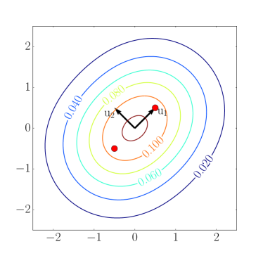
Figure 3: Level set of the density of the 2D Gaussian mixture. The red dots are the location of the means $a$ and $-a$, where $a$ is chosen such that $\left\|a\right\|_{2}^{2}=\frac{1}{2}$. The arrows indicate the two principal directions $u_{1}$ and $u_{2}$ along which the TV error is measured.

Note that one can sample directly from the mixture of Gaussian under consideration by drawing independently a Bernoulli$(1/2)$ random variable $y$ and a standard normal variable $z\sim\mathcal{N}(0,\mathbb{I}_{d})$, and then outputting the random variable

$$x=y\cdot(z-a)+(1-y)\cdot(z+a)$$

This observation makes it easy to diagnose the convergence of our Markov chains with target $\pi$. In order to estimate the total variation distance, we discretize the distribution of $N=250,000$ samples from $\pi$ over a set of bins, and consider the total variation of this discrete distribution from the empirical distribution of the Markov chain over these bins. We refer to this measure as the discretized TV error. We measure the sum of two discrete TV errors of $250,000$ samples from $\pi$ with the empirical distribution obtained by simulating the chains ULA, MALA or MRW, projected on two principal directions ($u_{1}$ and $u_{2}$), over a discrete grid of size $B=100$. Figure 4 shows the sum of the discretized TV errors along $u_{1}$ and $u_{2}$, as a function of iterations. The true total variation distance between the distribution of the iterate and the target distribution is upper bounded by the sum of (a) the discretized TV error and (b) the error caused by discretization. In order to obtain a sense of the magnitude of the error of type (b), we simulate $100$ runs of the discrete TV error between two independent drawings from the true distribution $\pi$. The two black lines in Figure 4 are the maximum and minimum of these $100$ values. The sample distribution at convergence is expected to lie between the two black lines.

Figure 4(a) shows that ULA converges significantly slower than MALA to the right distribution. Figure 4(b) illustrates this point further and shows that when compared to the ULA, the small-step ULA ($\delta=0.1$) converges at a much slower rate and large-step ULA ($\delta=1.0$) has a larger approximation error (asymptotic bias).

(a)	(b)

Figure 4: Discrete TV error on a two component Gaussian mixture. (a) Behavior of three different random walks. (b) Behavior of ULA with different choices of step sizes.

We accompany the study based on exact TV error computation with two classical convergence diagnostic plots for general MCMC algorithms. Figure 5 shows the trace plots of the three sampling algorithms in $10$ runs. Comparing the three panels (a)—(c) in Figure 5, we observe that the trace plot of MALA stabilizes much faster than that of ULA and MRW. Furthermore, to compare the efficiency of the chains in stationarity, Figure 6 shows the autocorrelation function of the three chains. In order to ensure that these autocorrelations are computed for the stationary distribution, we set in practice the burn-in period to be $300$ iterations. Again, we observe that MALA is more efficient than ULA and MRW.

(a)	(b)	(c)

Figure 5: Trace-plot of the first coordinate on a two component Gaussian mixture. (a) Trace-plot of ULA. (b) Trace-plot of MALA. (c) Trace-plot of MRW.

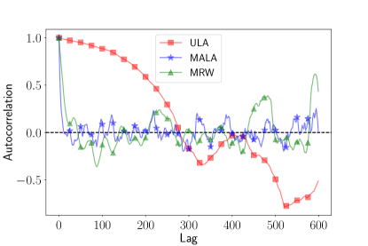
Figure 6: Markov chain autocorrelation function plot. The burn-in time for the plot is set to $300$ iterations.

4.3 Bayesian Logistic Regression

We now consider the problem of logistic regression in a frequentist-Bayesian setting, similar to that considered by Dalalyan (2016). Once again, we establish that MALA has superior performance relative to ULA. Given a binary variable $y\in\{0,1\}$ and a covariate $x\in{}^{d}$, the logistic model for the conditional distribution of $y$ given $x$ takes the form

$${\mathbb{P}}(y=1|x;\theta)=\frac{e^{\theta^{\top}x}}{1+e^{\theta^{\top}x}},$$ (20)

for some parameter $\theta\in{}^{d}$.

In a Bayesian framework, we model the parameter $\theta$ in the logistic equation as a random variable with a prior distribution $\pi_{0}$. Suppose that we observe a set of independent samples $\left\{(x_{i},y_{i})\right\}_{i=1}^{n}$ with $(x_{i},y_{i})\in{}^{d}\times\{0,1\}$, with each $y_{i}$ conditioned on $x_{i}$ drawn from a logistic distribution with some unknown parameter $\theta^{*}$. Using Bayes’ rule, we can then compute the posterior distribution of the parameter $\theta$ given the data. Drawing samples from this posterior distribution allows us to estimate and draw inferences about the unknown parameter. Under mild conditions, the Bernstein-von-Mises theorem guarantees that the posterior distribution will concentrate around the true parameter $\theta^{*}$, in which case we expect that the credible intervals formed by sampling from the posterior should contain $\theta^{*}$ with high probability. This fact provides a lens for us to assess the accuracy of our sampling procedure.

Define the vector $Y=\left(y_{1},\ldots,y_{n}\right)^{\top}\in\left\{0,1\right\}^{n}$ and let $X$ be the $n\times d$ matrix with $x_{i}$ as $i^{\text{th}}$-row. We choose the prior $\pi_{0}$ to be a Gaussian distribution with zero mean and covariance matrix proportional to the inverse of the sample covariance matrix $\Sigma_{X}=\frac{1}{n}X^{\top}X$. Plugging in the formulas for the prior and likelihood, we find that the the posterior density is given by

$$\pi(\theta)=\pi(\theta|X,Y)\propto\exp\left\{Y^{\top}X\theta-\sum_{i=1}^{n}\log\left(1+e^{\theta^{\top}x_{i}}\right)-\alpha\left\|\Sigma_{X}^{1/2}\theta\right\|_{2}^{2}\right\},$$

where $\alpha>0$ is a user-specified parameter. Writing $\pi\propto e^{-f}$, we observe that the function $f$ and its derivatives are given by

$$f(\theta) =-Y^{\top}X\theta+\sum_{i=1}^{n}\log\left(1+e^{\theta^{\top}x_{i}}\right)+\alpha\left\|\Sigma_{X}^{1/2}\theta\right\|_{2}^{2},$$

$$\nabla f(\theta) =-X^{\top}Y+\sum_{i=1}^{n}\frac{x_{i}}{1+e^{-\theta^{\top}x_{i}}}+\alpha\Sigma_{X}\theta,\quad\text{and},$$

$$\nabla^{2}f(\theta) =\sum_{i=1}^{n}\frac{e^{-\theta^{\top}x_{i}}}{\left(1+e^{-\theta^{\top}x_{i}}\right)^{2}}x_{i}x_{i}^{\top}+\alpha\Sigma_{X}.$$

With some algebra, we can deduce that the eigenvalues of the Hessian $\nabla^{2}f$ are bounded between $L:=\left(0.25n+\alpha\right)\,\lambda_{\text{max}}(\Sigma_{X})$ and $m:=\alpha\,\lambda_{\text{min}}(\Sigma_{X})$ where $\lambda_{\text{max}}(\Sigma_{X})$ and $\lambda_{\text{min}}(\Sigma_{X})$ denote the largest and smallest eigenvalues of the matrix $\Sigma_{X}$. We make use of these bounds in our experiments.

As in Dalalyan (2016), we also consider a preconditioned version of the method; more precisely, we first sample from $\pi_{g}\propto e^{-g}$ where $g(\theta)=f(\Sigma_{X}^{-1/2}\theta)$, and then transform the obtained random samples $\theta_{i}\mapsto\Sigma_{X}^{1/2}\theta_{i}$ to obtain samples from $\pi$. Sampling based on the preconditioned distribution improves the condition number of the problem. After the preconditioning, we have the bounds $L_{g}\leq 0.25n+\alpha$ and $m_{g}\geq\alpha$, so that the new condition number is now independent of the eigenvalues of $\Sigma_{X}$.

We randomly draw i.i.d. samples $\left(x_{i},y_{i}\right)$ as follows. Each vector $x_{i}\in{}^{d}$ is sampled i.i.d. Rademacher components, and then renormalized to Euclidean norm. given $x_{i}$, the response $y_{i}$ is drawn from the logistic model (20) with $\theta=\theta^{*}=\mathbf{1}_{d}=\left(1,\ldots,1\right)^{\top}$. We fix $d=2,n=50$ and perform $N=1000$ experiments. In order to sample from the posterior, we start with the initial distribution as $\mu_{0}=\mathcal{N}(0,L^{-1}\mathbb{I}_{d})$. As the first error metric, we measure the $\ell_{1}$-distance between the true parameter $\theta^{*}$ and the sample mean $\hat{\theta}_{k}$ of the random samples obtained from simulating the Markov chains for $k$ iterations:

$$e_{k}=\frac{1}{d}\|\hat{\theta}_{k}-\theta^{*}\|_{1}.$$

Figure 7 provides a log-scale plot of this error versus the iteration number. Since there is always an approximation error caused by the prior distribution, ULA with large step-size ($\delta=1.0$) can be used. However, our simulation shows that it is still slower than MALA. Also, the condition number $\kappa$ has a significant effect on the mixing time of ULA and MRW. Their convergence in the preconditioned case is significantly better. Furthermore, the autocorrelation plots in Figure 8 and the plots in Figure 9 of the sample (across experiments) mean and $25\%$ and $75\%$ quantiles, with $\theta^{*}$ subtracted, as a function of iterations suggest a similar story: MALA converges faster than ULA and is less affected by the conditioning of the problem.

(a)	(b)

Figure 7: Mean error as a function of iteration number. (a) Without preconditioning. (b) With preconditioning.

(a)	(b)

Figure 8: Autocorrelation function plot of the first coordinate of the estimate as a function lag. The burn-in time for the plot is set to 300 iterations. (a) Without preconditioning. (b) With preconditioning.

(a)	(b)

Figure 9: Mean and $25\%$ and $75\%$ quantiles, with $\theta^{*}$ subtracted, as a function of iteration number. (a) Without preconditioning. (b) With preconditioning.

4.4 Step size vs accept-reject rate

In this section, we provide a few simulations that highlight the effect of step size for MALA and MRW. Note that our bounds from Theorem 1 and 2 suggest a step size choice of order $d^{-1}$ for both MALA and MRW, which in turn led to the mixing time bounds of $\mathcal{O}\left(d\right)$. These choices of step sizes arise when we try to provide a worst-case control on the accept-reject step of these algorithms. In particular, these choices ensure that the Markov chains do not get stuck at a given state $x$, or equivalently, that the proposals at any given state are accepted with constant probability. If instead, one chooses a very large step size, the (worst-case) probability of acceptance may decay exponentially with dimensions. Nonetheless, these worst-case bounds may not hold, which would imply a faster mixing time for these chains if a larger step size were to be used.

To check the validity of larger step sizes, we repeated a few experiments discussed above, albeit with a larger step size. In particular, we simulated the random walks for a wide-range of step sizes $d^{-\gamma}$ for $\gamma\in\left\{0.2,0.33,0.5,0.67\right\}$ for MALA, and, $\gamma\in\left\{0.4,0.67,1,1.33\right\}$ for MRW. We ran these chains for two different cases: (a) Sampling from non-isotropic Gaussian density, discussed in Section 4.1, and, (b) Posterior sampling in Bayesian logistic regression, discussed in Section 4.3). In Figure 10, we plot the average acceptance probability for different step sizes $d^{-\gamma}$ as the dimension $d$ increases. These probabilities were computed as the average number of proposals accepted over $100$ iterations after a manually tuned burn-in period, and further averaged across $50$ independent runs.

(a) MALA: Non-isotropic Gaussian	(b) MALA: Bayesian logistic regression
(c) MRW: Non-isotropic Gaussian	(d) MRW: Bayesian logistic regression

Figure 10: Effect of large step size for accept-reject ratio for MALA and MRW. From panels (a) and (b), we see that for MALA the step size choice of $d^{-0.5}$ has a non-vanishing acceptance probability rate for both cases. On the other hand, panels (c) and (d) show that for MRW $d^{-1}$ is a good choice for the step size.

We now remark on the observations from Figure 10. We see that for MALA the acceptance probability for the step size choice of $d^{-0.2}$ vanishes as $d$ increases. Indeed, the choice of $d^{-0.5}$ appears to be a safe choice for both cases. In contrast, for MRW, we need a smaller step size. From panels (c) and (d), we see that $d^{-1}$ appears to be the correct choice to ensure that the proposals are accepted with a constant probability when the dimension $d$ is large.

Informally, if a step size choice of $d^{-\gamma}$ was to guarantee a non-vanishing acceptance probability for MALA or MRW, our proof techniques imply a mixing time bound of $\mathcal{O}\left(d^{\gamma}\right)$. Combining this argument with the observations above, we suspect that the bounds for MALA from Theorem 1 may not be tight, while for MRW the bounds from Theorem 2 are very likely to be tight. Deriving a faster mixing time for MALA or establishing that the current dimension dependency for MRW is tight, are interesting research directions and we leave the further investigation of these questions for future work.

5 Proofs

We now turn to the proofs of our main results. In Section 5.1, we begin by introducing some background on conductance bounds, before stating three auxiliary lemmas that underlie the proofs of our main theorems. Taking these three lemmas as given, we then provide the proof of Theorem 1 in Section 5.2. Sections 5.3 through 5.5 are devoted to the proofs of our three key lemmas, and we conclude with the proof of Theorem 2 in Section 5.6.

5.1 Conductance bounds and auxiliary results

Our proofs exploit standard conductance-based arguments for controlling mixing times. Consider an ergodic Markov chain defined by a transition operator $\mathcal{T}$, and let $\Pi$ be its stationary distribution. For each scalar $s\in(0,1/2)$, we define the $s$-conductance

$$\Phi_{s}:=\inf_{\Pi({A})\in(s,1-s)}\frac{\int_{{A}}\mathcal{T}_{u}({A}^{c})\pi(u)du}{\min\left\{\Pi({A})-s,\Pi({A}^{c})-s\right\}}.$$ (21)

In this formula, the notation $\mathcal{T}_{u}$ is shorthand for the distribution $\mathcal{T}(\mathbf{\delta}_{u})$ obtained by applying the transition operator to a dirac distribution concentrated on $u$. In words, the $s$-conductance measures how much probability mass flows across disjoint sets relative to their stationary mass. By a continuity argument, it can be seen that limiting conductance of the chain is equal to the limiting value of $s$-conductance—that is, $\Phi=\lim_{s\rightarrow 0}\Phi_{s}$.

For a reversible lazy Markov chain with $\beta$-warm start, Lovász 1999 (see also Kannan et al. (1995)) proved that

$$\|\mathcal{T}^{k}(\mu_{0})-\Pi\|_{\mbox{\tiny{TV}}}\leq\beta s+\beta\left(1-\frac{\Phi_{s}^{2}}{2}\right)^{k}\leq\beta s+{\beta}e^{-k{\Phi_{s}^{2}}/{2}}\quad\mbox{for any $s\in\big{(}0,\frac{1}{2}\big{)}$.}$$ (22)

In order to make effective use of this lower bound, we need to lower bound the $s$-conductance $\Phi_{s}$, and then choose the parameter $s$ so as to optimize the tradeoff between the two terms in the bound. We now state some auxiliary results that are useful.

We start with a result that shows that the probability mass of any strongly log concave distributions is concentrated in a Euclidean ball around the mode. For each $s\in(0,1)$, we introduce the Euclidean ball

$$\mathcal{R}_{s}=\mathbb{B}\left(x^{\star},r(s)\sqrt{\frac{d}{m}}\right)$$ (23)

where the function $r$ was previously defined in equation (9a), and $x^{\star}:=\arg\max\limits_{x\in{}^{d}}\pi(x)$ denotes the mode.

Lemma 1

For any $s\in\big{(}0,\frac{1}{2}\big{)}$, we have $\Pi(\mathcal{R}_{s})\geq 1-s$.

See Section 5.3 for the proof of this claim.

In order to establish the conductance bounds inside this ball, we first prove an extension of a result by Lovász (1999). The next result provides a lower bound on the flow of Markov chain with transition distribution $\mathcal{T}_{x}$ and strongly log concave target distributions $\Pi$. Similar results have been used in several prior works to establish fast mixing of several random walks like ball walk, Hit and run (Lovász, 1999; Lovász and Vempala, 2006, 2007), Dikin walk (Narayanan, 2016) and Vaidya and John walks (Chen et al., 2018).

Lemma 2

Let $\mathcal{K}$ be a convex set such that $\|\mathcal{T}_{x}-\mathcal{T}_{y}\|_{\mbox{\tiny{TV}}}\leq 1-\rho$ whenever $x,y\in\mathcal{K}$ and $\left\|x-y\right\|_{2}\leq\Delta$. Then for any measurable partition ${A}_{1}$ and ${A}_{2}$ of ^d, we have

$$\int_{{A}_{1}}\mathcal{T}_{u}({A}_{2})\pi(u)du\geq\frac{\rho}{4}\min\left\{1,\frac{\log 2\cdot\Delta\cdot\Pi^{2}(\mathcal{K})\cdot\sqrt{m}}{8}\right\}\min\left\{\Pi({A}_{1}\cap\mathcal{K}),\Pi({A}_{2}\cap\mathcal{K})\right\}.$$ (24)

See Section 5.4 for the proof of this lemma.

We next introduce a few pieces of notations to state a MALA specific result. Define a function $\tilde{w}:(0,1)\times(0,1)\rightarrow{}_{+}$ as follows:

$$\tilde{w}(s,\epsilon) :=\min\bigg{\{}\frac{\sqrt{\epsilon}}{8\sqrt{2}r(s)}\frac{\sqrt{m}}{L\sqrt{dL}},\frac{\epsilon}{64\alpha_{\epsilon}}\frac{1}{Ld},\frac{\epsilon^{2/3}}{26(\alpha_{\epsilon}r^{2}(s))^{1/3}}\frac{1}{L}\left(\frac{m}{Ld^{2}}\right)^{1/3}\bigg{\}},$$ (25a)

$$\text{where}\quad\alpha_{\epsilon} :=1+2\sqrt{\log(16/\epsilon)}+2\log(16/\epsilon),$$ (25b)

and the function $$r$$ was defined in equation (9a).

In the next lemma, we show two important properties for MALA: (1) the proposal distributions of MALA at two different points are close if the two points are close, and (2) the accept-reject step of MALA is well behaved inside the ball $\mathcal{R}_{s}$ provided the step size is chosen carefully. Note that for MALA, the proposal distribution of the chain at $x$ is given by

$$\mathcal{P}_{x}^{\text{\tiny MALA}(h)}=\mathcal{N}(\mu_{x},2h\mathbb{I}_{d}),\quad\text{where }\quad\mu_{x}=x-h\nabla f(x).$$ (26)

We use $\mathcal{T}_{x}^{\text{\tiny MALA}(h)}$ to denote the transition distribution of MALA.

Lemma 3

For any step size $$h\in\big{(}0,\frac{2}{L}\big{]}$$, the MALA proposal distribution satisfies the bound

$$\sup_{\begin{subarray}{c}x,y\in{}^{d}\\ x\neq y\end{subarray}}\frac{\|\mathcal{P}_{x}^{\text{\tiny MALA}(h)}-\mathcal{P}_{y}^{\text{\tiny MALA}(h)}\|_{\mbox{\tiny{TV}}}}{\left\|x-y\right\|_{2}} \leq\frac{1}{\sqrt{2h}}.$$ (27a)

Moreover, given scalars $$s\in(0,1/2) \epsilon\in(0,1) h\in\big{(}0,\tilde{w}(s,\epsilon)\big{]}$$ and , then the MALA proposal distribution for any step size satisfies the bound

$$\sup_{x\in\mathcal{R}_{s}}\|\mathcal{P}_{x}^{\text{\tiny MALA}(h)}-\mathcal{T}_{x}^{\text{\tiny MALA}(h)}\|_{\mbox{\tiny{TV}}}\leq\frac{\epsilon}{8},$$ (27b)

where the truncated ball $$\mathcal{R}_{s}$$ was defined in equation (23).

See Section 5.5 for the proof of this claim. With these results in hand, we are now equipped to prove the mixing time bound for MALA.

5.2 Proof of Theorem 1

At a high level, the proof involves three key steps. Our first step is to use Lemma 3 to establish that for an appropriate choice of step size, the MALA update has nice properties inside a high probability region given by Lemma 1. The second step is to apply Lemma 2 so as to obtain a lower bound on the $s$-conductance $\Phi_{s}$ of the MALA update. Finally, by making an appropriate choice of parameter $s$, we establish the claimed convergence rate.

In order to simplify notation, we drop the superscripts $\text{\tiny MALA}(h)$ from our notation—that is, we use $\mathcal{T}_{x}$ and $\mathcal{P}_{x}$, respectively, to denote the transition and proposal distributions at $x$ for MALA, each with step size $h$. By applying the triangle inequality, we obtain the upper bound

$$\|\mathcal{T}_{x}-\mathcal{T}_{y}\|_{\mbox{\tiny{TV}}}\leq\|\mathcal{P}_{x}-\mathcal{T}_{x}\|_{\mbox{\tiny{TV}}}+\|\mathcal{P}_{x}-\mathcal{P}_{y}\|_{\mbox{\tiny{TV}}}+\|\mathcal{P}_{y}-\mathcal{T}_{y}\|_{\mbox{\tiny{TV}}}.$$ (28)

Now applying claim (27a) from Lemma 3 guarantees that

$$\|\mathcal{P}_{x}-\mathcal{P}_{y}\|_{\mbox{\tiny{TV}}}\leq\epsilon/\sqrt{2}\qquad\mbox{ for all $x,y\in{}^{d}$ such that $\left\|x-y\right\|_{2}\leq\epsilon\sqrt{h}$.}$$

Furthermore, for any $h\leq\tilde{w}(s,\epsilon)$, the bound (27b) from Lemma 3 implies that $\|\mathcal{P}_{x}-\mathcal{T}_{x}\|_{\mbox{\tiny{TV}}}\leq\epsilon/8$ for any $x\in\mathcal{R}_{s}$. Plugging in these bounds in the inequality (28), we find that

$$\|\mathcal{T}_{x}-\mathcal{T}_{y}\|_{\mbox{\tiny{TV}}}\leq 1-(1-\epsilon)\quad\mbox{ $\forall\ x,y\in\mathcal{R}_{s}$ such that $\left\|x-y\right\|_{2}\leq\epsilon\sqrt{h}$.}$$

Thus, the transition distribution $\mathcal{T}_{x}$ satisfies the assumptions of Lemma 2 for

$$\mathcal{K}=\mathcal{R}_{s},\quad\rho=(1-\epsilon)\quad\text{ and }\quad\Delta=\epsilon\sqrt{h}.$$ (29)

We now derive a lower bound on the $s$-conductance of MALA. Choosing a measurable set ${A}$ such that $\Pi({A})>s$ and substituting the terms from equation (29) in the inequality (24), we find that

$$\int_{{A}}\mathcal{T}_{u}({A}^{c})\pi(u)du \geq\frac{(1-\epsilon)}{4}\min\left\{1,\frac{\log 2\cdot\epsilon\sqrt{h}\cdot\Pi^{2}(\mathcal{R}_{s})\cdot\sqrt{m}}{8}\right\}\cdot$$

$$\quad\quad\quad\cdot\min\left\{\Pi({A}\cap\mathcal{R}_{s}),\Pi({A}^{c}\cap\mathcal{R}_{s})\right\}$$

$$\stackrel{{\scriptstyle(i)}}{{\geq}}\frac{(1-\epsilon)\epsilon\sqrt{h}\cdot\Pi^{2}(\mathcal{R}_{s})\cdot\sqrt{m}}{64}\min\left\{\Pi({A})-s,\Pi({A}^{c})-s\right\}.$$

In this argument, inequality (i) follows from the facts that $\log 2\geq 1/2$ and $\Pi({A}),\Pi({A}^{c})>s$. Moreover, we have applied Lemma 1 to find that $\Pi(\mathcal{R}_{s})\geq 1-s$ and hence

$$\Pi(\mathcal{X}\cap\mathcal{R}_{s})=\Pi(\mathcal{X})-\Pi(\mathcal{X}\cap\mathcal{R}_{s}^{c})\geq\Pi(\mathcal{X})-s\quad\mbox{for $\mathcal{X}\in\left\{{A},{A}^{c}\right\}$.}$$

We have also assumed that the second argument of the minimum is less than $1$. Applying the definition (21) of $\Phi_{s}$ for MALA, we find that

$$\Phi_{s}^{\text{\tiny MALA}\footnotesize{(h)}}\geq\frac{(1-\epsilon)\epsilon\cdot\Pi^{2}(\mathcal{R}_{s})\cdot\sqrt{hm}}{64},\quad\text{ for any }h\leq\tilde{w}(s,\epsilon).$$ (30)

By making a suitable choice of $s$, we can now complete the proof. Using Lemma 1, we have that $\Pi(\mathcal{R}_{\delta/2})\geq 1-\delta/2\geq 1/2$ for any $\delta\in(0,1)$. Applying the definition (25b) of $\alpha_{\epsilon}$, we obtain that $\alpha_{1/2}\leq 12$. Using this fact and the definitions (9b) and (25a) for the functions $w(\cdot)$ and $\tilde{w}(\cdot,\cdot)$, it is straightforward to verify that $cw(\delta/(2\beta))\leq\tilde{w}(\delta/(2\beta),1/2)$, for an appropriate choice of universal constant $c$. Substituting in $s=\delta/(2\beta)$, $\epsilon=1/2$, and $h=cw(\delta/(2\beta))$, and also making use of the lower bound $\Pi(\mathcal{R}_{\delta/2\beta})\geq 1/2$ in the bound (30), we find that $\Phi_{\delta/2\beta}^{\text{\tiny MALA}\footnotesize{(h)}}\geq c^{\prime}\sqrt{mh}$ for some universal constant $c^{\prime}$. Using the convergence rate (22), we obtain that

$$\|\mathcal{T}_{\text{\tiny MALA}(h)}^{k}(\mu_{0})-\Pi\|_{\mbox{\tiny{TV}}}\leq\beta\frac{\delta}{2\beta}+{\beta}e^{-kmh/c^{\prime}}\leq\delta\quad\text{ for all }\quad k\geq\frac{c^{\prime}}{mh}\cdot\log\left(\frac{2{\beta}}{\delta}\right),$$ (31)

for a suitably large constant $c^{\prime}$. Substituting the expression (9b) for $h=cw(\delta/(2\beta))$, yields the claimed bound on mixing time.

5.3 Proof of Lemma 1

The proof consists of two main steps. First, we establish that the distribution $\Pi$ is sub-Gaussian, which then guarantees concentration around the mean. Second, we show that the mean and the mode of the distribution $\Pi$ are not far apart. Combining these two claims yields a high probability region around the mode $x^{\star}$.

Let $x$ denote the random variable with distribution $\Pi$ and mean $\bar{x}={\mathbb{E}}_{x\sim\Pi}\left[x\right]$. We claim that $x-\bar{x}$ is a sub-Gaussian random vector with parameter $1/\sqrt{m}$, meaning that

$${\mathbb{E}}_{x}\left[e^{u^{\top}(x-\bar{x})}\right]\leq e^{{\left\|u\right\|_{2}^{2}}/(2m)}\quad\text{ for any vector }u\in{}^{d}.$$

In order to prove this claim, we make use of a result due to Hargé (2004) (Theorem 1.1), which we restate here. Let $y\sim\mathcal{N}(\mu,\Sigma)$ with density $e$ and $x$ be a random variable with density function $q\cdot e$ where $q$ is a log-concave function. Then for any convex function $g:{}^{d}\mapsto\real$ we have

$${\mathbb{E}}_{x}\left[g(x-{\mathbb{E}}[x])\right]\leq{\mathbb{E}}_{y}\left[g(y-{\mathbb{E}}[y])\right].$$ (32)

From Lemma 4(b) we have that $x\mapsto f(x)-\frac{m}{2}\left\|x-x^{\star}\right\|_{2}^{2}$ is a convex function. Thus we can express the density $\pi$ as the product of a log concave function and the density of a random variable with distribution $\mathcal{N}(x^{\star},\mathbb{I}_{d}/m)$. Letting $y\sim\mathcal{N}(x^{\star},\mathbb{I}_{d}/m)$ and noting that $g(z):=e^{u^{\top}z}$ is a convex function for each fixed vector $u$, applying the Hargé bound (32) yields

$${\mathbb{E}}_{x}\left[e^{u^{\top}(x-\bar{x})}\right]\leq{\mathbb{E}}_{y}\left[e^{u^{\top}(y-x^{*})}\right]\stackrel{{\scriptstyle(i)}}{{\leq}}e^{\left\|u\right\|_{2}^{2}/2m}.$$

Here inequality (i) follows from the fact that the random vector $y-x^{\star}$ is sub-Gaussian with parameter $1/\sqrt{m}$.

Using the standard tail bounds for quadratic forms for sub-Gaussian random vectors (e.g., Theorem 1 by Hsu et al. 2012), we find that

$${\mathbb{P}}_{x\sim\Pi}\left[\left\|x-\bar{x}\right\|_{2}^{2}>\frac{d}{m}\left(1+2\sqrt{\frac{t}{d}}+2\frac{t}{d}\right)\right]\leq e^{-t}.$$ (33)

Define $\mathcal{B}_{1}:=\mathbb{B}\left(\bar{x},\sqrt{\frac{d}{m}}\cdot\tilde{r}(s)\right)$ where $\tilde{r}(s)=1+2\max\left\{\left(\frac{\log(1/s)}{d}\right)^{0.25},\sqrt{\frac{\log(1/s)}{d}}\right\}$. Observe that $\tilde{r}(s)^{2}\ {\geq}\ {{1+2\sqrt{\frac{\log(1/s)}{d}}+2\frac{\log(1/s)}{d}}}$ and consequently the bound (33) implies that $\Pi\left(\mathcal{B}_{1}\right)={\mathbb{P}}_{x\sim\Pi}\left[x\in\mathcal{B}_{1}\right]\geq 1-s$. Now applying triangle inequality, we obtain that

$$\mathcal{B}_{1}\subseteq\mathbb{B}\left(x^{\star},\left\|\bar{x}-x^{\star}\right\|_{2}+\sqrt{\frac{d}{m}}\cdot\tilde{r}(s)\right)=:\mathcal{B}_{2}$$

From Theorem 1 by Durmus et al. (2019), we have that ${\mathbb{E}}_{x\sim\Pi}\left\|x-x^{\star}\right\|_{2}^{2}\leq{d/m}$. Using Jensen inequality twice, we find that

$${\left\|\bar{x}-x^{\star}\right\|_{2}}=\left\|{\mathbb{E}}_{x\sim\Pi}\left[x\right]-x^{\star}\right\|_{2}\leq{{\mathbb{E}}_{x\sim\Pi}\left\|x-x^{\star}\right\|_{2}}\leq\sqrt{{\mathbb{E}}_{x\sim\Pi}\left\|x-x^{\star}\right\|_{2}^{2}}\leq\sqrt{\frac{d}{m}}.$$ (34)

Noting the relation $r(s)=1+\tilde{r}(s)$, we thus obtain that $\left\|\bar{x}-x^{\star}\right\|_{2}+\sqrt{\frac{d}{m}}\cdot\tilde{r}(s)\leq r(s)\sqrt{\frac{d}{m}}$ and consequently $\mathcal{B}_{1}\subseteq\mathcal{B}_{2}\subseteq\mathcal{R}_{s}$. As a result, we obtain $\Pi\left(\mathcal{R}_{s}\right)\geq\Pi\left(\mathcal{B}_{1}\right)\geq 1-s$ as claimed.

5.4 Proof of Lemma 2

The proof of this lemma is based on the ideas employed in prior works to establish conductance bounds, first for Hit-and-run (Lovász, 1999), and since then for several other random walks (Lovász and Vempala, 2007; Narayanan, 2016; Chen et al., 2018). See the survey by Vempala (2005) for further details.

For our setting, a key ingredient is the following isoperimetric inequality for log-concave distributions. Let ${}^{d}={S}_{1}\cup{S}_{2}\cup{S}_{3}$ be a partition. Let $y\sim\mathcal{N}(0,\sigma^{2}\mathbb{I}_{d})$ with density $e$ and let $\Pi$ be a distribution with a density given by $q\cdot e$ where $q$ is a log-concave function. Then Cousins and Vempala (2014) (Theorem 4.4) proved that

$$\Pi({S}_{3})\geq\frac{\log 2\cdot d({S}_{1},{S}_{2})}{\sigma}\Pi({S}_{1})\Pi({S}_{2})$$ (35)

where $d({S}_{1},{S}_{2}):=\inf\left\{\left\|x-y\right\|_{2}\big{|}x\in{S}_{1},y\in{S}_{2}\right\}$.

We invoke this result for the truncated distribution $\Pi_{\mathcal{K}}$ with the density $\pi_{\mathcal{K}}$ defined as

$$\pi_{\mathcal{K}}(x):=\frac{1}{\displaystyle\int_{\mathcal{K}}\pi(y)dy}\pi(x)\mathbbm{1}_{\mathcal{K}}(x)=\frac{1}{\displaystyle\int_{\mathcal{K}}e^{-f(y)}dy}e^{-f(x)}\mathbbm{1}_{\mathcal{K}}(x),$$ (36)

where $\mathbbm{1}_{\mathcal{K}}(\cdot)$ denotes the indicator function for the set $\mathcal{K}$, i.e., we have $\mathbbm{1}_{\mathcal{K}}(x)=1$ if $x\in\mathcal{K}$, and $0$ otherwise. Let $x^{\star}=\arg\max\pi(x)=\arg\min f(x)$. Observe that $m$-strong-convexity of $f$ implies that $x\mapsto f(x)-\frac{m}{2}\left\|x-x^{\star}\right\|_{2}^{2}$ is a convex function (Lemma 4(b)). Noting that the function $\mathbbm{1}_{\mathcal{K}}(\cdot)$ is log-concave and that log-concavity is closed under multiplication, we conclude that $\pi_{\mathcal{K}}$ can be expressed as a product of log-concave function and density of the Gaussian distribution $\mathcal{N}\left(x^{\star},\frac{1}{m}\mathbb{I}_{d}\right)$. Consequently, we can apply the result (35) with $\Pi$ replaced by $\Pi_{\mathcal{K}}$ and $\sigma=1/\sqrt{m}$.

We now prove the claim of the lemma. Define the sets

$${A}_{1}^{\prime}:=\left\{u\in{A}_{1}\cap\mathcal{K}\;\mid\;\mathcal{T}_{u}({A}_{2})<\frac{\rho}{2}\!\right\},\quad{A}_{2}^{\prime}:=\left\{v\in{A}_{2}\cap\mathcal{K}\;\mid\;\mathcal{T}_{v}({A}_{1})<\frac{\rho}{2}\right\},$$ (37)

along with the complement ${A}_{3}^{\prime}:=\mathcal{K}\backslash({A}_{1}^{\prime}\cup{A}_{2}^{\prime})$. See Figure 11 for an illustration. Based on these three sets, we split our proof of the claim (24) into two distinct cases:

• Case 1: $\Pi({A}_{1}^{\prime})\leq\Pi({A}_{1}\cap\mathcal{K})/2$ or $\Pi({A}_{2}^{\prime})\leq\Pi({A}_{2}\cap\mathcal{K})/2$.

• Case 2: $\Pi({A}_{i}^{\prime})\geq\Pi({A}_{i}\cap\mathcal{K})/2$ for $i=1,2$.

Note that these cases are mutually exclusive, and cover all possibilities.

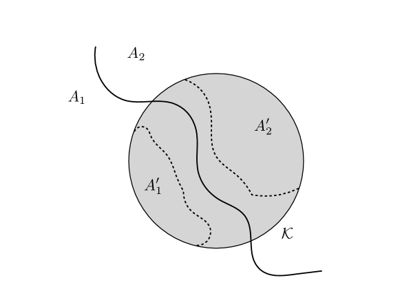
Figure 11: The sets ${A}_{1}$ and ${A}_{2}$ form a partition of ^d, and we use $\mathcal{K}$ to denote a compact convex subset. The sets ${A}_{1}^{\prime}$ and ${A}_{2}^{\prime}$ are defined in equation (37).

Case 1

We have $\Pi({A}_{1}\cap\mathcal{K}\backslash{A}_{1}^{\prime})\geq\Pi({A}_{1}\cap\mathcal{K})/2$, then

$$\int_{{A}_{1}}\mathcal{T}_{u}({A}_{2})\pi(u)du\stackrel{{\scriptstyle(i)}}{{\geq}}\int_{{A}_{1}\cap\mathcal{K}\backslash{A}_{1}^{\prime}}\mathcal{T}_{u}({A}_{2})\pi(u)du \stackrel{{\scriptstyle(ii)}}{{\geq}}\frac{\rho}{2}\Pi({A}_{1}\cap\mathcal{K}\backslash{A}_{1}^{\prime})$$

$$\stackrel{{\scriptstyle(iii)}}{{\geq}}\frac{\rho}{4}\Pi({A}_{1}\cap\mathcal{K}),$$

which implies the claim (24). In the above sequence of inequalities, step (i) is trivially true; step (ii) from the definition (37) of the set ${A}_{1}^{\prime}$, and step (iii) from the assumption for this case.

A similar argument with the roles of ${A}_{1}$ and ${A}_{2}$ switched, establishes the claim when $\Pi({A}_{2}^{\prime})\leq\Pi({A}_{2}\cap\mathcal{K})/2$.

Case 2

We have $\Pi({A}_{i}^{\prime})\geq\Pi({A}_{i}\cap\mathcal{K})/2$ for both $i=1$ and $2$. For any $u\in{A}_{1}^{\prime}$ and $v\in{A}_{2}^{\prime}$, we have that

$$\|\mathcal{T}_{u}-\mathcal{T}_{v}\|_{\mbox{\tiny{TV}}}\geq\mathcal{T}_{u}({A}_{1})-\mathcal{T}_{v}({A}_{1})\stackrel{{\scriptstyle(i)}}{{=}}1-\mathcal{T}_{u}({A}_{2})-\mathcal{T}_{v}({A}_{1})>1-\rho,$$

where step (i) follows from the fact that ${A}_{1}={}^{d}\backslash{A}_{2}$ and thereby $\mathcal{T}_{u}({A}_{1})=1-\mathcal{T}_{u}({A}_{2})$. Since $u,v\in\mathcal{K}$, the assumption of the lemma implies that $\left\|u-v\right\|_{2}\geq\Delta$ and consequently

$$d({A}_{1}^{\prime},{A}_{2}^{\prime})\geq\Delta.$$ (38)

We claim that

$$\int_{{A}_{1}}\mathcal{T}_{u}({A}_{2})\pi(u)du=\int_{{A}_{2}}\mathcal{T}_{v}({A}_{1})\pi(v)dv$$ (39)

We provide the proof of this claim at the end. Assuming this claim as given, we now complete the proof. Using equation (39), we have

$$\int_{{A}_{1}}\mathcal{T}_{u}({A}_{2})\pi(u)du =\frac{1}{2}\left(\int_{{A}_{1}}\mathcal{T}_{u}({A}_{2})\pi(u)du+\int_{{A}_{2}}\mathcal{T}_{v}({A}_{1})\pi(v)dv\right)$$

$$\geq\frac{1}{4}\left(\int_{{A}_{1}\cap\mathcal{K}\backslash{A}_{1}^{\prime}}\mathcal{T}_{u}({A}_{2})\pi(u)du+\int_{{A}_{2}\cap\mathcal{K}\backslash{A}_{2}^{\prime}}\mathcal{T}_{v}({A}_{1})\pi(v)dv\right)$$

$$\stackrel{{\scriptstyle(i)}}{{\geq}}\frac{\rho}{8}\Pi(\mathcal{K}\backslash({A}_{1}^{\prime}\cup{A}_{2}^{\prime})),$$ (40)

where step (i) follows from the definition (37) of the set ${A}_{3}^{\prime}=\mathcal{K}\backslash({A}_{1}^{\prime}\cup{A}_{2}^{\prime})$. Further, we have

$$\Pi(\mathcal{K}\backslash({A}_{1}^{\prime}\cup{A}_{2}^{\prime})) \stackrel{{\scriptstyle(i)}}{{=}}\Pi(\mathcal{K})\cdot\Pi_{\mathcal{K}}(\mathcal{K}\backslash{A}_{1}^{\prime}\backslash{A}_{2}^{\prime})$$

$$\stackrel{{\scriptstyle(ii)}}{{\geq}}\Pi(\mathcal{K})\cdot\frac{\log 2\cdot d({A}_{1}^{\prime},{A}_{2}^{\prime})}{1/\sqrt{m}}\cdot\Pi_{\mathcal{K}}({A}_{1}^{\prime})\cdot\Pi_{\mathcal{K}}({A}_{2}^{\prime})$$

$$\stackrel{{\scriptstyle(iii)}}{{\geq}}\Pi(\mathcal{K})\cdot\log 2\cdot d({A}_{1}^{\prime},{A}_{2}^{\prime})\cdot\sqrt{m}\cdot\Pi({A}_{1}^{\prime})\cdot\Pi({A}_{2}^{\prime})$$

$$\stackrel{{\scriptstyle(iv)}}{{\geq}}\Pi(\mathcal{K})\cdot\log 2\cdot\Delta\cdot\sqrt{m}\cdot\frac{1}{4}\cdot\Pi({A}_{1}\cap\mathcal{K})\cdot\Pi({A}_{2}\cap\mathcal{K}).$$ (41)

where step (i) follows from the definition (36) of the truncated distribution $\Pi_{\mathcal{K}}$, step (ii) follows from applying the isoperimetry (35) for the distribution $\Pi_{\mathcal{K}}$ with $\sigma=1/\sqrt{m}$, step (iii) from the definition of $\Pi_{\mathcal{K}}$ and step (iv) from inequality (38) and the assumption for this case. Let $\alpha:=\Pi({A}_{1}\cap\mathcal{K})/\Pi(\mathcal{K})$. Note that $\alpha\in[0,1]$ and $\Pi({A}_{2}\cap\mathcal{K})/\Pi(\mathcal{K})=1-\alpha$. We have

$$\Pi({A}_{1}\cap\mathcal{K})\cdot\Pi({A}_{2}\cap\mathcal{K}) =\Pi^{2}(\mathcal{K})\cdot\alpha(1-\alpha)$$

$$\geq\Pi^{2}(\mathcal{K})\cdot\frac{1}{2}\min\left\{\alpha,1-\alpha\right\}$$

$$=\Pi(\mathcal{K})\cdot\frac{1}{2}\min\left\{\Pi({A}_{1}\cap\mathcal{K}),\Pi({A}_{2}\cap\mathcal{K})\right\}$$ (42)

Putting the inequalities (40), (41) and (42) together, establishes the claim (24) of the lemma for this case.

We now prove our earlier claim (39). Note that it suffices to prove that

$$\int_{{A}_{1}}\mathcal{T}_{u}({A}_{2})\pi(u)du=\int_{{A}_{2}}\mathcal{T}_{v}({A}_{1})\pi(v)dv.$$

We have

$$\int_{{A}_{2}}\mathcal{T}_{u}({A}_{1})\pi(u)du \stackrel{{\scriptstyle\mathmakebox[\widthof{==}]{(i)}}}{{=}}\int_{{}^{d}}\mathcal{T}_{u}({A}_{1})\pi(u)du-\int_{{A}_{1}}\mathcal{T}_{u}({A}_{1})\pi(u)du$$

$$\stackrel{{\scriptstyle\mathmakebox[\widthof{==}]{(ii)}}}{{=}}\Pi({A}_{1})-\int_{{A}_{1}}\mathcal{T}_{u}({A}_{1})\pi(u)du$$

$$\stackrel{{\scriptstyle\mathmakebox[\widthof{==}]{}}}{{=}}\int_{{A}_{1}}\pi(u)du-\int_{{A}_{1}}\mathcal{T}_{u}({A}_{1})\pi(u)du$$

$$\stackrel{{\scriptstyle\mathmakebox[\widthof{==}]{(iii)}}}{{=}}\int_{{A}_{1}}\mathcal{T}_{u}({A}_{2})\pi(u)du,$$

where steps (i) and (iii) (respectively) follow from the fact that ${A}_{1}={}^{d}\backslash{A}_{2}$ and the consequent fact that $1-\mathcal{T}_{u}({A}_{1})=\mathcal{T}_{u}({A}_{2})$, and step (ii) follows from the fact that $\pi$ is the stationary density for the transition distribution $\mathcal{T}_{x}$ and thereby $\int_{{}^{d}}\mathcal{T}_{u}({A}_{1})\pi(u)du=\Pi({A}_{1})$.

5.5 Proof of Lemma 3

We prove each claim of the lemma separately. To simplify notation, we drop the superscript from our notations of distributions $\mathcal{T}_{x}^{\text{\tiny MALA}(h)}$ and $\mathcal{P}_{x}^{\text{\tiny MALA}(h)}$.

5.5.1 Proof of claim (27a)

In order to bound the total variation distance $\|\mathcal{P}_{x}-\mathcal{P}_{y}\|_{\mbox{\tiny{TV}}}$, we apply Pinsker’s inequality (Cover and Thomas, 1991), which guarantees that $\|\mathcal{P}_{x}-\mathcal{P}_{y}\|_{\mbox{\tiny{TV}}}\leq\sqrt{2\operatorname{KL}(\mathcal{P}_{x}\|\mathcal{P}_{y})}$. Given multivariate normal distributions $\mathcal{G}_{1}=\mathcal{N}\left(\mu_{1},\Sigma\right)$ and $\mathcal{G}_{2}=\mathcal{N}\left(\mu_{2},\Sigma\right)$, the Kullback-Leibler divergence between the two is given by

$$\operatorname{KL}(\mathcal{G}_{1}\|\mathcal{G}_{2})=\frac{1}{2}\left(\mu_{1}-\mu_{2}\right)^{\top}\Sigma^{-1}\left(\mu_{1}-\mu_{2}\right).$$ (43)

Substituting $\mathcal{G}_{1}=\mathcal{P}_{x}$ and $\mathcal{G}_{2}=\mathcal{P}_{y}$ into the above expression and applying Pinsker’s inequality, we find that

$$\|\mathcal{P}_{x}-\mathcal{P}_{y}\|_{\mbox{\tiny{TV}}}\leq\sqrt{2\operatorname{KL}(\mathcal{P}_{x}\|\mathcal{P}_{y})} =\frac{\left\|\mu_{x}-\mu_{y}\right\|_{2}}{\sqrt{2h}}$$

$$\stackrel{{\scriptstyle(i)}}{{=}}\frac{\left\|(x-h\nabla f(x))-(y-h\nabla f(y))\right\|_{2}}{\sqrt{2h}},$$

where step (i) follows from the definition (26) of the mean $\mu_{x}$. Consequently, in order to establish the claim (27a), it suffices to show that

$$\left\|(x-h\nabla f(x))-(y-h\nabla f(y))\right\|_{2}\leq\left\|x-y\right\|_{2}.$$

Recalling that $|\!|\!|B|\!|\!|_{{\tiny{\mbox{op}}}}$ denotes the $\ell_{2}$-operator norm of a matrix $B$ (equal to the maximum singular value), we have

$$\left\|(x-h\nabla f(x))-(y-h\nabla f(y))\right\|_{2} =\left\|\int_{0}^{1}\left[\mathbb{I}-h\nabla^{2}f(x+t(x-y))\right](x-y)dt\right\|_{2}$$

$$\leq\int_{0}^{1}\left\|\left[\mathbb{I}-h\nabla^{2}f(x+t(x-y))\right](x-y)\right\|_{2}dt$$

$$\stackrel{{\scriptstyle(i)}}{{\leq}}\sup_{z\in{}^{d}}|\!|\!|\mathbb{I}_{d}-h\nabla^{2}f(z)|\!|\!|_{{\tiny{\mbox{op}}}}\;\left\|x-y\right\|_{2},$$

where step (i) follows from the definition of the operator norm. Lemma 4(f) and Lemma 5(f) guarantee that the Hessian is sandwiched as $m\mathbb{I}_{d}\preceq\nabla^{2}f(z)\preceq L\mathbb{I}_{d}$ for all $z\in{}^{d}$, where $\mathbb{I}_{d}$ denotes the $d$-dimensional identity matrix. From this Hessian sandwich, it follows that

$$|\!|\!|\mathbb{I}_{d}-h\nabla^{2}f(x)|\!|\!|_{{\tiny{\mbox{op}}}}=\max\left\{\left|1-hL\right|,\left|1-hm\right|\right\}\;<\;1.$$

Putting together the pieces yields the claim.

5.5.2 Proof of claim (27b)

Let $\mathcal{P}_{1}$ be a distribution admitting a density $p_{1}$ on ^d, and let $\mathcal{P}_{2}$ be a distribution which has an atom at $x$ and admitting a density $p_{2}$ on ${}^{d}\backslash\left\{x\right\}$. The total variation distance between the distributions $\mathcal{P}_{1}$ and $\mathcal{P}_{2}$ is given by

$$\|\mathcal{P}_{1}-\mathcal{P}_{2}\|_{\mbox{\tiny{TV}}}=\frac{1}{2}\left(\mathcal{P}_{2}(\left\{x\right\})+\int_{{}^{d}}\left|p_{1}(z)-p_{2}(z)\right|dz\right).$$ (44)

The accept-reject step for MALA implies that

$$\mathcal{T}_{x}(\left\{x\right\})=1-\int_{{}^{d}}\min\left\{1,\frac{\pi(z)\cdot p_{z}(x)}{\pi(x)\cdot p_{x}(z)}\right\}p_{x}(z)dz,$$ (45)

where $p_{x}$ denotes the density corresponding to the proposal distribution $\mathcal{P}_{x}=\mathcal{N}(x-h\nabla f(x),2h\mathbb{I}_{d})$. From this fact and the formula (44), we find that

$$\|\mathcal{P}_{x}-\mathcal{T}_{x}\|_{\mbox{\tiny{TV}}} =\frac{1}{2}\left(\mathcal{T}_{x}(\left\{x\right\})+\int_{{}^{d}}p_{x}(z)dz-\int_{{}^{d}}\min\left\{1,\frac{\pi(z)\cdot p_{z}(x)}{\pi(x)\cdot p_{x}(z)}\right\}p_{x}(z)dz\right)$$

$$=\frac{1}{2}\left(2-2\int_{{}^{d}}\min\left\{1,\frac{\pi(z)\cdot p_{z}(x)}{\pi(x)\cdot p_{x}(z)}\right\}p_{x}(z)dz\right)$$

$$=1-{\mathbb{E}}_{z\sim\mathcal{P}_{x}}\left[\min\left\{1,\frac{\pi(z)\cdot p_{z}(x)}{\pi(x)\cdot p_{x}(z)}\right\}\right].$$ (46)

By applying Markov’s inequality, we obtain

$${\mathbb{E}}_{z\sim\mathcal{P}_{x}}\left[\min\left\{1,\frac{\pi(z)\cdot p_{z}(x)}{\pi(x)\cdot p_{x}(z)}\right\}\right]\geq\alpha\;{\mathbb{P}}\left[\frac{\pi(z)\cdot p_{z}(x)}{\pi(x)\cdot p_{x}(z)}\geq\alpha\right]\quad\mbox{for all $\alpha\in(0,1]$}.$$ (47)

We now derive a high probability lower bound for the ratio $\left[\pi(z)p_{z}(x)\right]/\left[\pi(x)p_{x}(z)\right]$. Noting that $\pi(x)\propto\exp(-f(x))$ and $p_{x}(z)\propto\exp\left(-\left\|x-h\nabla f(x)-z\right\|_{2}^{2}/(4h)\right)$, we have

$$\displaystyle\frac{\pi(z)\cdot p_{z}(x)}{\pi(x)\cdot p_{x}(z)} =\frac{\exp\bigg{(}-f(z)-\frac{\left\|x-z+h\nabla f(z)\right\|_{2}^{2}}{4h}\bigg{)}}{\exp\bigg{(}-f(x)-\frac{\left\|z-x+h\nabla f(x)\right\|_{2}^{2}}{4h}\bigg{)}}$$

$$={\exp\bigg{(}\frac{4h(f(x)-f(z))+\left\|z-x+h\nabla f(x)\right\|_{2}^{2}-\left\|x-z+h\nabla f(z)\right\|_{2}^{2}}{4h}\bigg{)}}.$$ (48)

Keeping track of the numerator of this exponent, we find that

$$4h(f(x)-f(z))+\left\|z-x+h\nabla f(x)\right\|_{2}^{2}-\left\|x-z+h\nabla f(z)\right\|_{2}^{2}$$

$$\quad=4h(f(x)-f(z))+\left\|z-x\right\|_{2}^{2}+\left\|h\nabla f(x)\right\|_{2}^{2}+2h(z-x)^{\top}\nabla f(x)$$

$$\quad\quad\quad-\left\|x-z\right\|_{2}^{2}-\left\|h\nabla f(z)\right\|_{2}^{2}-2h(x-z)^{\top}\nabla f(z)$$

$$\quad=2h\underbrace{(f(x)-f(z)-(x-z)^{\top}\nabla f(x))}_{M_{1}}+2h\underbrace{(f(x)-f(z)-(x-z)^{\top}\nabla f(z))}_{M_{2}}$$

$$\quad\quad\quad+h^{2}\underbrace{\left(\left\|\nabla f(x)\right\|_{2}^{2}-\left\|\nabla f(z)\right\|_{2}^{2}\right)}_{M_{3}}.$$ (49)

Now we provide lower bounds for the terms $M_{i}$, $i=1,2,3$ defined in the above display. Since $f$ is strongly convex and smooth, applying Lemma 4(c) and Lemma 5(c) yields

$$M_{1}\geq-\frac{L}{2}\left\|x-z\right\|_{2}^{2},\quad\text{and}\quad M_{2}\geq\frac{m}{2}\left\|x-z\right\|_{2}^{2}.$$ (50)

In order to lower bound $M_{3}$, we observe that

$$M_{3}=\left\|\nabla f(x)\right\|_{2}^{2}-\left\|\nabla f(z)\right\|_{2}^{2} =\langle\nabla f(x)+\nabla f(z),\,\nabla f(x)-\nabla f(z)\rangle$$

$$\stackrel{{\scriptstyle(i)}}{{\geq}}-\left\|\nabla f(x)+\nabla f(z)\right\|_{2}\left\|\nabla f(x)-\nabla f(z)\right\|_{2}$$

$$\stackrel{{\scriptstyle(ii)}}{{\geq}}-\left(2\left\|\nabla f(x)\right\|_{2}+L\left\|x-z\right\|_{2}\right)L\left\|x-z\right\|_{2},$$ (51)

where step (i) follows from the Cauchy-Schwarz’s inequality and step (ii) from the triangle inequality and $L$-smoothness of the function $f$ (cf. Lemma 5(d)).

Combining the bounds (50) and (51) with equations (49) and (48), we have established that

$$\displaystyle\frac{\pi(z)\cdot p_{z}(x)}{\pi(x)\cdot p_{x}(z)}\geq\exp\left(\underbrace{-\frac{1}{4}(L-m)\left\|x-z\right\|_{2}^{2}-\frac{h}{4}\left(2L\left\|x-z\right\|_{2}\left\|\nabla f(x)\right\|_{2}+L^{2}\left\|x-z\right\|_{2}^{2}\right)}_{=:T}\right).$$ (52)

Now to provide a high probability lower bound for the term $T$, we make use of the standard chi-squared tail bounds and the following relation between $x$ and $z$:

$$z\stackrel{{\scriptstyle(d)}}{{=}}x-h\nabla f(x)+\sqrt{2h}\xi,$$

where $\xi\sim\mathcal{N}(0,\mathbb{I}_{d})$ and $\stackrel{{\scriptstyle(d)}}{{=}}$ denotes equality in distribution. We have

$$\left\|x-z\right\|_{2}=\left\|h\nabla f(x)+\sqrt{2h}\xi\right\|_{2}\leq h\left\|\nabla f(x)\right\|_{2}+\sqrt{2h}\left\|\xi\right\|_{2},$$

which also implies

$$\left\|x-z\right\|_{2}^{2}\leq 2h^{2}\left\|\nabla f(x)\right\|_{2}^{2}+4h\left\|\xi\right\|_{2}^{2}.$$

Using these two inequalities, we find that

$$T\geq-\frac{(L-m)h^{2}}{2}\left\|\nabla f(x)\right\|_{2}^{2}-(L-m)h\left\|\xi\right\|_{2}^{2}-\frac{Lh^{2}}{2}\left\|\nabla f(x)\right\|_{2}^{2}\\ -\frac{Lh\sqrt{h}}{\sqrt{2}}\left\|\nabla f(x)\right\|_{2}\left\|\xi\right\|_{2}-\frac{L^{2}h^{3}}{2}\left\|\nabla f(x)\right\|_{2}^{2}-L^{2}h^{2}\left\|\xi\right\|_{2}^{2}.$$

Simplifying and using the fact that $Lh\leq 1$, we obtain that

$$T \geq-2\left(Lh^{2}\left\|\nabla f(x)\right\|_{2}^{2}+Lh\left\|\xi\right\|_{2}^{2}+Lh\sqrt{h}\left\|\nabla f(x)\right\|_{2}\left\|\xi\right\|_{2}\right).$$

Since $x\in\mathcal{R}_{s}$, we have

$$\left\|\nabla f(x)\right\|_{2}=\left\|\nabla f(x)-\nabla f(x^{\star})\right\|_{2}\stackrel{{\scriptstyle(i)}}{{\leq}}L\left\|x-x^{\star}\right\|_{2}\leq L\sqrt{\frac{d}{m}}r(s)=:\mathcal{D}_{s},$$ (53)

where inequality (i) follows from the property (d) of Lemma 5. Thus, we have shown that

$$T \geq-2\left(Lh^{2}\mathcal{D}_{s}^{2}+Lh\left\|\xi\right\|_{2}^{2}+Lh\sqrt{h}\mathcal{D}_{s}\left\|\xi\right\|_{2}\right).$$ (54)

Standard tail bounds for $\chi^{2}$-variables guarantee that

$${\mathbb{P}}\left[\left\|\xi\right\|_{2}^{2}\leq d\alpha_{\epsilon}\right]\geq(1-\epsilon/16) \alpha_{\epsilon}=1+2\sqrt{\log(16/\epsilon)}+2\log(16/\epsilon)$$ for .

A simple observation reveals that the function $\tilde{w}$ defined in equation (25a) was chosen such that for any $h\leq\tilde{w}(s,\epsilon)$, we have

$$Lh^{2}\mathcal{D}_{s}^{2}\leq\frac{\epsilon}{128},\quad Lhd\alpha_{\epsilon}\leq\frac{\epsilon}{64},\quad\text{and},\quad Lh\sqrt{h}\mathcal{D}_{s}\sqrt{d\alpha_{\epsilon}}\leq\frac{\epsilon}{128}.$$

Combining this observation with the high probability bound on $\left\|\xi\right\|_{2}$ and using the inequality (54) we obtain that $T\geq-\epsilon/16$ with probability at least $1-\epsilon/16$. Plugging this bound in the inequality (52), we find that

$${\mathbb{P}}\left[\displaystyle\frac{\pi(z)\cdot p_{z}(x)}{\pi(x)\cdot p_{x}(z)}\geq\exp\left(-\frac{\epsilon}{16}\right)\right]\geq(1-\epsilon/16).$$

Thus, we have derived a desirable high probability lower bound on the accept-reject ratio. Substituting $\alpha=\exp(-\epsilon/16)$ in the inequality (47) and using the fact that $e^{-\epsilon/16}\geq 1-\epsilon/16$ for any scalar $\epsilon>0$, we find that

$${\mathbb{E}}_{z\sim\mathcal{P}_{x}}\left[\min\left\{1,\frac{\pi(z)\cdot p_{z}(x)}{\pi(x)\cdot p_{x}(z)}\right\}\right]\geq 1-\frac{\epsilon}{8},\quad\text{ for any }\epsilon\in(0,1)\text{ and }h\leq\tilde{w}(s,\epsilon).$$

Substituting this bound in the inequality (46) completes the proof.

5.6 Proof of Theorem 2

The proof of this theorem is similar to the proof of Theorem 1. We begin by claiming that

$$\|\mathcal{P}_{x}^{\text{\tiny MRW}(h)}-\mathcal{P}_{y}^{\text{\tiny MRW}(h)}\|_{\mbox{\tiny{TV}}} =\frac{\epsilon}{\sqrt{2}}\ \quad\text{for all }x,y\text{ such that }\left\|x-y\right\|_{2}\leq\epsilon\sqrt{h}$$ (55a)

$$\|\mathcal{P}_{x}^{\text{\tiny MRW}(h)}-\mathcal{T}_{x}^{\text{\tiny MRW}(h)}\|_{\mbox{\tiny{TV}}} =\frac{\epsilon}{8}\quad\quad\text{for all }x\in\mathcal{R}_{s},$$ (55b)

for any $h\leq c\epsilon^{2}m/(\alpha_{\epsilon}dL^{2}r(s))$ for some universal constant $c$. Plugging $s=\delta/(2\beta)$, $\epsilon=1/2$ and arguing as in Section 5.2, we find that $\Phi_{\delta/2\beta}^{\text{\tiny MRW}{(h)}}\geq c^{\prime}\sqrt{mh}$ for some universal constant $c^{\prime}$. Using the convergence rate (22), we obtain that

$$\|\mathcal{T}_{\text{\tiny MRW}(h)}^{k}(\mu_{0})-\Pi\|_{\mbox{\tiny{TV}}}\leq\beta\frac{\delta}{2\beta}+{\beta}e^{-kmh/c^{\prime}}\leq\delta\quad\text{ for all }\quad k\geq\frac{c^{\prime}}{mh}\cdot\log\left(\frac{2{\beta}}{\delta}\right),$$ (56)

for a suitably large constant $c^{\prime}$. Substituting $h\leq cm/\left(dL^{2}r(\delta/2\beta)\right)$, yields the claimed bound on mixing time of MRW.

It is now left to establish our earlier claims (55a) and (55b). Note that $\mathcal{P}_{x}^{\text{\tiny MRW}(h)}=\mathcal{N}(x,2h\mathbb{I}_{d})$. For brevity, we drop the superscripts from our notations. Using the expression (43) for the KL-divergence and applying Pinsker’s inequality leads to the upper bound

$$\|\mathcal{P}_{x}-\mathcal{P}_{y}\|_{\mbox{\tiny{TV}}}{\leq}\sqrt{2\operatorname{KL}(\mathcal{P}_{x}\|\mathcal{P}_{y})}=\frac{\left\|x-y\right\|_{2}}{\sqrt{2h}},$$

which implies the claim (55a).

We now prove the bound (55b). Letting $p_{x}$ to denote the density of the proposal distribution $\mathcal{P}_{x}$ and using the bounds (46) and (47), it suffices to prove that

$${\mathbb{P}}_{z\sim\mathcal{P}_{x}}\left[\displaystyle\frac{\pi(z)}{\pi(x)}\geq\exp\left(-\frac{\epsilon}{16}\right)\right]\stackrel{{\scriptstyle(i)}}{{=}}{\mathbb{P}}_{z\sim\mathcal{P}_{x}}\left[f(x)-f(z)\geq-\frac{\epsilon}{16}\right]\geq(1-\epsilon/16),$$ (57)

where step (i) follows from the fact that $\pi(x)\propto e^{-f(x)}$. We have

$$f(x)-f(z)\stackrel{{\scriptstyle(i)}}{{\geq}}\nabla f(z)^{\top}(x-z) =\left(\nabla f(z)-\nabla f(x)\right)^{\top}(x-z)+\nabla f(x)^{\top}(x-z)$$

$$\stackrel{{\scriptstyle(ii)}}{{\geq}}-L\left\|x-z\right\|_{2}^{2}+\nabla f(x)^{\top}(x-z)$$

$$=-2Lh\left\|\xi\right\|_{2}^{2}+\sqrt{2h}\nabla f(x)^{\top}\xi$$ (58)

where the step (i) follows from the convexity of the function $f$, step (ii) the smoothness of the function $f$ (Lemma 5(e)). Note that the random variable $\chi:=\nabla f(x)^{\top}\xi\sim\mathcal{N}(0,\left\|\nabla f(x)\right\|_{2}^{2})$ and that $\left\|\nabla f(x)\right\|_{2}\leq\mathcal{D}_{s}$ for any $x\in\mathcal{R}_{s}$. Consequently, we have $\chi\geq-\mathcal{D}_{s}\cdot 2\sqrt{\log(32/\epsilon)}$ with probability at least $1-\epsilon/32$. On the other hand, using the standard tail bound for a Chi-squared random variable, we obtain that ${\mathbb{P}}\left[\left\|\xi\right\|_{2}^{2}\geq d\alpha_{\epsilon}\right]\leq\epsilon/32$ for $\alpha_{\epsilon}=1+2\sqrt{\log(32/\epsilon)}+2\log(32/\epsilon)$. Recalling that $\mathcal{D}_{s}=L\sqrt{\frac{d}{m}}r(s)$ and doing straightforward calculation reveals that for $h\leq\frac{\epsilon^{2}}{(8192\alpha_{\epsilon}d\frac{L^{2}}{m}r(s))}$, we have

$$2Lhd\alpha_{\epsilon}\leq\frac{\epsilon}{64}\quad\text{ and }\quad\sqrt{2h}\mathcal{D}_{s}2\sqrt{\log(32/\epsilon)}\leq\frac{3\epsilon}{64}$$

Combining these bounds with the high probability statements above and plugging in the inequality (58), we find that $f(x)-f(z)\geq-\epsilon/16$ with probability at least $1-\epsilon/16$, which yields the claim (57).

6 Discussion

In this paper, we derived non-asymptotic bounds on the mixing time of the Metropolis adjusted Langevin algorithm and Metropolized random walk for log-concave distributions. These algorithms are based on a two-phase scheme: (1) a proposal step followed by (2) an accept-reject step. Our results show that the accept-reject step while leading to significant complications in the analysis is practically very useful: algorithms applying this step mix significantly faster than the ones without it. In particular, we showed that for a strongly log-concave distribution in ^d with condition number $\kappa$, the $\delta$-mixing time for MALA is of $\mathcal{O}\left(d\kappa\log(1/\delta)\right)$. This guarantee significantly better than the $\mathcal{O}\left(d\kappa^{2}/\delta^{2}\right)$ mixing time for ULA established in the literature. We also proposed a modified version of MALA to sample from non-strongly log-concave distributions and showed that it mixes in $\mathcal{O}\left(d^{2}/\delta^{1.5}\right)$; thus, this algorithm dependency on the desired accuracy $\delta$ when compared to the $\mathcal{O}\left(d^{3}/\delta^{4}\right)$ mixing time for ULA for the same task. Furthermore, we established $\mathcal{O}\left(d\kappa^{2}\log(1/\delta)\right)$ mixing time bound for the Metropolized random walk for log-concave sampling.

Several fundamental questions arise from our work. All of our results are upper bounds on mixing time, and our simulation results suggest that they are tight for the choice of step size used in the Theorem statements. However, simulations from Section 4.4 suggest that warmness parameter $\beta$ should not affect the choice of step size too much and hence potentially larger choices of step sizes (and thereby faster mixing) are possible. To this end, in a recent pre-print (Chen et al., 2019), we established faster mixing time bounds for MALA and MRW from a non-warm start where we show that the dependence on warmness can be improved from $\log\beta$ to $\log\log\beta$. Moreover, for a deterministic start, one may consider running ULA for a few steps run to obtain moderate accuracy, and then run MALA initialized with the ULA iterates (thereby providing a warm start to MALA). In practice, we find that this hybrid procedure can generate highly accurate samples in reasonably few number of iterations.

Another open question is to sharply delineate the fundamental gap between the mixing times of first-order sampling methods and that of zeroth-order sampling methods. Noting that MALA is a first-order method while MRW is a zeroth-order method, from our work, we obtain that two class of methods differ in a factor of the condition number $\kappa$ of the target distribution. It is an interesting question to determine whether this represents a sharp gap between these two classes of sampling methods.

The current state-of-the-art algorithm, namely Hamiltonian Monte Carlo (Neal, 2011) can be seen as a multi-step generalization of MALA. Instead of centering the proposal after one gradient-step, HMC simulates an ODE in an augmented space for a few time steps. Indeed, MALA is equivalent to a particular one-step discretization of the ODE associated with HMC. Nonetheless, the practically used HMC makes use of multi-step discretization and is more involved than MALA. Empirically HMC has proven to have superior mixing times for a broad class of distributions (and not just log-concave distributions). A line of recent work (Bou-Rabee et al., 2018; Mangoubi and Smith, 2017; Mangoubi and Vishnoi, 2018) provides theoretical guarantees for HMC in different settings. Several of these works analyze an idealized version of HMC or the discretized version without the accept-reject step. In a recent pre-print (Chen et al., 2019), we have provided some theoretical guarantees on the convergence of Metropolized HMC, which is the most practical version of HMC.

Acknowledgements

This work was supported by Office of Naval Research grant DOD ONR-N00014 to MJW, and by ARO W911NF1710005, NSF-DMS 1613002 and the Center for Science of Information (CSoI), US NSF Science and Technology Center, under grant agreement CCF-0939370 to BY. In addition, MJW was partially supported by National Science Foundation grant NSF-DMS-1612948, and RD was partially supported by the Berkeley Fellowship.

A Some basic properties

In this appendix, we state a few basic properties of strongly-convex and smooth functions that we use in our proofs. See the book (Boyd and Vandenberghe, 2004) for more details.

Lemma 4 (Equivalent characterizations of strong convexity)

For a twice differentiable convex function $f:{}^{d}\mapsto\real$, the following statements are equivalent:

1. The function $f$ is $m$-strongly-convex.

2. The function $x\mapsto f(x)-\displaystyle\frac{m}{2}\left\|x-x^{\star}\right\|_{2}^{2}$ is convex (for any fixed point $x^{\star}$).

3. For any $x,y\in{}^{d}$, we have

   $$f(y)\geq f(x)+\nabla f(x)^{\top}(y-x)+\frac{m}{2}\left\|x-y\right\|_{2}^{2}.$$

4. For any $x,y\in{}^{d}$, we have

   $$\left\|\nabla f(x)-\nabla f(y)\right\|_{2}\geq m\left\|x-y\right\|_{2}.$$

5. For any $x,y\in{}^{d}$, we have

   $$\left(\nabla f(x)-\nabla f(y)\right)^{\top}(x-y)\geq m\left\|x-y\right\|_{2}^{2}.$$

6. For any $x\in{}^{d}$, the Hessian is lower bounded as $\nabla^{2}f(x)\succeq m\mathbb{I}_{d}$.

Lemma 5 (Equivalent characterizations of smoothness)

For a twice differentiable convex function $f:{}^{d}\mapsto\real$, the following statements are equivalent:

1. The function $f$ is $L$-smooth.

2. The function $x\mapsto\displaystyle\frac{L}{2}\left\|x-x^{\star}\right\|_{2}^{2}-f(x)$ is convex (for any fixed point $x^{\star}$).

3. For any $x,y\in{}^{d}$, we have

   $$f(y)\leq f(x)+\nabla f(x)^{\top}(y-x)+\frac{L}{2}\left\|x-y\right\|_{2}^{2}.$$

4. For any $x,y\in{}^{d}$, we have

   $$\left\|\nabla f(x)-\nabla f(y)\right\|_{2}\leq L\left\|x-y\right\|_{2}.$$

5. For any $x,y\in{}^{d}$, we have

   $$\left(\nabla f(x)-\nabla f(y)\right)^{\top}(x-y)\leq L\left\|x-y\right\|_{2}^{2}.$$

6. For any $x\in{}^{d}$, the Hessian is upper bounded as $\nabla^{2}f(x)\preceq L\mathbb{I}_{d}$.

References

- Bélisle et al. (1993) Claude JP Bélisle, H Edwin Romeijn, and Robert L Smith. Hit-and-run algorithms for generating multivariate distributions. Mathematics of Operations Research, 18(2):255–266, 1993.
- Bou-Rabee and Hairer (2012) Nawaf Bou-Rabee and Martin Hairer. Nonasymptotic mixing of the MALA algorithm. IMA Journal of Numerical Analysis, 33(1):80–110, 2012.
- Bou-Rabee et al. (2018) Nawaf Bou-Rabee, Andreas Eberle, and Raphael Zimmer. Coupling and convergence for Hamiltonian Monte Carlo. arXiv preprint arXiv:1805.00452, 2018.
- Boyd and Vandenberghe (2004) Stephen Boyd and Lieven Vandenberghe. Convex Optimization. Cambridge University Press, 2004.
- Brooks et al. (2011) Steve Brooks, Andrew Gelman, Galin L Jones, and Xiao-Li Meng. Handbook of Markov Chain Monte Carlo. Chapman and Hall/CRC, 2011.
- Bubeck (2015) Sébastien Bubeck. Convex optimization: algorithms and complexity. Foundations and Trends in Machine Learning, 8(3-4):231–357, 2015.
- Bubeck et al. (2018) Sébastien Bubeck, Ronen Eldan, and Joseph Lehec. Sampling from a log-concave distribution with projected Langevin Monte Carlo. Discrete & Computational Geometry, 59(4):757–783, 2018.
- Chen et al. (2018) Yuansi Chen, Raaz Dwivedi, Martin J Wainwright, and Bin Yu. Fast MCMC sampling algorithms on polytopes. The Journal of Machine Learning Research, 19(1):2146–2231, 2018.
- Chen et al. (2019) Yuansi Chen, Raaz Dwivedi, Martin J. Wainwright, and Bin Yu. Fast mixing of Metropolized Hamiltonian Monte Carlo: Benefits of multi-step gradients. arXiv preprint arXiv:1905.12247, 2019.
- Cheng and Bartlett (2018) Xiang Cheng and Peter L Bartlett. Convergence of Langevin MCMC in KL-divergence. PMLR 83, (83):186–211, 2018.
- Cheng et al. (2018) Xiang Cheng, Niladri S Chatterji, Peter L Bartlett, and Michael I Jordan. Underdamped Langevin MCMC: A non-asymptotic analysis. In Conference On Learning Theory, pages 300–323, 2018.
- Cousins and Vempala (2014) Ben Cousins and Santosh Vempala. A cubic algorithm for computing Gaussian volume. In Proceedings of the twenty-fifth annual ACM-SIAM symposium on discrete algorithms, pages 1215–1228. Society for Industrial and Applied Mathematics, 2014.
- Cover and Thomas (1991) T.M. Cover and J.A. Thomas. Elements of Information Theory. John Wiley and Sons, New York, 1991.
- Dalalyan (2016) Arnak S Dalalyan. Theoretical guarantees for approximate sampling from smooth and log-concave densities. Journal of the Royal Statistical Society: Series B (Statistical Methodology), 2016.
- Diaconis and Freedman (1997) Persi Diaconis and David Freedman. On Markov chains with continuous state space. Technical report, 1997.
- Durmus et al. (2018) Alain Durmus, Eric Moulines, and Marcelo Pereyra. Efficient Bayesian computation by proximal Markov chain Monte Carlo: when Langevin meets Moreau. SIAM Journal on Imaging Sciences, 11(1):473–506, 2018.
- Durmus et al. (2019) Alain Durmus, Eric Moulines, et al. High-dimensional Bayesian inference via the unadjusted Langevin algorithm. Bernoulli, 25(4A):2854–2882, 2019.
- Dyer et al. (1991) Martin Dyer, Alan Frieze, and Ravi Kannan. A random polynomial-time algorithm for approximating the volume of convex bodies. Journal of the ACM (JACM), 38(1):1–17, 1991.
- Eberle (2014) Andreas Eberle. Error bounds for Metropolis–Hastings algorithms applied to perturbations of Gaussian measures in high dimensions. The Annals of Applied Probability, 24(1):337–377, 2014.
- Eberle et al. (2019) Andreas Eberle, Arnaud Guillin, Raphael Zimmer, et al. Couplings and quantitative contraction rates for langevin dynamics. The Annals of Probability, 47(4):1982–2010, 2019.
- Frieze et al. (1994) Alan Frieze, Ravi Kannan, and Nick Polson. Sampling from log-concave distributions. The Annals of Applied Probability, pages 812–837, 1994.
- Grenander and Miller (1994) Ulf Grenander and Michael I Miller. Representations of knowledge in complex systems. Journal of the Royal Statistical Society. Series B (Methodological), pages 549–603, 1994.
- Hargé (2004) Gilles Hargé. A convex/log-concave correlation inequality for Gaussian measure and an application to abstract Wiener spaces. Probability theory and related fields, 130(3):415–440, 2004.
- Hastings (1970) W Keith Hastings. Monte Carlo sampling methods using Markov chains and their applications. Biometrika, 57(1):97–109, 1970.
- Hsu et al. (2012) Daniel Hsu, Sham Kakade, Tong Zhang, et al. A tail inequality for quadratic forms of subgaussian random vectors. Electronic Communications in Probability, 17, 2012.
- Jarner and Hansen (2000) Søren Fiig Jarner and Ernst Hansen. Geometric ergodicity of Metropolis algorithms. Stochastic processes and their applications, 85(2):341–361, 2000.
- Kannan et al. (1995) Ravi Kannan, László Lovász, and Miklós Simonovits. Isoperimetric problems for convex bodies and a localization lemma. Discrete & Computational Geometry, 13(1):541–559, 1995.
- Lovász (1999) László Lovász. Hit-and-run mixes fast. Mathematical Programming, 86(3):443–461, 1999.
- Lovász and Simonovits (1990) László Lovász and Miklós Simonovits. The mixing rate of Markov chains, an isoperimetric inequality, and computing the volume. In Proceedings of 31st Annual Symposium on Foundations of Computer Science, 1990, pages 346–354. IEEE, 1990.
- Lovász and Simonovits (1993) László Lovász and Miklós Simonovits. Random walks in a convex body and an improved volume algorithm. Random Structures & Algorithms, 4(4):359–412, 1993.
- Lovász and Vempala (2006) László Lovász and Santosh Vempala. Hit-and-run from a corner. SIAM Journal on Computing, 35(4):985–1005, 2006.
- Lovász and Vempala (2007) László Lovász and Santosh Vempala. The geometry of logconcave functions and sampling algorithms. Random Structures & Algorithms, 30(3):307–358, 2007.
- Mangoubi and Smith (2017) Oren Mangoubi and Aaron Smith. Rapid mixing of Hamiltonian Monte Carlo on strongly log-concave distributions. arXiv preprint arXiv:1708.07114, 2017.
- Mangoubi and Vishnoi (2018) Oren Mangoubi and Nisheeth Vishnoi. Dimensionally tight bounds for second-order Hamiltonian Monte Carlo. In Advances in Neural Information Processing Systems, pages 6027–6037, 2018.
- Mengersen et al. (1996) Kerrie L Mengersen, Richard L Tweedie, et al. Rates of convergence of the Hastings and Metropolis algorithms. The Annals of Statistics, 24(1):101–121, 1996.
- Metropolis et al. (1953) Nicholas Metropolis, Arianna W Rosenbluth, Marshall N Rosenbluth, Augusta H Teller, and Edward Teller. Equation of state calculations by fast computing machines. The Journal of Chemical Physics, 21(6):1087–1092, 1953.
- Meyn and Tweedie (2012) Sean P Meyn and Richard L Tweedie. Markov chains and stochastic stability. Springer Science & Business Media, 2012.
- Meyn and Tweedie (1994) Sean P Meyn and Robert L Tweedie. Computable bounds for geometric convergence rates of Markov chains. The Annals of Applied Probability, pages 981–1011, 1994.
- Narayanan (2016) Hariharan Narayanan. Randomized interior point methods for sampling and optimization. The Annals of Applied Probability, 26(1):597–641, 2016.
- Neal (2011) Radford M Neal. MCMC using Hamiltonian dynamics. Handbook of Markov Chain Monte Carlo, 2(11), 2011.
- Parisi (1981) G Parisi. Correlation functions and computer simulations. Nuclear Physics B, 180(3):378–384, 1981.
- Pereyra (2016) Marcelo Pereyra. Proximal Markov chain Monte Carlo algorithms. Statistics and Computing, 26(4):745–760, 2016.
- Pillai et al. (2012) Natesh S Pillai, Andrew M Stuart, and Alexandre H Thiéry. Optimal scaling and diffusion limits for the Langevin algorithm in high dimensions. The Annals of Applied Probability, 22(6):2320–2356, 2012.
- Robert (2004) Christian P Robert. Monte Carlo methods. Wiley Online Library, 2004.
- Roberts and Rosenthal (2001) Gareth O Roberts and Jeffrey S Rosenthal. Optimal scaling for various Metropolis-Hastings algorithms. Statistical Science, 16(4):351–367, 2001.
- Roberts and Rosenthal (2014) Gareth O Roberts and Jeffrey S Rosenthal. Complexity bounds for MCMC via diffusion limits. arXiv preprint arXiv:1411.0712, 2014.
- Roberts and Stramer (2002) Gareth O Roberts and Osnat Stramer. Langevin diffusions and Metropolis-Hastings algorithms. Methodology and computing in applied probability, 4(4):337–357, 2002.