Voronoi Diagrams for a Moderate-Sized Point-Set in a Simple Polygon

Abstract

Given a set of sites in a simple polygon, a geodesic Voronoi diagram of the sites partitions the polygon into regions based on distances to sites under the geodesic metric. We present algorithms for computing the geodesic nearest-point, higher-order and farthest-point Voronoi diagrams of $m$ point sites in a simple $n$-gon, which improve the best known ones for $m\leq n/\operatorname{polylog}n$. Moreover, the algorithms for the geodesic nearest-point and farthest-point Voronoi diagrams are optimal for $m\leq n/\operatorname{polylog}n$. This partially answers a question posed by Mitchell in the Handbook of Computational Geometry.

1 Introduction

The geodesic distance between any two points $x$ and $y$ contained in a simple polygon is the length of the shortest path in the polygon connecting $x$ and $y$. A geodesic Voronoi diagram of a set $S$ of $m$ sites contained in a simple polygon $P$ partitions $P$ into regions based on distances to sites of $S$ under the geodesic metric. The geodesic nearest-point Voronoi diagram of $S$ partitions $P$ into cells, exactly one cell per site, such that every point in a cell has the same nearest site of $S$ under the geodesic metric. The higher-order Voronoi diagram, also known as the order-$k$ Voronoi diagram, is a generalization of the nearest-point Voronoi diagram. For an integer $k$ with $1\leq k\leq m-1$, the geodesic order-$k$ Voronoi diagram of $S$ partitions $P$ into cells, at most one cell per $k$-tuple of sites, such that every point in a cell has the same $k$ nearest sites under the geodesic metric. Thus, the geodesic order-$1$ Voronoi diagram is the geodesic nearest-point Voronoi diagram. The geodesic order-$(m-1)$ Voronoi diagram of $m$ sites is also called the geodesic farthest-point Voronoi diagram. The geodesic farthest-point Voronoi diagram of $S$ partitions $P$ into cells, at most one cell per site, such that every point in a cell has the same farthest site under the geodesic metric.

In this paper, we study the problem of computing the geodesic nearest-point, higher-order and farthest-point Voronoi diagrams of a set $S$ of $m$ point sites contained in a simple $n$-gon $P$. Each edge of a geodesic Voronoi diagram is either a hyperbolic arc or a line segment consisting of points equidistant from two sites under the geodesic metric [2, 3, 12]. The boundary between any two neighboring cells of a geodesic Voronoi diagram is a chain of $O(n)$ edges. Each end vertex of the boundary is of degree 1 or 3 under the assumption that no point in the plane is equidistant from four distinct sites while every other vertex is of degree 2. There are $\Theta(k(m-k))$ degree-3 vertices in the geodesic order-$k$ Voronoi diagram of $S$ [12]. Every degree-3 vertex is equidistant from three sites and is a point where three Voronoi cells meet. The number of degree-2 vertices is $\Theta(n)$ for both the geodesic nearest-point Voronoi diagram and the geodesic farthest-point Voronoi diagram [2, 3]. For the geodesic order-$k$ Voronoi diagram, the number of degree-2 vertices is $O(kn)$ [12], but this bound is not tight.

The first nontrivial algorithm for computing the geodesic nearest-point Voronoi diagram was given by Aronov [2] in 1989, which takes $O((n+m)\log^{2}(n+m))$ time. Later, Papadopoulou and Lee [16] improved the running time to $O((n+m)\log(n+m))$. However, there has been no progress since then while the best known lower bound of the running time remains to be $\Omega(n+m\log m)$. In fact, Mitchell posed a question whether this gap can be resolved in the Handbook of Computational Geometry [14, Chapter 27].

For the geodesic order-$k$ Voronoi diagram, the first nontrivial algorithm was given by Liu and Lee [12] in 2013 for polygonal domains with holes. Their algorithm works for $m$ point sites in a polygonal domain with a total of $n$ vertices and takes $O(k^{2}(n+m)\log(n+m))$ time. Thus, this algorithm also works for a simple polygon. They presented an asymptotically tight combinatorial complexity of the geodesic order-$k$ Voronoi diagram of $m$ points in a polygonal domain with a total of $n$ vertices, which is $\Theta(k(m-k)+kn)$. However, it is not tight for a simple polygon: the geodesic order-$(m-1)$ Voronoi diagram of $m$ points in a simple $n$-gon has complexity $\Theta(n+m)$ [3]. There is no bound better than the one by Liu and Lee known for the complexity of the geodesic order-$k$ Voronoi diagram in a simple polygon.

For the geodesic farthest-point Voronoi diagram, the first nontrivial algorithm was given by Aronov et al. [3] in 1993, which takes $O((n+m)\log(n+m))$ time. While the best known lower bound is $\Omega(n+m\log m)$, there has been no progress until Oh et al. [15] presented an $O((n+m)\log\log n)$-time algorithm for the special case that all sites are on the boundary of the polygon in 2016. They also claimed that their algorithm can be extended to compute the geodesic farthest-point Voronoi diagram for any $m$ points contained in a simple $n$-gon in $O(n\log\log n+m\log(n+m))$ time.

Our results.

Our main contributions are the algorithms for computing the nearest-point, higher-order and farthest-point Voronoi diagrams of $m$ point sites in a simple $n$-gon, which improve the best known ones for $m\leq n/\operatorname{polylog}n$. To be specific, we present

• an $O(n+m\log m\log^{2}n)$-time algorithm for the geodesic nearest-point Voronoi diagram,

• an $O(k^{2}m\log m\log^{2}n+\min\{nk,n(m-k)\})$-time algorithm for the geodesic order-$k$ Voronoi diagram, and

• an $O(n+m\log m+m\log^{2}n)$-time algorithm for the geodesic farthest-point Voronoi diagram.

Moreover, our algorithms close the gaps of the running times towards the lower bounds. Our algorithm for the geodesic nearest-point Voronoi diagram is optimal for $m\leq n/\log^{3}n$. Since the algorithm by Papadopoulou and Lee is optimal for $m\geq n$, our algorithm together with the one by Papadopoulou and Lee gives the optimal running time for computing the diagram, except for the case that $n/\log^{3}n<m<n$.

Similarly, our algorithm for the geodesic farthest-point Voronoi diagram is optimal for $m\leq n/\log^{2}n$. Since the algorithm by Aronov et al. [3] is optimal for $m\geq n$, our algorithm together with the one by Aronov et al. gives the optimal running time for computing the diagram, except for the case that $n/\log^{2}n<m<n$. This answers the question posed by Mitchell on the geodesic nearest-point and farthest-point Voronoi diagrams, except for the short intervals of $n/\operatorname{polylog}n<m<n$ stated above.

For the geodesic order-$k$ Voronoi diagram, we analyze an asymptotically tight combinatorial complexity of the diagram of $m$ points in a simple $n$-gon, which is $\Theta(k(m-k)+\min\{nk,n(m-k)\})$.

Other contributions of this paper are the algorithms for computing the topological structures of the geodesic nearest-point, order-$k$ and farthest-point Voronoi diagrams which take $O(m\log m\log^{2}n)$, $O(k^{2}m\log m\log^{2}n)$ and $O(m\log m\log^{2}n)$ time, respectively. These algorithms allow us to obtain a dynamic data structure for answering nearest or farthest point queries efficiently. In this problem, we are given a static simple $n$-gon $P$ and a dynamic point set $S\subseteq P$. We are allowed to insert points to $S$ and delete points from $S$. After processing updates, we are to find the point of $S$ nearest (or farthest) from a query point efficiently. This data structure supports each query in $O(\sqrt{m}\log(n+m))$ time and each update in $O(\sqrt{m}\log m\log^{2}n)$ time, where $m$ is the number of points in $S$ at the moment.

1.1 Outline

Our algorithms for computing the geodesic nearest-point, higher-order and farthest-point Voronoi diagrams are based on a polygon-sweep paradigm. For the geodesic nearest-point and higher-order Voronoi diagrams, we fix a point $o$ on the boundary of the polygon and move another point $x$ from $o$ in clockwise order along the boundary of the polygon. While $x$ moves along the boundary, we compute the Voronoi diagram of sites contained in the subpolygon bounded by the shortest path between $o$ and $x$ and the part of the boundary of $P$ from $o$ to $x$ in clockwise order. For the geodesic farthest-point Voronoi diagram, we sweep the polygon with a curve consisting of points equidistant from the geodesic center of the sites. The curve moves from the boundary towards the geodesic center. During the sweep, we gradually compute the diagram restricted to the region the curve has swept.

To achieve algorithms running faster than the best known ones for $m\leq n/\operatorname{polylog}n$, we first compute the topological structure of a diagram instead of computing the diagram itself directly. The topological structure, which will be defined later, represents the adjacency of the Voronoi cells and has complexity smaller than the complexity of the Voronoi diagram. Once we have the topological structure of a Voronoi diagram, we can compute the Voronoi diagram in $O(T_{1}+T_{2}\log n)$ time, where $T_{1}$ denotes the complexity of the Voronoi diagram and $T_{2}$ denotes the complexity of the topological structure of the diagram.

We define four types of events where the topological structure of the diagram changes. To handle each event, we compute a point equidistant from three points under the geodesic metric. There is no algorithm known for computing a point equidistant from three points efficiently, except an $O(n)$-time trivial algorithm. We present an $O(\log^{2}n)$-time algorithm assuming that the data structure by Guibas and Hershberger [9] is constructed for $P$. To obtain this algorithm, we apply two-level binary search on the regions of a subdivision of the polygon. This algorithm allows us to handle each event in $O(\operatorname{polylog}\{n,m\})$ time.

One application of the topological structure of a diagram is a data structure for nearest (or farthest) point queries for a dynamic point set. To obtain this data structure, we apply the framework given by Bentley and Saxe [4] using the algorithm for computing the topological structure of the geodesic nearest-point (or farthest-point) Voronoi diagram. We subdivide the dynamic point set into $\sqrt{m}$ almost equal-sized subsets, where $m$ is the number of the input point. Then compute the topological structure of the diagram for each subset. We observe that we can find the Voronoi cell of each diagram containing a query point in $O(\log(n+m))$ time once we have the topological structure of the diagram, which leads to the query time of $O(\sqrt{m}\log(n+m))$.

2 Preliminaries

Let $P$ be a simple polygon with $n$ vertices and $S$ be a set of $m$ points contained in $P$. For ease of description, we use $\textsf{VD}[S]$, $k\textnormal{-}\textsf{VD}[S]$ and $\textsf{FVD}[S]$ (or simply VD, $k\textnormal{-}\textsf{VD}$ and FVD if they are understood in the context) to denote the geodesic nearest-point, order-$k$ and farthest-point Voronoi diagrams of $S$ in $P$, respectively. We assume the general position condition that no vertex of $P$ is equidistant from two distinct sites of $S$ and no point of $P$ is equidistant from four distinct sites of $S$. This was also assumed by in previous work [2, 3, 12, 16] on geodesic Voronoi diagrams.

Consider any three points $x,y$ and $z$ in $P$. We use $\pi(x,y)$ to denote the shortest path (geodesic path) between $x$ and $y$ contained in $P$, and $d(x,y)$ to denote the geodesic distance between $x$ and $y$. Two geodesic paths $\pi(x,y)$ and $\pi(x,z)$ do not cross each other, but may overlap with each other. We call a point $x^{\prime}$ the junction of $\pi(x,y)$ and $\pi(x,z)$ if $\pi(x,x^{\prime})$ is the maximal common path of $\pi(x,y)$ and $\pi(x,z)$. Refer to Figure 1(a).

Consider the set $B$ of points $q$ of $P$ satisfying $d(x,q)=d(y,q)$ for any two points $x$ and $y$ in $P$. Since $x$ and $y$ are not necessarily contained in $S$, the set $B$ may contain a two-dimensional region if there is a vertex $v$ of $P$ satisfying $d(x,v)=d(y,v)$ [3]. However, there are at most two such two-dimensional regions (including their boundaries) in $B$ and the other points of $B$ form a simple curve that is incident to the regions by the general position assumption. We call the curve the bisecting curve of $x$ and $y$ and denote it by $b(x,y)$.

Given a point $p\in P$ and a closed set $A\subseteq P$, we slightly abuse the notation $\pi(p,A)$ to denote the shortest path contained in $P$ connecting $p$ and a point in $A$. Similarly, we abuse the notation $d(p,A)$ to denote the length of $\pi(p,A)$. It holds that $d(p,A)\leq d(p,q)+d(q,A)$ for any two points $p,q\in P$ and any closed set $A\subseteq P$.

We say a set $A\subseteq P$ is geodesically convex if $\pi(x,y)\subseteq A$ for any two points $x$ and $y$ in $A$. The geodesic convex hull of $S$ is the intersection of all geodesic convex sets in $P$ that contain $S$. The geodesic convex hull of a set of $m$ points in $P$ can be computed in $O(n+m\log(n+m))$ time [9]. The geodesic center of a simple polygon $P$ is the point $c\in P$ that minimizes $\max_{p\in P}d(c,p)$. The center is unique [17] and can be computed in $O(n)$ time [1]. Similarly, the geodesic center of $S$ can be defined as the point $c\in P$ that minimizes $\max_{s\in S}d(c,s)$. It is known that the geodesic center of a set $S$ of $m$ points in $P$ coincides with the geodesic center of the geodesic convex hull of $S$ [3]. Therefore, we can compute the geodesic center of $S$ by computing the geodesic convex hull of $S$ and its geodesic center. This takes $O(n+m\log(n+m))$ time in total.

3 Computing the Geodesic Center of Points in a Simple Polygon

We first present an $O(\log n)$-time algorithm for computing the geodesic center of three points contained in $P$, assuming that we have the data structure of Guibas and Hershberger [9, 10]. Using ideas from this algorithm, we present an $O(m\log m\log^{2}n)$-time algorithm for computing the geodesic center of $m$ points in Section 3.2. These algorithms will be used as subprocedures for computing the Voronoi diagrams of points in $P$.

3.1 Computing the Geodesic Center of Three Points

Let $p_{1},p_{2}$ and $p_{3}$ be three points in $P$, and let $c$ be the geodesic center of them. The geodesic convex hull of $p_{1},p_{2},p_{3}$ is bounded by $\pi(p_{1},p_{2}),\pi(p_{2},p_{3})$, and $\pi(p_{3},p_{1})$. The geodesic convex hull may have complexity $\Omega(n)$, but its interior is bounded by at most three concave chains. This allows us to compute the geodesic center of it efficiently.

We first construct the data structure of Guibas and Hershberger [9, 10] for $P$ that supports the geodesic distance query between any two points in $O(\log n)$ time. To compute $c$, we compute the shortest paths $\pi(p_{1},p_{2}),\pi(p_{2},p_{3})$, and $\pi(p_{3},p_{1})$. Each shortest path has a linear size, but we can compute them in $O(\log n)$ time using the data structure of Guibas and Hershberger. Then we find a convex $t$-gon with $t\leq 6$ containing $c$ such that the geodesic path $\pi(x,p_{i})$ has the same combinatorial structure for any point $x$ in the $t$-gon for each $i=1,2,3$. To find such a convex $t$-gon, we apply two-level binary search. Then we can compute $c$ directly in constant time inside the $t$-gon.

The data structure given by Guibas and Hershberger.

Guibas and Hershberger [9, 10] gave a data structure of linear size that enables us to compute the geodesic distance between any two query points lying inside $P$ in $O(\log n)$ time. We call this structure the shortest path data structure. This data structure can be constructed in $O(n)$ time.

In the preprocessing, they compute a number of shortest paths such that for any two points $p$ and $q$ in $P$, the shortest path $\pi(p,q)$ consists of $O(\log n)$ subchains of precomputed shortest paths and $O(\log n)$ additional edges that connect the subchains into one. In the query algorithm, they find such subchains and edges connecting them in $O(\log n)$ time. Then the query algorithm returns the shortest path between two query points represented as a binary tree of height $O(\log n)$ [10]. Therefore, we can apply binary search on the vertices of the shortest path between any two points.

Computing the geodesic center of three points: two-level binary search.

Let $\triangle$ be the geodesic convex hull of $p_{1},p_{2}$ and $p_{3}$. The geodesic center $c$ of the three points is the geodesic center of $\triangle$ [3], thus is contained in $\triangle$. If the center lies on the boundary of $\triangle$, we can compute it in $O(\log n)$ time since it is the midpoint of two points from $p_{1},p_{2}$ and $p_{3}$. So, we assume that the center lies in the interior of $\triangle$. Let $p_{i}^{\prime}$ be the junction of $\pi(p_{i},p_{j})$ and $\pi(p_{i},p_{k})$ for three distinct indices $i,j$ and $k$ in $\{1,2,3\}$. See Figure 1(a).

Figure 1: (a) $p_{i}^{\prime}$ is the junction of $\pi(p_{i},p_{j})$ and $\pi(p_{i},p_{k})$ for three distinct indices $i,j$ and $k$ in $\{1,2,3\}$. (b) The subdivision of $\triangle$ with respect to $p_{1}^{\prime}$. (c) The subdivision of $e$ with respect to $p_{2}^{\prime}$.

We use the following lemmas to apply two-level binary search. Recall that we have already constructed the shortest path data structure for $P$.

Lemma 1 ([9]).

We can compute the junctions $p_{1}^{\prime},p_{2}^{\prime}$ and $p_{3}^{\prime}$ in $O(\log n)$ time.

Lemma 2 ([6]).

Given a point $p\in\triangle$ and a direction, we can find the first intersection point of the boundary of $\triangle$ with the ray from $p$ in the direction in $O(\log n)$ time.

Proof.

Chazelle et al. [6] showed that the first intersection point can be found $O(\log n)$ time if we have balanced binary search trees representing the maximal concave curves lying on the boundary of $\triangle$. We can obtain such balanced binary search trees from the shortest path data structure in $O(\log n)$ time. ∎

The first level.

Imagine that we subdivide $\triangle$ into $O(n)$ regions with respect to $p_{1}^{\prime}$ by extending the edges of $\pi(p_{1}^{\prime},p_{2}^{\prime})\cup\pi(p_{1}^{\prime},p_{3}^{\prime})$ towards $\pi(p_{2}^{\prime},p_{3}^{\prime})$. See Figure 1(b). The extensions of the edges can be sorted in the order of their endpoints appearing along $\pi(p_{2}^{\prime},p_{3}^{\prime})$. Consider the subdivision of $\triangle$ by the extensions, and assume that we can determine which side of a given extension in $\triangle$ contains $c$ in $T(n)$ time. Then we can compute the region of the subdivision containing $c$ in $O(T(n)\log n)$ time by applying binary search on the extensions. Note that any point $x$ in the same region has the same combinatorial structure of $\pi(x,p_{1})$ (and $\pi(x,p_{1}^{\prime})$).

We also do this for $p_{2}^{\prime}$ and $p_{3}^{\prime}$. Then we have three regions whose intersection contains $c$. Let $D$ be the intersection of these three regions. We can find $D$ in constant time by the following lemma.

Lemma 3.

The intersection $D$ is a convex polygon with at most six edges from extensions of the regions.

Proof.

Let $C_{i}$ be the region of the subdivision with respect to $p_{i}^{\prime}$ containing $c$ for each $i=1,2,3$. The boundary of $C_{i}$ consists of two extensions and a part of $\pi(p_{j}^{\prime},p_{k}^{\prime})$, where $j$ and $k$ are distinct indices in $\{1,2,3\}\setminus\{i\}$. This means that $C_{i}$ does not contain any concave curve which comes from $\pi(p_{i}^{\prime},p_{j}^{\prime})$ or $\pi(p_{i}^{\prime},p_{k}^{\prime})$. Therefore, the intersection of the three regions is a convex polygon with at most six edges. ∎

We do not subdivide $\triangle$ explicitly. Because we have $\pi(p_{1}^{\prime},p_{2}^{\prime})$ and $\pi(p_{1}^{\prime},p_{3}^{\prime})$ in binary trees of height $O(\log n)$, we can apply binary search on the extensions of the edges of the geodesic paths without subdividing $\triangle$ explicitly. In this case, during the binary search, we compute the extension of a given edge of $\pi(p_{1}^{\prime},p_{2}^{\prime})\cup\pi(p_{1}^{\prime},p_{3}^{\prime})$ using Lemma 2, which takes $O(\log n)$ time.

There is a vertex $p$ on the boundary of $\triangle$ such that for any point $x$ contained in $D$ we have $d(p_{1},x)=d(p_{1},p)+\|p-x\|$, where $\|p-x\|$ is the Euclidean distance between $p$ and $x$. Moreover, we already have $p$ from the computation of the region containing $c$ in the subdivision with respect to $p_{1}^{\prime}$. The same holds for $p_{2}$ and $p_{3}$. Therefore, we can compute the point $c$ that minimizes the maximum of $d(c,p_{1}),d(c,p_{2})$ and $d(c,p_{3})$ in constant time inside $D$.

Therefore, we have the following lemma.

Lemma 4.

Assuming that we can determine which side of an extension in $\triangle$ contains $c$ in $T(n)$ time, we can compute the geodesic center $c$ in $O((T(n)+\log n)\log n)$ time.

The second level.

In the second level binary search, we determine which side of an extension $e$ in $\triangle$ contains $c$. Without loss of generality, we assume that $e$ comes from the subdivision with respect to $p_{1}^{\prime}$. Then $\pi(p_{1},x)$ has the same combinatorial structure for any point $x\in e$.

This subproblem was also considered in a few previous works on computing the geodesic center of a simple polygon [1, 17]. They first compute the point $c_{e}$ in $e$ that minimizes $\max_{p\in P}d(p,c_{e})$, that is, the geodesic center of the polygon restricted to $e$. By using $c_{e}$ and its farthest point, Pollack et al. [17] presented a way to decide which side of $e$ contains the geodesic center of the polygon in constant time. However, to compute $c_{e}$, they spend $O(n)$ time.

In our problem, we can do this in $O(\log n)$ time using the fact that the interior of $\triangle$ is bounded by at most three concave chains. By this fact, there are two possible cases: $c_{e}$ is an endpoint of $e$, or $c_{e}$ is equidistant from $p_{1}$ and $p_{i}$ for $i=2$ or $3$. We compute the point on $e$ equidistant from $p_{1}$ and $p_{2}$, and the point on $e$ equidistant from $p_{1}$ and $p_{3}$. Then we find the point $c_{e}$ among the two points and the two endpoints of $e$. In the following, we show how to compute the point on $e$ equidistant from $p_{1}$ and $p_{2}$ if it exists. The point on $e$ equidistant from $p_{1}$ and $p_{3}$ can be computed analogously.

Observe that $e$ can be subdivided into $O(n)$ disjoint line segments by the extensions of the edges of $\pi(p_{2}^{\prime},v_{1})\cup\pi(p_{2}^{\prime},v_{2})$ towards $e$, where $v_{1}$ and $v_{2}$ are endpoints of $e$. See Figure 1(c). For any point $x$ in the same line segment, $\pi(p_{2},x)$ has the same combinatorial structure.

We first claim that there is at most one point on $e$ equidistant from $p_{1}$ and $p_{2}$. Assume to the contrary that there are two such points $x$ and $y$. Without loss of generality, we assume that $d(x,p_{1})<d(y,p_{1})$. By definition, $d(x,p_{1})=d(x,p_{2})$ and $d(y,p_{1})=d(y,p_{2})$. By the construction of $e$, $d(y,p_{1})=d(x,p_{1})+d(x,y)=d(x,p_{2})+d(x,y)$, but $d(y,p_{2})<d(x,p_{2})+d(x,y)$ by triangle inequality and the construction of $e$. This contradicts that $d(y,p_{1})=d(y,p_{2})$.

Thus we can apply binary search on the line segments in the subdivision of $e$. As we did before, we do not subdivide $e$ explicitly. Instead, we use the binary trees of height $O(\log n)$ representing $\pi(p_{2}^{\prime},v_{1})$ and $\pi(p_{2}^{\prime},v_{2})$. For a point $x$ in $e$, by comparing $d(p_{1},x)$ and $d(p_{2},x)$, we can determine which part of $x$ on $e$ contains the point equidistant from $p_{1}$ and $p_{2}$ in constant time. In this case, we can compute the extension from an edge towards $e$ in constant time since $e$ is a line segment. Thus, we complete the binary search in $O(\log n)$ time.

Therefore, we can compute $c_{e}$ in $O(\log n)$ time and determine which side of $e$ in $\triangle$ contains $c$ in the same time using the method of Pollack et al [17]. The following lemma summarizes this section.

Lemma 5.

Given any three points $p_{1},p_{2}$ and $p_{3}$ contained in a simple $n$-gon $P$, the geodesic center of $p_{1},p_{2}$ and $p_{3}$ can be computed in $O(\log^{2}n)$ time after the shortest path data structure for $P$ is constructed in linear time.

Remark.

The observations in this section together with the tentative prune and search technique [11] yield an $O(\log n)$-time algorithm for computing the geodesic center of any three points. Refer to [11, Section 3.4]. But the running time for computing the geodesic center of three points is subsumed by the overall running times for computing the Voronoi diagrams since the algorithms in Sections 3.1.1 and 3.1.2 take $O(\log^{2}n)$ time. It seems unclear whether these algorithms can be improved to $O(\log n)$ time by applying this technique. Thus we do not provide details of the $O(\log n)$-time algorithm for this problem here.

3.1.1 The Point Equidistant from Three Points

The geodesic center of three points in a simple polygon may not be equidistant from all of them. Moreover, three points in a simple polygon may have no point equidistant from them in the polygon. For example, any three points whose geodesic convex hull is an obtuse triangle contained in a simple polygon have their geodesic center at the midpoint of the longest side of the obtuse triangle, but it is not equidistant from the three points. If the three points are almost aligned along a line, they may have no equidistant point in the polygon.

Under the general position condition on the sites, there is at most one point equidistant from three sites. However, for three points which are not necessarily in $S$, there may be an infinite number of points equidistant from the three points. In this case, we compute the one closest to the three points.

We can compute the closest equidistant point from any three points efficiently using the algorithm for computing the center of them if any equidistant point exists.

Lemma 6.

Given any three points in a simple polygon with $n$ vertices, we can compute the closest equidistant point from them in $O(\log^{2}n)$ time if it exists.

Proof.

Let $p_{1},p_{2}$ and $p_{3}$ be three input points and $c^{*}$ be the closest equidistant point from them. We first compute the geodesic center $c$ of the three points in $O(\log^{2}n)$ time. If $c$ is equidistant from the three points, we are done. Otherwise, it is equidistant from only two of them, say $p_{2}$ and $p_{3}$, and it lies on $\pi(p_{2},p_{3})$. Then we have $d(p_{1},c)<d(p_{2},c)=d(p_{3},c)$. Recall that $p_{i}^{\prime}$ denote the junction of $\pi(p_{i},p_{j})$ and $\pi(p_{i},p_{k})$ for three distinct indices $i,j$ and $k$ in $\{1,2,3\}$. If $c$ lies on $\pi(p_{2},p_{2}^{\prime})$, $P$ has no point equidistant from the three points because $d(p_{1},p_{2}^{\prime})<d(p_{3},p_{2}^{\prime})$, and therefore $d(p_{1},x)<d(p_{2},x)=d(p_{3},x)$ for any point $x$ on the bisecting curve of $p_{2}$ and $p_{3}$. Similarly, if $c$ lies on $\pi(p_{3},p_{3}^{\prime})$, $P$ has no point equidistant from the three points. So we assume that $c$ lies in an edge $v_{2}v_{3}$ of $\pi(p_{2}^{\prime},p_{3}^{\prime})$ with $d(p_{2}^{\prime},v_{2})<d(p_{2}^{\prime},v_{3})$. Then $v_{2}v_{3}$ subdivides $P$ into two subpolygons. See Figure 2(a).

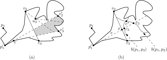
Figure 2: (a) The region (the gray region) in the subdivision with respect to $p_{1}^{\prime}$ containing $c^{*}$ is subdivided with respect to $p_{2}$. (b) $c^{*}$ is the intersection point between $b(p_{1},p_{2})$ and $b(p_{1},p_{3})$.

Assume that $c^{*}$ exists in $P$. Then it lies in the subpolygon $P^{\prime}$ of $P$ bounded by $v_{2}v_{3}$ and not containing $p_{1}$. We claim that the part of $\pi(p_{1},c^{*})$ contained in $P^{\prime}$ is just a line segment. Assume to the contrary that $\pi(p_{1},c^{*})\cap P^{\prime}$ is a chain of at least two line segments. Then each point $q$ where the chain makes a turn is a vertex of $P^{\prime}$ other than $v_{2}$ and $v_{3}$. Then $\pi(p_{2},c^{*})$ or $\pi(p_{3},c^{*})$ also passes through $q$ because $q$ is a vertex of $P$ and $\pi(p_{i},c^{*})$ do not cross each other for $i=1,2,3$. This is a contradiction. To see this, observe that $c^{*}$ is an intersection point of $b(p_{1},p_{2})$, $b(p_{2},p_{3})$ and $b(p_{3},p_{1})$. Thus, for any point $x$ in $b(p_{1},p_{2})$ (or $b(p_{3},p_{1})$), there is no vertex of $P$ where both $\pi(p_{1},x)$ and $\pi(p_{2},x)$ (or $\pi(p_{3},x)$) make a turn. Therefore, the part of $\pi(p_{1},c^{*})$ contained in $P^{\prime}$ is a line segment.

Consider the subdivision of $P^{\prime}$ by the extensions of the edges of $\pi(p_{1}^{\prime},v_{2})\cup\pi(p_{1}^{\prime},v_{3})$ with respect to $p_{1}^{\prime}$. Figure 2(a) shows a region (gray) in such a subdivision. We find the region $C$ containing $c^{*}$ by applying binary search on the extensions. For an extension $e$, we determine which side of $e$ in $P^{\prime}$ contains $c^{*}$ as follows. There is at most one point on $e$ equidistant from $p_{1}$ and $p_{i}$ for $i=2$ or $3$. Let $c_{i}$ be the intersection point of $b(p_{1},p_{i})$ with $e$. Figure 2(b) shows $b(p_{1},p_{2})$ and $b(p_{1},p_{3})$ contained in $P^{\prime}$. Each bisecting curve is a simple connected curve and it intersects $e$ at most once by the construction of $e$. Moreover, $b(p_{1},p_{i})$ intersects $\pi(p_{i},x)$ exactly once for $i=2,3$, where $x$ is the intersection point of $v_{2}v_{3}$ with $e$. And $c^{*}$ is an intersection point of $b(p_{1},p_{2})$ and $b(p_{1},p_{3})$. Therefore, if $b(p_{1},p_{i})$ does not intersect $e$, the point $c^{*}$ lies in the side of $e$ containing $v_{i}$ for $i=2,3$. If $c_{2}$ comes after $c_{3}$ along $e$ from $p_{1}^{\prime}$, the point $c^{*}$ lies in the side of $e$ containing $v_{2}$ . Otherwise, $c^{*}$ lies in the side of $e$ containing $v_{3}$. Thus we can determine which part of $e$ inside $P^{\prime}$ contains $c^{*}$ in constant time after computing $c_{2}$ and $c_{3}$ in $O(\log n)$. To compute the extension from an edge, we can use the ray-shooting algorithm which takes $O(\log n)$ time [6] since the endpoints of the extensions lie on the boundary of $P$. Therefore, we can find the region $C$ containing $c^{*}$ in the subdivision of $P^{\prime}$ with respect to $p_{1}^{\prime}$ in $O(\log^{2}n)$ time.

We let $vv_{2}^{\prime}$ and $vv_{3}^{\prime}$ be two extensions bounding $C$. See the gray region in Figure 2(a). By applying binary search on $\pi(v_{2},v_{2}^{\prime})$, we find the junction $u_{2}$ of $\pi(p_{2}^{\prime},v_{2}^{\prime})$ and $\pi(p_{2}^{\prime},c^{*})$ in $O(\log^{2}n)$ time as follows. We find the point $c_{2}^{\prime}$ on the extension of an edge on $\pi(v_{2},v_{2}^{\prime})$ that is equidistant from $p_{1}$ and $p_{2}$ in $O(\log n)$ time. Then we compare $d(c_{2}^{\prime},p_{1})$ and $d(c_{2}^{\prime},p_{3})$, which determines whether the junction $u_{2}$ lies before the edge from $p_{2}^{\prime}$ along $\pi(p_{2}^{\prime},v_{2}^{\prime})$ or not. We also do this for $p_{3}$ and find the junction $u_{3}$ of $\pi(p_{3}^{\prime},v_{3}^{\prime})$ and $\pi(p_{3}^{\prime},c^{*})$ in $O(\log^{2}n)$ time.

Now we have the junction $u_{i}$ of $\pi(p_{i},v_{i}^{\prime})$ and $\pi(p_{i},c^{*})$ for all $i=2,3$. We observe that the geodesic path $\pi(p_{i},c^{*})$ is the concatenation of $\pi(p_{i},u_{i})$ and the line segment $u_{i}c^{*}$. Therefore $d(p_{j},\cdot)$ for $j=1,2,3$ is a hyperbolic function with some domain $D$ containing $c^{*}$. We compute the three hyperbolic functions and find points where the three hyperbolic functions have the same value without considering $D$. Since we do not consider $D$, some point that we compute may not be equidistant from $p_{1},p_{2}$ and $p_{3}$. We check additionally if each such point is equidistant from the three points. In this way, we can compute $c^{*}$ in $O(\log^{2}n)$ time in total. ∎

3.1.2 The Point Equidistant from Two Points and a Line Segment

Using a way similar to the one in Section 3.1.1, we can compute the point equidistant from two points in $P$ and a line segment contained in $P$ under the geodesic metric. Given two points and a line segment contained in $P$, if more than one point of $P$ are equidistant from them, we choose the one closest to them. This will be also used as a subprocedure for computing Voronoi diagrams.

Lemma 7.

Given any two points and any line segment contained in a simple $n$-gon $P$, we can compute the closest equidistant point from them under the geodesic metric in $O(\log^{2}n)$ time if it exists.

Proof.

Let $p_{1}$ and $p_{2}$ be any two points in $P$, and $t_{1}t_{2}$ be any line segment contained in $P$. We compute two points $t_{1}^{\prime}$ and $t_{2}^{\prime}$ on $t_{1}t_{2}$ that are closest to $p_{1}$ and $p_{2}$ in $O(\log n)$ time, respectively. We compute the junction $p_{1}^{\prime}$ of $\pi(p_{1},p_{2})$ and $\pi(p_{1},t_{1}^{\prime})$, and the junction $p_{2}^{\prime}$ of $\pi(p_{2},p_{1})$ and $\pi(p_{2},t_{2}^{\prime})$ in $O(\log n)$ time. Without loss of generality, we assume that $t_{1}^{\prime},t_{2}^{\prime},p_{2}^{\prime}$ and $p_{1}^{\prime}$ appear in order along the boundary of the geodesic convex hull ch of them as shown in Figure 3. Note that the interior of ch is connected.

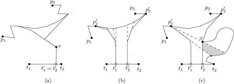
Figure 3: (a) $t_{1}^{\prime}$ may coincide with $t_{2}^{\prime}$. (b) The subdivision of ch with respect to $t_{1}^{\prime}t_{2}^{\prime}$. (c) If $c$ lies on $\pi(p_{2},t_{2}^{\prime})$, we first consider the subdivision $P^{\prime}$ with respect to $p_{1}^{\prime}$ and find the region containing $c^{*}$ (the gray region). Then consider the subdivisions of the region with respect to $t_{1}t_{2}$ and $p_{2}^{\prime}$, find the regions containing $c$, and compute $c$ directly inside their intersection.

Let $c^{*}$ be the closest equidistant point from $p_{1}$, $p_{2}$ and $t_{1}t_{2}$ in $P$. We first compute the geodesic center $c$ of them in $O(\log^{2}n)$ time as follows. If $c$ lies on the boundary of ch, we can compute it in $O(\log n)$ time since it is the midpoint of two points from $p_{1},p_{2},t_{1}^{\prime}$ and $t_{2}^{\prime}$. Thus we assume that $c$ lies in the interior of ch.

Consider the subdivision of ch with respect to $p_{1}^{\prime}$ by the extensions of edges in $\pi(p_{1}^{\prime},t_{1}^{\prime})\cup\pi(p_{1}^{\prime},p_{2}^{\prime})$ in direction opposite to $p_{1}^{\prime}$. We can determine which side of a given extension contains $c$ in $O(\log n)$ time. Therefore, we can compute the region of the subdivision containing $c$ in $O(\log^{2}n)$ time without constructing the subdivision as we do for the first level binary search in Section 3.1. Similarly, we can compute the region of the subdivision of ch containing $c$ with respect to $p_{2}^{\prime}$ by the extensions of edges in $\pi(p_{2}^{\prime},t_{2}^{\prime})\cup\pi(p_{2}^{\prime},p_{1}^{\prime})$ in direction opposite to $p_{2}^{\prime}$ in the same time. Now consider the subdivision of ch by the extensions of edges in $\pi(t_{1}^{\prime},p_{1}^{\prime})\cup\pi(t_{2}^{\prime},p_{2}^{\prime})$ in direction opposite to $t_{1}^{\prime}$ and $t_{2}^{\prime}$. See Figure 3(b). We can compute the region of the subdivision containing $c$ in the same time. Then the intersection of the three regions is a convex polygon with at most six vertices and we can find the geodesic center $c$ in the intersection in constant time.

If $c$ is equidistant from $p_{1}$, $p_{2}$ and $t_{1}t_{2}$, we are done. Otherwise, it is equidistant from only two of them and it lies in the shortest path connecting the two in $P$. Let $xy$ be the edge of the shortest path that contains $c$. If $xy$ is not on the boundary of the interior of ch, then $P$ has no point equidistant from $p_{1}$, $p_{2}$ and $t_{1}t_{2}$ by an argument similar to the one in the first paragraph of the proof of Lemma 6.

Assume that $xy$ is on the boundary of the interior of ch. Then $xy$ subdivides $P$ into two subpolygons and $c^{*}$, if it exists in $P$, lies in the subpolygon $P^{\prime}$ not containing the interior of ch. In the case that $xy$ lies on $\pi(p_{1},p_{2})$, consider the subdivision of $P^{\prime}$ with respect to $t_{1}^{\prime}t_{2}^{\prime}$ by the extensions of edges in $\pi(t_{1}^{\prime},x)\cup\pi(t_{2}^{\prime},y)$ towards $P^{\prime}$. For the other case, that is, $xy$ lies on $\pi(p_{i},t_{i}^{\prime})$ for $i=1$ or $2$, consider the subdivision of $P^{\prime}$ with respect to $p_{j}^{\prime}$ by the extension of edges in $\pi(p_{j}^{\prime},x)\cup\pi(p_{j}^{\prime},y)$ for $j\in\{1,2\}\setminus\{i\}$. For an extension $e$, we determine which side of $e$ in $P^{\prime}$ contains $c^{*}$ as follows. We compute the intersection point $q$ of $b(p_{1},p_{2})$ with $e$ by performing binary search on the intersections of $e$ by the extensions of edges on the shortest path from $p_{2}$ to an endpoint of $e$. Then we determine which side of $e$ contains $c$ by comparing the geodesic distances $d(p_{1},q)$ and $d(t_{1}t_{2},q)$. This can be done in $O(\log n)$ time as the intersection point $q$ and the distances can be computed in $O(\log n)$ time. See Figure 3(c). In any case, as we do in the proof of Lemma 6, we can find $c^{*}$ in $P^{\prime}$ in $O(\log^{2}n)$ time if it exists. ∎

3.2 The Geodesic Center of Points in a Simple Polygon

Combining the result in the previous subsection with the algorithms for computing the center of points in the plane [13] and for computing the geodesic center of a simple polygon [17], we can compute the geodesic center of a set of $m$ points contained in a simple polygon $P$ with $n$ vertices in $O(m\log m\log^{2}n)$ time after computing the shortest path data structure for $P$. This algorithm will be used as a subprocedure for computing the topological structure of the geodesic farthest-point Voronoi diagram of points in $P$.

To compute the center of a simple polygon, Pollack et al. [17] first triangulate the input polygon and construct a balanced binary search tree on the chords of the triangulation using the algorithm by Guibas et al [8]. Then, they find the triangle $t$ of the triangulation containing the geodesic center by applying binary search with a chord-oracle to the balanced binary search tree. A chord-oracle is the procedure for determining which side of a given chord contains the geodesic center. They subdivide $t$ further and locate a smaller triangle $t^{\prime}$ such that the geodesic path from a vertex of $P$ to any point in $t^{\prime}$ has the same combinatorial structure. Finally, they find the center inside $t^{\prime}$ which is the lowest point of the upper envelope of some distance functions within domain $t^{\prime}$.

To remove the linear dependency of $n$ in the time complexity of our algorithm, we again use the shortest path data structure. We may assume that we already have the triangulation of $P$ and the balanced binary search tree on the chords because the algorithm for constructing the shortest path data structure constructs them.

Computing the triangle of the triangulation containing the geodesic center.

Let $c$ be the geodesic center of $S$. We apply a chord-oracle described in Lemma 8 to $O(\log n)$ chords of the triangulation and find the triangle $t$ containing $c$ in $O(m\log^{2}n)$ time.

Lemma 8.

Given a chord of $P$, we can determine which side of the chord contains the geodesic center in $O(m\log n)$ time.

Proof.

Let $e$ be a given chord. We will find the point $c_{e}$ on $e$ that minimizes the geodesic distance from its farthest site in $S$. Based on $c_{e}$ and its farthest sites in $S$, we can determine which side of $e$ contains $c$ in constant time using the method by Pollack et al [17].

To compute $c_{e}$, we do the followings. The chord subdivides $P$ into two regions. Let $S_{1}$ be the set of sites in $S$ contained in one region of $P$ and $S_{2}$ be the set of sites in $S$ contained in the other region of $P$. We pair the sites in the same set $S_{i}$ for $i=1,2$. Then we have $\lfloor m/2\rfloor+1$ pairs. For any pair $(s,s^{\prime})$ we have, the bisecting curve of $s$ and $s^{\prime}$ intersects $e$ at most once because both $s$ and $s^{\prime}$ lie in the same side of $e$. We can prune and search on $S$ with this property.

We compute the intersection $p$ of the bisecting curve of $s$ and $s^{\prime}$ with $e$ for each pair $(s,s^{\prime})$ in $O(\log n)$ time as follows. Observe that $e$ is subdivided into $O(n)$ disjoint line segments by the extensions with respect to $s$ and by the extensions with respect to $s^{\prime}$. We observe that $p$ lies between $x$ and $x^{\prime}$, where $x$ and $x^{\prime}$ are the points on $e$ that are closest to $s$ and $s^{\prime}$, respectively. We can compute $x$ and $x^{\prime}$ in $O(\log n)$ time. We apply binary search on the line segments in the subdivision lying between $x$ and $x^{\prime}$ to find $p$ as follows. Initially, the search space for $s$ is the set of the extensions of edges of $\pi(s,x)\cup\pi(s,x^{\prime})$ towards $xx^{\prime}$, and the search space for $s^{\prime}$ is the set of the extensions of edges of $\pi(s^{\prime},x)\cup\pi(s^{\prime},x^{\prime})$ towards $xx^{\prime}$. For each iteration of the binary search, we choose the median of each search space, and let $q$ and $q^{\prime}$ be the intersection of $xx^{\prime}$ with the two medians. We can choose one line segment which does not contain $p$ among $xq$, $xq^{\prime}$, $x^{\prime}q$ and $x^{\prime}q^{\prime}$ in constant time based on distances $d(s,q)$ and $d(s^{\prime},q^{\prime})$. This is because one of $d(s,\cdot)$ and $d(s^{\prime},\cdot)$ is increasing and the other is decreasing in the domain of $xx^{\prime}$. Since at least one of the two search spaces is reduced by a constant fraction in every iteration, we can find $p$ in $O(\log n)$ time.

We find the median of the $\lfloor m/2\rfloor+1$ intersections by the bisecting curves on $e$ and determine which side of the median contains $c_{e}$ in $m\cdot O(\log n)$ time using the convexity of $d(s,\cdot)$ on $e$ for each site $s$ in $S$. Let $e^{\prime}$ be the side (line segment) of the median in $e$ that does not contain $c_{e}$. There are at least $\lfloor m/4\rfloor$ pairs of sites whose intersection points lie on $e^{\prime}$. For such a pair $(s,s^{\prime})$, we have either $d(s,z)>d(s^{\prime},z)$ or $d(s,z)<d(s^{\prime},z)$ for every point $z\in e\setminus e^{\prime}$. Thus we can discard at least one site for each such pair: discard $s$ if $d(s,z)<d(s^{\prime},z)$, and discard $s^{\prime}$ otherwise. Therefore, we can discard at least $\lfloor m/4\rfloor$ sites in each iteration.

After discarding at least $\lfloor m/4\rfloor$ sites, we update $S_{1}$ and $S_{2}$ accordingly. Then we pair the remaining sites in the same set and discard some sites repeatedly until there remain only a constant number of candidates of the sites in $S$ farthest from $c_{e}$. This takes $O(m\log n)$ time because the number of sites in $S$ we consider decreases by a constant factor.

For a constant number of candidates, we compute $c_{e}$ directly in $O(\log n)$ time as we do in Section 3.1. ∎

Finding a small triangle containing the geodesic center.

Now we have the triangle $t$ of the triangulation containing $c$. For each site $s$, we consider the geodesic convex hull $\textsc{ch}_{s}$ of $s\cup t$. Imagine the subdivision of $t$ by the extensions of the edges of $\textsc{ch}_{s}$, except the edges of $t$, towards $t$. See Figure 4(a). Every region in this subdivision is a convex polygon with at most five vertices. These regions can be sorted along the boundary of $t$.

Applying binary search, we can find the region in the subdivision of $t$ with respect to $s$ containing $c$ in $O(m\log^{2}n)$ time. However, in this case, we have $m$ sites. If we do this for every site, it takes $O(m^{2}\log^{2}n)$ time. To do this more efficiently, we apply additional prune and search.

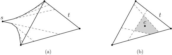
Figure 4: (a) The subdivision of $t$ with respect to a site $s$. (b) The arrangement of extensions from the subdivisions of $t$ with respect to the sites in $S$.

For each site $s$, we choose the median extension in the subdivision of $t$ with respect to $s$. Let $L$ be the set of all median extensions from all sites. See Figure 4(b). For a site $s$, the search space (regions in the subdivision of $t$ with respect to $s$) can be halved by determining which side of the median extension for $s$ in $L$ contains $c$. Once we have the region containing $c$ in the arrangement of $L$, we can determine which side of the median extension for $s$ for every site $s$. We find the region containing $c$ in the arrangement of $L$ using a $(1/r)$-cutting for $L$ as follows.

Consider the range space

$$X=(L,\{\{\ell\in L:\ell\cap\tau\neq\phi\}:\tau\subseteq t\textnormal{ is a triangle.}\}).$$

Then $X$ has finite VC-dimension, which can be shown by using a way similar to the one for lines in the plane [5]. Let $r$ be a sufficiently large constant. We compute an $(1/r)$-net $N\subseteq L$ for $X$ of size $O(r\log r)$. Then any triangle in the triangulation of $N$ intersects $O(|L|/r)$ line segments by the property of $(1/r)$-nets, where $|L|$ denotes the cardinality of $L$. Note that every line segment in $N$ is a chord of $P$. By applying the chord-oracle for every line segment in $N$, we can compute the triangle $t^{\prime}$ in the triangulation of $N$ containing $c$ in $O(m\log n)$ time. We search further with the line segments in $L$ intersecting $t^{\prime}$. In $O(\log m)$ iterations, we can find a triangle $\tau\subseteq t^{\prime}$ containing $c$ which is intersected by a constant number of line segments in $L$. Then we directly compute the region of the arrangement of $L$ containing $c$ in $O(\log n)$ time. This takes $O(m\log m\log n)$ time in total.

Therefore, in $O(m\log m\log n)$ time, the search space is halved (regions in the subdivision of $t$) for every site $s$. Thus, in $O(m\log m\log^{2}n)$ time, we can find the region containing $c$ in the subdivision of $t$ with respect to $s$ for every site $s$.

We can compute the intersection of all the regions containing $c$ in $O(m\log m)$ time because each region is a convex polygon with at most five vertices. After computing the intersection, we triangulate the intersection and find the triangle containing $c$ in $O(m\log m\log n)$ time. The resulting triangle $\tau^{\prime}$ satisfies the condition we want to obtain.

Finding the geodesic center inside the smaller triangle.

For each site $s$, the geodesic path $\pi(s,x)$ between $s$ and any point $x$ in $\tau^{\prime}$ has the same combinatorial structure, which means that $\pi(s,x)$ is a hyperbolic function. Thus, our problem reduces to computing the lowest point of the upper envelope of $O(m)$ functions. Pollack et al. [17] present a procedure for this problem that takes $O(m)$ time.

Therefore, we have the following theorem.

Theorem 9.

The geodesic center of $m$ points contained in a simple polygon with $n$ vertices can be computed in $O(m\log m\log^{2}n)$ time after the shortest path data structure for the simple polygon is constructed.

4 Topological Structures of Voronoi Diagrams

In this section, we define the topological structure of a Voronoi diagram and show how to compute the Voronoi diagram from its topological structure. The topological structure of a Voronoi diagram represents the adjacency of the Voronoi cells.

The common boundary of any two adjacent Voronoi cells is connected for the nearest-point and farthest-point Voronoi diagrams of point sites in a simple polygon [2, 3]. Similarly, this also holds for the higher-order Voronoi diagram of point sites in a simple polygon.

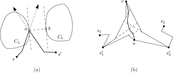
Figure 5: (a) For any point $x$ in $\pi(a,b)$, we have $d(x,s)\geq d(x,s^{\prime})$. This contradicts that $C_{a}$ and $C_{b}$ are in the same Voronoi cell of $k\textnormal{-}\textsf{VD}$. (b) The number of edges in the common boundary of two adjacent Voronoi cells is bounded by the total complexity of $\pi(s_{1}^{\prime},v)$, $\pi(s_{1}^{\prime},u)$, $\pi(s_{2}^{\prime},v)$ and $\pi(s_{2}^{\prime},u)$, where $u$ and $v$ are endpoints of the common boundary.

Lemma 10.

A Voronoi cell of $k\textnormal{-}\textsf{VD}$ is connected for any $k$ with $1\leq k\leq m-1$. Moreover, the common boundary of any two adjacent Voronoi cells in $k\textnormal{-}\textsf{VD}$ is connected.

Proof.

Assume to the contrary that the Voronoi cell of a $k$-tuple is not connected. Consider two connected components $C_{a}$ and $C_{b}$ of the Voronoi cell, and let $a$ and $b$ be the two points with $a\in C_{a}$ and $b\in C_{b}$ that minimize $d(a,b)$. Note that the line tangent to $C_{a}$ at $a$ is orthogonal to the edge of $\pi(a,b)$ incident to $a$. See Figure 5(a). Since $a$ is on the boundary of the Voronoi cell, it lies on the bisecting curve of two sites, say $s$ and $s^{\prime}$. We claim that $C_{a}$ and $C_{b}$ lie in different sides of $b(s,s^{\prime})$, which contradicts that $C_{a}$ and $C_{b}$ are contained in the same Voronoi cell of $k\textnormal{-}\textsf{VD}$. For any point $x$ in $\pi(a,s)$, we have $d(x,s)\leq d(x,s^{\prime})$. Similarly, for any point $x$ in $\pi(a,s^{\prime})$, we have $d(x,s)\geq d(x,s^{\prime})$. Also, consider the extension of the edge of $\pi(a,s)$ incident to $a$ towards $a$ until it reaches the boundary of $P$. For any point $x$ in this extension, we have $d(x,s)\geq d(x,s^{\prime})$. Similarly, we have $d(x,s)\leq d(x,s^{\prime})$ for any point $x$ on the extension of the edge of $\pi(a,s^{\prime})$ incident to $a$ towards $a$ until it reaches the boundary of $P$. This implies that for any point $x$ in $\pi(a,b)$, we have $d(x,s)\geq d(x,s^{\prime})$. Therefore the claim holds.

For the second part of the lemma, observe that the common boundary of the Voronoi cells of any two distinct $k$-tuples $S_{k}$ and $S_{k}^{\prime}$ of $S$ is a part of the bisecting curve of two sites $s$ and $s^{\prime}$ with $s\in S_{k}\setminus S_{k}^{\prime}$ and $s^{\prime}\in S_{k}^{\prime}\setminus S_{k}$. Let $p$ be an endpoint of a connected component $\Gamma$ of the common boundary. We show that $b(s,s^{\prime})\setminus\Gamma$ is not contained in the common boundary. Note that $p$ is a degree-3 vertex of $k\textnormal{-}\textsf{VD}$, which is equidistant from $s,s^{\prime}$ and another site, say $s^{\prime\prime}$. Consider the nearest-point Voronoi diagram of $s,s^{\prime}$ and $s^{\prime\prime}$. Since the common boundary of any two Voronoi cells is connected for this diagram [2], we have $d(s^{\prime\prime},x)<d(s,x)=d(s^{\prime},x)$ for any point $x$ lying on the connected component of $b(s,s^{\prime})\setminus\Gamma$ with endpoint $p$. Therefore, the connected component of $b(s,s^{\prime})\setminus\Gamma$ with endpoint $p$ is not contained in the common boundary. Similarly, we can prove that the other component of $b(s,s^{\prime})\setminus\Gamma$ is not contained in the common boundary, and thus the lemma holds. ∎

The topological structure of $k\textnormal{-}\textsf{VD}$ is defined as follows for $1\leq k\leq m-1$. Imagine that we apply vertex suppression for every degree-2 vertex of the Voronoi diagram while preserving the topology of the Voronoi diagram. Vertex suppression of a vertex $v$ of degree 2 is the operation of removing $v$ (and the edges incident to $v$) and adding an edge connecting the two neighboring vertices of $v$. Then the resulting graph consists of vertices of degree-1 and degree-3 and edges connecting the vertices. We call the dual of the resulting graph the adjacency graph of the Voronoi diagram. The adjacency graph is a planar graph with complexity $O(k(m-k))$, because the number of degree-1 and degree-3 vertices of $k\textnormal{-}\textsf{VD}$ is $O(k(m-k))$ [12]. The adjacency graph of a Voronoi diagram represents the topological structure of the Voronoi diagram.

Assume that we have the adjacency graph of the Voronoi diagram together with the exact positions of the degree-1 and degree-3 vertices of the Voronoi diagram. Each Voronoi cell is defined by $k$ sites, but any two adjacent Voronoi cells share $k-1$ sites. Consider two adjacent Voronoi cells $V_{1}$ and $V_{2}$. Let $s_{1}$ and $s_{2}$ be the two sites defining $V_{1}$ and $V_{2}$, respectively, which are not shared by them. Then the common boundary of $V_{1}$ and $V_{2}$ is a simple curve connecting two Voronoi vertices $v$ and $u$ of degree-1 or degree-3 such that each Voronoi edge in the common boundary is a part of $b(s_{1},s_{2})$ lying between $v$ and $u$. See Figure 5(b).

To compute the Voronoi edges in the common boundary of $V_{1}$ and $V_{2}$, we consider the geodesic paths $\pi(s_{i}^{\prime},v)$ and $\pi(s_{i}^{\prime},u)$ for $i=1,2$, where $s_{i}^{\prime}$ is the junction of $\pi(s_{i},v)$ and $\pi(s_{i},u)$. Then for any vertex $x$ in $\pi(s_{1}^{\prime},v)\cup\pi(s_{1}^{\prime},u)$, there exists a point $q$ in $b(s_{1},s_{2})$ lying between $v$ and $u$ such that $\pi(s_{1},q)$ and $\pi(s_{1},x)$ have the same combinatorial structure. The same holds for $s_{2}$. This implies that the number of edges in the common boundary is bounded by the total complexity of $\pi(s_{1}^{\prime},v)\cup\pi(s_{1}^{\prime},u)$ and $\pi(s_{2}^{\prime},v)\cup\pi(s_{2}^{\prime},u)$. Thus, we compute the geodesic paths explicitly and consider every edge of the geodesic paths.

Therefore, we can compute the common boundary of two adjacent Voronoi cells in time linear to its complexity plus $O(\log n)$. This leads to $O(T_{1}+T_{2}\log n)$ time for computing the Voronoi diagram from the topological structure of the diagram, where $T_{1}$ is the combinatorial complexity of the Voronoi diagram and $T_{2}$ is the combinatorial complexity of the adjacency graph.

Lemma 11.

We can compute the Voronoi diagram of $m$ points in a simple polygon with $n$ vertices in $O(T_{1}+T_{2}\log n)$ time once the adjacency graph and the exact positions of the degree-1 and degree-3 vertices of the Voronoi diagram are given, where $T_{1}$ is the combinatorial complexity of the Voronoi diagram and $T_{2}$ is the combinatorial complexity of the adjacency graph.

Therefore, in the following, we focus on computing the adjacency graphs and the exact positions of the degree-1 and degree-3 vertices of VD, $k\textnormal{-}\textsf{VD}$ and FVD.

5 The Geodesic Nearest-Point Voronoi Diagram

Fortune [7] presented an $O(m\log m)$-time algorithm to compute the nearest-point Voronoi diagram of $m$ points in the plane by sweeping the plane with a horizontal line from top to bottom. During the sweep, the algorithm computes a part of the Voronoi diagram of sites lying above the horizontal line, which finally becomes the complete Voronoi diagram in the end of the sweep. Fortune defined two types of events and showed how the algorithm processes $O(m)$ events in the order of their $y$-coordinates to compute the Voronoi diagram. Each event can be handled in $O(\log m)$ time, which leads to $O(m\log m)$ total running time.

In our case, we sweep the polygon with a geodesic path $\pi(o,x)$ for a fixed point $o$ on the boundary of $P$ and a point $x$ moving along the boundary of $P$ from $o$ in clockwise order. The point $x$ is called the sweep point. If we compute all degree-1, degree-2 and degree-3 vertices of the Voronoi diagram during the sweep, we may not achieve the running time better than $O((n+m)\log(n+m))$ as there are $O(n+m)$ such vertices. The key to improve the running time is to compute the topological structure of the Voronoi diagram first which consists of the degree-1 and degree-3 vertices of the Voronoi diagram and the adjacency of the Voronoi cells. Then we construct the complete Voronoi diagram, including degree-2 vertices, from its topological structure using Lemma 11.

Let $o$ be an arbitrary point on $\partial P$, where $\partial P$ denotes the boundary of $P$. Consider the sweep point $x$ that moves from $o$ along $\partial P$ in clockwise order. We use $P(x)$ to denote the subpolygon of $P$ bounded by $\pi(o,x)$ and the part of $\partial P$ from $o$ to $x$ in clockwise order. In other words, $P(x)$ is the region swept by $\pi(o,x)$. Note that $P(x)$ is weakly simple. See Figure 6. Clearly, $P(x_{1})\subseteq P(x_{2})$ for any two points $x_{1}$ and $x_{2}$ on $\partial P$ such that $x_{1}$ comes before $x_{2}$ from $o$ in clockwise order along $\partial P$.

For a site $s\in P(x)$, let $R_{s}(x)$ be the set $\{p\in P(x)\mid d(p,s)\leq d(p,\pi(o,x))\}$. By definition, $R_{s}(x_{1})\subseteq R_{s}(x_{2})$ for any two points $x_{1}$ and $x_{2}$ on $\partial P$ such that $x_{1}$ comes before $x_{2}$ from $o$ in clockwise order along $\partial P$.

Lemma 12.

If $s$ lies on an edge of $\pi(o,x)$, $R_{s}(x)$ is a line segment that is incident to $s$ and orthogonal to the edge.

Proof.

Let $\gamma_{s}$ be the boundary of $R_{s}(x)$. By definition, $d(p,s)=d(p,\pi(o,x))$ for any point $p$ in $\gamma_{s}$. Note that $d(p,s)=d(p,\pi(o,x))$ if and only if $s$ is the point of $\pi(o,x)$ closest to $p$ under the geodesic metric. This is because $s$ lies on $\pi(o,x)$. Therefore, for any point $p$ in $\gamma_{s}$, the edge of $\pi(s,p)$ incident to $s$ is orthogonal to the edge of $\pi(o,x)$ containing $s$.

Moreover, we claim that $\gamma_{s}$ consists of a single line segment. If $\pi(p,s)$ consists of more than one line segment for some point $p$ on $\gamma_{s}$, we can choose a sufficiently small neighborhood $N_{p}$ of $p$ contained in $P^{\prime}$ such that the point on $\pi(o,x)$ closest to $p^{\prime}$ is $s$ for any point $p^{\prime}\in N_{p}$. This implies that $N_{p}$ is contained in $R(x)$, which contradicts that $\gamma_{s}$ is a part of the boundary of $R(x)$. ∎

Lemma 13.

For a site $s\in P(x)$, $R_{s}(x)$ is connected.

Proof.

If $s\in\pi(o,x)$, $R_{s}(x)$ is a line segment by Lemma 12, and therefore it is connected. In the following, we assume that $s$ is not on $\pi(o,x)$ and show that $\pi(p,s)\subseteq R_{s}(x)$ for any point $p\in R_{s}(x)$. This implies that $R_{s}(x)$ is connected because $s$ is contained in $R_{s}(x)$ if $s\in P(x)$ by definition. Let $p$ be a point in $R_{s}(x)$. Consider a point $r\in\pi(p,s)$. We have $d(r,s)=d(p,s)-d(p,r)$. Moreover, we have $d(p,\pi(o,x))-d(p,r)\leq d(r,\pi(o,x))$. Since $p\in R_{s}(x)$, it holds that $d(p,s)\leq d(p,\pi(o,x))$. Thus, $d(r,s)\leq d(r,\pi(o,x))$, and $r$ is also in $R_{s}(x)$ by definition. Therefore $R_{s}(x)$ is connected. ∎

We say that a subset $A$ of $P$ is weakly monotone with respect to a geodesic path $\gamma$ if the intersection of $\pi(p,\gamma)$ with $A$ is connected for any point $p\in A$. We define a shaft from a point $x\in P$ towards a direction to be the line segment connecting $x$ and $y$, where $y$ is the first intersection point of the boundary of $P$ with the ray from $x$ towards the direction.

Lemma 14.

For a site $s\in P(x)\setminus\pi(o,x)$, the boundary of $R_{s}(x)$ consists of one polygonal chain of $\partial P(x)$ and a simple curve whose both endpoints lie on $\partial P(x)$. Moreover, the simple curve is weakly monotone with respect to $\pi(o,x)$.

Proof.

By Lemma 13, $R_{s}(x)$ is connected. Thus to prove the first part of the lemma, it suffices to show that the boundary of $R_{s}(x)$ intersects $\partial P(x)$. To do this, consider the shaft from a point $p\in R_{s}(x)$ in direction opposite to the edge of $\pi(p,\pi(o,x))$ incident to $p$. We claim that the shaft is contained in $R_{s}(x)$. This is because $d(r,\pi(o,x))=d(p,\pi(o,x))+d(p,r)\geq d(p,s)+d(p,r)\geq d(r,s)$ for any point $r$ in the shaft by triangle inequality and the fact that $R_{s}(x)$ contains no point of $\pi(o,x)$. Note that an endpoint of the shaft is on $\partial P(x)$. Therefore, $R_{s}(x)$ intersects $\partial P(x)$, and the first part of the lemma holds.

For the second part of the lemma, we claim that $\pi(p,\pi(o,x))\setminus\{p\}$ does not intersect $R_{s}(x)$ for any point $p$ on $\partial R_{s}(x)\setminus\partial P(x)$. Assume to the contrary that a point $p^{\prime}$ in the path is in $R_{s}(x)$. We already showed that the shaft from $p^{\prime}$ in direction opposite to the edge of $\pi(p^{\prime},\pi(o,x))$ incident to $p^{\prime}$ is contained in $R_{s}(x)$. Note that the shaft contains $p$. This contradicts that $p$ lies on the boundary of $R_{s}(x)$. Therefore, the second part of the lemma also holds. ∎

Now we consider the union of $R_{s}(x)$ for every site $s$ in $P(x)$ and denote it by $R(x)$. Figure 6 shows three sites contained in $P(x)$ for a simple polygon $P$. The dashed region in Figure 6(a) is $R(x)$. Note that for any point $p\in P(x)$ and any site $s$ lying outside of $P(x)$, it holds that $d(p,\pi(o,x))<d(p,s)$. This implies that for any point $p\in R(x)$, the nearest site of $p$ is in $P(x)$. Therefore, for computing VD restricted to $R(x)$, we do not need to consider any sites lying outside of $P(x)$.

The following corollaries follow from the properties of $R_{s}(x)$.

Corollary 15.

The closure of $P(x)\setminus R(x)$ is weakly simple.

Corollary 16.

Each connected component of $R(x)$ consists of a polygonal chain of $\partial P$ and a simple curve with endpoints on $\partial P$ unless $\pi(o,x)$ contains a site. Moreover, the union of such curves is weakly monotone with respect to $\pi(o,x)$ at any time.

We maintain the geodesic nearest-point Voronoi diagram restricted to $R(x)$ of the sites contained in $P(x)$ while $x$ moves along $\partial P$. However, after the sweep, $R(x)$ is still a proper subpolygon $P$, and therefore VD is not completed yet. To resolve this, we attach a long and very thin triangle to $P$ to make a bit larger simple polygon $P^{\prime}$ and set $o$ to lie at the tip of the triangle, as illustrated in Figure 6, so that once we finish the sweep (when the sweep point returns back to $o$) in $P^{\prime}$ we have the complete Voronoi diagram in $P$. (The triangle has height of the diameter of $P$.)

The beach line and the breakpoints.

There are $O(m)$ connected components of $R(x)$ each of whose boundary consists of a polygonal chain of $\partial P$ and a connected simple curve. The beach line is defined to be the union of the $O(m)$ simple curves of $R(x)$. The beach line has properties similar to those of the beach line of the Euclidean Voronoi diagram. It consists of $O(n+m)$ hyperbolic or linear arcs. We do not maintain them explicitly because the complexity of the sequence is too large for our purpose. Instead, we maintain the combinatorial structure of the beach line using $O(m)$ space as follows.

A point on the beach line is called a breakpoint if it is equidistant from two distinct sites. Each breakpoint moves and traces out a Voronoi edge as the sweep point moves along $\partial P^{\prime}$. We represent each breakpoint symbolically. That is, a breakpoint is represented as the pair of sites equidistant from it. We say that such a pair defines the breakpoint. Given the pair defining a breakpoint and the position of the sweep point, we can find the exact position of the breakpoint using Lemma 7 in $O(\log^{2}n)$ time.

Additionally, we consider the endpoints of the $O(m)$ simple curves comprising the beach line. We simply call them the endpoints of the beach line. For an endpoint $p$ of the beach line, there is a unique site $s$ satisfying $d(p,s)=d(p,\pi(o,x))$. We say that $s$ defines $p$.

By Corollary 15 and Corollary 16, we can define the order of these breakpoints and these endpoints. Let $B(x)=\langle\beta_{1},\ldots,\beta_{m^{\prime}}\rangle$ be the sequence of the breakpoints and the endpoints of the beach line sorted in clockwise order along the boundary of $P(x)\setminus R(x)$ with $m^{\prime}=O(m)$. We maintain $B(x)$ instead of the arcs on the beach line. As $x$ moves along $\partial P^{\prime}$, the sequence $B(x)$ changes. We will see that the length of $B(x)$ is $O(m)$ at any time during the move of the sweep point along $\partial P^{\prime}$.

While maintaining $B(x)$, we compute the adjacency graph of VD together with the degree-1 and degree-3 vertices of VD restricted to $R(x)$. Specifically, when a new breakpoint defined by a pair $(s,s^{\prime})$ of sites is added to $B(x)$, we add an edge connecting the node for $s$ and the node for $s^{\prime}$ into the adjacency graph.

Events.

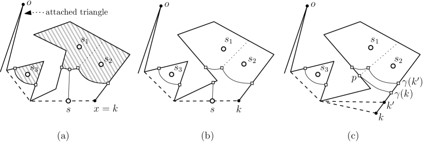
Figure 6: (a) The site event defined by $s$ with key $k$. Two (degenerate) breakpoints appear in $B(k)$. (b) Two (degenerate) endpoints appear in $B(k)$. (c) The vanishing event defined by the breakpoint of $(s_{1},s_{2})$ with key $k$. The endpoint defined by $s_{1}$ and the breakpoint merge into the endpoint defined by $s_{2}$.

We have four types of events: site events, circle events, vanishing events, and merging events. Every event corresponds to a key, which is a point on the boundary of $P^{\prime}$. We maintain the events with respect to their keys sorted in clockwise order from $o$ along the boundary. The event occurs when the sweep point $x$ passes through the corresponding key. The sequence $B(x)$ changes only when $x$ passes through the key of an event. Given a sorted sequence of $\nu$ events for $\nu\in\mathbb{N}$, we can insert a new event in $O(\log\nu)$ time since we are given each point on the boundary of $P^{\prime}$ together with the edge of $P^{\prime}$ where it lies. We can delete an event from $\nu$ in $O(\log|\nu|)$ time, and find the first event in $\nu$ and delete it in $O(1)$ time.

The definitions of the first two event types are similar to the ones in Fortune’s algorithm [7]. Each site $s$ in $S$ defines a site event. The key $k$ of the site event defined by $s$ is the point on $\partial P^{\prime}$ that comes first from $o$ in clockwise order along $\partial P^{\prime}$ among the points $x^{\prime}$ with $s\in\pi(o,x^{\prime})$. When the sweep point passes through $k$, the site $s$ appears on the beach line. At the same time, new breakpoints defined by $s$ and some other site $s^{\prime}$, or new endpoints defined by $s$ appear on $B(x)$. See Figure 6(a) and (b).

An event of the other three event types is defined by a pair of consecutive points in $B(x)$ or a single breakpoint in $B(x)$. An event is said to be valid if the two points defining the event are consecutive, or the breakpoint defining the event is in $B(\cdot)$. Before the sweep point reaches the key of an event, the two points defining the event may become non-consecutive, or the breakpoint defining the event may disappear from $B(x)$ due to the changes of $B(\cdot)$. In this case, we say that the event become invalid.

A pair $(\beta_{1},\beta_{2})$ of consecutive breakpoints in $B(x)$ defines a circle event if there is a point $c$ equidistant from $s_{1},s_{2}$ and $s_{3}$ under the geodesic metric, where $(s_{1},s_{2})$ and $(s_{2},s_{3})$ are two pairs of sites defining $\beta_{1}$ and $\beta_{2}$, respectively. The key $k$ of this circle event is the point on $\partial P^{\prime}$ that comes first from $o$ in clockwise order along $\partial P^{\prime}$ among the points $x^{\prime}$ with $d(c,\pi(o,x^{\prime}))=d(c,s_{1})(=d(c,s_{2})=d(c,s_{3}))$. If this event is valid when $x$ passes through $k$, $c$ appears on the beach line at the time. Moreover, $\beta_{1}$ and $\beta_{2}$ disappear from the beach line, and a new breakpoint defined by $(s_{1},s_{3})$ appears on the beach line. (One may regard this as merging $\beta_{1}$ and $\beta_{2}$ into the breakpoint defined by $(s_{1},s_{3})$.)

Each breakpoint $\beta$ in $B(x)$ defines a vanishing event. Let $(s_{1},s_{2})$ be the pair of sites defining $\beta$. Consider the two points on $\partial P^{\prime}$ equidistant from $s_{1}$ and $s_{2}$. We observe that exactly one of them lies outside of $R(x)$. We denote it by $p$. See Figure 6(c). The key $k$ of the vanishing event is the point on $\partial P^{\prime}$ that comes first from $o$ in clockwise order along $\partial P^{\prime}$ among the points $x^{\prime}$ with $d(p,\pi(o,x^{\prime}))=d(p,s_{1})$. Assume that this event is valid when $x$ passes through $k$. Then, $\beta$ traces out a Voronoi edge and reaches $p$, which is a degree-1 Voronoi vertex. Moreover, $B(x)$ changes accordingly as follows. Right before $x$ reaches $k$, an endpoint defined by $s_{1}$ or $s_{2}$ is a neighbor of $\beta$ in $B(x)$. (Otherwise, the beach line is not weakly monotone.) Without loss of generality, we assume that an endpoint defined by $s_{1}$ is a neighbor of $\beta$. When $x$ reaches the key, this endpoint and $\beta$ disappear from $B(x)$, and an endpoint defined by $s_{2}$ appears in $B(x)$. (One may regard this as merging the endpoint defined by $s_{1}$ and $\beta$ into the endpoint defined by $s_{2}$.)

A pair $(\beta_{1},\beta_{2})$ of consecutive endpoints in $B(x)$ defines a merging event if $\beta_{1}$ and $\beta_{2}$ are endpoints of two distinct connected curves of the beach line. Let $s_{1}$ and $s_{2}$ be the sites defining $\beta_{1}$ and $\beta_{2}$, respectively. Without loss of generality, assume that $\beta_{1}$ comes before $\beta_{2}$ from $o$ in clockwise order along $\partial P^{\prime}$. Let $p$ be the (unique) point on $\partial P^{\prime}$ equidistant from $s_{1},s_{2}$ that comes after $\beta_{1}$ and before $\beta_{2}$ from $o$ in clockwise order along $\partial P^{\prime}$. The key $k$ of the merging event is the point on $\partial P^{\prime}$ that comes first from $o$ in clockwise order along $\partial P^{\prime}$ among the points $x^{\prime}$ with $d(p,\pi(o,x^{\prime}))=d(p,s_{1})$. Assume that this event is valid when $x$ passes through $k$. Then, as the sweep point $x$ moves along $\partial P^{\prime}$, $\beta_{1}$ and $\beta_{2}$ become closer and finally meet each other at $p$. This means that the two connected curves, one containing $\beta_{1}$ and the other containing $\beta_{2}$, merge into one connected curve. At this time, $\beta_{1}$ and $\beta_{2}$ merge into a breakpoint defined by $(s_{1},s_{2})$.

5.1 An Algorithm

Initially, $B(x)=B(o)$ is empty, so there is no circle, vanishing, or merging event. We compute the keys of all site events in advance. For each site, we compute the key corresponding to its event in $O(\log n)$ time [8]. As $B(x)$ changes, we obtain new pairs of consecutive breakpoints or endpoints, and new breakpoints. Then we compute the key of each event in $O(\log^{2}n)$ time using the following lemmas and Lemma 6. In addition, as $B(x)$ changes, some event becomes invalid. Once an event becomes invalid, it does not become valid again. Thus we discard an event if it becomes invalid. Therefore, the number of events we have is $O(|B(x)|)$ at any time.

Lemma 17.

Given a point $p$ in $P^{\prime}$ and a distance $r\in\mathbb{R}$, the point that comes first from $o$ in clockwise order along $\partial P^{\prime}$ among the points $x^{\prime}\in\partial P^{\prime}$ with $d(p,\pi(o,x^{\prime}))=r$ can be found in $O(\log^{2}n)$ time.

Proof.

We compute a point $x_{p}$ on $\partial P^{\prime}$ such that $\pi(o,x_{p})$ contains $p$ in $O(\log n)$ time [8]. Then $d(p,\pi(o,x_{p}))=0$ by definition. As the sweep point $x$ moves along $\partial P^{\prime}$ from $x_{p}$ in clockwise order, $d(p,\pi(o,x))$ does not decrease. This is because the point $p^{\prime}\in\pi(p,\pi(o,x_{2}))$ closest to $p$ does not lie in the interior of $P(x_{1})$ for two points $x_{1}$ and $x_{2}$ such that $x_{1}$ comes before $x_{2}$ from $o$ in clockwise order along $\partial P^{\prime}$. Let $x^{*}$ be the point that comes first from $o$ in clockwise order along $\partial P^{\prime}$ among the points $x^{\prime}$ with $d(p,\pi(o,x^{\prime}))=r$. By the monotonicity of $d(p,\pi(o,\cdot))$, we can apply binary search on the vertices of $\partial P^{\prime}$ to compute the edge of $P^{\prime}$ containing $x^{*}$. Since we can compute the geodesic distance from $p$ to $\pi(o,x^{\prime})$ for any point $x^{\prime}$ in $\partial P^{\prime}$ in $O(\log n)$ time, we can find the edge $e$ of $P^{\prime}$ containing $x^{*}$ in $O(\log^{2}n)$ time by applying binary search on the vertices of $\partial P^{\prime}$.

Consider the subdivision of $e$ by the extensions of the edges of the geodesic paths between $o$ and each endpoint of $e$. The subdivision consists of $O(n)$ disjoint line segments on $e$. We apply binary search to find the line segment on $e$ containing $x^{*}$ in $O(\log^{2}n)$ time without computing the subdivision explicitly as we did in Section 3.1. For any point $x^{\prime}$ in the line segment, $\pi(o,x^{\prime})$ has the same combinatorial structure. Thus we can compute $x^{*}$ directly in constant time.

Therefore, we can compute the point on $\partial P^{\prime}$ that comes first from $o$ in clockwise order along $\partial P^{\prime}$ among the points $x^{\prime}$ with $d(p,\pi(o,x^{\prime}))=r$ in $O(\log^{2}n)$ time in total. ∎

Lemma 18.

For any two sites $s_{1}$ and $s_{2}$ in $P^{\prime}$, we can compute the two points equidistant from $s_{1}$ and $s_{2}$ under the geodesic metric that lie on the boundary of $P^{\prime}$ in $O(\log^{2}n)$ time.

Proof.

We first compute the balanced binary search tree of $\pi(s_{1},s_{2})$ in $O(\log n)$ time. Then we extend the edge of $\pi(s_{1},s_{2})$ incident to $s_{i}$ towards $s_{i}$ for $i=1,2$ until it reaches a point $x_{i}$ on $\partial P^{\prime}$. Then $x_{1}$ and $x_{2}$ partition $\partial P^{\prime}$ into two parts, one from $x_{1}$ to $x_{2}$ and one from $x_{2}$ to $x_{1}$ in clockwise order. Note that each part contains one point equidistant from $s_{1}$ and $s_{2}$ under the geodesic metric. We show how to compute the equidistant point $p$ on the part from $x_{1}$ to $x_{2}$ in clockwise order in $O(\log^{2}n)$ time.

To compute the edge of $P^{\prime}$ containing $p$, we apply binary search on the vertices of $\partial P^{\prime}$ lying from $x_{1}$ to $x_{2}$ in clockwise order using the property that $d(x,s_{1})\leq d(x,s_{2})$ for any point $x$ on $\partial P^{\prime}$ from $x_{1}$ to $p$ in clockwise order, and $d(x,s_{1})\geq d(x,s_{2})$ for any point $x$ on $\partial P^{\prime}$ from $p$ to $x_{2}$ in clockwise order. We find the edge $e$ of $P^{\prime}$ containing $p$ in $O(\log^{2}n)$ time.

Then we consider the subdivision of the edge containing $p$ by the extensions of the edges of $\pi(s_{1},b)\cup\pi(s_{1},b^{\prime})\cup\pi(s_{2},b)\cup\pi(s_{2},b^{\prime})$ for two endpoints $b$ and $b^{\prime}$ of the edge $e$. The subdivision consists of $O(n)$ disjoint line segments on $e$. By applying binary search without computing the subdivision explicitly, we find the line segment containing $p$ in $O(\log^{2}n)$ time. Inside the line segment, we find $p$ directly in constant time. Therefore, we can find $p$ and $p^{\prime}$ in total $O(\log^{2}n)$ time. ∎

Handling site events.

To handle a site event defined by a site $s$ with key $k$, we do the following. By definition, $s$ appears on the beach line when the sweep point $x$ passes through $k$. By Lemma 12, the part of the beach line defined by a site $s$ is a single line segment when the sweep point passes through $k$. Therefore, $B(k)$ contains two (degenerate) breakpoints defined by $s$ and some other sites or two (degenerate) endpoints defined by $s$, which lie at the endpoint of the single line segment other than $s$. See Figure 6(a) and (b). We find the positions of them in $B(x)$ and update $B(x)$ by adding them using Lemma 19.

Lemma 19.

We can obtain $B(k)$ from $B(k^{\prime})$ in $O(\log^{2}n\log|B(k^{\prime})|)$ time, where $k^{\prime}$ is the key previous to $k$.

Proof.

By applying binary search on the breakpoints and the endpoints on $B(k^{\prime})$, we compute the part (a single line segment) $\gamma_{s}$ of the beach line defined by $s$ when the sweep point $x$ passes through $k$ as follows. Let $\beta$ be a breakpoint or an endpoint of the beach line on $B(k^{\prime})$. We determine the position of $\gamma_{s}$ on the beach line $\gamma$ with respect to $\beta$ in $O(\log^{2}n)$ time. Recall that we maintain $\beta$ symbolically. We have two sites (or one site if $\beta$ is an endpoint) defining $\beta$, but not the exact position of $\beta$. If $\beta$ is a breakpoint, we compute the exact position of $\beta$ using Lemma 7. For the case that $\beta$ is an endpoint, we can compute the exact position of $\beta$ in $O(\log^{2}n)$ time in a way similar to the one in Lemma 7. The order of $\gamma_{s}$ and $\beta$ along $\gamma$ is the same as the order of $s$ and the point on $\pi(o,k)$ closest to $\beta$ under the geodesic metric by Lemma 16. Thus we can compute the order of $\gamma_{s}$ and $\beta$ along $\gamma$ in $O(\log^{2}n)$ time in total. Using this property, we apply binary search on the breakpoints and the endpoints on $B(k^{\prime})$, and find the position for $\gamma_{s}$ on the beach line in $O(\log^{2}n\log|B(k^{\prime})|)$ time.

Based on this result, we compute $B(k)$ by adding two (degenerate) breakpoints or two (degenerate) endpoints to $B(k^{\prime})$. In any case, we can compute $B(k)$ in $O(\log|B(k^{\prime})|)$ time. Thus, the total running time is $O(\log^{2}n\log|B(k^{\prime})|)$. ∎

Adding two breakpoints or two endpoints to $B(x)$ makes a constant number of new pairs of consecutive breakpoints or endpoints, which define circle or merging events. This also makes a constant number of new vanishing events. We compute the key for each such event in $O(\log^{2}n)$ time and add the events to the event sequence in $O(\log|B(x)|)$ time. Recall that the number of events we have is $O(|B(x)|)$ at any time. Therefore, each site event can be handled in $O(\log^{2}n\log|B(x)|)$ time.

Handling the other events.

Let $k$ be the key of a circle, vanishing, or merging event. For a circle event, two breakpoints defining the event disappear from the beach line, and a new breakpoint appears. For a vanishing event, the breakpoint defining the event and a neighboring endpoint disappear from the beach line, and a new endpoint appears. For a merging event, two endpoints defining the event are replaced with a new breakpoint. In any case, we can update $B(x)$ in $O(\log|B(x)|)$ time.

After updating $B(x)$, we have a constant number of new pairs of consecutive breakpoints or endpoints, and a constant number of new breakpoints. We compute the keys of events defined by them in $O(\log^{2}n)$ time.

Analysis.

For analysis of the correctness, we show that the combinatorial structure of the beach line changes only when the sweep point $x$ passes through an event key.

Lemma 20.

The combinatorial structure of the beach line changes only when the sweep point $x$ passes through an event key.

Proof.

Consider a breakpoint $\beta$ on $B(x)$ defined by two sites $s_{1}$ and $s_{2}$ with the sweep point at a point $x$ on $\partial P^{\prime}$. If $s_{1}$ or $s_{2}$ is on $\pi(o,x)$, $x$ is the key of a site event defined by $s_{1}$ or $s_{2}$. In the following, we assume that $s_{1},s_{2}\in P(x)$ but not on $\pi(o,x)$. Then $\beta$ lies on the common boundary of the Voronoi cells of $s_{1}$ and $s_{2}$ or a degree-3 Voronoi vertex of VD defined by three sites including $s_{1}$ and $s_{2}$.

Consider the case that $\beta$ lies on the common boundary of the Voronoi cells other than its endpoints. We claim that the combinatorial structure does not change in this case. There are two cases: $\beta$ lies on a Voronoi edge or a degree-2 Voronoi vertex. For the first case, we let $e$ be the edge containing $\beta$. For the second case, we let $e$ be the Voronoi edge incident to the degree-2 Voronoi vertex such that $d(\beta,s_{1})<d(x,s_{1})$ for any point $x\in e$. Let $U_{p}$ denote the union of the shafts from $p$ in direction opposite to the edges of $\pi(p,\pi(o,x))$ incident to $p$ for every point $p\in\pi(s_{1},\beta)\cup\pi(s_{2},\beta)$. Then $U_{p}\subseteq R_{s_{1}}(x)\cup R_{s_{2}}(x)$ and $U_{p}$ intersects $e$ at a point other than $\beta$ unless $s_{1}\in\pi(\beta,\pi(o,x))$ or $s_{2}\in\pi(\beta,\pi(o,x))$. (But, it is not possible that $s_{1},s_{2}\in\pi(\beta,\pi(o,x))$ since $d(\beta,s_{1})=d(\beta,s_{2})=d(\beta,\pi(o,x))$ and $x$ is not the key of a site event.) By continuity of $R_{s}(\cdot)$ for any site $s\in P(\cdot)$, this implies that there is a breakpoint defined by $s_{1}$ and $s_{2}$ before the sweep point reaches $x$. Thus, the combinatorial structure does not change in this case.

Consider the case that $\beta$ lies on a degree-3 Voronoi vertex. We claim that $x$ is the key of a circle event. Let $s_{3}$ be the site such that $\beta$ is defined by $s_{1},s_{2}$ and $s_{3}$. We again consider the union $U_{p}$ of the shafts from $p$ in direction opposite to the edges of $\pi(p,\pi(o,x))$ incident to $p$ for every point $p\in\pi(s_{1},\beta)\cup\pi(s_{2},\beta)\cup\pi(s_{3},\beta)$. Then $U_{p}\subseteq R_{s_{1}}(x)\cup R_{s_{2}}(x)\cup R_{s_{3}}(x)$ and $U_{p}$ intersects two Voronoi edges incident to $\beta$. This implies that there are two consecutive breakpoints defined by $(s_{1},s_{2})$ and $(s_{2},s_{3})$ before the sweep point reaches $x$. So, $x$ is the key of the circle event defined by this pair of breakpoints.

We can show that the same holds for the case of an endpoint $\beta$ in a similar way. If $\beta$ lies on $\partial P^{\prime}$ which is not a Voronoi vertex, the combinatorial structure does not change. If $\beta$ lies on a degree-1 Voronoi vertex, $x$ is the key of a vanishing event or merging event. ∎

For analysis of the running time, we give upper bounds on the length of $B(x)$ and the total number of valid events we have handled.

Lemma 21.

The length of $B(x)$ is $O(m)$ at any time.

Proof.

Initially, the length of $B(x)$ is zero. The length of $B(x)$ increases if the sweep point $x$ passes through the key of a site event. In this case, we create at most two breakpoints or two endpoints. Thus, the length of $B(x)$ increases by at most two. For other events, the length of $B(x)$ decreases. Since we have $O(m)$ site events, the length of $B(x)$ is $O(m)$ at any time. ∎

An event becomes invalid in the process of handling another event. The time we spend to discard an event from $B(x)$ is subsumed by the time we spend to handle the event that invalidates it. Thus, it is sufficient to bound the number of events that are valid at the time the sweep point $x$ passes through their corresponding keys.

Lemma 22.

There are $O(m)$ events in total that are valid at the times the sweep point $x$ passes through their corresponding keys.

Proof.

Consider the sites that are valid at the times the sweep point $x$ passes through their corresponding keys. Each site event corresponds to a site in $S$, and each site defines exactly one site event. Each circle event corresponds to a degree-3 vertex of VD. Each vanishing or merging event corresponds to a degree-1 vertex of VD. Since we have $m$ sites and $O(m)$ degree-1 or degree-3 vertices, the total number of events is $O(m)$. ∎

Therefore, We have the following lemma and theorem.

Lemma 23.

Once the shortest path data structure for $P^{\prime}$ and the shortest path map for $P^{\prime}$ from a fixed point are constructed, we can compute the topological structure of VD in $O(m\log m\log^{2}n)$ time using $O(m)$ space.

Theorem 24.

Given a set of $m$ point sites contained in a simple polygon with $n$ vertices, we can compute the geodesic nearest-point Voronoi diagram of the sites in $O(n+m\log m\log^{2}n)$ time using $O(n+m)$ space.

6 The Geodesic Higher-order Voronoi Diagram

In this section, we first present an asymptotically tight combinatorial complexity of the geodesic higher-order Voronoi diagram of points in a simple polygon. Then we present an algorithm to compute the diagram by applying the polygon-sweep paradigm introduced in Section 5. In the plane, Zavershynskyi and Papadopoulou [18] presented a plane-sweep algorithm to compute the higher-order Voronoi diagram. We use their approach together with our approach in Section 5. In the following, we assume that $1\leq k\leq m-1$.

6.1 The Complexity of the Diagram inside a Simple Polygon

Liu and Lee [12] presented an asymptotically tight complexity of the geodesic higher-order Voronoi diagram of points in a polygonal domain with holes. However, their bound is not tight for a simple polygon. We present an improved upper bound and prove that it is asymptotically tight.

A lower bound.

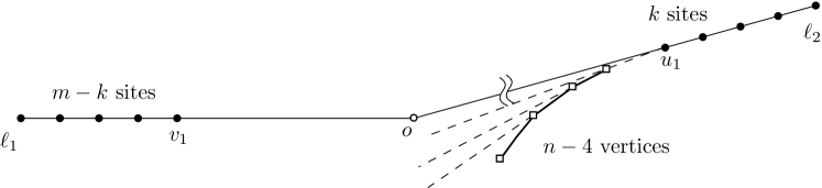
Figure 7: An example of which the order-$k$ Voronoi diagram has complexity of $\Omega(k(m-k)+\min\{nk,n(m-k)\})$.

Figure 7 shows an example of which the order-$k$ Voronoi diagram has complexity of $\Omega(k(m-k)+\min\{nk,n(m-k)\})$. Let $o$ be an arbitrary point in the plane. We construct a simple polygon $P$ and a set of sites with respect to the point $o$. Let $\ell_{1}$ be a sufficiently long horizontal line segment whose right endpoint is $o$ and $\ell_{2}$ be a sufficiently long line segment with a positive slope whose left endpoint is $o$. ($\ell_{1}$ and $\ell_{2}$ are not parts of the simple polygon, but they are auxiliary line segments to locate the points.) We put $m-k$ sites on $\ell_{1}$ such that the sites are sufficiently close to each other. Similarly, we put $k$ sites on $\ell_{2}$ such that sites are sufficiently close to each other and $\|v_{m-k}-o\|\ll\|u_{1}-o\|$, where $v_{i}$’s are sites on $\ell_{1}$ sorted along $\ell_{1}$ from $o$, $u_{j}$’s are sites on $\ell_{2}$ sorted along $\ell_{2}$ from $o$ for $i=1,\ldots,m-k$ and $j=1,\ldots,k$.

As a part of the boundary of $P$, we put a concave and $y$-monotone polygonal curve with $n-4$ vertices below $\ell_{2}$ such that the highest point of the curve is sufficiently close to $u_{1}$. Then we put another four vertices of $P$ sufficiently far from the sites such that $P$ contains all sites and there is no simple polygon containing more Voronoi vertices than $P$ contains.

Lemma 25.

For any $\kappa$ consecutive sites on $\ell_{1}$ with $1\leq\kappa\leq\min\{k,m-k\}$, there exist $k-\kappa$ sites on $\ell_{2}$ such that the $\kappa$ sites on $\ell_{1}$ and the $k-\kappa$ sites on $\ell_{2}$ define a non-empty Voronoi cell.

Proof.

Consider $\kappa$ consecutive sites $v_{i},\ldots,v_{i+\kappa-1}$ on $\ell_{1}$. We show that there is a point whose nearest $k$ sites are $v_{i},\ldots,v_{i+\kappa-1}$ and $u_{1},\ldots,u_{k-\kappa}$. To show this, consider the point $x$ equidistant from $v_{i},v_{i+\kappa-1}$ and $u_{k-\kappa}$. Since $\|v_{m-k}-o\|\ll\|u_{1}-o\|$, it holds that $\|x-u_{k-\kappa}\|\geq\|x-u_{j}\|$ for any index $j\leq k-\kappa$ and $\|x-u_{k-\kappa}\|\leq\|x-u_{j}\|$ for any index $j\geq k-\kappa$. This implies that the nearest $k$ sites from $x$ is $v_{i},\ldots,v_{i+\kappa-1}$ and $u_{1},\ldots,u_{k-\kappa}$. Therefore, the lemma holds. ∎

Lemma 26.

For every integer $\kappa$ with $1\leq\kappa\leq\min\{k,m-k\}$, there are $\Theta(n)$ Voronoi edges which come from the bisecting curve of $v_{\kappa}$ and $u_{k-\kappa}$.

Proof.

Consider the bisecting curve of $v_{\kappa}$ and $u_{k-\kappa}$. Due to the concave curve with $n-4$ vertices, the bisecting curve consists of $O(n)$ hyperbolic arcs and one line segment. We claim that each hyperbolic arc is a Voronoi edge of $k\textnormal{-}\textsf{VD}$. To see this, for any point $p$ in a hyperbolic arc of the bisecting curve, observe that $d(v_{\kappa},p)\leq d(v_{i},p)$ for any $i\geq\kappa$ and $d(u_{k-\kappa},p)\leq d(u_{j},p)$ for any $j\geq k-\kappa$. This is because $p$ lies below $\ell_{1}\cup\ell_{2}$. Therefore, there are $O(n)$ Voronoi edges from the bisecting curve of $v_{\kappa}$ and $u_{k-\kappa}$. ∎

Lemma 25 implies that $k\textnormal{-}\textsf{VD}$ contains $\Omega(k(m-k))$ cells, and Lemma 26 implies that $k\textnormal{-}\textsf{VD}$ contains $\Omega(\min\{nk,n(m-k)\})$ edges.

An upper bound.

As Liu and Lee [12] shows, each Voronoi vertex of $k\textnormal{-}\textsf{VD}$ has degree 2 or 3, except for the vertices lying on the boundary of $P$. In the following, we show that $k\textnormal{-}\textsf{VD}$ has $O(k(m-k)+\min\{nk,n(m-k)\})$ Voronoi edges, which implies that the complexity of $k\textnormal{-}\textsf{VD}$ is $O(k(m-k)+\min\{nk,n(m-k)\})$ by the Euler’s formula for planar graphs.

A Voronoi edge is a part of the bisecting curve of two sites. Consider Voronoi edges that come from the bisecting curve of two sites $s_{1}$ and $s_{2}$ in $S$. Such Voronoi edges form a curve that connects two degree-3 (or degree-1) vertices $v$ and $u$. Let $V(s_{1},s_{2})$ is the set of vertices of $P$ in $\pi(s_{1}^{\prime},v)\cup\pi(s_{1}^{\prime},u)\cup\pi(s_{2}^{\prime},v)\cup\pi(s_{2}^{\prime},u)$ excluding $s_{1}^{\prime}$ and $s_{2}^{\prime}$, where $s_{i}^{\prime}$ is the junction of $\pi(s_{i},u)$ and $\pi(s_{i},v)$ for $i=1,2$. Recall that the number of Voronoi edges on the common boundary of $V_{1}$ and $V_{2}$ is $O(1+|V(s_{1},s_{2})|)$. (Refer to Figure 5(b).)

For each vertex $w$ of $P$, we focus on the number of pairs $(s_{1},s_{2})$ of sites such that $w$ is contained in $V(s_{1},s_{2})$. Observe that either $s_{1}$ or $s_{2}$ (but not both) is one of the $k$ nearest sites from $w$. Without loss of generality, we assume that $s_{1}$ is one of the $k$ nearest sites from $w$. We claim that there is no site $s_{3}$ distinct from $s_{1}$ such that $w\in V(s_{2},s_{3})$. This is because $\pi(s_{2},x)$ intersects at most one Voronoi edge defined by $s_{2}$ and some other site for any point $x$ in $P$. We also claim that there is no site $s_{3}$ distinct from $s_{2}$ such that $w\in V(s_{1},s_{3})$. Assume to the contrary that there is such a site $s_{3}$. We observe that $s_{1}$ is one of the $k$ nearest sites of any point in the region $R$ bounded by $\pi(s_{1}^{\prime},v)\cup\pi(s_{1}^{\prime},u)$ and $b(s_{1},s_{2})$. A Voronoi edge defined by $s_{1}$ and $s_{3}$ does not intersect $R$. This means that $V(s_{1},s_{2})$ and $V(s_{1},s_{3})$ are interior disjoint. Thus $w$ is the junction of $\pi(s_{1},u^{\prime})$ and $\pi(s_{2},v^{\prime})$, where $u^{\prime}$ and $v^{\prime}$ are the endpoints of the Voronoi edge defined by $s_{1}$ and $s_{2}$. Thus it is not contained in $V(s_{1},s_{3})$, which is a contradiction. By the two claims, the number of pairs $(s,s^{\prime})$ with $w\in V(s,s^{\prime})$ is $\min\{k,m-k\}$ for each vertex $w$ of $P$.

Therefore, the number of Voronoi edges is $O(k(m-k)+\min\{nk,n(m-k)\})$, and the total complexity of $k\textnormal{-}\textsf{VD}$ is $O(k(m-k)+\min\{nk,n(m-k)\})$.

Combining the lower bound example, we have the following lemma.

Lemma 27.

The geodesic order-$k$ Voronoi diagram of $m$ points contained in a simple polygon with $n$ vertices has complexity of $\Theta(k(m-k)+\min\{nk,n(m-k)\})$.

6.2 Computing the Topological Structure of the Diagram

We use the notations defined in Section 5. For VD, we maintain the combinatorial structure of the beach line as $x$ moves along $\partial P$. For $k\textnormal{-}\textsf{VD}$, we maintain the combinatorial structures of $k$ curves each of which represents a level of the arrangement of some curves.

For a site $s\in P(x)$, recall that $R_{s}(x)=\{p\in P(x):d(p,s)\leq d(p,\pi(o,x))\}$ is connected. Moreover, the boundary of $R_{s}(x)$ consists of one polygonal chain of $\partial P$ and a simple curve with endpoints on $\partial P$. We call the simple curve the wave-curve for $s$. A wave-curve is weakly monotone with respect to $\pi(o,x)$ by Lemma 14.

We say that a point $p\in P(x)$ lies above a curve if $\pi(p,\pi(o,x))$ intersects the curve. We use $L_{i}(x)$ to denote the region of $P(x)$ consisting of all points lying above at least $i$ wave-curves for sites contained in $P(x)$. The $i$th-level of the arrangement of wave-curves of sites contained in $P(x)$ is defined to be the boundary of $L_{i}(x)$ excluding $\partial P$. The $i$th-level for each $i$ is weakly monotone with respect to $\pi(o,x)$ and consists of at most $m$ simple curves with endpoints lying on $\partial P$. Note that the beach line for VD coincides with the 1st-level of the arrangement of the wave-curves for all sites in $P(x)$ and $R(x)$ coincides with $L_{1}(x)$.

Lemma 28.

$k\textnormal{-}\textsf{VD}[S]$ restricted to $L_{k}(x)$ coincides with $k\textnormal{-}\textsf{VD}[S\cap P(x)]$ restricted to $L_{k}(x)$.

Proof.

Consider a Voronoi cell of $k\textnormal{-}\textsf{VD}[S]$ containing a point $p\in L_{k}(x)$. We show that this cell is associated with $k$ sites in $S\cap P(x)$. To see this, observe that $d(p,s)>d(p,\pi(o,x))$ for any site $s\notin P(x)$. By the definition of $L_{k}(x)$, there are $k$ sites in $P(x)$ whose geodesic distance from $p$ is at most $d(p,\pi(o,x))$. Thus the Voronoi cell of $k\textnormal{-}\textsf{VD}[S]$ containing $p$ is associated with $k$ sites in $S\cap P(x)$. Therefore, the lemma holds. ∎

Therefore, we can obtain the topological structure of $k\textnormal{-}\textsf{VD}[S]$ by maintaining the topological structure of the $k$th-level of the arrangement of wave-curves. In addition to this, we maintain the topological structures of the $i$th-level of the arrangement for all $i<k$ to detect the changes to the topological structure of the $k$th-level. A breakpoint of the $i$th-level is an intersection of two wave-curves for each $i=1,\ldots,k$, and an endpoint of the $i$th-level is an endpoint of a maximal connected curve in the $i$th-level. Let $B_{i}$ be the sequence of breakpoints and endpoints of the $i$th-level, which represents the combinatorial structure of the $i$th-level.

To avoid the case that $R(x)$ does not contain $P$ after the sweep, we consider a simple polygon $P^{\prime}$ obtained from $P$ by attaching a long and very thin triangle on $\partial P$ as we do in Section 5.

Events.

There are four types of events: site events, circle events, vanishing events and merging events. Every event corresponds to a key which is a point on $\partial P^{\prime}$. An event occurs when the sweep point $x$ passes through its corresponding key. The definitions of the event types are analogous to the ones in Section 5.

Each site $s$ in $S$ defines a site event. The key of the site event defined by $s$ is the point on $\partial P^{\prime}$ that comes first from $o$ in clockwise order along $\partial P^{\prime}$ among the points $x^{\prime}$ with $s\in\pi(o,x^{\prime})$. A pair $(\beta_{1},\beta_{2})$ of consecutive breakpoints in $B_{i}$ defines a circle event if there exists the point $c$ equidistant from three sites defining $\beta_{1}$ or $\beta_{2}$. The key of this circle event is the point on $\partial P^{\prime}$ that comes first from $o$ in clockwise order along $\partial P^{\prime}$ among the points $x^{\prime}$ with $d(c,\pi(o,x^{\prime}))=d(c,p)$, where $p$ is one of the sites defining $\beta_{1}$ or $\beta_{2}$. Each breakpoint $\beta$ in $B_{i}$ defines a vanishing event. Let $(s_{1},s_{2})$ be the pair defining $\beta$. Let $p$ be the point on $\partial P^{\prime}$ equidistant from $s_{1}$ and $s_{2}$ that lies outside of $L_{i}(x)$. The key $k$ of the vanishing event is the point on $\partial P^{\prime}$ that comes first from $o$ in clockwise order along $\partial P^{\prime}$ among the points $x^{\prime}$ with $d(p,\pi(o,x^{\prime}))=d(p,s_{1})$. A pair $(\beta_{1},\beta_{2})$ of consecutive endpoints in $B_{i}$ defines a merging event if $\beta_{1}$ and $\beta_{2}$ are endpoints of different connected curves of the $i$th-level. Let $s_{1}$ and $s_{2}$ be the sites defining $\beta_{1}$ and $\beta_{2}$, respectively. Let $p$ be the (unique) point on $\partial P^{\prime}$ equidistant from $s_{1},s_{2}$ that comes after $\beta_{1}$ and before $\beta_{2}$ from $o$ along $\partial P$ in clockwise order. The key $k$ of the merging event defined by $(\beta_{1},\beta_{2})$ is the point on $\partial P^{\prime}$ that comes first from $o$ in clockwise order along $\partial P^{\prime}$ among the points $x^{\prime}$ with $d(p,\pi(o,x^{\prime}))=d(p,s_{1})$.

The changes of $B_{i}$ due to events are analogous to the ones in Section 5, except for the circle events. The sequence $B_{i}$ may change when the sweep point passes through the key of some circle event defined by a pair of consecutive breakpoints in $B_{i-1}$ or $B_{i-2}$ as illustrated in Figure 8.

An algorithm.

Initially, $B_{i}$ is empty for all $i=1,\ldots,k$, so there is no event. We compute all site events in advance. For each site, we can compute its key in $O(\log n)$ time [8]. As we handle events, the sequence $B_{i}$ changes accordingly and we reflect these changes to $B_{i}$. At the same time, we compute the topological structure of $k\textnormal{-}\textsf{VD}$ using $B_{k}$.

To handle a site event defined by a site $s$, we find the position for $s$ in $B_{i}$ and add $s$ to $B_{i}$ for each $i\leq k$. This takes $O(\log^{2}n\log|B_{i}|)$ time for each $i$ by Lemma 19. Adding $s$ to $B_{i}$ makes new pairs of consecutive breakpoints or endpoints in $B_{i}$, or new breakpoints, which define some events. We compute the key for each event in $O(\log^{2}n)$ time using Lemma 17.

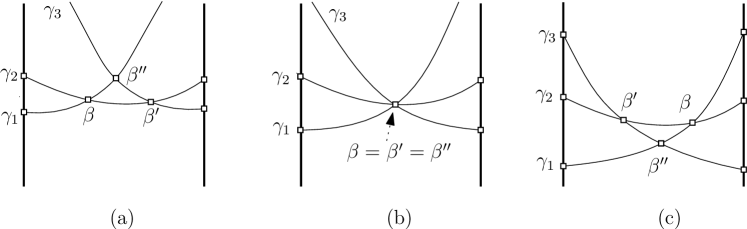
Figure 8: The curves $\gamma_{1}$, $\gamma_{2}$, and $\gamma_{3}$ are wave-curves of $s_{1},s_{2}$, and $s_{3}$, respectively. The points $\beta,\beta^{\prime}$, and $\beta^{\prime\prime}$ are breakpoints defined by $(s_{1},s_{2}),(s_{2},s_{3})$, and $(s_{3},s_{1})$, respectively.

To handle a circle event defined by a pair $(\beta,\beta^{\prime})$ of consecutive breakpoints in $B_{i}$, we consider the following observations, which are analogous to the ones for Euclidean order-$k$ Voronoi diagram given by Zavershynskyi and Papadopoulou [18]. Let $(s_{1},s_{2})$ and $(s_{2},s_{3})$ be the pairs of sites defining $\beta$ and $\beta^{\prime}$, respectively. Let $c$ be the point equidistant from $s_{1},s_{2}$ and $s_{3}$, and $k$ be the key of the event. When the sweep point $x$ passes through $k$, two breakpoints merge into a breakpoint defined by $(s_{1},s_{3})$ in $B_{i}$. For illustration, see Figure 8.

Additionally, $B_{i+1}$ and $B_{i+2}$ change. The breakpoints $\beta$ and $\beta^{\prime}$ are also in $B_{i+1}$ before $x$ reaches $k$. Moreover, a breakpoint $\beta^{\prime\prime}$ defined by $(s_{1},s_{2})$ lies between $\beta$ and $\beta^{\prime}$ in $B_{i+1}$. When $x$ reaches $k$, the three breakpoints merge into one (degenerate) breakpoint equidistant from $s_{1},s_{2}$ and $s_{3}$. After $x$ passes through $k$, the order of the breakpoints changes: $\beta^{\prime},\beta^{\prime\prime}$ and $\beta$. For $B_{i+2}$, there is $\beta^{\prime\prime}$ before $x$ reaches $k$. After $x$ passes through $k$, $\beta^{\prime\prime}$ is replaced with $\beta^{\prime}$ and $\beta$. The remaining levels do not change as $x$ passes through $x^{\prime}$. We update $B_{i}$, $B_{i+1}$ and $B_{i+2}$ accordingly in $O(\log|B_{i}|+\log|B_{i+1}|+\log|B_{i+2}|)$ time.

After updating $B_{i}$, $B_{i+1}$ and $B_{i+2}$, we have new pairs of consecutive breakpoints or endpoints, or new breakpoints. We compute the events defined by them and add the events to the event queue in $O(\log^{2}n+\log|B_{i}|+\log|B_{i+1}|+\log|B_{i+2}|)$ time. The other events can be handled in a way similar to the one in Section 5 in $O(\log^{2}n+\log|B_{i}|)$ time.

An analysis.

We have $m$ site events and spend $O(\sum_{1\leq i\leq k}\log^{2}n\log|B_{i}|)$ time to handle each site event, where $|B_{i}|$ is the maximum length of $B_{i}$ during the sweep. We can handle all site events in $O(km\log^{2}n\log m)$ time in total by the following lemma.

Lemma 29.

The length of $B_{i}$ is $O(im)$ at any time.

Proof.

For $i=1$, the lemma holds by Lemma 21. Consider $i\geq 2$. Initially, $B_{i}$ is empty. When the sweep point passes through the key of a site event, the length of $B_{i}$ increases by at most two. When the sweep point passes through the key of a circle, vanishing, or merging event caused by $B_{i}$, the length of $B_{i}$ decreases. In contrast to the nearest-point Voronoi diagram, there is one more case that the length of $B_{i}$ increases in the higher-order Voronoi diagram. A circle event due to $B_{i-1}$ or $B_{i-2}$ (or, $B_{i-1}$ for $i=2$) increases the length of $B_{i}$ by at most one. Note that a circle event due to $B_{j}$ that is valid when the sweep point passes through its key corresponds to a degree-3 Voronoi vertex of $j$-VD. Thus there are $O(im)$ circle events due to $B_{i-1}$ or $B_{i}$ that are valid when the sweep point passes through their keys. Therefore, the length of $B_{i}$ is $O(im)$, and the lemma holds. ∎

There are $O(k^{2}m)$ circle events in total that are valid when the sweep point passes through their keys. This is because each such circle event corresponds to a degree-3 Voronoi vertex of $i$-VD for some $i$. There are $O(k^{2}m)$ vanishing or merging events in total that are valid when the sweep point passes through their keys. This is because each such event corresponds to a degree-1 Voronoi vertex. Recall that $i$-VD has $O(i(n-i))$ degree-1 or degree-3 vertices. Since we can handle each event in $O(\log m\log^{2}n)$ time, the running time for this algorithm is $O(k^{2}m\log m\log^{2}n)$ time.

Therefore, we have the following lemma and theorem.

Lemma 30.

After constructing the shortest path data structure for $P^{\prime}$ and the shortest path map for $P^{\prime}$ from any fixed point, we can compute $k\textnormal{-}\textsf{VD}$ in $O(k^{2}m\log m\log^{2}n)$ time using $O(km)$ space (excluding the two data structures).

Theorem 31.

Given a set of $m$ points contained in a simple polygon with $n$ vertices, we can compute the geodesic order-$k$ Voronoi of the points in $O(k^{2}m\log m\log^{2}n+\min\{nk,n(m-k)\})$ time using $O(n+km)$ space.

7 The Geodesic Farthest-Point Voronoi Diagram

In this section, we present two algorithms for computing the topological structure of FVD: an $O(n+m\log m+m\log^{2}n)$-time algorithm and an $O(m\log m\log^{2}n)$-time algorithm. The latter algorithm assumes that we have the shortest path data structure for $P$. The former algorithm is faster than the latter because computing the shortest path data structure for $P$ takes $O(n)$ time. However, the latter algorithm has an advantage if we compute FVD several times with different point sets. For an application, see Section 37.

The algorithm given by Aronov et al.

Aronov et al. [3] showed that FVD forms a tree whose root is the geodesic center $c$ of the sites. They first compute $c$ and the geodesic convex hull of the sites. Then they compute FVD restricted to the boundary of the polygon in $O((n+m)\log(n+m))$ time. That is, they compute all degree-1 vertices of FVD.

Then they compute the edges of FVD towards the geodesic center by a reverse geodesic sweep method. They showed that $d(u,c)\leq d(v,c)$ for any ancestor $u$ of a Voronoi vertex $v$ in FVD (a tree). Thus they compute the Voronoi edges of FVD from the boundary of $P$ toward $c$ one by one. This takes $O((n+m)\log(n+m))$ time.

Computing the geodesic center of the sites and the geodesic convex hull of the sites.

We follow the framework of the algorithm by Aronov et al. [3], but we can achieve a faster algorithm for $m\leq n/\log^{2}n$ by applying their approach to compute the topological structure of FVD. We first compute the geodesic center of the sites in $S$. This takes $O(n+m\log m)$ time [1, 9], or $O(m\log m\log^{2}n)$ time with the shortest path data structure for $P$ by Theorem 9. The geodesic convex hull of the sites can be computed in $O(n+m\log m)$ time [9].

Computing the diagram restricted to the boundary of the polygon

We can compute FVD restricted to the boundary of $P$ in $O(n+m)$ time using the algorithm by Oh et al. [15] once we have the sequence of the sites along the boundary of the geodesic convex hull. The algorithm uses the property that the order of the sites along the boundary of the geodesic convex hull of them is the same as the order for their Voronoi cells along the boundary of the polygon, which is shown by Aronov et al [3]. They consider the sites on the boundary of the geodesic convex hull one by one and compute the FVD restricted to the boundary of $P$ along the boundary. Combining their approach with Lemma 18, we can compute FVD restricted to the boundary of $P$ in $O(m\log^{2}n)$ time.

Extending the diagram inside the polygon

We apply the reverse geodesic sweep from the boundary of $P$ towards the center $c$ of the sites. In this problem, a sweep line is a simple curve consisting of points equidistant from $c$. Let $B$ be the (circular) sequence of the sites that have their Voronoi cells on the sweep line in clockwise order. As an exception, in the initial state, we set $B$ to be the sequence of the sites whose Voronoi cells appear on $\partial P$.

No site, vanishing, or merging event occurs during the sweep because FVD forms a tree. So we handle the circle event only. Every triple of consecutive sites in $B$ defines a circle event. The key defined by a triple of sites is $d(c,c^{\prime})$ for the point $c^{\prime}$ equidistant from the three sites. Thus, we can compute the key of each triple of consecutive sites in $B$ in $O(\log^{2}n)$ time.

The analysis is similar to the one in Section 5. There are $O(m)$ events in total, and each event can be handled in $O(\log m+\log^{2}n)$ time. Thus extending the diagram inside the polygon takes $O(m\log m+m\log^{2}n)$ time.

Lemma 32.

We can compute the topological structure of FVD in $O(m\log m\log^{2}n)$ or $O(n+m\log m+m\log^{2}n)$ time once the shortest path data structure for $P$ is constructed.

Theorem 33.

Given a set of $m$ point sites contained in a simple polygon with $n$ vertices, we can compute the geodesic farthest-point Voronoi diagram of the points in $O(n+m\log m+m\log^{2}n)$ time using $O(n+m)$ space.

8 Dynamic Data Structures for Nearest or Farthest Point Queries

We showed that the topological structure of a Voronoi diagram can be computed without considering the whole polygon once we have the shortest path data structure for $P$. The topological structure can also be used for data structures for answering nearest or farthest point queries for a dynamic point set.

We apply the framework given by Bentley and Saxe [4]. At all times, we maintain $O(\sqrt{m})$ disjoint sets each of which consists of $O(\sqrt{m})$ points. For each set, we compute the topological structure of the nearest-point (or the farthest-point) Voronoi diagram of the points in the set. This takes $O(\sqrt{m}\log m\log^{2}n)$ time. For a nearest (or a farthest) point query, we simply find the Voronoi cell containing the query point for each of $O(\sqrt{m})$ Voronoi diagrams. Then we have $O(\sqrt{m})$ candidates for the nearest (or the farthest) point from the query point. We find the nearest (or the farthest) point from the query point directly among them.

While processing updates, we maintain the invariant that every set, except only one, contains at most $2\sqrt{m}$ and at least $\sqrt{m}/2$ points at any time, where $m$ is the number of the points in the moment. For the insertion of a point $p$, we choose the set of smallest size. If the set contains more than $2\sqrt{m}$ points, we split it into two equal sized sets, add $p$ to one of them, and reconstruct the Voronoi diagram for each set. Otherwise, we add $p$ to the set of smallest size and reconstruct the Voronoi diagram for this set. The invariant holds for any case. For the deletion of a point $p$, we find the set containing $p$ and remove $p$ from the set. If there are two sets containing less than $\sqrt{m}/2$ points, we merge them into one and reconstruct the Voronoi diagram for the set. The invariant still holds. By the invariant, we have $O(\sqrt{m})$ sets at any time. For each update, we reconstruct the Voronoi diagrams of at most two sets containing at most $2\sqrt{m}$ points. Thus the update time is $O(\sqrt{m}\log m\log^{2}m)$.

To answer a query, we find the Voronoi cell containing the query point using the topological structure of a Voronoi diagram. To do this, when computing the adjacency graph, we also construct a data structure that supports a point location query as follows.

Point location.

The key idea is to approximate the Voronoi diagram into a polygonal subdivision using its adjacency graph and the exact positions of degree-1 and degree-3 vertices. Consider an edge of the adjacency graph corresponding to two adjacent Voronoi cells $V_{1}$ and $V_{2}$. We say that a polygonal curve approximates the common boundary of $V_{1}$ and $V_{2}$ if it connects the two endpoints of the common boundary, consists of at most three line segments, and is contained in the closure of $V_{1}\cup V_{2}$.

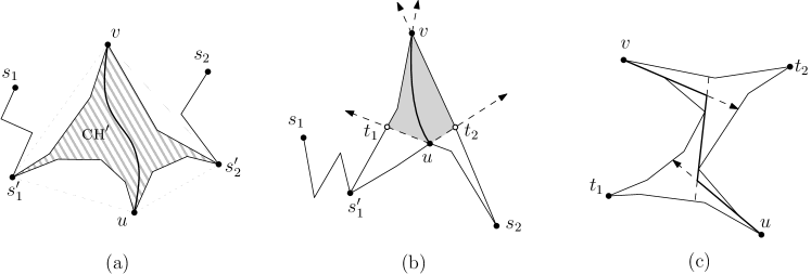
Figure 9: (a) The common boundary of the Voronoi cells with sites $s_{1}$ and $s_{2}$ is contained in the convex hull $\textsc{ch}^{\prime}$ (dashed region) of $s_{1}^{\prime},s_{2}^{\prime},u$ and $v$. (b) For the farthest-point Voronoi diagram, we extend four edges to find a region that is contained in the closure of $V_{1}\cup V_{2}$ and is bounded by four concave curves. (c) Given a region bounded by four concave curves, we can find a polygonal curve approximating the common boundary.

Lemma 34.

We can compute a polygonal curve approximating the common boundary of two adjacent Voronoi cells in $O(\log n)$ time.

Proof.

Let $u$ and $v$ be the endpoints of the common boundary of two adjacent Voronoi cells $V_{1}$ and $V_{2}$. Let $s_{i}$ be the site associated with $V_{i}$ and $s_{i}^{\prime}$ be the junction of $\pi(s_{i},u)$ and $\pi(s_{i},v)$ for $i=1,2$. The junction of $\pi(u,s_{1})$ and $\pi(u,s_{2})$ is $u$ itself, and the junction of $\pi(v,s_{1})$ and $\pi(v,s_{2})$ is $v$ itself under the general position condition. See figure 9(a) and (b). Therefore, the geodesic convex hull, denoted by $\textsc{ch}^{\prime}$, of $s_{1}^{\prime},s_{2}^{\prime},u$ and $v$ consists of at most four maximal concave curves.

Using this fact, we first find two points $t_{1},t_{2}$ such that the geodesic convex hull ch of $t_{1},t_{2},u,v$ is contained in the closure of $V_{1}\cup V_{2}$ and the boundary of ch consists of at most four maximal concave polygonal curves. Then we compute a polygonal curve approximating the common boundary in ch.

We first show how to find such points $t_{1}$ and $t_{2}$. Consider the case that $V_{1}$ and $V_{2}$ are two adjacent Voronoi cells in the nearest-point Voronoi diagram. Observe that $\pi(s_{i}^{\prime},u)\cup\pi(s_{i}^{\prime},v)\subseteq V_{i}$ for $i=1,2$. Thus, $\textsc{ch}^{\prime}$ is contained in the closure of $V_{1}\cup V_{2}$. Since the boundary of $\textsc{ch}^{\prime}$ consists of at most four concave polygonal curves, $\pi(s_{i}^{\prime},u),\pi(s_{i}^{\prime},v)$ for $i=1,2$, the two points $s_{1}^{\prime}$ and $s_{2}^{\prime}$ satisfy the condition for $t_{1}$ and $t_{2}$, respectively.

For the case that $V_{1}$ and $V_{2}$ are two adjacent Voronoi cells in the farthest-point Voronoi diagram, consider two line segments contained in $P$ with endpoint $u$ such that each of them is collinear to the edge of $\pi(s_{i},u)$ incident to $u$ for $i=1,2$. Similarly, we consider two line segments contained in $P$ with endpoint $v$ such that each of them is collinear to the edge of $\pi(s_{i},v)$ incident to $v$ for $i=1,2$. If $u$ or $v$ is on $\partial P$, the line segments are $u$ or $v$ itself. It is known that the line segments incident to $u$ are contained in $V_{1}$ and the other two line segments are contained in $V_{2}$ [3]. The four line segments subdivide $P$ into subpolygons. Let $Q$ denote the subpolygon that contains the common boundary of $V_{1}$ and $V_{2}$. If $u$ and $v$ are on $\partial P$, the subpolygon $Q$ is the whole polygon $P$. Then $Q$ is contained in the closure of $V_{1}\cup V_{2}$. See Figure 9(b).

Consider the intersection $Q\cap\textsc{ch}^{\prime}$. For $i=1,2$, if $s_{i}^{\prime}$ is contained in $Q$, both $\pi(s_{i}^{\prime},u)$ and $\pi(s_{i}^{\prime},v)$ appear on the boundary of $Q\cap\textsc{ch}^{\prime}$, and we set $t_{i}=s_{i}^{\prime}$. Otherwise, only one of them, say $\pi(s_{i}^{\prime},v)$, crosses one of the line segment appearing on the boundary of $Q$. We set the cross point to $t_{i}$. See Figure 9(b). Therefore, $Q\cap\textsc{ch}^{\prime}$ is the geodesic convex hull of $t_{1},t_{2},u$ and $v$ whose boundary consists of at most four maximal concave polygonal curves, $\pi(t_{i},u)$ and $\pi(t_{i},v)$ for $i=1,2$. Moreover, we can compute $t_{i}$ in $O(\log n)$ time using Lemma 2.

Now, we have two points $t_{1},t_{2}$ such that the geodesic convex hull ch of $t_{1},t_{2},u,v$ is contained in the closure of $V_{1}\cup V_{2}$ and consists of at most four maximal concave polygonal curves. Since $\pi(u,v)\subset\textsc{ch}$, we approximate $\pi(u,v)$ by a polygonal curve consisting of at most three segments contained in ch as follows. If $\pi(u,v)$ is a line segment, it is the polygonal curve. Otherwise, we can compute a polygonal curve consisting of at most three line segments from the extensions of the two edges of $\pi(u,v)$, one incident to $u$ and one incident to $v$, towards the other endpoints of $\pi(u,v)$, and one line segment tangent to $\pi(t_{1},v)$ and $\pi(t_{2},u)$. See Figure 9(c). This can be done in $O(\log n)$ time using the shortest path data structure for $P$. This proves the lemma for both the nearest-point and farthest-point Voronoi diagrams. ∎

Since each polygonal curve approximating the common boundary of two adjacent Voronoi cells described in Lemma 34 is contained in the closure of the union of the Voronoi cells, the following property is satisfied.

Corollary 35.

No two polygonal curves constructed by Lemma 34 cross each other.

The following lemma allows us to construct a data structure on a adjacency graph that supports a point location query efficiently. In the lemma, we assume that we have a ray-shooting data structure for $P$.

Lemma 36.

We can construct a data structure for the topological structure of the nearest-point (or the farthest-point) Voronoi diagram of $O(\sqrt{m})$ points in $O(\sqrt{m}\log(n+m))$ time that supports a point location query for the Voronoi diagram in $O(\log(n+m))$ time.

Proof.

We first approximate every common boundary of two adjacent Voronoi cells by a polygonal curve, which takes $O(\sqrt{m}\log n)$ time in total. Then we have $O(\sqrt{m})$ polygonal curves each of which consists of at most three line segments. Let $A$ be the set of all line segments of the curves. As a preprocessing, we construct a ray-shooting data structure for $A$ in $O(\sqrt{m}\log m)$ time using $O(\sqrt{m})$ space.

We show how to find the Voronoi cell containing a query point $q$. Consider the subdivision $\mathcal{P}_{A}$ of $P$ with respect to $A$. Note that the complexity of $\mathcal{P}_{A}$ is $O(\sqrt{m}+n)$. We first find the region in $\mathcal{P}_{A}$ containing $q$ as follows without constructing $\mathcal{P}_{A}$ explicitly. Let $r$ be the ray from $q$ going upwards. We find the line segment in $A$ that $r$ hits first using the ray-shooting data structure constructed on $A$ in $O(\log m)$ time. Then we find the edge of $P$ that $r$ hits first in $O(\log n)$ time. By comparing the vertical distances from $q$ to the edge of $P$ and the line segment in $A$, we can determine the edge of $\mathcal{P}_{A}$ that $r$ hits first. Thus we can find the region in $\mathcal{P}_{A}$ containing $q$ in $O(\log(n+m))$ time. (If $r$ hits an edge of $P$ before hitting any approximate polygonal curve, we determine which region in $\mathcal{P}_{A}$ contains $q$ in $O(\log(n+m))$ time by sorting the degree-1 vertices along $\partial P$ in advance.)

Let $s$ be the site associated with the region we just found. Since we consider only the subdivision $\mathcal{P}_{A}$, $s$ might not be the nearest-point (or the farthest-point) from $q$. In this case, $s$ is contained in a region bounded by a chain $\gamma$ of Voronoi edges defined by $s$ and $s^{\prime}$, and a chain $\tilde{\gamma}$ approximating $\gamma$. Note that $s^{\prime}$ is the nearest-point (or the farthest-point) of $q$. This is because a polygonal curve approximating the common boundary of two Voronoi cells is contained in the union of them, and no two curves constructed from Lemma 34 cross each other.

We show how to find $s^{\prime}$. For a nearest-point query, the ray from $q$ in direction opposite to the edge of $\pi(s,q)$ incident to $q$ does not intersect $\gamma$. Since $q$ is contained in the region bounded by $\gamma$ and $\tilde{\gamma}$, but the ray does not intersect $\gamma$, the ray intersects $\tilde{\gamma}$. We compute $\tilde{\gamma}$ by finding the point where the ray hits first in $\mathcal{P}_{A}$ as we did before, and find the site $s^{\prime}$ defining $\tilde{\gamma}$ other than $s$. By comparing $d(s,q)$ and $d(s^{\prime},q)$, we get the answer in $O(\log(n+m))$ time.

For a farthest-point query, we do in a similar way. In this case, the extension of the edge of $\pi(s,q)$ incident to $q$ in direction opposite to $q$ does not intersect $\gamma$, and thus it intersects $\tilde{\gamma}$. We find the edge of $\mathcal{P}_{A}$ that intersects the extension in $O(\log(n+m))$ time, and compute $s^{\prime}$ in a way similar to the one for a nearest-point query. Then by comparing $d(s,q)$ and $d(s^{\prime},q)$, we get the answer in $O(\log(n+m))$ time. ∎

We perform the point location query on each of the $O(\sqrt{m})$ Voronoi diagrams as described in Lemma 36 and find the nearest (or the farthest) point from the query point among the $O(\sqrt{m})$ solutions, which takes $O(\sqrt{m}\log(n+m))$ time. For the update, we need to compute the topological structure of the Voronoi diagram for the updated set, which takes $O(\sqrt{m}\log m\log^{2}n)$ time. Then we reconstruct the data structure for point location on the topological structure.

Theorem 37.

We can construct a data structure of size $O(n+m)$ that supports a nearest-point (or a farthest-point) query under point insertions and deletions. Each query takes $O(\sqrt{m}\log(n+m))$ time and each update takes $O(\sqrt{m}\log m\log^{2}n)$ time.

References

- [1] Hee-Kap Ahn, Luis Barba, Prosenjit Bose, Jean-Lou De Carufel, Matias Korman, and Eunjin Oh. A linear-time algorithm for the geodesic center of a simple polygon. Discrete & Computational Geometry, 56(4):836–859, 2016.
- [2] Boris Aronov. On the geodesic Voronoi diagram of point sites in a simple polygon. Algorithmica, 4(1):109–140, 1989.
- [3] Boris Aronov, Steven Fortune, and Gordon Wilfong. The furthest-site geodesic Voronoi diagram. Discrete & Computational Geometry, 9(1):217–255, 1993.
- [4] Jon Louis Bentley and James B. Saxe. Decomposable searching problems 1: Static-to-dynamic transformations. Journal of Algorithms, 1(4):297–396, 1980.
- [5] Bernard Chazelle. The Discrepancy Method. Cambridge University Press, 2000.
- [6] Bernard Chazelle, Herbert Edelsbrunner, Michelangelo Grigni, Leonidas Guibas, John Hershberger, Micha Sharir, and Jack Snoeyink. Ray shooting in polygons using geodesic triangulations. Algorithmica, 12(1):54–68, 1994.
- [7] Steven Fortune. A sweepline algorithm for Voronoi diagrams. Algorithmica, 2(1):153–174, 1987.
- [8] Leonidas Guibas, John Hershberger, Daniel Leven, Micha Sharir, and Robert E. Tarjan. Linear-time algorithms for visibility and shortest path problems inside triangulated simple polygons. Algorithmica, 2(1):209–233, 1987.
- [9] Leonidas J. Guibas and John Hershberger. Optimal shortest path queries in a simple polygon. Journal of Computer and System Sciences, 39(2):126–152, 1989.
- [10] John Hershberger. A new data structure for shortest path queries in a simple polygon. Information Processing Letters, 38(5):231–235, 1991.
- [11] David Kirkpatrick and Jack Snoeyink. Tentative prune-and-search for computing voronoi vertices. In Proceedings of the 9th Annual Symposium on Computational Geometry (SoCG 1993), pages 133–142, 1993.
- [12] Chih-Hung Liu and D.T.Lee. Higher-order geodesic Voronoi diagrams in a polygonal domain with holes. In Proceedings of the 24th Annual ACM-SIAM Symposium on Discrete Algorithms (SODA 2013), pages 1633–1645, 2013.
- [13] Nimrod Megiddo. Linear-time algorithms for linear programming in and related problems. SIAM Journal on Computing, 12(4):759–776, 1983.
- [14] Joseph S. B. Mitchell. Geometric shortest paths and network optimization. In Handbook of Computational Geometry, pages 633–701. Elsevier, 2000.
- [15] Eunjin Oh, Luis Barba, and Hee-Kap Ahn. The farthest-point geodesic voronoi diagram of points on the boundary of a simple polygon. In Proceedings of the 32nd International Symposium on Computational Geometry (SoCG 2016), pages 56:1–56:15, 2016.
- [16] Evanthia Papadopoulou and D.T.Lee. A new approach for the geodesic Voronoi diagram of points in a simple polygon and other restricted polygonal domains. Algorithmica, 1998(4):319–352, 1998.
- [17] Richard Pollack, Micha Sharir, and Günter Rote. Computing the geodesic center of a simple polygon. Discrete & Computational Geometry, 4(6):611–626, 1989.
- [18] Maksym Zavershynskyi and Evanthia Papadopoulou. A sweepline algorithm for higher order voronoi diagrams. In Proceedings of the 10th International Symposium on Voronoi Diagrams in Science and Engineering (ISVD 2013), pages 16–22, 2013.