Accuracy of noisy Spike-Train Reconstruction: a Singularity Theory point of view

Abstract

This is a survey paper discussing one specific (and classical) system of algebraic equations - the so called “Prony system”. We provide a short overview of its unusually wide connections with many different fields of Mathematics, stressing the role of Singularity Theory. We reformulate Prony System as the problem of reconstruction of “Spike-train” signals of the form $F(x)=\sum_{j=1}^{d}a_{j}\delta(x-x_{j})$ from the noisy moment measurements. We provide an overview of some recent results of [2, 3, 1, 29, 8, 7, 10, 11, 53] on the “geometry of the error amplification” in the reconstruction process, in situations where the nodes $x_{j}$ near-collide. Some algebraic-geometric structures, underlying the error amplification, are described (Prony, Vieta, and Hankel mappings, Prony varieties), as well as their connection with Vandermonde mappings and varieties. Our main goal is to present some promising fields of possible applications of Singulary Theory.

To the Memory of Egbert Brieskorn. Among the most important events which inspired scientific interests of the third author was (in late 1960s) Brieskorn’s discovery that 28 Milnor’s exotic spheres can be described by simple algebraic equations, and (in early 1980s) participation in Brieskorn Singularities seminar in Bonn.

1 Introduction

In this paper we consider the classical Prony system of algebraic equations, with the real unknowns $a_{j},x_{j},\ j=1,\ldots,d,$ and with the right hand side formed by the known real “measurements” $m_{0},\ldots,m_{2d-1}$. This system has a form

$$\sum_{j=1}^{d}a_{j}x_{j}^{k}=m_{k},\ k=0,1,\ldots,2d-1.$$ (1.1)

We denote by $A=(a_{1},\ldots,a_{d})\in{\mathbb{R}}^{d}$ and $X=(x_{1},\ldots,x_{d})\in{\mathbb{R}}^{d},\ x_{1}\leq x_{2}\leq\ldots\leq x_{d},$ the unknowns in system (1.1), and denote by ${\cal P}^{A}_{d}$ (resp. ${\cal P}^{X}_{d}$) the “parameter spaces” of the unknowns $A$ and $X,$ respectively. ${\cal P}_{d}={\cal P}^{A}_{d}\times{\cal P}^{X}_{d}$ denotes the total parameter space of $(A,X)$. The space (isomorphic to ${\mathbb{R}}^{2d}$) of the right-hand sides $\mu=(m_{0},m_{1},\ldots,m_{2d-1})$ of (1.1) is denoted by ${\cal M}_{d}$.

In what follows we will usually identify $(A,X)$ with a “spike-train signal”

$$F(x)=\sum_{j=1}^{d}a_{j}\delta(x-x_{j}).$$ (1.2)

Clearly, the moments $m_{k}(F)=\int x^{k}F(x)dx,\ k=0,1,\ldots,$ are given by $m_{k}(F)=\sum_{j=1}^{d}a_{j}x_{j}^{k}$, so reconstructing $F$ from its $2d-1$ initial moments is equivalent to solving (1.1), with $m_{k}=m_{k}(F)$.

Prony system appears in many classical theoretical and applied mathematical problems. In Section 2 we discuss some of these appearances. Explicit solution of (1.1) was given already in [48] (see Section 3 below).

There exists a vast literature on Prony and similar systems. In particular, the bibliography in [5] (1981) contains more than 50 pages. Most of recent applications are in Signal Processing. As a very partial sample we mention that in [14] and in many other publications a method, essentially equivalent to solving Prony system, was used in reconstructing signals with a “finite rate of innovation”. In [45, 46] the applicability of Prony-type systems was extended to some new wide and important classes of signals. In [12, 21] multidimensional Prony systems were investigated via symmetric tensors, in particular, connecting them to the polynomial Waring problem. In [25] Prony system appears in a general context of Compressed Sensing. In [9, 6] Prony-like systems were used in reconstructing piecewise-smooth functions from their Fourier data. Finally, in [6] the same reconstruction accuracy as for smooth functions was demonstrated (thus confirming the Eckhoff conjecture).

Some applications of Prony system are of major practical importance, and various algorithms and numerical methods have been developed for its solution (see [47] and references therein). However, in a (very important) case when some of the nodes $x_{j}$ nearly collide, while the measurements are noisy, these collision singularities lead to major mathematical and numerical difficulties. In particular, this happens in the context of the “super-resolution problem”, which was investigated in many recent publications. See [2, 3, 1, 8, 7, 10, 11, 17, 18, 22, 24, 26, 41] as a small sample.

Notice that the Prony system (1.1) is linear (with the Vandermonde matrix on the “nodes” $X$) with respect to the “amplitudes” $A$, while it is highly nonlinear with respect to $X$. As the nodes collide (or near-collide), the Vandermonde determinant vanishes. Even knowing the position of the nodes, the reconstruction of the amplitudes is still ill-posed.

Thus singularities enter the solution process of the Prony system because of its geometric nature, no matter what solution method do we use. We believe that using the tools of Singularity Theory in this problem is well justified. In [53, 11] we study the algebraic nature of nodes collision. In particular, we include into consideration the “confluent Prony systems”, corresponding to signals with multiple nodes, and with the derivatives of the $\delta$-function. We also introduce and study in [11] the “bases of finite differences” in the signal space ${\cal P}_{d}$, which behave coherently as the nodes collide.

In the present paper we give, following [2, 3, 1, 29, 8, 7, 10, 11, 53], a somewhat different point of view on the problem, stressing the role of Singularity Theory in understanding of Prony systems with noisy right-hand side. Below we discuss the following main topics:

1. In case of near-colliding nodes the initial measurements errors may be strongly amplified in the solution, making it unfeasible. However, the possible error-affected solutions are not distributed uniformly, but rather tightly concentrated along certain algebraic sets, known a priori (“Prony varieties” - see Sections 7 and 5 below).

Prony varieties are generalizations (via “making free” the amplitudes $A$) of the Vandermonde mappings and varieties, introduced and studied in Singularity Theory in [4, 32] and other publications (see Section 4).

2. A related notion is that of “Prony scenarios” (Section 8), which predict the error behavior along the Prony curves. An important part here is the description of the combinatorics of real zeroes in polynomial pencils, actively studied in Singularity Theory - see [15, 33, 34, 35].

3. In the presence of the measurement noise, statistical estimations of feasible solutions can be used. These methods are considered in the literature as superior in accuracy, but their practical implementation is difficult, because of complicated nonlinear minimization problems involved. We expect that the tools developed in Singularity Theory for the study of “maxima of smooth functions”, “cut-loci”, and similar objects, can be useful here (Section 6.1).

4. In the case of the real nodes $X$ (mainly presented in this paper) hyperbolic polynomials become a central topic in all the problems above. Hyperbolic polynomials and related objects are actively studied in Singularity Theory (see [4, 15, 23, 32, 33, 34, 35] as a partial sample), and we expect some of the available results to be directly applicable to Prony systems.

Among other common topics with Singularity Theory we shortly discuss below rank stratification of the space of Hankel-type matrices, solving parametric linear systems, polynomial Waring problem, and finite differences. We hope that the connections presented will proof useful in both domains.

2 Some appearances of the Prony system

We outline here some prominent classical appearances of the Prony system.

2.1 Exponential Interpolation

This was the problem studied by Prony himself in [48]. We consider an interpolation problem for a given function $f(x)$ at the $2d$ consequent integer points $0,1,\ldots,2d-1$, with the interpolant being the sum of the exponents

$$\sum_{j=1}^{d}a_{j}e^{\zeta_{j}x}.$$

We can choose freely $2d$ parameters $a_{j},\zeta_{j}$, in order to fit the values $y_{k}=f(k),\ k=0,\ldots,2d-1.$ Substituting $x=k$, and denoting $e^{\zeta_{j}}$ by $x_{j}$ we get the Prony system of equations

$$\sum_{j=1}^{d}a_{j}e^{k\zeta_{j}}=\sum_{j=1}^{d}a_{j}x_{j}^{k}=y_{k},\ k=0,1,\ldots,2d-1.$$

2.2 Gauss quadratures

Let $\lambda$ be a measure on the real line $\mathbb{R}$. For a given $d$ we want to find $d$ points $x_{1},\ldots,x_{d}\in{\mathbb{R}}$, and $d$ real coefficients $a_{1},\ldots,a_{d}$ such that the quadrature formula

$$\int g(x)d\lambda\approx\sum_{j=1}^{d}a_{j}g(x_{j})$$ (2.1)

be accurate for $g$ being any polynomial of degree at most $2d-1$. By linearity, it is sufficient to get an equality in (2.1) only for $g$ being the monomials $x^{k},\ k=0,1,\ldots,2d-1$, and this leads immediately to the Prony system

$$\sum_{j=1}^{d}a_{j}x_{j}^{k}=m_{k}(\lambda):=\int x^{k}d\lambda,\ k=0,1,\ldots,2d-1,$$ (2.2)

with the right-hand side given by the consecutive moments $m_{k}(\lambda)$ of the measure $\lambda$.

Another interpretation is that we are looking for an atomic measure (a spike-train signal) $\tilde{\lambda}=\sum_{j=1}^{d}a_{j}\delta(x-x_{j})$ satisfying $m_{k}(\tilde{\lambda})=m_{k}(\lambda),\ k=0,1,\ldots,2d-1.$

2.3 Moment Theory and Padé approximations

The classical Hamburger Moment problem consists in providing necessary and sufficient conditions for a sequence $m=\{m_{0},m_{1},\ldots,m_{k},\ldots\}$ to be the sequence of the consecutive moments $m_{k}=m_{k}(\lambda)=\int x^{k}d\lambda,\ k=0,1,\ldots,$ of a non-atomic positive measure $\lambda$ on the real line $\mathbb{R}$, and in reconstructing $\lambda$ from $m$. The condition is that all the Hankel-type matrices

$$M_{d}(m)=\begin{bmatrix}m_{0}&m_{1}&...&m_{d-1}\\ m_{1}&m_{2}&...&m_{d}\\ \reflectbox{$\ddots$}&\reflectbox{$\ddots$}&&\\ m_{d-1}&m_{d}&...&m_{2d-2}\end{bmatrix}\hskip 20.00003ptd=0,1,...,$$ (2.3)

are positive definite. The proof essentially consists in Gaussian quadrature approximation of the measure $\lambda$ by positive atomic measures $\lambda_{d}=\sum_{j=1}^{d}a_{d,j}\delta(x-x_{d,j}),\ d=0,1,\ldots$, satisfying the condition $m_{k}(\lambda_{d})=m_{k},\ k=0,1,\ldots,2d-1,$ i.e. solving the Prony systems

$$\sum_{j=1}^{d}a_{d,j}x_{d,j}^{k}=m_{k},\ k=0,1,\ldots,2d-1,\ d=0,1,\ldots,$$ (2.4)

with the right-hand side given by the input sequence $m=\{m_{0},\allowbreak m_{1},\allowbreak\ldots,m_{k},\ldots\}$.

Another point of view is provided by the Padé approximation approach. For a sequence $m$ as above consider a formal power series at infinity

$$f(z)=\sum_{k=0}^{\infty}m_{k}z^{-k-1}.$$ (2.5)

The $d$-th (diagonal) Padé approximant of $f(z)$ is a rational function $R_{d}(z)=\frac{P_{d}(z)}{Q_{d}(z)}$ with $P_{d},Q_{d}$ polynomials in $z$ of the degrees $d-1$ and $d$, respectively, such that the Taylor development of $R_{d}(z)$ at infinity has the form

$$R_{d}(z)=\sum_{k=0}^{2d-1}m_{k}z^{-k-1}+O(z^{-2d-1}).$$ (2.6)

In other words, the first $2d$ Taylor coefficients of $R_{d}(z)$ are $m_{0},\ldots,m_{2d-1}.$

Write $R_{d}(z)$ as the sum of elementary fractions, and develop at infinity:

$$R_{d}(z)=\sum_{j=0}^{d}\frac{a_{d,j}}{z-x_{d,j}}=\sum_{j=0}^{d}\frac{a_{d,j}}{z(1-\frac{x_{d,j}}{z})}=\sum_{j=0}^{d}\frac{a_{d,j}}{z}(1+\frac{x_{d,j}}{z}+(\frac{x_{d,j}}{z})^{2}+\ldots)=$$

$$=\sum_{k=0}^{\infty}\tilde{m}_{k}z^{-k-1},$$

where

$$\tilde{m}_{k}=\sum_{j=1}^{d}a_{d,j}x_{d,j}^{k},\ k=0,1,\ldots.$$

Thus condition (2.6) becomes the Prony system (2.4).

We do not discuss here other remarkable connections of the Prony system, provided by the classical Moment Theory, in particular, with continued fractions and orthogonal polynomials, see, for example, [42].

2.4 Polynomial Waring problem

We consider only the case of two variables (in more variables the calculations are, essentially, the same). Let $P(x,y)=\sum_{i=0}^{m}b_{i}x^{m-i}y^{i}$ be a homogeneous polynomial of degree $m$ in $(x,y)$. We look for a representation of $P$ as a sum of $m$-th powers of $d$ linear forms in $(x,y)$:

$$P(x,y)=\sum_{j=1}^{d}(\eta_{j}x+\zeta_{j}y)^{m},$$ (2.7)

within an attempt to minimize $d$ in this expression. This problem is actively studied today. Many important results on generic and non-generic configurations in different degrees and dimensions are available. For details we refer the reader to [12, 20, 21, 36, 40], and references therein, as a very partial sample.

Let us put $x=1$ in (2.7). We get

$$P(1,y)=\sum_{i=0}^{m}b_{i}y^{i}=\sum_{j=1}^{d}(\eta_{j}+\zeta_{j}y)^{m}=\sum_{j=1}^{d}\eta_{j}(1+\frac{\zeta_{j}}{\eta_{j}}y)^{m}.$$ (2.8)

Denoting in (2.8) the fraction $\frac{\zeta_{j}}{\eta_{j}}$ by $\xi_{j}$ we get

$$\sum_{i=0}^{m}b_{i}y^{i}=\sum_{j=1}^{d}\eta_{j}(1+\xi_{j}y)^{m}=\sum_{j=1}^{d}\eta_{j}\sum_{i=0}^{m}(^{d}_{i})\xi_{j}^{i}y^{i}=\sum_{i=0}^{m}y^{i}\sum_{j=1}^{d}\eta_{j}(^{d}_{i})\xi_{j}^{i}.$$

Comparing the coefficients of $y^{i}$ on the two sides we obtain

$$\sum_{j=1}^{d}\eta_{j}(^{d}_{i})\xi_{j}^{i}=b_{i},\ i=0,\ldots,m.$$

Finally, dividing by $(^{d}_{i})$ and denoting $b_{i}/(^{d}_{i})$ by $\mu_{i}$, we get the Prony system $\sum_{j=1}^{d}\eta_{j}\xi_{j}^{i}=\mu_{i},\ i=0,\ldots,m.$

3 Explicit solution of the Prony system

From now on, and till Section 6, we allow complex nodes and amplitudes $(A,X)$. In Section 6 we return to the real case, and explain the role of hyperbolic polynomials in the solution process.

In order to solve explicitly Prony system

$$\sum_{j=1}^{d}a_{j}x_{j}^{k}=m_{k},\ k=0,1,\ldots,2d-1,$$ (3.1)

consider the $d$-th diagonal Padé approximant $R_{d}(z)$ of the moment generating function, defined by (2.6) above.

Writing $R_{d}(z)$ as $R_{d}(z)=\frac{P_{d}(z)}{Q_{d}(z)}$ with

$$P_{d}(z)=b_{0}+b_{1}z+\ldots+b_{d-1}z^{d-1},\ Q_{d}(z)=c_{0}+c_{1}z+\ldots+c_{d-1}z^{d-1}+z^{d},$$

substituting into (2.6), and comparing coefficients, we obtain the following linear system of equations for the coefficients $c=(c_{0},\ldots,c_{d-1})$ of the denominator $Q$:

$$\begin{bmatrix}m_{0}&m_{1}&...&m_{d-1}\\ m_{1}&m_{2}&...&m_{d}\\ \reflectbox{$\ddots$}&\reflectbox{$\ddots$}&&\\ m_{d-1}&m_{d}&...&m_{2d-2}\end{bmatrix}\begin{bmatrix}c_{0}\\ c_{1}\\ \vdots\\ c_{d-1}\end{bmatrix}=-\begin{bmatrix}m_{d}\\ m_{d+1}\\ \vdots\\ m_{2d-1}\end{bmatrix}.$$ (3.2)

with the Hankel matrix $M_{d}(\mu),\ \mu=(m_{0},\ldots,m_{2d-1}).$

Finding $c$ from (3.2), we then find the coefficients $b=(b_{0},\ldots,b_{d-1})$ of the numerator $P$ as

$$b_{0}=m_{0}c_{0},\ \ \ b_{1}=m_{0}c_{1}+m_{1}c_{0},\ \ldots,\ \ b_{d-1}=m_{0}c_{d-1}+\ldots+m_{d}c_{0}.$$

This provides us explicitly the Padé approximant $R_{d}(z)=\frac{P(z)}{Q(z)}.$ In order to find $a_{j},x_{j}$ it remains to represent $R_{d}$ as the sum of the elementary fractions $R_{d}(z)=\sum_{j=0}^{d}\frac{a_{j}}{z-x_{j}}$. Essentially, this procedure appeared already in the Prony paper [48], and it remains a basis for most of recent algorithms.

3.1 Solvability conditions

Solvability conditions for (3.2) (and for the Prony system) are well known in the classical Moment Theory, in Padé approximations, and in other related fields, sometimes in quite different forms. One of possible formulations, convenient for our setting, was given in [11]. In order to present these conditions in a compact form, we allow complex nodes and amplitudes, as well as multiple nodes. (Including multiple nodes requires a rather accurate treatment, which we omit here. Details are given in [11]).

From the right hand side $\mu=(m_{0},\ldots,m_{2d-1})\in{\cal M}_{d}$ we form the extended $d\times(d+1)$ Hankel matrix $\tilde{\cal M}_{d}(\mu)$.

Theorem 3.1

(See [11]). Prony system (3.1) is solvable if and only if the following condition is satisfied: let the rank of $\tilde{\cal M}_{d}(\mu)$ be equal to $r\leq d$. Then the left-upper $r\times r$ minor of $\tilde{\cal M}_{d}(\mu)$ is non-zero.

Thus solvability of (3.1) can be read out from the right-hand side $\mu$ through the “rank stratification $\Sigma$” of the moment space ${\cal M}_{d}$.

Rank stratification for various classes of matrices is very important in Singularity Theory, and an extensive literature exists on this topic. Let us mention just [38, 28], which may be directly related to our study of Prony system. Specifically, J. Mather’s theorem in [38] provides conditions for existence of smooth (in parameters) solutions of parametric families of linear systems (see also related results in [28]). We expect that Mather’s theorem can be applied to the above system (3.2), providing a very important information on the behavior of solutions of (3.2) as $\mu$ approaches the low rank strata of $\Sigma$.

Let us mention also [31, 37, 43] where finite differences, and semi-simplicial resolutions, appear in study of Image singularities. They may be related to the study of the Prony mapping, via bases of finite differences in [11].

4 Prony, Vieta and Hankel mappings

In this section we suggest an algebraic-geometric picture capturing, to some extent, the mathematical structure of the solution procedure in Section 3. An important fact is that this picture appears as a natural extension of a construction, well known in Singularity Theory: that of Vandermonde mapping and Vandermonde varieties, developed by Arnold, Givental, Kostov and others in the 1980’s (see [4, 32, 27] and references therein).

Consider the following mappings:

1. The Prony map:

$$PM:{\cal P}_{d}\to{\cal M}_{d},\ PM(F)=(m_{0}(F),\ldots,m_{2d-1}(F)).$$

For each fixed amplitudes $A=(a_{1},\ldots,a_{d})$ the restriction of the Prony map to $A\times{\cal P}_{d}^{X}$ coincides with the corresponding Vandermonde map, as defined in [4, 32, 27].

We call the space of all monic polynomials of degree $d$, $Q(z)=c_{0}+c_{1}z+\ldots+c_{d-1}z^{d-1}+z^{d}$, the polynomial space ${\cal V}_{d}$.

2. The Vieta map:

$$VM:{\cal P}_{d}\to{\cal V}_{d},\ VM(F)=Q_{F}(z)=z^{d}+\sigma_{1}(F)z^{d-1}+\ldots+\sigma_{1}(F).$$

Here $\sigma_{i}(F)=\sigma_{i}(x_{1},\ldots,x_{d})$ is the $i$-th symmetric polynomial in the nodes $X$ of $F$, and $Q(z)=Q_{F}(z)$ is the normalized polynomials with the roots $x_{1},\ldots,x_{d}$. Notice that the Vieta map depends only on the nodes $X$ of $F$, but not on its amplitudes $A$.

3. The Hankel map:

$$HM:{\cal M}_{d}\to{\cal V}_{d}.$$

This map associates to any $\mu=(m_{0},\ldots,m_{2d-1})\in{\cal M}_{d}$ the polynomial $Q\in{\cal V}_{d}$ obtained through solving a linear system (3.2)

Notice that in the coordinates $A,X$ in the signal space ${\cal P}_{d}$ the mappings $PM$ and $VM$ are polynomial, while the mapping $H$ in the coordinates $\mu=(m_{0},\ldots,m_{2d-1})$ is rational, with the denominator $\Delta(\mu)=\det M_{d}(\mu)$, as provided by the Cramer rule.

We can put the mappings above into a mapping diagram $D$:

Now, a simple and basic fact, expressing the Prony solution algorithm, is the following:

Proposition 4.1

The mapping diagram $D$ is commutative, i.e.

$$VM=HM\circ PM.$$

The proof was, essentially given in Section 3 above.

The role of each of the three spaces in the solution process is different, and some important structures may look quite differently in these spaces. Below we give some examples.

5 Prony varieties

In this section we define, following [2, 3, 1], the “Prony varieties”, which play an important role in the description of error amplification in solving Prony system.

Possessing the diagram $D$ we can choose the easiest place to define the Prony varieties, which is the moment space ${\cal M}_{d}$. For each $d\leq q\leq 2d-1$ and for a given $\mu\in{\cal M}_{d}$, the “moment Prony variety” $S^{\cal M}_{q}(\mu)$ is the coordinate subspace in ${\cal M}_{d}$, passing through the point $\mu$, where the first $q+1$ moments $m_{0},\ldots,m_{q}$ are constant.

The “signal Prony variety” $S^{\cal P}_{q}(\mu)$ is the preimage under the Prony mapping $PM$ of the moment Prony variety $S^{\cal M}_{q}(\mu)$. Thus in ${\cal P}_{d}$ this variety is defined by the system of equations

$$\sum_{j=1}^{d}a_{j}x_{j}^{k}=m_{k},\ k=0,1,\ldots,q,$$ (5.1)

which is formed by the first $q+1$ equations of the complete Prony system (3.1). This was the original definition of the “Prony leaves” in [2] and in later publications. For each fixed amplitudes $A=(a_{1},\ldots,a_{d})$ the signal Prony variety, intersected with $A\times{\cal P}_{d}^{X}$, coincides with the corresponding Vandermonde variety, as defined in [4, 32, 27]. We believe that the results of these papers may be important in study of Prony varieties, and we give more detail in [29].

The “polynomial Prony variety” $S^{\cal V}_{q}(\mu)\subset{\cal V}_{d}$ is the image under the Hankel map $HM$ of the moment Prony variety $S^{\cal M}_{q}(\mu)$. We have the following fact:

Proposition 5.1

([29]) For $q\geq d$ the polynomial Prony varieties $S^{\cal V}_{q}(\mu)$ are affine subspaces in ${\cal V}_{d}$, defined by the linear equations

$$\begin{array}[]{c}\mu_{d-1}c_{1}+\mu_{d-2}c_{2}+\ldots+\mu_{0}c_{d}=-\mu_{d}\\ \mu_{d}c_{1}+\mu_{d-1}c_{2}+\ldots+\mu_{1}c_{d}=-\mu_{d+1}\\ ..........\\ \mu_{q-1}c_{1}+\mu_{q-2}c_{2}+\ldots+\mu_{q-d}c_{d}=-\mu_{q}.\\ \end{array}$$ (5.2)

In the signal space we obtain in [29] the following description of the (node projections) of the Prony varieties $S^{\cal P}_{q},\ d\leq q\leq 2d-1$:

Theorem 5.1

([29]) The projection $S^{{\cal P},X}_{q}(\mu)$ of the signal Prony variety $S^{\cal P}_{q}(\mu)$ to the nodes space ${\cal P}^{X}_{d}$ is defined in ${\cal P}^{X}_{d}$ by the equations (5.2), with $c_{j},\ j=1,\ldots,d,$ replaced by the symmetric polynomials $\sigma_{j}(x_{1},\ldots,x_{d})$.

In the real case, the Vieta map $VM$ provides a diffeomorphism of the interior of $S^{{\cal P},X}_{q}(\mu)$ to the interior of the intersection of the polynomial Prony varieties $S^{\cal V}_{q}(\mu)$ with the set $H_{d}$ of hyperbolic polynomials in ${\cal V}_{d}$. The inverse is given by the “root mapping” $RM$, which associates to a hyperbolic polynomial $Q\in H_{d}^{\circ}$ its ordered roots $x_{1}<\ldots<x_{d}$.

For any $q$ between $d$ and $2d-2$ we can consider the parametrization of the polynomial Prony varieties $S^{\cal V}_{q}$ through the last “free” moments $m_{q+1},\ldots,m_{2d-1}$ in the right hand side of (3.2). This is the restriction of the mapping $HM$ to the the moment Prony varieties $S^{\cal M}_{q}(\mu)$, i.e., to the coordinate subspaces in ${\cal M}_{d}$, passing through the point $\mu$, where the first $q$ moments $m_{0},\ldots,m_{q}$ are constant. We have:

Proposition 5.2

([29]) The restriction of the mapping $HM$ to the the moment Prony varieties $S^{\cal M}_{q}(\mu)$ provides a rational parametrization of the polynomial Prony variety. It is a rational mapping of degree $2d-q-1.$

For the moment Prony curves $S^{\cal M}=S_{2d-2}^{\cal M}$, which are the straight lines in ${\cal M}_{d}$ parallel to the coordinate axis $Om_{2d-2}$, this restriction is linear in the last moment $m_{2d-1}$, and it is provided by the expression

$$c_{i}=C_{1}^{i}(\tilde{\mu})m_{2d-1}+C_{2}^{i}(\tilde{\mu}),$$ (5.3)

where $\tilde{\mu}=(m_{0},\ldots,m_{2d-2})$, and $C_{1}^{i}(\tilde{\mu})$ and $C_{2}^{i}(\tilde{\mu})$ are constant along the moment Prony curves $S^{\cal M}$.

An important fact is that the moment Hankel matrix $M_{d}(\mu)=M_{d}(\tilde{\mu})$ is constant along the moment Prony curves $S^{\cal M}(\mu)$.

6 Solvability over the reals

The requirement for all the amplitudes $A$ and the nodes $X$ of the reconstructed signal $F$ to be real is equivalent to requiring that all the moments $\mu=\big{(}m_{0}(F),\allowbreak\ldots,m_{2d-1}(F)\big{)}\in{\cal M}_{d}$ are real, and that all the roots of the reconstructed polynomial $Q$ are real, i.e $Q$ is hyperbolic. As above, we denote by $H_{d}\subset{\cal V}_{d}$ the set of hyperbolic polynomials.

We define the “moment hyperbolicity set” $\tilde{H}_{d}\subset{\cal M}_{d}$ as the set of all $\mu\in{\cal M}_{d}$ for which the Hankel image $HM(\mu)$ belongs to the hyperbolicity set $H_{d}\subset{\cal V}_{d}$. Equivalently,

$$\tilde{H}_{d}=HM^{-1}(H_{d}).$$

The following result is a partial case of the conditions of Prony solvability over the reals, obtained in [29]:

Theorem 6.1

([29]). For a real moments vector $\mu\in{\cal M}_{d}$, with $\det M_{d}(\mu)$ nonzero, Prony system (3.1) is solvable over the reals if and only if $\mu$ belongs to the moment hyperbolicity set $\tilde{H}_{d}\subset{\cal M}_{d}$.

6.1 Some statistical estimations for Prony solutions

For a real signal $F$, if its moments vector $\mu$ was corrupted by the noise to $\mu^{\prime}$, some roots of the reconstructed polynomial $Q=HM(\mu^{\prime})$ could become complex. This makes the corresponding solution $F^{\prime}$ unfeasible.

This situation is common in practice, and usually the complex roots of $Q$ are just projected to the real line. (In fact, in most of publications instead of real roots, the roots on the unit circle in the complex plane ${\mathbb{C}}$ are considered).

The same problem arises with the additional a priori known constraints on the feasible solutions $F$. (In particular, in most of applications we have a priori upper bounds on the nodes and amplitudes). We will denote by $Z\subset{\cal M}_{d}$ the set consisting of the moments of all the feasible signals $F$.

One of the most common statistical estimations methods is the maximum likelihood one (see e.g. [55] and references therein). Consider, for example, a Gaussian noise model $\mu^{\prime}\sim{\cal N}(\mu,\Sigma)$ where $\mu$ is unknown. Then the maximum likelihood estimator $\hat{\mu}(\mu^{\prime})$ of $\mu$ is any point $z\in Z\subset{\cal M}_{d}$ that is nearest to the measurement $\mu^{\prime}$.

In Bayesian estimation, besides the assumed probability distribution for the noise (e.g. Gaussian), we also assume a prior probability distribution of the moments vectors (or of the feasible signals) with support on $Z$, and a fixed loss function $L(\hat{\mu}(\mu^{\prime}),\mu)$. Here the optimal Bayes estimator $\hat{\mu}(\mu^{\prime})$ is given by the minimizer of the posterior risk

$$\hat{\mu}(\mu^{\prime})=\inf_{\hat{\mu}\in Z}E[L(\hat{\mu},\mu)|\mu^{\prime}]=\inf_{\hat{\mu}\in Z}\int_{Z}L(\hat{\mu},\mu)f_{\mu|\mu^{\prime}}(\mu)d\mu,$$

where $f_{\mu|\mu^{\prime}}(\mu)$ is the conditional density of $\mu$ given the measurement $\mu^{\prime}$.

Notice that minimisation is performed on an a priori known (and usually semi-algebraic) set $Z$. In our initial example $Z$ is the hyperbolicity domain $\tilde{H}_{d}\subset{\cal M}_{d}$. The study of such minimization problems is in the mainstream of Singularity Theory. Specifically, a rich geometric information on the hyperbolicity domain, available today, may be useful (see [4, 32, 34] and references therein). Another highly relevant topic in Singularity Theory is the study of singularities of maximal functions, cut loci, and related objects. Some “old” results are in [16, 39, 50, 52, 51, 54], and in references therein. Some recent results are in [49, 19].

7 Error amplification and Prony curves

In this section we give a survey of recent results of [1], describing the geometry of error amplification in the case where the nodes of a signal $F$ form a cluster of size $h\ll 1$. The central notion here is that of the $\epsilon$-error set $E_{\epsilon}(F)$.

Definition 7.1

The error set $E_{\epsilon}(F)\subset{\cal P}_{d}$ is the set consisting of all the signals $F^{\prime}\in{\cal P}_{d}$ with

$$|m_{k}(F^{\prime})-m_{k}(F)|\leq\epsilon,\ k=0,\ldots,2d-1.$$

In other words, $E_{\epsilon}(F)$ comprises all the signals $F^{\prime}\in{\cal P}_{d}$ which can appear in reconstruction of $F$ from its moments $\mu=(m_{0},\ldots,m_{2d-1}),$ each moment $m_{k}$ corrupted by noise bounded by $\epsilon$.

The goal here is a detailed understanding of the geometry of the error set $E_{\epsilon}(F)$, in the various cases where the nodes of $F$ near-collide.

7.1 The model space

For $F\in{\cal P}_{d}$, we denote by $I_{F}=[x_{1},x_{d}]$, the minimal interval in $\mathbb{R}$ containing all the nodes $x_{1},\ldots,x_{d}$. We put $h(F)=\frac{1}{2}(x_{d}-x_{1})$ to be the half of the length of $I_{F}$, and put $\kappa(F)=\frac{1}{2}(x_{1}+x_{d})$ to be the central point of $I_{F}$.

In case that $h(F)\ll 1$, we say that the nodes of $F$ form a cluster of size $h$ or simply that $F$ forms an $h$-cluster.

For such signals $F$, consider the following “normalization”: shifting the interval $I_{F}$ to have its center at the origin, and then rescaling $I_{F}$ to the interval $[-1,1]$. For this purpose we consider, for each $\kappa\in{\mathbb{R}}$ and $h>0$ the transformation

$$\Psi_{\kappa,h}:{\cal P}_{d}\to{\cal P}_{d},$$ (7.1)

defined by $(A,X)\to(A,\bar{X}),$ with

$$\bar{X}=(\bar{x}_{1},\ldots,\bar{x}_{d}),\ \ \bar{x}_{j}=\frac{1}{h}\left(x_{j}-\kappa\right),\ j=1,\ldots,d.$$

For a given signal $F$ we put $h=h(F),\ \kappa=\kappa(F)$ and call the signal $G=\Psi_{\kappa,h}(F)$ the model signal for $F$. Clearly, $h(G)=1$ and $\kappa(G)=0$. Explicitly $G$ is written as

$$G(x)=\sum_{j=1}^{d}a_{j}\delta\left(x-\bar{x}_{j}\right).$$

With a certain misuse of notations, we will denote the space ${\cal P}_{d}$ containing the model signals $G$ by $\bar{\cal P}_{d},$ and call it “the model space”. For $F\in{\cal P}_{d}$ and $G=\Psi_{\kappa,h}(F)$, the moments of $G$

$$\bar{m}_{k}(F)=m_{k}(G)=\sum_{j=1}^{d}a_{j}\bar{x}_{j}^{k},\ k=0,1,\ldots$$ (7.2)

are called the model moments of $F$.

For a given $F\in{\cal P}_{d}$ with the model signal $G=\Psi_{\kappa,h}(F),$ we denote by $\bar{E}_{\epsilon}(F)$ the “normalized” error set:

$$\bar{E}_{\epsilon}(F)=\Psi_{\kappa,h}(E_{\epsilon}(F)).$$

The set $\bar{E}_{\epsilon}(F)$ represents the error set $E_{\epsilon}(F)$ of $F$ in the model space $\bar{\cal P}_{d}$. Note that $\bar{E}_{\epsilon}(F)$ is simply a translated and rescaled version of $E_{\epsilon}(F)$.

The reason for mapping a general signal $F$ into the model space is that in the case of the nodes $X$ forming a cluster of size $h\ll 1$, the moment coordinates centered at $F$,

$$\big{(}m_{0}(F^{\prime})-m_{0}(F),\ldots,\allowbreak m_{2d-1}(F^{\prime})-m_{2d-1}(F)\big{)},$$

turn out to be “stretched” in some directions, up to the order $(\frac{1}{h})^{2d-1}$. In contrast, in the model space $\bar{\cal P}_{d}$, the coordinates system

$$\big{(}m_{0}(G^{\prime})-m_{0}(G),\ldots,m_{2d-1}(G^{\prime})-m_{2d-1}(G)\big{)}$$

is bi-Lipschitz equivalent to the standard coordinates $(A,\bar{X})$ of $\bar{\cal P}_{d}$, for all signals $G$ with “well-separated nodes” (see Theorem 7.2 below).

Throughout this section we will always use the maximum norm $||\cdot||$ on ${\cal M}_{d}$ and on ${\cal P}_{d}$ and on the nodes and amplitudes subspaces, ${\cal P}^{X}_{d}$ and ${\cal P}^{A}_{d}$ respectively. Explicitly:
For $\mu=(\mu_{0},\ldots,\mu_{2d-1}),\;\mu^{\prime}=(\mu^{\prime}_{0},\ldots,\mu^{\prime}_{2d-1})\in{\cal M}_{d}$

$$\;\;\;\;||\mu^{\prime}-\mu||={\rm max\,}_{k=0,1,\ldots,2d-1}|\mu^{\prime}_{k}-\mu_{k}|.$$

For $F=(A,X),F^{\prime}=(A^{\prime},X^{\prime})\in{\cal P}_{d}$,

$$||F-F^{\prime}||={\rm max\,}(||A-A^{\prime}||,||X-X^{\prime}||).$$

7.2 Sketch of the results

We show that if the nodes of $F$ form a cluster of size $h\ll 1$ and $\epsilon$ is of order $h^{2d-1}$ or less then:

The $\epsilon$-error set $\bar{E}_{\epsilon}(F)$ is a “curvilinear parallelepiped” $\Pi$, which closely follows the shape of the appropriate Prony varieties passing through $G$. The width of $\Pi$ in the direction of the model moment coordinate $m_{k}(G^{\prime})-m_{k}(G)$ is of order $\epsilon h^{-k}.$

Define the worst case reconstruction error of $F$ as

$$\rho(F,\epsilon)={\rm max\,}_{F^{\prime}\in E_{\epsilon}(F)}||F^{\prime}-F||.$$

In a similar way we define $\rho_{A}(F,\epsilon)$ and $\rho_{X}(F,\epsilon)$ as the worst case errors in reconstruction of the amplitudes and the nodes of $F$, respectively:

$$\rho_{A}(F,\epsilon) ={\rm max\,}_{F^{\prime}=(A^{\prime},X^{\prime})\in E_{\epsilon}(F)}||A^{\prime}-A||,$$

$$\rho_{X}(F,\epsilon) ={\rm max\,}_{F^{\prime}=(A^{\prime},X^{\prime})\in E_{\epsilon}(F)}||X^{\prime}-X||.$$

We show that the worst case reconstruction error of the amplitudes $A$ and the signal $F$, $\rho_{A}(F,\epsilon)$ and $\rho(F,\epsilon)$, are of order $\epsilon h^{-2d+1}$, and, the worst case reconstruction error of the nodes $X$ is of order $\epsilon h^{-2d+2}$.

The above is shown in the following three steps:

1. First we normalize the signal $F$ into its model signal $G=\Psi_{\kappa,h}(F)$, and describe in Theorem 7.1 the effect of this normalization on the image of the error set in ${\cal M}_{d}$. This theorem provides a description of the error set in the “moment coordinates”, which are not, in general, equivalent to the coordinates of the signal space, because of the discussed singularities of the Prony mapping.

2. The second step is to use a “Quantitative Inverse Function Theorem” in order to show that the moment coordinates are bi-Lipschitz equivalent to the standard coordinates in signal space, in a sufficiently large domain around $G$. To get accurate constants, we improve in [1] some estimates of the norm of the inverse Jacobian $JPM$ of the Prony mapping, obtained in [10].

3. Finally, in order to get accurate bounds for the worst case error separately in the amplitudes $A$, and in the nodes $X$ of the reconstructed signal $F$, we provide in [1] accurate estimates of the norm of the inverse Jacobian $JPM$ composed with the projections into the amplitudes and the nodes subspaces, ${\cal P}_{d}^{A}$ and ${\cal P}_{d}^{X}$, of ${\cal P}_{d}$.

7.3 The error set in the model signal space

For any $G\in\bar{{\cal P}}_{d}$ and $\epsilon,\alpha>0$ we denote by $\Pi_{\epsilon,\alpha}(G)$ the “curvilinear parallelepiped” consisting of all $G^{\prime}\in\bar{\cal P}_{d}$ satisfying

$$|m_{k}(G^{\prime})-m_{k}(G)|\leq\epsilon\alpha^{k},\ k=0,\ldots,2d-1.$$

Notice that the Prony variety $S^{\cal P}_{q}(G)$ passing through $G$ is defined by the equations $m_{k}(G^{\prime})=m_{k}(G),\ k=0,\ldots,q$, and therefore, in the moments coordinates $m_{k}(G^{\prime})$ the parallelepiped $\Pi_{\epsilon,h}(G)$ is $\epsilon h^{-q}$ close to the Prony variety $S^{\cal P}_{q}(G)$.

Theorem 7.1

Let $F\in{\cal P}_{d}$ form a cluster of size $h=h(F)$ and let $\kappa=\kappa(F)$ be the center of the cluster. Let $G=\Psi_{\kappa,h}(F)$ be the model signal for $F$. Set $\epsilon^{\prime}=(1+|\kappa|)^{-2d+1}\epsilon$ and $h^{\prime}=\frac{h}{1+|\kappa|}$. Then for any $\epsilon>0$, the error set $\bar{E}_{\epsilon}(F)$ is bounded between the following two parallelepipeds:

$$\Pi_{\epsilon^{\prime},\frac{1}{h}}(G)\subset\bar{E}_{\epsilon}(F)\subset\Pi_{\epsilon,\frac{1}{h^{\prime}}}(G).$$

Specifically, for $\kappa=\kappa(F)=0$,

$$\bar{E}_{\epsilon}(F)=\Pi_{\epsilon,h}(G).$$

Theorem 7.1 holds without any assumptions on the mutual relation of $\epsilon$ and $h$, or on the distances between the nodes of $F$. It implies the following fact: the Prony varieties $S^{\cal P}_{q}(G)$ form a “skeleton” of the error set $\bar{E}_{\epsilon}(F)$, and, in case when $\epsilon$ and $h$ tend to zero at a certain rate, $S^{\cal P}_{q}(G)$ are the limits of $\bar{E}_{\epsilon}(F)$.

Figures 2 and 2 illustrate the case $d=2,q=2d-2=2$ of Theorem 7.1.

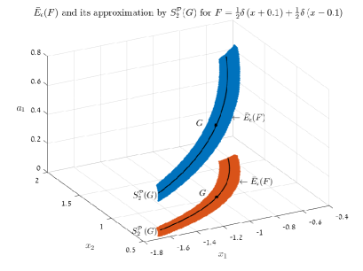
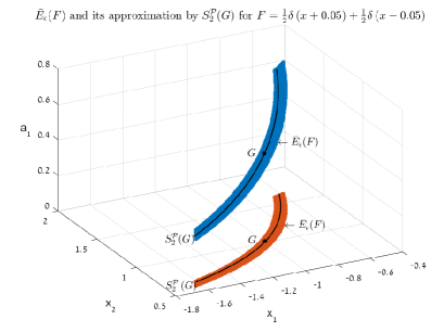
Figure 1: The projections of the error set $\bar{E}_{\epsilon}(F)$ and a section of the Prony curve $S^{\cal P}_{2}(G)$, for $h=0.1$ and $\epsilon=h^{3}$.

Figure 2: The error set $\bar{E}_{\epsilon}(F)$ and a section of $S^{\cal P}_{2}(G)$ for $h=0.05$ and $\epsilon=h^{3}$. Note the convergence of $\bar{E}_{\epsilon}(F)$ into $S^{\cal P}_{2}(G)$.

7.4 Applying quantitative Inverse Function Theorem

In order to apply this theorem, we have to make explicit assumptions on the separation of the nodes $X$ of the signal $G$, and on the size of its amplitudes $A$:

Assume that the nodes $x_{1},\ldots,x_{d}$ of a signal $G\in\bar{{\cal P}}_{d}$ belong to the interval $I=[-1,1]$, and for a certain $\eta$ with $0<\eta\leq\frac{2}{d-1}$, $d>1$, the distance between the neighboring nodes $x_{j},x_{j+1},\ j=1,\ldots,d-1,$ is at least $\eta$. We also assume that for certain $m,M$ with $0<m<M$, the amplitudes $a_{1},\ldots,a_{d}$ satisfy $m\leq|a_{j}|\leq M,\ j=1,\ldots,d$. We call such signals $(\eta,m,M)$-regular.

We want to show that for an $(\eta,m,M)$-regular signal $G\in\bar{\cal P}_{d}$ the moment coordinates $m_{0}(G^{\prime})-m_{0}(G),\ldots,m_{2d-1}(G^{\prime})-m_{2d-1}(G)$ indeed form a coordinate system near $G$, which agrees with the standard coordinates $A,\bar{X}$ on $\bar{\cal P}_{d}$.

Definition 7.2

For $G$ a regular signal as above, and $G^{\prime}$ denoting signals near $G$, the moment coordinates are the functions $f_{k}(G^{\prime})=m_{k}(G^{\prime})-m_{k}(G),\;k=0,...,2d-1$. The moment metric $d(G^{\prime},G^{\prime\prime})$ on $\bar{\cal P}_{d}$ is defined through the moment coordinates as

$$d(G^{\prime},G^{\prime\prime})={\rm max\,}_{k=0}^{2d-1}|m_{k}(G^{\prime\prime})-m_{k}(G^{\prime})|.$$

For any $\nu\in{\cal M}_{d}$ and $R>0$ denote by $Q_{R}(\nu)\subset{\cal M}_{d}$ the cube of radius $R$

$$Q_{R}(\nu)=\{\nu^{\prime}=(\nu^{\prime}_{0},\ldots,\nu^{\prime}_{2d-1})\in{\cal M}_{d},\ |\nu^{\prime}_{k}-\nu_{k}|\leq R,\ k=0,1,\ldots,2d-1\}.$$ (7.3)

Theorem 7.2

Let $G\in\bar{\cal P}_{d}$ be an $(\eta,m,M)$ regular signal and $\nu=PM(G)$. Then there are constants $R,C_{1},C_{2}$, depending only on $d,\eta,m,M$, given explicitly in [1], such that:

1. The inverse mapping $PM^{-1}$ exists on $Q_{R}(\nu)$ and provides a diffeomorphism of $Q_{R}(\nu)$ to $\Omega_{R}(G)=PM^{-1}(Q_{R}(\nu))$.

2. The moment metric $d(G^{\prime},G^{\prime\prime})$ is bi-Lipschitz equivalent on $\Omega_{R}(G)$ to the maximum metric $||G^{\prime\prime}-G^{\prime}||$ in $\bar{\cal{P}}_{d}$:

   $$C_{1}\ d(G^{\prime},G^{\prime\prime})\leq||G^{\prime\prime}-G^{\prime}||\leq C_{2}\ d(G^{\prime},G^{\prime\prime}).$$

Assume now that the measurement error $\epsilon\leq Rh^{\prime 2d-1}$, with $h^{\prime}=\frac{h}{1+|\kappa|}$ as in Theorem 7.1. Then

$$PM(\bar{E}_{\epsilon}(F))\subseteq PM(\Pi_{\epsilon,\frac{1}{h^{\prime}}}(G))\subset Q_{R}(PM(G)).$$

Combing Theorems 7.1 and 7.2 we obtain that the error set $\bar{E}_{\epsilon}(F)$ is a “deformed” paralelipiped in $\bar{{\cal P}}_{d}$ as illustrated in figures 2 and 2 above.

We use regular signals $G$ as above, to model signals with a “regular cluster”: For $F\in{\cal P}_{d}$ with $h=h(F)$ and $\kappa=\kappa(F)$, we say that $F$ forms an $(h,\kappa,\eta,m,M)$-regular cluster if $G=\Psi_{\kappa,h}(F)$ is an $(\eta,m,M)$-regular signal.

The next theorem shows that the $\epsilon$-error set is tightly concentrated around the Prony varieties.

Definition 7.3

For each $0\leq q\leq 2d-1$ denote by $S^{{\cal P}}_{q,\epsilon,\alpha}(G)$ the part of the Prony variety $S^{{\cal P}}_{q}(G),$ consisting of all signals $G^{\prime}\in S^{{\cal P}}_{q}(G)$ with

$$|m_{k}(G^{\prime})-m_{k}(G)|\leq\epsilon\alpha^{k},\ k=q+1,\ldots,2d-1.$$

Theorem 7.3

Let $F\in{\cal P}_{d}$ form an $(h,\kappa,\eta,m,M)$-regular cluster and let $G=\Psi_{\kappa,h}(F)$ be the model signal for $F$. Set $h^{\prime}=\frac{h}{1+|\kappa|}$. Then for any $\epsilon\leq Rh^{\prime 2d-1}$, the error set $\bar{E}_{\epsilon}(F)$ is contained within the $\Delta_{q}$-neighborhood of the part of the Prony variety $S^{{\cal P}}_{q,\epsilon,\frac{1}{h^{\prime}}}(G)$, for

$$\Delta_{q}=C_{2}\left(\frac{1}{h^{\prime}}\right)^{q}\epsilon.$$

The constants $R,C_{2}$ are defined in Theorem 7.2 above.

7.5 Worst case reconstruction error

We now present lower and upper bounds, of the same order, for the worst case reconstruction error $\rho(F,\epsilon),$ defined, as above, by:

$$\rho(F,\epsilon)={\rm max\,}_{F^{\prime}\in E_{\epsilon}(F)}||F^{\prime}-F||.$$

We state separate bounds for $\rho_{A}(F,\epsilon)$ and $\rho_{X}(F,\epsilon)$ - the worst case errors in reconstruction of the amplitudes $A=(a_{1},\ldots,a_{d})$ and of the nodes $X=(x_{1},\dots,x_{d})$ of $F$:

$$\rho_{A}(F,\epsilon)={\rm max\,}_{F^{\prime}\in E_{\epsilon}(F)}||A^{\prime}-A||,\ \rho_{X}(F,\epsilon)={\rm max\,}_{F^{\prime}\in E_{\epsilon}(F)}||X^{\prime}-X||.$$

Theorem 7.4

[Upper bound] Let $F\in{\cal P}_{d}$ form an $(h,\kappa,\eta,m,M)$-regular cluster. Then for each positive $\epsilon\leq\left(\frac{h}{1+|\kappa|}\right)^{2d-1}R$ the following bounds for the worst case reconstruction errors are valid:

$$\rho(F,\epsilon),\;\rho_{A}(F,\epsilon)\leq C_{2}\left(\frac{1+|\kappa|}{h}\right)^{2d-1}\epsilon,\hskip 20.00003pt\rho_{X}(F,\epsilon)\leq C_{2}h\left(\frac{1+|\kappa|}{h}\right)^{2d-1}\epsilon,$$

where $C_{2},R$ are the constants defined in Theorem 7.2.

Theorem 7.5

[Lower bound] Let $F\in{\cal P}$ form an $(h,\kappa,\eta,m,M)$-regular cluster then:

1. For each positive $\epsilon\leq C_{3}h^{2d-1}$ we have the following lower bound on the worst case reconstruction error of the nodes of $F$

   $$K_{1}\epsilon\left(\frac{1}{h}\right)^{2d-2}\leq\rho_{X}(F,\epsilon).$$

2. For each positive $\epsilon\leq C_{4}h^{2d-1}$ we have the following lower bound on the worst case reconstruction error of $F$ and of the amplitudes of $F$

   $$K_{2}\epsilon\left(\frac{1}{h}\right)^{2d-1}\leq\rho(F,\epsilon),\;\rho_{A}(F,\epsilon).$$

Above, $K_{1},K_{2},C_{3},C_{4}$ are constants not depending on $h$ given explicitly in [1].

The lower and upper bounds given above are a special case of a more general result. In [1] (Theorem 4.4) it is shown that the Prony variety $S^{\cal P}_{q}(G)$ can be reconstructed from the moment measurements $\mu^{\prime}\in{\cal M}_{d}$ with improved accuracy of order $\epsilon h^{-q}$.

8 Prony Scenarios

We keep the assumption that the nodes of our signal $F$ form a regular cluster of a size $h\ll 1$. By Theorem 7.3, the signal Prony curve $S^{\cal P}(\mu)$ approximates the error set $E_{\epsilon}(F)$ with the accuracy of order $\epsilon h^{-2d+2}$. Note that the accuracy of point solution is of order $\epsilon h^{-2d+1}$. Thus, the Prony curve $S^{\cal P}(\mu)$ provides a rather accurate prediction of the possible behavior of all the noisy reconstructions of $F$.

In an actual solution procedure, the “true” Prony curve $S^{\cal P}(\mu)$ is not known. But from the noisy measurements $\mu^{\prime}=(m^{\prime}_{0},\ldots,m^{\prime}_{2d-1})$ we can reconstruct the Prony curve $S^{\cal P}(\mu^{\prime})$. This curve, by Theorem 4.4 in [1], approximates the “true curve” $S^{\cal P}(\mu)$ with an accuracy of the same (improved) order of $\epsilon h^{-2d+2}$, with which $S^{\cal P}(\mu)$ approximates $E_{\epsilon}(F)$. Therefore, we can consider this known curve $S^{\cal P}(\mu^{\prime})$ as a prediction (or a “scenario”) for all the noisy reconstructions of $F$.

Moreover, if we neglect possible errors of order $\epsilon h^{-2d+2}$, we can restrict the search of the optimal Prony solution (by any method, in particular, via statistical estimations) to the curve $S^{\cal P}(\mu^{\prime})$.

We do not try to give here a rigorous definition of the “Prony scenario”. Informally, this is a collection of data on the Prony curve $S^{\cal P}(\mu^{\prime})$, which is necessary in order to find the optimal Prony solution on this curve, taking into account the available a priori constraints. Certainly we need an accurate description of the behavior of the nodes $x_{j}$ and the amplitudes $a_{j}$ along $S^{\cal P}(\mu^{\prime})$ (or, better, along the polynomial Prony curve $S^{\cal V}(\mu^{\prime})\subset{\cal V}_{d}$), including description of the intersection of $S^{\cal V}(\mu^{\prime})$ with the hyperbolicity set $H_{d}$.

Some general results in this direction were obtained in [29]:

Theorem 8.1

([29]) Assume that the matrix $M_{d}(\mu^{\prime})$ is non-degenerate. Then in each case where the nodes $x_{i},x_{j}$ collide on $S^{\cal P}(\mu^{\prime})$, the amplitudes $a_{i}$ and $a_{j}$ tend to infinity.

Theorem 8.2

([29]) Assume that the matrix $M_{d}(\mu^{\prime})$ is non-degenerate, as well as its upper-left $(d-1)\times(d-1)$ minor. Then on each unbounded component of $S^{{\cal P},X}(\mu^{\prime})$, for the coordinate $m_{2d-1}$ on $S^{\cal P}(\mu^{\prime})$ tending to infinity, exactly one node ($x_{1}$ or $x_{d}$) tends to infinity, while the rest of the nodes remain bounded.

The polynomial Prony curves $S^{\cal V}$ can be considered as polynomials pencils. Some important results on the behavior of the real roots in polynomial pencils are provided in [15, 35]. The result of [44] describing the behavior of roots in smooth 1-parametric families of polynomials may also be relevant. These results naturally enter the framework of the Prony scenarios, and in [29] we provide their more detailed treatment.

9 Some open questions

We would like to specify some open problems in the line of this paper. Mostly they concern the structure of the Prony varieties in the areas not covered by the inverse function theorem (Theorem 7.2 above).

1. Description of the global topology and geometry of the Prony varieties. In the topological study of the Vandermonde varieties in [4, 32] certain natural Morse functions were used. Can this method be extended to the Prony varieties?

On the other hand, an explicit parametrization of the Prony varieties, described in Section 5 above, reduces the problem to the study of the intersections of the affine subspaces in the polynomial space with the hyperbolic set $H_{d}$ (which is motivated also by the considerations in Section 8 above). This study looks natural also from the point of view of Singularity Theory.

2. Understanding connections between the Prony and the Vandermonde varieties. The last are the fibers of a natural projection of the corresponding Prony varieties to the amplitudes. Is this projection regular? What topological information on the Prony varieties can be obtained from the known properties of the Vandermonde ones? Can information available on the Prony varieties (in particular, their explicit parametrization, see Section 5 above) be useful in study of the Vandermonde ones?

3. Behavior of the nodes $x_{1},\ldots,x_{d}$ on the Prony varieties $S^{\cal P}_{q}(\mu)\subset{\cal P}_{d}$ near the collision singularities. It would be important to describe an accurate asymptotic behavior of the distances between the colliding nodes as we approach the collision point. This question can be split into two: investigation of the intersection of the affine varieties $S^{\cal V}_{q}(\mu)\subset{\cal V}_{d}$ with the boundary of the hyperbolic set $H_{d}$, and investigation of the behavior of the root mapping $RM$ near the boundary of $H_{d}$.

Already the case of the Prony curves is important and non-trivial.

4. Behavior of the amplitudes $a_{1},\ldots,a_{d}$ on the Prony varieties $S^{\cal P}_{q}(\mu)\subset{\cal P}_{d}$ near the collision singularities. In the case of the Prony curve, i.e. $q=2d-2$, Theorem 8.1 above gives conditions under which these amplitudes necessarily tend to infinity. It would be important to describe the accurate asymptotic behavior of the amplitudes as we approach the collision point. We expect that this question can be treated via methods from the classical Moment theory, combined with the techniques of “bases of finite differences” developed in [11, 53]. Also here the case of the Prony curves is important.

5. Extending the description of the Prony varieties, and of the error amplification patterns, to multi-cluster nodes configurations. This is a natural setting in robust inversion of the Prony system. Generalized Prony methods as well as other reconstruction methods typically reduce each cluster to a single node, thus forming a “reduced Prony system”. It is important to estimate the accuracy of such an approximation (see [30] for some steps in this direction).

Because of the role of the Prony varieties in the analysis of the error amplification patterns, a natural question is: To what extent do the Prony varieties of the reduced Prony system approximate the varieties of the “true” multi-cluster system?

References

- [1] A. Akinshin, D. Batenkov, G. Goldman, and Y. Yomdin. Error amplification in solving Prony system with near-colliding nodes. arXiv preprint arXiv:1701.04058, 2017.
- [2] A. Akinshin, D. Batenkov, and Y. Yomdin. Accuracy of spike-train Fourier reconstruction for colliding nodes. In 2015 International Conference on Sampling Theory and Applications (SampTA), pages 617–621. IEEE, 2015.
- [3] A. Akinshin, G. Goldman, V. Golubyatnikov, and Y. Yomdin. Accuracy of reconstruction of spike-trains with two near-colliding nodes. In Proc. Complex Analysis and Dynamical Systems VII, volume 699, pages 1–17. The AMS and Bar-Ilan University, 2015.
- [4] V. I. Arnol’d. Hyperbolic polynomials and Vandermonde mappings. Functional Analysis and Its Applications, 20(2):125–127, 1986.
- [5] J. R. Auton, M. L. Van Blaricum, et al. Investigation of procedures for automatic resonance extraction from noisy transient electromagnetics data. In AFWL Math. Note 79. General Research Corp Santa Barbara, Calif, 1981.
- [6] D. Batenkov. Complete algebraic reconstruction of piecewise-smooth functions from Fourier data. Mathematics of Computation, 84(295):2329–2350, 2015.
- [7] D. Batenkov. Stability and super-resolution of generalized spike recovery. Applied and Computational Harmonic Analysis, 2016.
- [8] D. Batenkov. Accurate solution of near-colliding Prony systems via decimation and homotopy continuation. Theoretical Computer Science, 2017.
- [9] D. Batenkov and Y. Yomdin. Algebraic Fourier reconstruction of piecewise smooth functions. Mathematics of Computation, 81(277):277–318, 2012.
- [10] D. Batenkov and Y. Yomdin. On the accuracy of solving confluent Prony systems. SIAM Journal on Applied Mathematics, 73(1):134–154, 2013.
- [11] D. Batenkov and Y. Yomdin. Geometry and singularities of the Prony mapping. Journal of Singularities, 10:1–25, 2014.
- [12] A. Bernardi, J. Brachat, and B. Mourrain. A comparison of different notions of ranks of symmetric tensors. Linear Algebra and its Applications, 460:205–230, 2014.
- [13] L. Birbrair and M. P. Denkowski. Medial axis and singularities. The Journal of Geometric Analysis, 27(3):2339–2380, 2017.
- [14] T. Blu, P.-L. Dragotti, M. Vetterli, P. Marziliano, and L. Coulot. Sparse sampling of signal innovations. IEEE Signal Processing Magazine, 25(2):31–40, 2008.
- [15] J. Borcea and B. Shapiro. Classifying real polynomial pencils. International mathematics research notices, 2004(69):3689–3708, 2004.
- [16] L. N. Bryzgalova. The maximum functions of a family of functions that depend on parameters (Russian). Funktsional’nyi Analiz i ego Prilozheniya, 12(1):66–67, 1978.
- [17] E. J. Candès and C. Fernandez-Granda. Super-resolution from noisy data. Journal of Fourier Analysis and Applications, 19(6):1229–1254, 2013.
- [18] E. J. Candès and C. Fernandez-Granda. Towards a mathematical theory of super-resolution. Communications on Pure and Applied Mathematics, 67(6):906–956, 2014.
- [19] W. Cheng. Generalized characteristics and singularities of solutions to Hamilton-Jacobi equations. The international conference on Singularity Theory and Dynamical Systems. In memory of John Mather, TSIMF, Sanya, China, 2017.
- [20] C. Ciliberto. Geometric aspects of polynomial interpolation in more variables and of Waring’s problem. In European Congress of Mathematics, Vol. I (Barcelona, 2000), volume 201 of Progress in Mathematics, pages 289–316. Birkhäuser/Springer, Basel, Switzerland, 2001.
- [21] P. Comon, G. Golub, L.-H. Lim, and B. Mourrain. Symmetric tensors and symmetric tensor rank. SIAM Journal on Matrix Analysis and Applications, 30(3):1254–1279, 2008.
- [22] L. Demanet and N. Nguyen. The recoverability limit for superresolution via sparsity. arXiv preprint arXiv:1502.01385, 2015.
- [23] D. K. Dimitrov and V. P. Kostov. Distances between critical points and midpoints of zeros of hyperbolic polynomials. Bulletin des sciences mathematiques, 134(2):196–206, 2010.
- [24] D. L. Donoho. Superresolution via sparsity constraints. SIAM journal on mathematical analysis, 23(5):1309–1331, 1992.
- [25] Y. C. Eldar. Sampling theory: Beyond bandlimited systems. Cambridge University Press, 2015.
- [26] C. Fernandez-Granda. Super-resolution of point sources via convex programming. Information and Inference: A Journal of the IMA, 5(3):251–303, 2016.
- [27] R. Fröberg and B. Shapiro. On Vandermonde varieties. Mathematica Scandinavica, 119(1):73–91, 2016.
- [28] T. Fukuda and S. Janeczko. Singularities of implicit differential systems and their integrability. Banach Center Publications, 65:23–47, 2004.
- [29] G. Goldman, Y. Salman, and Y. Yomdin. Prony scenarios and error amplification in a noisy spike-train reconstruction. arXiv preprint arXiv:1803.01685, 2018.
- [30] G. Goldman and Y. Yomdin. On algebraic properties of low rank approximations of Prony systems. arXiv preprint arXiv:1803.09243, 2018.
- [31] V. V. Goryunov. Semi-simplicial resolutions and homology of images and discriminants of mappings. Proceedings of the London Mathematical Society, 3(2):363–385, 1995.
- [32] V. P. Kostov. On the geometric properties of Vandermonde’s mapping and on the problem of moments. Proceedings of the Royal Society of Edinburgh Section A: Mathematics, 112(3-4):203–211, 1989.
- [33] V. P. Kostov. Root configurations for hyperbolic polynomials of degree 3, 4, and 5. Functional Analysis and its Applications, 36(4):311–314, 2002.
- [34] V. P. Kostov. Topics on hyperbolic polynomials in one variable. Panoramas et Synthèses-Société Mathématique de France, (33), 2011.
- [35] K. Kurdyka and L. Paunescu. Nuij type pencils of hyperbolic polynomials. Canadian mathematical bulletin, 60(3):561–570, 2017.
- [36] S. Lundqvist, A. Oneto, B. Reznick, and B. Shapiro. On generic and maximal k-ranks of binary forms. arXiv preprint arXiv:1711.05014, 2017.
- [37] W. L. Marar and D. Mond. Multiple point schemes for corank 1 maps. Journal of the London Mathematical Society, 2(3):553–567, 1989.
- [38] J. N. Mather. Solutions of generic linear equations. In Dynamical Systems, pages 185–193. Elsevier, 1973.
- [39] V. Matov. The topological classification of germs of the maximum and minimax functions of a family of functions in general position. Russian Mathematical Surveys, 37(4):127–128, 1982.
- [40] R. Miranda. Linear systems of plane curves. Notices AMS, 46(2):192–202, 1999.
- [41] V. I. Morgenshtern and E. J. Candès. Super-resolution of positive sources: the discrete setup. SIAM Journal on Imaging Sciences, 9(1):412–444, 2016.
- [42] E. M. Nikishin and V. N. Sorokin. Rational approximations and orthogonality. Amer Mathematical Society, 1991.
- [43] J. J. Nuño-Ballesteros. A Lê-Greuel type formula for the image Milnor number. The international conference on Singularity Theory and Dynamical Systems. In memory of John Mather, TSIMF, Sanya, China, 2017.
- [44] A. Parusinski and A. Rainer. Regularity of roots of polynomials. Annali della Scuola Normale Superiore di Pisa. Classe di Scienze. Serie V, 16(2):481–517, 2016.
- [45] T. Peter and G. Plonka. A generalized Prony method for reconstruction of sparse sums of eigenfunctions of linear operators. Inverse Problems, 29(2), 2013.
- [46] G. Plonka and M. Tasche. Prony methods for recovery of structured functions. GAMM-Mitteilungen, 37(2):239–258, 2014.
- [47] D. Potts and M. Tasche. Fast ESPRIT algorithms based on partial singular value decompositions. Applied Numerical Mathematics, 88:31–45, 2015.
- [48] R. Prony. Essai experimental et analytique etc. J. de l’Ecole Polytechnique, 1:24–76, 1795.
- [49] G. M. Reeve and V. M. Zakalyukin. Singularities of the minkowski set and affine equidistants for a curve and a surface. Topology and its Applications, 159(2):555–561, 2012.
- [50] Y. Yomdin. On the local structure of a generic central set. Compositio Math, 43(2):225–238, 1981.
- [51] Y. Yomdin. On functions representable as a supremum of a family of smooth functions. SIAM Journal on Mathematical Analysis, 14(2):239–246, 1983.
- [52] Y. Yomdin. On functions representable as a supremum of a family of smooth functions II. SIAM Journal on Mathematical Analysis, 17(4):961–969, 1986.
- [53] Y. Yomdin. Singularities in algebraic data acquisition. In Real and Complex singularities, volume 380 of London Mathematical Society Lecture Note Series, pages 378–396. Cambridge University Press, Cambridge, 2010.
- [54] V. M. Zakalyukin. Singularities of convex hulls of smooth manifolds. Functional Analysis and Its Applications, 11(3):225–227, 1977.
- [55] R. Zhang and G. Plonka. Optimal approximation with exponential sums by maximum likelihood modification of Prony’s method. Universität Göttingen, Institut für Numerische und Angewandte Mathematik, preprint, 2017.