Finding Faster Configurations using FLASH

Abstract

Finding good configurations of a software system is often challenging since the number of configuration options can be large. Software engineers often make poor choices about configuration or, even worse, they usually use a sub-optimal configuration in production, which leads to inadequate performance. To assist engineers in finding the better configuration, this article introduces Flash, a sequential model-based method that sequentially explores the configuration space by reflecting on the configurations evaluated so far to determine the next best configuration to explore. Flash scales up to software systems that defeat the prior state-of-the-art model-based methods in this area. Flash runs much faster than existing methods and can solve both single-objective and multi-objective optimization problems. The central insight of this article is to use the prior knowledge of the configuration space (gained from prior runs) to choose the next promising configuration. This strategy reduces the effort (i.e., number of measurements) required to find the better configuration. We evaluate Flash using 30 scenarios based on 7 software systems to demonstrate that Flash saves effort in 100% and 80% of cases in single-objective and multi-objective problems respectively by up to several orders of magnitude compared to state-of-the-art techniques.

1 Introduction

Most software systems available today are configurable; that is, they can be easily adjusted to achieve a wide range of functional and non-functional (e.g., energy or performance) properties. Once a configuration space becomes large, it becomes difficult for humans to keep track of the interactions between the configuration options. Section 2 of this article offers more details on many of the problems seen with software configuration. In summary:

• Many software systems have poorly chosen defaults [1, 2]. Hence, it is useful to seek better configurations.

• Understanding the configuration space of software systems with large configuration spaces is challenging [3].

• Exploring more than just a handful of configurations is usually infeasible due to long benchmarking time [4].

This article describes Flash, a novel way to find better configurations for a software system (for a given workload). Flash is a sequential model-based method (SMBO) [5, 6, 7] that reflects on the evidence (configurations) retrieved at some point to select the estimated best configuration to measure next. This way, Flash uses fewer evaluations to find better configurations compared to more expensive prior work [8, 9, 10, 11, 12].

Prior work in this area primarily used two strategies. Firstly, researchers used machine learning to model the configuration space. The model is built sequentially, where new configurations are sampled randomly, and the quality or accuracy of the model is measured using a holdout set. The size of the holdout set in some cases could be up to 20% of the configuration space [11] and needs to be evaluated (i.e., measured) before even the model is fully built. This strategy makes these methods not suitable in a practical setting since the generated holdout set can be (very) expensive. Secondly, the sequential model-based techniques used in prior work relied on Gaussian Process Models (GPM) to reflect on the configurations explored (or evaluated) so far [13]. However, GPMs do not scale well for software systems with more than a dozen configuration options [14].

The key idea of Flash is to build a performance model that is just accurate enough for differentiating better configurations from the rest of the configuration space. Tolerating the inaccuracy of the model is useful to reduce the cost (measured in terms of the number of configurations evaluated) and the time required to find the better configuration. To increase the scalability of methods using GPM, Flash replaces the GPMs with a fast and scalable decision tree learner.

Family	Software Systems	Objectives	#Config Options	Configuration Options	Description	Abbr	# Configu- rations	Prev Used
Stream Processing Systems	wc-c1-3d	Throughput	3	max spout, spliters, counters	Word Count is executed by varying 3 configurations of Apache Storm on cluster C1	SS-A1	1343	[15]
		Latency				SS-A2
	wc-c3-3d	Throughput	3	max spout, spliters, counters	Word Count is executed by varying 3 configurations of Apache Storm on cluster C3	SS-C1	1512
		Latency				SS-C2
	wc+wc-c4-3d	Throughput	3	max spout, spliters, counters	Word Count is executed, collocated with Word Count task, by varying 3 configurations of Apache Storm on cluster C3	SS-D1	195
		Latency				SS-D2
	wc-c4-3d	Throughput	3	max spout, spliters, counters	Word Count is executed by varying 3 configurations of Apache Storm on cluster C4	SS-E1	756
		Latency				SS-E2
	wc+rs-c4-3d	Throughput	3	max spout, spliters, counters	Word Count is executed, collocated with Rolling Sort task, by varying 3 configurations of Apache Storm on cluster C4	SS-F1	196
		Latency				SS-F2
	wc+sol-c4-3d	Throughput	3	max spout, spliters, counters	Word Count is executed, collocated with SOL task, by varying 3 configurations of Apache Storm on cluster C3	SS-G1	195
		Latency				SS-G2
	wc-5d-c5	Throughput	5	spouts, splitters, counters,buffer-size, heap	Word Count is executed by varying 5 configurations of Apache Storm on cluster C3	SS-I1	1080
		Latency				SS-I2
	rs-6d-c3	Throughput	6	spouts, max spout, sorters, emitfreq, chunksize, message size	Rolling Sort is executed by varying 6 configurations of Apache Storm on cluster C3	SS-J1	3839
		Latency				SS-J2
	wc-6d-c1	Throughput	6	spouts, max spout, sorters,emitfreq, chunksize,,message size	Word Count is executed by varying 6 configurations of Apache Storm on cluster C1	SS-K1	2880
		Latency				SS-K2
FPGA	sort-256	Area	3	Not specified	The design space consists of 206 different hardware implementations of a sorting network for 256 inputs	SS-B1	206	[13]
		Throughput				SS-B2
	noc-CM-log	Energy	4	Not specified	The design space consists of 259 different implementations of a tree-based network-on-chip,targeting application specific circuits (ASICs) and,multi-processor system-on-chip designs	SS-H1	259
		Runtime				SS-H2
Compiler	llvm	Performance	11	time passes, gvn, instcombine,inline, … , ipsccp, iv users, licm	The design space consists of 1023 different compiler settings for the LLVM compiler framework. Each setting is specified by d = 11 binary flags.	SS-L1	1023
		Memory Footprint				SS-L2
Mesh Solver	Trimesh	# Iteration	13	F, smoother, colorGS,relaxParameter, V, Jac- obi, line, zebraLine, cycle, alpha, beta,preSmo- othing, postSmoothing	Configuration space of Trimesh, a library to manipulate triangle meshes	SS-M1	239,260	[16]
		Time to Solutions				SS-M2
Video Encoder	X264-DB	PSNR	17	no mbtree, no asm, no cabac, no scenecut,…, keyint, crf, scenecut, seek, ipratio	Configuration space of X-264 a video encoder	SS-N1	53,662
		Energy				SS-N2
Seismic Analysis Code	SaC	Compile-Exit	59	extrema, enabledOptimizations, disabledOptimizations,ls, dcr, cf, lir, inl, lur, wlur, …maxae, initmheap, initwheap	Configuration space of SaC	SS-O1	65,424
		Compile-Read				SS-O2

Table I: Configuration problems explored in this article. The abbreviations of the systems (Abbr) are sorted in the order of the number of configuration options of the system. The column #Config Options represent the number of configuration options of the software system and #Configurations represents the total number of configurations of the system. See http://tiny.cc/flash_systems/ for more details.

The novel contributions of the article are:

• We show that Flash can solve single-objective performance configuration optimization problems using an order of magnitude fewer measurements than the state-of-the-art (Section 7.1). This is a critical feature because, as discussed in Section 2, it can be very slow to sample multiple properties of modern software systems, when each such sample requires (say) to compile and benchmark the corresponding software system.

• We empower Flash to multi-objective performance configuration optimization problems.

• We show that Flash overcomes the shortcomings of prior work and achieves similar performance and scalability, with greatly reduced runtimes (Section 7.2).

• Background material, a replication package, all measurement data, and the open-source version of Flash are available at supplementary website (http://tiny.cc/flashrepo/).

The rest of the article is structured as follows: Section 2 motivates this work. Section 3 describes the problem formulation and the theory behind SMBO. Section 4 describes prior work in software performance configuration optimization, followed by the core algorithm of Flash in Section 5. In Section 6, we present our research questions along with experimental settings used to answer them. Prior work in this area addresses a single-objective problem with the only exception of ePAL [13]. Hence, we evaluate Flash separately for single-objective and multi-objective performance configuration optimization problems. In Section 7, we apply Flash on single-objective performance configuration optimization and multi-objective performance configuration optimization. The article ends with a discussion on various aspects of Flash, and finally, we conclude along with a discussion of future work.

2 Performance configuration optimization for Software

This section motivates our research by reviewing the numerous problems associated with software configuration.

Many researchers report that modern software systems come with a daunting number of configuration options. For example, the number of configuration options in Apache (a popular web server) increased from 150 to more than 550 configuration options within 16 years [3]. Van Aken et al. [1] also reports a similar trend. They indicate that, in over 15 years, the number of configuration options of Postgres and MySQL increased by a factor of three and six, respectively. This is troubling since Xu et al. [3] report that developers tend to ignore over 80% of configuration options, which leaves considerable optimization potential untapped and induces major economic cost [3]. For illustration, Figure I offer examples of the kinds of configuration options seen in software systems.

Another problem with configurable systems is the issue of poorly chosen default configurations. Often, it is assumed that software architects provide useful default configurations of their systems. This assumption can be very misleading. Van Aken et al. report that the default MySQL configurations in 2016 assume that it will be installed on a machine that has 160MB of RAM (which, at that time, was incorrect by, at least, an order of magnitude) [1]. Herodotou et al. [2] show how standard settings for text mining applications in Hadoop result in worst-case execution times. In the same vein, Jamshidi et al. [15] reports for text mining applications on Apache Storm, the throughput achieved using the worst configuration is 480 times slower than the throughput achieved by the best configuration.

Yet another problem is that exploring benchmark sets for different configurations is very slow. Wang et al. [17] comments on the problems of evolving a test suite for software if every candidate solution requires a time-consuming execution of the entire system: such test suite generation can take weeks of execution time. Zuluaga et al. [18] report on the cost of analysis for software/hardware co-design: “synthesis of only one design can take hours or even days”.

The challenges of having numerous configuration options are just not limited to software systems. The problem to find an good set of configuration options is pervasive and faced in numerous other sub-domains of computer science and beyond. In software engineering, software product lines–where the objective is to find a product which (say) reduces cost and defects [19, 20]—have been widely studied. The problem of configuration optimization is present in domains, such as machine learning, cloud computing, and software security.

The area of hyper-parameter optimization (a.k.a. parameter tuning) is very similar to the performance configuration optimization problem studied in this article. Instead of optimizing the performance of a software system, the hyper-parameter method tries to optimize the performance of a machine learner. Hyper-parameter optimization is an active area of research in various flavors of machine learning. For example, Bergstra and Bengiol [21] showed how random search could be used for hyper-parameter optimization of high dimensional spaces. Recently, there has been much interest in hyper-parameter optimization applied to the area of software analytics [22, 23, 24, 25, 26].

Another area of application for performance configuration optimization is cloud computing. With the advent of big data, long-running analytics jobs are commonplace. Since different analytic jobs have diverse behaviors and resource requirements, choosing the correct virtual machine type in a cloud environment has become critical. This problem has received considerable interest, and we argue, this is another useful application of performance configuration optimization — that is, optimize the performance of a system while minimizing cost [5, 27, 28, 29, 30].

As a sideeffect of the wide-spread adoption of cloud computing, the security of the instances or virtual machines (VMs) has become a daunting task. In particular, optimized security settings are not identical in every setup. They depend on characteristics of the setup, on the ways an application is used or on other applications running on the same system. The problem of finding security setting for a VM is similar to performance configuration optimization [31, 32, 33, 34, 35]. Among numerous other problems which are similar to performance configuration optimization, the problem of how to maximize conversions on landing pages or click-through rates on search-engine result pages [36, 37, 4] has gathered interest.

The rest of this article discusses how Flash addresses configuration problems (using the case studies of Figure I).

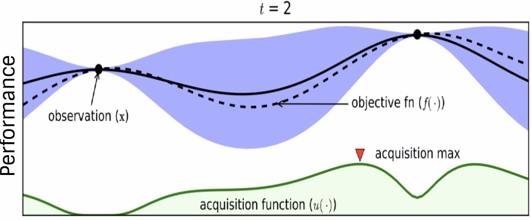
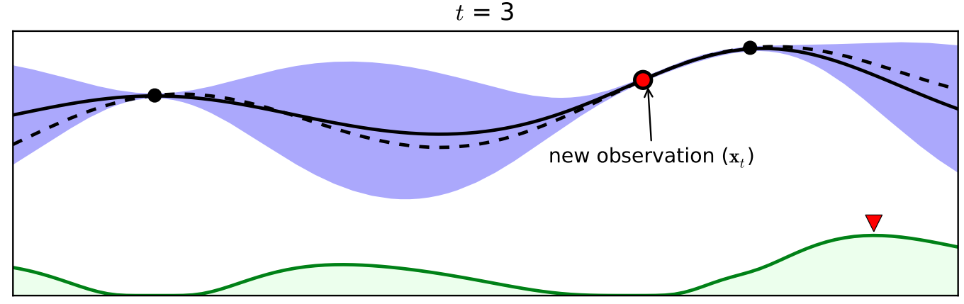
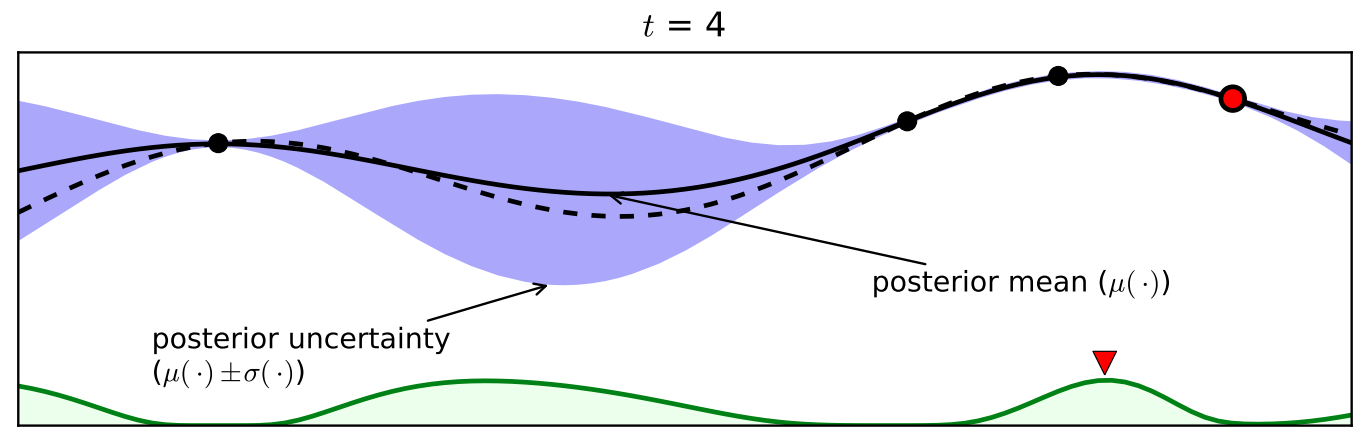
Figure 1: An example of Sequential Model-based method’s working process from [7]. The figures show a Gaussian process model (GPM) of an objective function over four iterations of sampled values. Green shaded plots represent acquisition function. The value of the acquisition function is high where the GPM predicts larger objective and where the prediction uncertainty (confidence) is high such points (configurations in our case) is sampled first. Note that the area on the far left is never sampled even when it has high uncertainty (low confidence) associated.

3 Theory

The following theoretical notes define the framework used throughout the article.

3.1 What are Configurable Software Systems?

A configurable software system has a set $X$ of configurations $x\in X$. Let $x_{i}$ represent the ith configuration of a software system. $x_{i,j}$ represent the jth configuration option of the configuration $x_{i}$. In general, $x_{i,j}$ indicates either an (i) integer variable or a (ii) Boolean variable. The configuration space ($X$) represents all the valid configurations of a software system. The configurations are also referred to as independent variables. Each configuration ($x_{i}$), where $1\leq i\leq|X|$, has one (single-objective) or many (multi-objective) corresponding performance measures $y_{i,k}\in Y$, where $y_{i,k}$ indicates the $1\leq kth\leq m$ objective associated with a configuration $x_{i}$. The performance measure is also referred to as dependent variable. For multi-objective problems, there are multiple dependent variables. We denote the performance measures ($y\in Y$) associated with a given configuration by $(y_{i,1},..y_{i,m})=f(x_{i})$, in multi-objective setting $y_{i}$ is a vector, where: $f:X\mapsto Y$ is a function which maps $X\in R^{n}$ to $Y\in R^{m}$. In a practical setting, whenever we try to obtain the performance measure corresponding to a certain configuration, it requires actually executing a benchmark run with that configuration. In our setting, evaluation of a configuration (or using $f$) is expensive and is referred to as a measurement. The cost or measurement is defined as the number of times $f$ is used to map a configuration $x_{i}\in X$ to $Y$. In our setting, the cost of an optimization technique is the total number of measurements required to find the better solution.

In the following, we will explore two different kinds of configuration optimization: single-objective and multiple objective. In single-objective performance configuration optimization, we consider the problem of finding a good configuration ($x^{*}$) such that $f(x^{*})$ is less than other configurations in $X$. Our objective is to find $x^{*}$ while minimizing the number of measurements.

$$f(x^{*})\leq f(x),\leavevmode\nobreak\ \leavevmode\nobreak\ \leavevmode\nobreak\ \forall x\in{X\setminus x^{*}}$$ (1)

That is, our goal is to find the better configuration of a system with least cost or measurements as possible when compared to prior work.

In multi-objective performance configuration optimization, we consider the problem of finding a configuration ($x^{*}$) that is better than other configurations in the configuration space of $X$ while minimizing the number of measurements. Unlike, the single-objective configuration optimization problem, where one solution can be the best (optimal) solution (except multiple configurations have the same performance measure), in multi-objective configuration optimization there may be no best solution (best in all objectives). Rather there may be a set of solutions that are equivalent to each other. Hence, to declare that one solution is better than another, all objectives must be polled separately. Given two vectors of configurations $x_{1},x_{2}$ with associated objectives $y_{1},y_{2}$, then $x_{1}$ is binary dominant ($\succ$) over $x_{2}$ when:

$$\begin{gathered}y_{1,p}\leq y_{2,p}\forall p\in\{1,2,...,m\}\leavevmode\nobreak\ \leavevmode\nobreak\ \text{and}\\ y_{1,q}<y_{2,q}\leavevmode\nobreak\ \leavevmode\nobreak\ \text{for at least one index}\leavevmode\nobreak\ \leavevmode\nobreak\ q\in\{1,2,...,m\}\end{gathered}$$ (2)

where $y\in Y$ are the performance measures. We refer to binary dominant configurations as better configurations. For the multi-objective configuration optimization problem, our goal is to find a set of better configurations of a given software system using fewer measurements compared to prior work.

3.2 Sequential Model-based Optimization

Sequential Model-based Optimization (SMBO) is a useful strategy to find extremes of an unknown objective (or performance) function which is expensive (both in terms of cost and time) to evaluate. In literature, a certain variant of SMBO is also called Bayesian optimization. SMBO is efficient because of its ability to incorporate prior belief as already measured solutions (or configurations), to help direct further sampling. Here, the prior represents the already known areas of the search (or performance optimization) problem. The prior can be used to estimate the rest of the points (or unevaluated configurations). Once we have evaluated one (or many) points based on the prior, we can define the posterior. The posterior captures our updated belief in the objective function. This step is performed by using a machine learning model, also called surrogate model.

The concept of SMBO is simple stated:

• Given what we know about the problem…

• … what should we do next?

The “given what we know about the problem” part is achieved by using a machine learning model whereas “what should we do next” is performed by an acquisition function. Such acquisition function automatically adjusts the exploration (“should we sample in uncertain parts of the search space) and exploitation (“should we stick to what is already known”) behavior of the method.

This can also be explained as follows. Firstly, few points (or configurations) are (say) randomly selected and measured. These points along with their performance measurements are used to build a model (prior). Secondly, this model is then used to estimate or predict the performance measurements of other unevaluated points (or configurations).This can be used by an acquisition function to select the configurations to measure next. This process continues till a predefined stopping criterion (budget) is reached.

Much of the prior research in configuration optimization of software systems can be characterized as an exploration of different acquisition functions. These acquisition function (or sampling heuristics) were used to satisfy two requirements: (i) use a ‘reasonable’ number of configurations (along with corresponding measurements) and (ii) the selected configurations should incorporate the relevant interactions—how different configuration options influence the performance measure [38]. In a nutshell, the intuition behind such functions is that it is not necessary to try all configuration options—for pragmatic reasons. Rather, it is only necessary to try a small representative configurations—which incorporates the influences of various configuration options. Randomized functions select random items [8, 9]. Other, more intricate, acquisition functions first cluster the data then sample only a subset of examples within each cluster [10]. But the more intricate the acquisition function, the longer it takes to execute—particularly for software with very many configurations. For example, recent studies with a new state-of-the-art acquisition function show that such approaches are limited to models with less than a dozen decisions (i.e. configuration options) [13].

As an example of an acquisition function, consider Figure 1. It illustrates a time series of a typical run of SMBO. The bold black line represents the actual performance function ($f$—which is unknown in our setting) and the dotted black line represents the estimated objective function (in the language of SMBO, this is the prior). The purple regions represent the configuration or uncertainty of estimation in a region—the thicker that region, the higher the uncertainty.

The green line in that figure represents the acquisition function. The optimization starts with two points (t=2). At each iteration, the acquisition function is maximized to determine where to sample next. The acquisition function is a user-defined strategy, which takes into account the estimated performance measures (mean and variance) associated with each configuration.. The chosen sample (or configuration) maximizes the acquisition function (argmax). This process terminates when a predefined stopping condition is reached which is related to the budget associated with the optimization process.

Gaussian Process Models (GPM) is often the surrogate model of choice in the machine learning literature. GPM is a probabilistic regression model which instead of returning a scalar ($f(x)$) returns the mean and variance associated with $x$. There are various acquisition functions to choose from: (1) Maximum Mean, (2) Maximum Upper Interval, (3) Maximum Probability of Improvement, (4) Maximum Variance, and (5) Maximum Expected Improvement.

Building GPMs can be very challenging since:

• GPMs can be very fragile, that is, very sensitive to the parameters of GPMs;

• GPMs do not scale to high dimensional data as well as a large dataset (software system with large configuration space) [39]. For example, in SE, the state-of-the-art in this area using GPMs for optimization was limited to models with around ten decisions  [14].

4 performance optimization of Configurable Software Systems

In this section, we discuss the model-based methods used in the prior work to find the better configurations of software systems.

4.1 Residual-based: “Build an Accurate Model”

In this section, we discuss the residual-based method for building performance models for software systems, which, in SMBO terminology, is an optimizer with a flat acquisition function, that is, all the points are equally likely to be selected (random sampling).

When the cost of collecting data (benchmarking time) is higher than the cost of building a performance model (surrogate model), it is imperative to minimize the number of measurements required for model building. A learning curve shows the relationship between the size of the training set and the accuracy of the model. In Figure 2, the horizontal axis represents the number of samples used to create the performance model, whereas the vertical axis represents the accuracy (measured in terms of MMRE—Mean Magnitude of Relative Error) of the model learned. Learning curves typically have a steep sloping portion early in the curve followed by a plateau late in the curve. The plateau occurs when adding data does not improve the accuracy of the model. As engineers, we would like to stop sampling as soon as the learning curve starts to flatten. Two types of residual-based methods have been introduced in Sarkar et al. namely progressive and projective sampling.

(1) Progressive Sampling uses an iterative sampling strategy to inform the process of building the performance model. It starts by sampling a small set of configurations and their corresponding performance measures to build a model and validating the model using a holdout set. Configurations are iteratively sampled and used to construct the performance model until the performance model achieves a specified accuracy (measured in terms of MMRE). The sampling process terminates when a predefined threshold is reached. One of the shortcomings of progressive sampling is that the resulting performance model achieves an acceptable accuracy only after a large number of iterations, which implies high modeling cost. There is no way to determine the cost of modeling until the performance model is already built, which defeats its purpose, as there is a risk of over-shooting the modeling budget and still not obtaining an accurate model.
(2) Projective sampling addresses this problem by approximating the learning curve using a minimal set of initial configurations, thus providing the stakeholders with an estimate of the modeling cost.

We use progressive sampling as a representative because projective sampling adds only a sample estimation technique to the progressive sampling and does not add anything to the sampling itself.

The residual-based method discussed here considers only performance configuration optimization scenarios with a single-objective. In the residual-based method, the correctness of the performance model built is measured using error measures such as MMRE:

$$\mathit{MMRE}=\frac{\mid\mathit{f(x)}-\mathit{y}\mid}{\mathit{y}}\cdot 100$$ (3)

For further details, please refer to Sarkar et. al [9].

Figure 2: The relationship between the accuracy and the number of samples used to train the performance model of the running Word Count application on Apache Storm. Note that the accuracy does not improve substantially after 20 sample configurations.

Figure 3 is a generic algorithm that defines the process of progressive sampling. Progressive sampling starts by clearly defining the data used in the training set (called training pool) and used for testing the quality of the surrogate model (in terms of residual-based measures) called holdout set. The training pool is the set from which the configurations would be selected (randomly, in this case) and then tested against the holdout set. At each iteration, a (set of) data instance(s) of the training pool is added to the training set (Line 9). Once the data instances are selected from the training pool, they are evaluated, which in our setting means measuring the performance of the selected configuration (Line 12). The configurations and the associated performance scores are used to build the performance model (Line 14). The model is validated using the testing set, then the accuracy is computed. In our setting, we assume that the measure is accuracy (higher is better). Once the accuracy score is calculated, it is compared with the accuracy score obtained before adding the new set of configurations to the training set. If the accuracy of the model (with more data) does not improve the accuracy when compared to the previous iteration (lesser data), then life is lost. This termination criterion is widely used in the field of Evolutionary Algorithms to determine the degree of convergence [40].

⬇

1 # Progressive Sampling

2 def progressive(training, holdout, lives=3):

3 # For stopping criterion

4 last_score = -1

5 independent_vals = list()

6 dependent_vals = list()

7 for count in range(1, len(training)):

8 # Add one configuration to the training set

9 independent_vals += training[count]

10 # Measure the performance value for the newly

11 # added configuration

12 dependent_vals += measure(training_set[count])

13 # Build model

14 model = build_model(independent_vals, dependent_vals)

15 # Test Model

16 perf_score = test_model(model, holdout, measure(holdout))

17 # If current accuracy score is not better than

18 # the previous accuracy score, then loose life

19 if perf_score <= last_score:

20 lives -= 1

21 last_score = perf_score

22 # If all lives are lost, exit loop

23 if lives == 0: break

24 return model

Figure 3: Python code of progressive sampling, a residual-based method.

4.2 Rank-based: “Build a Rank-preserving Model”

As an alternative to the residual-based method, a rank-based method has recently been proposed [11]. The rank-based method is similar to residual-based method in that it has a flat acquisition function, which resembles random sampling. Like the residual-based method, the rank-based method discussed here also considers only performance configuration optimizations with a single-objective. For further details, please refer to Nair et. al [11].

⬇

1# rank-based method

2def rank_based(training, holdout, lives=3):

3 last_score = -1

4 independent_vals = list()

5 dependent_vals = list()

6 for count in range(1, len(training)):

7 # Add one configuration to the training set

8 independent_vals += training[count]

9 # Measure the performance value for the newly

10 # added configuration

11 dependent_vals += measure(training_set[count])

12 # Build model

13 model = build_model(independent_vals, dependent_vals)

14 # Predicted performance values

15 predicted_performance = model(holdout)

16 # Compare the ranks of the actual performance

17 # scores to ranks of predicted performance scores

18 actual_ranks = ranks(measure(holdout))

19 predicted_ranks = ranks(predicted_performance)

20 mean_RD = RD(actual_ranks, predicted_ranks)

21 # If current rank difference is not better than

22 # the previous rank difference, then loose life

23 if mean_rank_difference <= last_rank_difference:

24 lives -= 1

25 last_rank_difference = mean_RD

26 # If all lives are lost, exit loop

27 if lives == 0: break

28 return model

Figure 4: Python code of rank-based method.

In a nutshell, instead of using residual measures of errors, as described in Equation 3, which depend on residuals ($r=y-f(x)$), it uses a rank-based measure. While training the performance model ($f(x)$), the configuration space is iteratively sampled (from the training pool) to train the performance model. Once the model is trained, the accuracy of the model is measured by sorting the values of $y=f(x)$ from ‘small’ to ‘large’, that is:

$$f(x_{1})\leq f(x_{2})\leq f(x_{3})\leq...\leq f(x_{n}).$$ (4)

The predicted rank order is then compared to the actual rank order. The accuracy is calculated using the mean rank difference ($\mu RD$):

$$\mathit{\mu RD}=\frac{1}{n}\cdot{{\sum}}_{i=1}^{n}\Big{\lvert}rank(y_{i})-rank(f(x_{i}))\Big{\rvert}$$ (5)

This measure simply counts how many of the pairs in the test data have been ordered incorrectly by the performance model $f(x)$ and measures the average of magnitude of the ranking difference.

In Figure 4, we list a generic algorithm for the rank-based method. Sampling starts by selecting samples randomly from the training pool and by adding them to the training set (Line 8). Then, the collected sample configurations are evaluated (Line 11). The configurations and the associated performance measure are used to build a performance model (Line 13). The generated model (CART, in our case) is used to predict the performance measure of the configurations in the testing pool (Line 16). Since the performance value of the holdout set is already measured, hence known, the ranks of the actual performance measures, and predicted performance measure are calculated. (Lines 18–19). The actual and predicted performance measure is then used to calculate the rank difference using Equation 5. If the rank difference ($\mu RD$) of the model (with more data) does not decrease when compared to the previous generation (lesser data), then a life is lost (Lines 23–24). When all lives are expired, sampling terminates (Line 27).

⬇

1 # ePAL Multi-objective SMBO

2 def ePAL(all_configs, $\varepsilon$, size = 20):

3 # Add |\textit{size}| number of randomly selected

4 # configurations to training data

5 train = random.sample(all_configs, size)

6 # Measure the performance value for sampled training data

7 train = [ measure(x) for x in train ]

8 # Remove the measured configurations from configuration space

9 all_configs = all_configs $\setminus$ train

10 # Till all the configurations in all_configs has been either sampled or discarded

11 while len(all_configs) > 0:

12 # Build GPM

13 model = GPM(train)

14 # Get prediction and corresponding confidence intervals

15 # associated with each configuration in all_configs

16 $\mu$, $\sigma$ = model.predict(all_configs)

17 # Only keep configurations discard based on uncertainty

18 all_configs = all_configs - discard(all_configs,$\mu$, $\sigma$, $\varepsilon$)

19 # Find and measure another point based on acquisition function.

20 new_point = measure(acquisition_function(all_configs, $\mu$, $\sigma$))

21 # Add new_point to train

22 train += new_point

23 return train

Figure 5: Python code of ePAL, a multi-objective SMBO.

4.3 ePAL: “Traditional SMBO”

Unlike the residual-based and rank-based methods, epsilon Pareto Active Learning (ePAL) reflects on the evaluated configurations (and corresponding performance measures) to decide the next best configuration to measure using Maximum Variance (predictive uncertainty) as an acquisition function. ePAL incrementally updates a model (GPM) representing a generalization of all samples (or configurations) seen so far. The model can be used to decide the next most promising configuration to evaluate. This ability to avoid unnecessary measurement (by just exploring a model) is very useful in the cases where each measurement can take days to weeks.

In Figure 5, we list a generic algorithm for ePAL. ePAL starts by selecting samples randomly from the configuration space (all_configs) and by adding them to the training set (Line 5). The collected sample configurations are then evaluated (Line 7). The configurations and the associated performance values are used to build a performance model (Line 13). The generated model (GPM, in this case) is used to predict the performance values of the configurations in the testing pool (Line 16). Note that the model returns both the value ($\mu$) as well as the associated confidence interval ($\sigma$). These predicted values are used to discard configurations, which have a high probability of being dominated by another point (Line 18). Domination is defined in Equation 2 . After configurations (which have a high probability of being dominated) have been discarded, a new configuration (new_point) is selected and measured (Line 20). The selected configuration new_point is the most uncertain in all_configs. Then, new_point is added to train, which is then used to build the model in the subsequent iteration (Line 22). When all the configuration in all_configs have been discarded (or evaluated and moved to train) the process terminates.

Note again, since ePAL is a traditional SMBO, it shares its shortcomings (refer to Section 3.2).

5 FLASH: A Fast Sequential Model-based Method

To overcome the shortcomings of the traditional SMBO, Flash makes certain design choices:

• Flash's acquisition function uses Maximum Mean. Maximum Mean returns the sample (configuration) with highest expected (performance) measure;

• GPM is replaced with CART [41], a fixed-point regression model. This is possible because the acquisition function requires only a single point value rather than the mean and the associated variance.

When used in a multi-objective optimization setting, Flash models each objective as a separate performance (CART) model. This is because the CART model can be trained for one performance measure or dependent value.

The basic idea of CART is as follows: CART recursively partitions the set of configurations (based on a configuration option) into smaller clusters until the performance of the configurations in the clusters are similar. Each split of the set of configurations is driven by a decision on the configuration option that would minimize the entropy or prediction error. These recursive clustering is represented as a binary decision tree. So, when we need to predict the performance of a new configuration not measured so far, we use the decision tree to find the cluster which is most similar to the new configuration.

Flash replaces the actual evaluation of all configurations (which can be a very slow process) with a surrogate evaluation, where the CART decision trees are used to guess the objective scores (which is a very fast process). Once guesses are made, then some select operator must be applied to remove less-than-satisfactory configurations. Inspired by the decomposition approach of MOEA/D [42], Flash uses the following stochastic Maximum Mean method, which we call Bazza.

For problems with $o$ objectives that we seek to maximize, Bazza returns the configuration that has outstandingly maximum objective values across $N$ random projections. Using the predictions for the $o$ objectives from the learned CART models, then Bazza executes as follows. Note that the first step (randomly assigning weights to goals) is a technique we burrow and adapt from the MOEA/D algorithm [42].

• $N$ vectors $V$ of length $m$ are generated and filled with random numbers of the range 0..1. This represents the various weight vectors. The idea is to decompose one problem into a set of $N$ sub-problems (uniformly spread $N$ weight vectors.

• Set $\mathit{max=0}$ and $\mathit{best=nil}$.

• For each configuration $x_{i}$

  • Guess its performance scores $y_{i,j}$ using the predictions from the CART models.

  • Compute its mean weight as follows:

    $$\centering mean_{i}=\frac{1}{N}\sum_{n}^{N}\sum_{j}^{{\mathit{m}}}\left(V_{n,j}\cdot x_{i,j}\right)\@add@centering$$ (6)

  • If $\mathit{mean}>\mathit{max}$, then $\mathit{max:=mean}$ and $\mathit{best}:=x_{i}$.

• Return $\mathit{best}$.

In summary, given a set of $V$ weight vectors of length $m$, Bazza finds the vector that scores best across $N$ different weighted sums, each of which is computed with random weight vectors.

⬇

1def FLASH(uneval_configs, fitness, size, budget):

2 # Add |size| number of randomly selected configurations to training data.

3 # All the randomly selected configurations are measured

4 eval_configs = [measure(x) for x in sample(uneval_configs, size)]

5 # Remove the evaluations configuration from data

6 uneval_configs.remove(eval_configs)

7 # Till all the lives has been lost

8 while budget > 0:

9 # build one CART model per objective

10 for o in objectives: model[o] = CART(eval_configs)

11 # Find and measure another point based on acquisition function

12 acquired_point = measure(acquisition_fn(uneval_configs, model))

13 eval_configs += acquired_point # Add acquired point

14 uneval_config -= acquired_point # Remove acquired point

15 # Stopping Criteria

16 budget -= 1

17 return best

18

19def acquisition_fn(uneval_configs, model, no_directions=10):

20 # Predict the value of all the unevaluated configurations using model

21 predicted = model.predict(uneval_configs)

22 # If number of objectives is greater than 1 (In our setting len(objectives) = 2)

23 if len(objectives) > 1: # For multi-objective problems

24 return Bazza( predicted )

25 else: # For single-objective problems

26 return max(predicted)

Figure 6: Python code of Flash

The resulting algorithm is shown in Figure 6. Before initializing Flash, a user needs to define three parameters N, size, and budget (refer to Section 8.2 for a sensitivity analysis). Flash starts by randomly sampling a predefined number (size) of configurations from the configuration space and evaluate them (Line 4). The evaluated configurations are removed from the unevaluated pool of configurations (Line 6). The evaluated configurations and the corresponding performance measure/s are then used to build CART model/s (Line 10). This model (or models, in case of multi-objective problems) is then used by the acquisition function to determine the next point to measure (Line 13). The acquisition function accepts the model (or models) generated in Line 10 and the pool of unevaluated configurations (uneval_configs) to choose the next configuration to measure. The model is used to generate a prediction for the unevaluated configurations. For single-objective optimization problems, the next configuration to measure is the configuration with the highest predicted performance measure (Line 26). For multi-objective optimization problems, Bazza is applied. The configuration chosen by the acquisition function is evaluated and added to the evaluated pool of configurations (Line 12-13) and removed from the unevaluated pool (Line 14). Flash terminates once it runs out of budget (Line 8).

Note the advantages of this approach: SMBO is a widely used method [43] for many important tasks (cloud configuration [5], hyperparameter optimization [44]) so even a small improvement in this method would be significant for a large of number of domains Truly Flash includes many novel innovations. The following list shows the significant innovations of this work and the delta to prior research.
1. Evolutionary algorithms (EAs) have been used for optimizing black-box optimization [45]. Using Evolutionary Algorithms is relatively straightforward since it requires no domain knowledge to solve a problem.
Challenge: Evolutionary algorithms suffer from two problems. Firstly, there is the issue of the number of evaluations required for an EA. A standard EA experiment is 100 individuals mutated for 100+ generations [46]. This renders Evolutionary Algorithms unsuitable for our domain since individual evaluation can be very slow (requires re-running a benchmark suite). A second problem with EAs is the problem of slow convergence (i.e., the performance delta across these generations may be very slow and take a long time to stabilize  [47]). For this reason, research in this area in the last decade has explored non-EA methods for software configuration [16, 8, 9, 10, 11].
New approach:

• Here we explore SMBO for software configuration optimization.

• While SMBO is gaining some popularity in other domains [5, 48, 49], this article is the first reporting a successful application of SMBO to software configuration.

2. Prior work in this area used some surrogate model learned by data mining (e.g., with CART  [8, 9, 10]), possibly combined with random sampling. Such surrogates are useful for guiding the construction of better configuration models since they can be much faster to execute than (say) re-running a benchmark. Hence, an optimizer that uses such surrogates can terminate relatively quickly.
Challenge: One drawback with surrogate models is that they require a holdout set, against which the surrogate model (built iteratively) is evaluated. Interestingly, prior work does not discuss the cost of populating, which may require exploring up to 20% of the total configuration space [11].
New approach:

• We found that applying SMBO removes the need for this hold out. We build the model incrementally, thus the configurations (and their performance) sampled at a given point in time used to intelligently select the next data point to collect.

• This work is the first successful application of such incremental model construction (with no holdout sets) for software configuration.

3. Standard SMBO algorithms are a widely used method for finding good samples (as used in hyper-parameter optimization). Standard SMBO builds its models using a method called Gaussian Process Models. Due to internal complexities of some of its matrix operations, GPM can handle only a dozen configuration options (or less), while modern software may required many more configuration options.
Challenge: How can we scale SMBO to much larger configuration options?
New approach:

• One of the core innovations of this article is the use of CART (one CART per goal) for surrogate modeling. That is, we replace GPM with CART. GPM takes time O($M^{3}$) [50] while recursive bifurcating algorithms like CART are much faster (takes time O($MN^{2}$) to build its trees where M is the size of the training dataset and N is the number of attributes [51]). Furthermore, methods such as CART have been extensively studied, and very fast incremental versions are simple to implement—see Domingos et al. [52], which is to say that if CART ever gets slow, there are many alternatives, we could try that would readily speed it up.

• Theoretical complexity results aside, we demonstrate empirically that that our CART-based method scales much better than GPM. As of 2016, published state-of-the-art results [14] report that they were unable to use more than 10 attributes within a GPM. As of 2018, our own experiments confirm that GPM cannot scale to more than a dozen configuration options. As shown in Figures 10(a) and (b), Flash scales linearly in number of attributes to models that defeats SMBO. We regard FLASH's ability to scale linearly in number of attributes to be a major contribution of this article.

4. One advantages of SMBO algorithms such as GPM is that they identify region(s) of most variance within a model. Such regions represent zones of most uncertainty (and sampling there has greatest chance of most improving a model).
Challenge: If we are not using GPM, how can we find the best regions for future sampling?
New approach:

• Another core innovation is the Bazza algorithm. Bazza assumes that the greatest mean might contain the values that most extend to the desired maximal (or minimal) goals. Bazza finds that region in linear time (since it only has to track the most extreme values seen so far).

• Bazza is an important innovation since standard methods for finding the best candidates within a population of size M require time O($M^{2}$) [53]. But as shown in this article, our methods require only O(M).

5. The kernels used in Gaussian Process Model assume “smoothness” [50], or in other words, the configurations which are closer to each other have similar performance. In the case of software configuration, this assumption is highly unlikely since we know of many software options where a small change can lead to radically different software performance (e.g. switching from link lists to B-trees is a single change to one value of one configuration option—but that change can lead to dramatic speed ups in the software). Challenge: How to avoid GPM’s smoothness assumptions?
New approach:

• We use CART, a learner that recursively bifurcates training data into different regions. The important point here is that CART makes no assumption that neighboring regions have the same properties.

• Unlike prior work, our use of CART makes no limiting assumptions about the smoothness of the space.

6 Evaluation

6.1 Research Questions

In prior work, performance configuration optimization was conducted by sequentially sampling configurations to build models, both accurate (residual-based method) and inaccurate (rank-based method). Both methods divide the configuration space into (i) training pool, (ii) validation set, and (iii) holdout set. They sequentially select a configuration from the training pool and add it to the training set (which is a subset of the training pool). The configuration (along with the corresponding performance measure) is used to build a model. Both methods use a validation set to evaluate the quality of the model. The size of the validation set is based on an engineering judgment and expected to be a representative of the whole configuration space. Prior work [11] used 20% of the configuration space as holdout set, but did not consider the cost of using the validation set.

Our research questions are geared towards assessing the performance of Flash based on two aspects: (i) Effectiveness of the solution or the rank-difference between the best configuration found by Flash to the actual best configuration, and (ii) Effort (number of measurements) required to find the better configuration.

The above considerations lead to two research questions: RQ1: Can Flash find the better configuration?
Here, the better configurations found using Flash are compared to the ones identified in prior work, using the residual-based and rank-based method. The effectiveness of the methods is compared using rank-difference (Equation 7).

RQ2: How expensive is Flash (in terms of how many configurations must be measured)?
It is expensive to build (residual-based or rank-based) models since they require using a holdout set. Our goal is to demonstrate that Flash can find better configurations of a software system using fewer measurements.

To the best of knowledge, SMBO has never been used for multi-objective performance configuration optimization in software engineering. However, similar work has been done by Zuluaga et al. [13] in the machine learning community, where they introduced ePAL. We use ePAL as a state-of-the-art method to compare Flash.

We do not consider the work by Oh et al. [54], which uses true random sampling to find the better configurations. We do not compare Flash with Oh et al.'s method mainly for the following reason: Oh et al.'s work supports only Boolean configuration options, which limits its practical applicability. Flash, and the prior work considered in this article, do not have this limitation. Moreover, Oh's work is limited to single-objective problems. Since it does not build a performance model during the search process, it cannot be easily adapted to multi-objective problems. One may argue that running Oh et al.'s approach alternatively on different objectives (of a multi-objective problem) could lead to a set of solutions on the Pareto Front. However, this is not a proper alternative since these runs (on separate objectives) are independent of each other (i.e., they are run separately and cannot inform each other).

Since ePAL suffers from the shortcomings of traditional SMBO, our research questions are geared towards finding the estimated Pareto-optimal solutions (predicted Pareto Frontier ), which is closest to the true Pareto Frontier (which requires measuring all configurations) with least effort. We assess the performance of Flash by considering three aspects: (i) Effectiveness of the configurations between the Pareto Frontier and the ones approximated by an optimizer, and Effort evaluated in terms of (ii) number of measurements, and (iii) time to approximate the Pareto Frontier.

The above considerations lead to three research questions: RQ3: How effective is Flash for multi-objective performance configuration optimization?
The effectiveness of the solution or the difference between the predicted Pareto Frontier found by optimizers to the true Pareto Frontier,
RQ4: Can Flash be used to reduce the effort of multi-objective performance configuration optimization compared to ePAL?
Effort (number of measurements) required to estimate the Pareto Frontier which is closest to the true Pareto Frontier, and
RQ5 Does Flash save time for multi-objective performance configuration optimization compared to ePAL?
Since ePAL may take substantial time to find the approximate the Pareto Frontier, it is imperative to show that Flash can approximate the Pareto Frontier and converge faster.

Our goal is to minimize the effort (time and number of measurements) required to find an approximate Pareto Frontier as close to the actual Pareto Frontier as possible.

6.2 Case Studies

We evaluated Flash in two different types of problems namely: (1) single-objective optimization problems and (2) multi-objective optimization problems using 30 scenarios (15 scenarios in multi-objective settings) from 6 software systems. These systems are summarized in Table I. More details about the software systems are available at http://tiny.cc/flash_systems/.

We selected these software systems since they are widely used in the configuration and search-based SE literature [16, 8, 9, 10, 11, 54, 15, 13] as benchmark problems for this kind of optimization work. Furthermore, extensive documentation is available at the supplementary Web site for all these models.

6.3 Experimental Rig

6.3.1 Exploring RQ1, RQ2

For each subject system, we build a table of data, one row per valid configuration. We then run all configurations of all systems (that is, that are invoked by a benchmark) and recorded the performance scores. Note that, while answering the research questions, we ensure that we never test any prediction model on the data that we used to learn the model.

To answer our research questions, we split the datasets into training pool (40%), holdout set (20%), and validation pool (40%). The size of the holdout set is taken from prior work [11]. It is worth to note that this is a hyper-parameter and is set based on an engineering judgment. To perform a fair comparison while comparing Flash with prior work, the training pool and validation pool are merged for Flash experiments.

The experiment to find better configuration using the residual-based and rank-based methods is conducted in the following way:

• Randomize the order of rows in the training data

• Do

  • Select one configuration (by sampling with replacement) and add it to the training set

  • Determine the performance scores associated with the configuration. This corresponds to a table look up but would entail compiling or configuring and executing a system configuration in a practical setting.

  • Using the training set and the accuracy, build a performance model using CART.

  • Using the data from the testing pool, assess the accuracy either using MMRE (as described in Equation 3) or rank difference (as described in Equation 5).

• While the accuracy is greater or equal to the threshold determined by the practitioner (rank difference in the case of rank-based method and MMRE in the case of residual-based method).

Once the model is trained, it is tested on the data in the validation pool. Please note, the learner has not been trained on the validation pool. The experiment to find better configuration by Flash is conducted in the following way:

• Choose 80% of the data (at random)

• Randomize the order of rows in the training data

• Do

  • Select 30 configurations (by sampling with replacement) and add them to the training set

  • Determine the performance scores associated with the configurations. This corresponds to a table look up, but would entail compiling or configuring and executing a system configuration in a practical setting.

  • Using the training set, build a performance model using CART.

  • Using the CART model, find the configuration with best predicted performance.

  • Add the configuration with best predicted performance to the training set.

• While the stopping criterion (budget) is not met, continue adding configurations to the training set.

Once Flash has terminated, the configuration with the best performance is selected as the better configuration. Please note that unlike the methods proposed in prior work, there is no training and validation pool in Flash. It uses the whole space and returns the configuration with the best performance.

RQ1 relates the results found by Flash to ones of residual-based and rank-based methods. We use the absolute difference between the ranks of the configurations predicted to be the best configuration and the actual optimal configuration. We call this measure rank difference.

$$\begin{split}RD&=Big\lvert\mathrm{rank(actual_{best})}-\mathrm{rank(predicted_{best})}Big\rvert\\ \end{split}$$ (7)

Ranks are calculated by sorting the configurations based on their performance scores. The configuration with the minimum performance score, $\mathrm{rank(actual_{best})}$, is ranked 1 and the one with the highest score is ranked as $N$, where $N$ is the number of configurations.

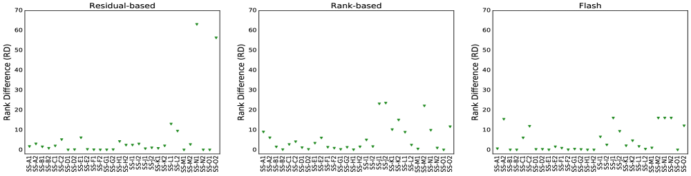
Figure 7: The rank difference of the prediction made by model built using the residual-based method, the rank-based methods, and Flash. Note that the y-axis of this chart rises to large values; e.g., SS-M has 239,260 possible configurations. Hence, the above charts could be summarized as follows: “the Flash is surprisingly accurate since the rank difference is usually close to 0% of the total number of possible configurations.”

6.3.2 Exploring RQ3, RQ4, and RQ5

Similar to RQ1 and RQ2, for each subject system, we build a table of data, one row per valid configuration. We then run all configurations of all systems and record the performance scores. To this table, we add two columns of measurements (one for each objective) obtained from measurements.

To measure effectiveness, we use quality indicators as advised by Wang et al. [55]. The quality indicators are:

• The Generational Distance (GD) [56] measures the closeness of the solutions from by the optimizers to the Pareto frontier that is, the actual set of non-dominated solutions.

• The Inverted Generational Distance (IGD) [57] is the mean distance from points on the true Pareto-optimal solutions to its nearest point in the predicted Pareto-optimal solutions returned by the optimizer.

Note that, for both measures, smaller values are better. Also, according to Coello et al. [57], IGD is a better measure of how well solutions of a method are spread across the space of all known solutions. A lower value of GD indicates that the predicted Pareto-optimal solutions have converged (or are near) to the actual Pareto-optimal solutions. However, it does not comment on the diversity (or spread) of the solutions. GD is useful while interpreting the results of RQ3 and RQ6, where we would notice that Flash has low GD values but relatively high IGD values.

To answer our research questions, we initialize ePAL and Flash with randomly selected configurations along with their corresponding performance scores. Since, ePAL does not have an explicit stopping criterion, we allow ePAL to run until completion. For Flash, we allowed a budget of 50 configurations. The value 50 was assigned by parameter tuning (from Section 8.2). The configurations evaluated during the execution of the three methods are then used to measure the quality measures (to compare methods). Note that we use two versions of ePAL: ePAL with $\epsilon=0.01$ (ePAL_0.01), and ePAL with $\epsilon=0.3$ (ePAL_0.3) . These ePAL versions represents two extremes of ePAL from the most cautious ($\epsilon=0.01$)—maximizing quality to most careless ($\epsilon=0.3$)—minimizing measurements. 

Other aspects of our experimental setting were designed in response to the specific features of the experiments. For example, all the residual-based, rank-based and Flash methods are implemented in Python. We use Zuluaga et al.'s implementation of ePAL, which was implemented in Matlab. Since we are comparing methods implemented in different languages, we measure “speed” in terms of the number of measurements (a language-independent feature) along with runtimes.

SS-A2
1	Rank-based	1.0	4.0
1	Residual-based	2.0	5.0
2	Flash	9.0	18.0

SS-C1
1	Residual-based	0.0	2.0
1	Rank-based	1.0	3.0
2	Flash	3.0	6.0

SS-C2
1	Rank-based	2.0	2.0
1	Residual-based	2.0	5.0
2	Flash	7.0	16.0

SS-E2
1	Residual-based	0.0	0.0
2	Rank-based	1.0	2.0
2	Flash	1.0	1.0

SS-J1
1	Residual-based	0.0	1.0
2	Flash	1.0	13.0
2	Rank-based	13.0	42.0

SS-J2
1	Residual-based	0.0	1.0
2	Rank-based	2.0	14.0
2	Flash	4.0	16.0

SS-K1
1	Residual-based	0.0	1.0
2	Rank-based	1.0	3.0
2	Flash	1.0	3.0

Figure 8: The median rank difference of 20 repeats. Median ranks are the rank difference as described in Equation 7, and IQR the difference between 75th percentile and 25th percentile found during multiple repeats. Lines with a dot in the middle (  ), show the median as a round dot within the IQR. All the results are sorted by the median rank difference: a lower median value is better. The left-hand column (Rank) ranks the various methods for example when comparing three techniques. For SS-A2, a rank-based method has a different rank since their median rank difference is statistically different. Please note, this chart only shows software systems where Flash is significantly worse than methods from prior work.

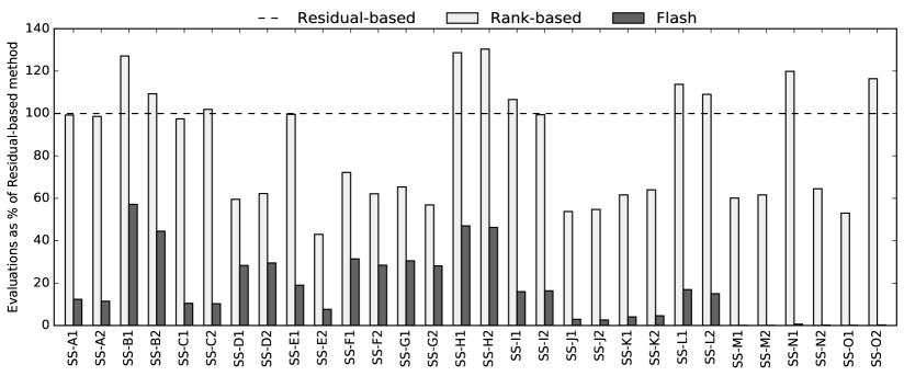
Figure 9: Measurements required to find better configurations with the residual-based method as the baseline.

7 Results

7.1 Single-objective Problems

RQ1: Can Flash find the better configuration?
Figure 7 shows the Rank Difference of the predictions using Flash, the rank-based method and the residual based method. The horizontal axis shows subject systems. The vertical axis shows the rank difference (Equation 7).

• The ideal result would be when all the points lie on the line y=0 or the horizontal axis, which means the method was able to find the better configurations for all subject systems or the rank difference between the predicted optimal solution and the actual optimal solution is 0.

• The sub-figures (left to right) represent the residual-based method, rank-based method, and Flash.

Overall, in Figure 7, we find that:

• All methods can find better configurations. For example, Flash for SS-J1 predicted the configuration whose performance score is ranked 20th in configuration space. That is good enough since Flash finds the 20th most performant configuration among 3072 configurations.

• The mean rank difference of the predicted optimal configuration is 6.082, 5.81, and 5.58  for residual-based, rank-based, and Flash.

So, the rank of the better configuration found by all the three methods is practically the same. To verify the similarity is statistically significant, we further studied the results using non-parametric tests Scott-Knott test recommended by Mittas and Angelis [58] and Arcuri & Briand [58].

Scott-Knott is a top-down clustering approach used to rank different treatments. If the approach finds an interesting division of the data, then some statistical test is applied to the two divisions to check if they are statistically significantly different. If so, Scott-Knott recurses into both halves. To apply Scott-Knott, we sorted a list of $l=20$ values of performance of different method found by different methods. Then, we split $l$ into sub-lists $m,n$ to maximize the expected value of differences in the observed performances before and after division. For example, for lists $l,m,n$ of size $ls,ms,ns$ where $l=m\cup n$:

$$E(\Delta)=\frac{ms}{ls}|m.\mu-l.\mu|^{2}+\frac{ns}{ls}|n.\mu-l.\mu|^{2}$$

We then apply a statistical hypothesis test $H$ to check if $m,n$ are significantly different (in our case, the conjunction of A12 and bootstrapping). If so, Scott-Knott recurses on the splits. In other words, we divide the data if both bootstrap sampling and effect size test agree that a division is statistically significant (with a confidence level of 99%) and not a small effect ($A12\geq 0.6$).

For a justification of the use of non-parametric bootstrapping, see Efron & Tibshirani [59, p220-223]. For a justification of the use of effect size tests, see Shepperd and MacDonell [60]; Kampenes [61]; and Kocaguenli et al. [62]. These researchers warn that, even if a hypothesis test declares two populations to be “significantly” different, then that result is misleading if the “effect size” is very small. Hence, to assess the performance differences we first must rule out small effects using A12.

In Figure 8, we show the Scott-Knott ranks for the three methods. The quartile charts show the Scott-Knott results for the subject systems, where Flash did not do as well as the other two methods. For example, the statistic test for SS-C2 shows that the rank difference of configurations found by Flash is statistically larger from the other methods. This is reasonably close, since the median rank of the configurations found by Flash is 7 of 1512 configurations, where for the other methods found configurations have a median rank of 2. As engineers, we feel that this is close because we can find the 7th best configuration using 34 measurements compared to 339 and 346 measurements used by other methods. Overall, our results indicate that: Flash can find better configurations, similar to the residual-based and the rank-based method, of a software system without using a holdout set.

RQ2: How expensive is Flash (in terms of how many configurations must be executed)?
To recommend Flash as a cheap method for performance optimization, it is important to demonstrate that it requires fewer measurements to find the better configurations. In our setting, the cost of finding the better configuration is quantified by number of measurements required (i.e., table lookup). Figure 9 shows our results. The vertical axis represents the ratio of the measurements of different methods are represented as the percentage of number of measurements required by residual-based method – since it uses the most measurements in 66% scenarios.

Overall, we see that Flash requires the least number of measurements to find better configurations. For example, in SS-E1, Flash requires 9% of the measurements when compared with the residual-based method and the rank-based method. There are few cases (SS-M1 to SS-O2) where Flash requires less than 1% of the residual-based method, which is because these systems have a large configuration space and the holdout set required by the residual-based method and the rank-based method (except Flash) uses 20% of the measurements. For performance configuration optimization, Flash is cheaper than the state-of-the-art method. In 57% of the software systems, Flash requires an order of magnitude fewer measurement compared to the residual-based method and rank-based method.

7.2 Multi-objective Optimization

RQ3: How effective is Flash for multi-objective performance configuration optimization?
Table II shows the results of a statistical analysis that compares the quality measures of the approximated Pareto-optimal solutions generated by Flash to those generated by ePAL.

• The rows of the table shows median numbers of 20 repeated runs over 15 different scenarios.

• The columns report the quality measures, generational distance (GD), and inverted generation distance (IGD). Recall smaller values of GD and IGD are better.

• ‘X’ denotes cases where a method did not terminate within a reasonable amount of time (10 hours).

• Bold-typed results are statistically better than the rest.

• The last row of the table (Win (%)) reports the percentage of times a method is significantly better than other methods overall software systems.

One way to get a quick summary of this table is to read the last row (Win(%)). This row is the percentage number of times a method was marked statistically better than the other methods. From Table II, we can observe that Flash outperforms variants of ePAL since Flash has the highest Win(%) in both quality measures. This is particularly true for scenarios with more than 10 configuration options, where ePAL failed to terminate while Flash always did.

We further notice that ePAL-0.01 has a higher win percentage than ePAL-0.3. This is not surprising since (as discussed in Section 6.3.2) ePAL-0.01 (optimized for quality) is more cautious than ePAL-0.3 (which is optimized for speed measured in terms of number of measurements). This can be regarded as a sanity check. It is interesting to note that Flash has impressive convergence score (lower GD scores)—it converges better for 93% of the systems, but not so remarkable in terms of the spread (lower IGD scores). However, the performance of Flash is similar to ePAL. It is also interesting that, for software systems where Flash was not statistically better, these are cases where the statistically better method always converged to the actual Pareto Frontier (with few exceptions).

Flash is effective for multi-objective performance configuration optimization. It also works in software systems with more than 10 configuration options whereas ePAL does not terminate in reasonable time.

Table II: Statistical comparisons of Flash and ePAL regarding the Performance measures are GD (Generational Distance), IGD (Inverted Generational Distance) and a number of measurements. For all measures, less is better; “X” denotes cases where methods did not terminate within a reasonable amount of time (10hrs). The numbers in bold represent statistically better runs than the rest. For example, for SS-G, GD of Flash is statistically better than of ePAL.

Software	GD			IGD			Evals
	epal_0.01	epal_0.3	Flash	epal_0.01	epal_0.3	Flash	epal_0.01	epal_0.3	Flash
SS-A	0.002	0.002	0	0.002	0.002	0	109.5	73.5	50
SS-B	0	0	0.005	0	0.003	0.001	84.5	20	50
SS-C	0.001	0.001	0.003	0.004	0.004	0	247	101	50
SS-D	0	0.004	0.014	0.002	0.007	0.009	119.5	67	50
SS-E	0.001	0.001	0.012	0.004	0.008	0.002	208	54.5	50
SS-F	0	0.016	0.008	0	0.006	0.016	138	71	50
SS-G	0	0	0.023	0.003	0.006	0.004	131	69	50
SS-H	0	0	0	0	0	0	52	28	50
SS-I	0.008	0.018	0	0.008	0.018	0	48	30	50
SS-J	0	0	0.002	0.002	0.002	0	186	30	50
SS-K	0.001	0.001	0.003	0.001	0.002	0.001	209	140	50
SS-L	0.01	0.028	0.006	0.007	0.008	0.009	68.5	35	50
SS-M	X	X	0	X	X	0	X	X	50
SS-N	X	X	0.065	X	X	0.015	X	X	50
SS-O	X	X	3.01E-07	X	X	3.20E-06	X	X	50
Win (%)	73	67	93	67	33	67	0	33	80

RQ4: Can Flash be used to reduce the effort of multi-objective performance configuration optimization compared to ePAL?
In the RQ4 section (right-hand side) of Table II, the number of measurements required by methods, ePAL, and Flash are shown. Rows show different software systems and columns shows the number of measurements associated with each method. The numbers highlighted in bold mark methods that are statistically better than the other. For example in SS-K, Flash uses statistically fewer samples than (variants of) ePAL.

From the table we observe:

• Flash uses fewer samples than ePAL_0.01. In 9 of 15 cases, ePAL_0.01 is, at least, two times better than Flash.

• (Variants of) ePAL does not terminate for SS-M, SS-N, and SS-O even after ten hours of execution—a pragmatic choice. The reason for this can be seen in Table I: these software systems have more than 10 configuration options and the GPMs used by ePAL does not scale beyond that number.

• The obvious feature of Table II is that Flash used fewer measurements in 12 of 15 software systems.

Flash requires fewer measurements than ePAL to approximate Pareto-optimal solutions. The number of evaluations used by Flash is less than (more careful) ePAL-0.01 for all the software systems and 12 of 15 software systems for (more careless) ePAL-0.3.

RQ5:Does Flash save time for multi-objective performance configuration optimization compared to ePAL?
Figure 10 compares the run times of ePAL with Flash. Please note that we use the author's version of ePAL in our experiments, which is implemented in Matlab. However, Flash was implemented in Python. Even though this may not be a fair comparison, for the sake of completeness, we report the run-times of the test. The sub-figure to the left shows how the run times vary with the number of configurations of the system. The x-axis represents the number of configurations (in log scale), while the y-axis represents the time taken to perform 20 repeats in seconds (in log scale), which means lower the better. The dotted lines in the figure, shows the cases where a method (in this case, ePAL) did not terminate. The sub-figure in the middle represents how the run-time varies with the number of configuration options. The x-axis represents the number of configuration options, and the y-axis represents the time taken for 20 repeats in seconds (in log scale), which means lower the better. The sub-figure to the right represent the performance gain achieved by Flash over (variants of) ePAL. The x-axis shows the software systems, and the Y-axis represents the gain ratio. Any bar higher than the line (y=1) represent cases where Flash is better than ePAL.

From the figure, we observe:

• From sub-figures left and middle, Flash is much faster than (variants of) ePAL except in 2 of 15 cases.

• The run times of ePAL increase exponentially with the number of configurations and configuration options, similar to the trend reported in the literature.

• (Variants of) ePAL does not terminate for cases with large numbers of configurations and configuration options, whereas Flash always terminates an order of magnitude faster than ePAL. This effect is magnified in case of a scenarios with large configuration space.

Overall our results indicate: Flash saves time and is faster than (variants of) ePAL in 13 of 15 cases. Furthermore, Flash is an order of magnitudes faster than ePAL in 5 of 15 software systems. In other 2 out of 15 cases, the Flash 's runtimes are similar to (variants of) ePAL.

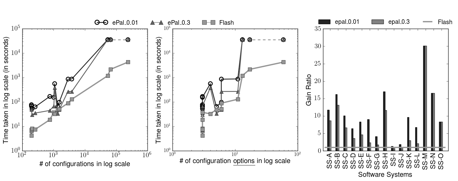
Figure 10: The time required to find better solutions using ePAL and Flash (sum of 20 repeats). Note that the axis's of the first two figures (left, and center) are in log scale. The time required for Flash compared to (variants of) ePAL is much lower (with an exception on 2 of 15 software systems). The dashed line in the figure (left and middle) represents cases where ePAL did not terminate within a reasonable time (10 hours). In the right-hand figure, we show the performance gain (wrt. to time) achieved by using Flash. All the bars above the dashed line (y=1) performs worse than Flash.

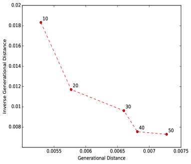
Figure 11: The trade-off between the number of starting samples (exploration) and number of steps to converge (exploitation). The ideal point in these trade-off curves is (0,0), which mean the algorithm has perfect convergence ($GD=0$) and perfect diversity ($IGD=0$). The trade-off curve for multi-objective performance configuration optimization is shown with budget of 50 evaluations.

8 Discussion

8.1 Why CART is used as the surrogate model?

Decision Trees are a very simple way to learn rules from a set of examples and can be viewed as a tool for the analysis of a large dataset. The reason why we chose CART is two-fold. Firstly, it is shown to be scalable and there is a growing interest to find new ways to speed up the decision tree learning process [51]. Secondly, a decision tree can describe with the tree structure the dependence between the decisions and the objectives, which is useful for induction and comprehensibility. These are the primary reasons for choosing decision-trees to replace Gaussian Process as the surrogate model for Flash.

8.2 What is the trade-off between the starting size and budget of Flash?

There are two main parameters of Flash which require being set very carefully. In our setting, the parameters are size and budget. The parameter size controls the exploration capabilities of Flash whereas parameter budget controls the exploitation capabilities. In Figure 11, we show the trade-off between generational distance and inverted generational distance by varying parameters size and budget. The markers in Figure 11 are annotated with the starting size of Flash. The trade-off characterizes the relationship between two conflicting objectives, for example in Figure 11, point (10) achieves high convergence (low GD value) but low diversity (high IGD value). Note, that the curves are an aggregate of the trade-off curves for all the software systems. From the figure 11 we observe that: The number of initial samples (size in Figure 6) determines the diversity of the solution. With ten initial samples the algorithm converges (lowest GD values) but lowest diversity (high IGD values). However, with 50 initial samples (random sampling) Flash achieves highest diversity (low IGD values) but lowest convergence (high GD values). We choose the starting size of 30 because it achieves a good trade-off between convergence and diversity. These values were used in the experiments in section 7.2.

8.3 Can rules learned by CART guide the search?

Currently, Flash does not explicitly reflect on the Decision Tree to select the next sample (or configuration). But, rules learned by Decision Tree can be used to guide the process of search. Though we have not tested this approach, a Decision Tree can be used to learn about importance of various configuration options which can be then used to recursively prune the configuration space, similar to the approach of Oh et al. [54]. We hypothesize that this would make Flash more scalable and be used to much larger models. We leave this for future work.

8.4 What are the shortcomings of Flash?

Flash suffers from the following shortcomings.

• Parallelization: Flash like all sequential model-based approaches completes evaluating a configuration before evaluating a new one. However, in practice, this feature can lead to really long runtimes. A possible extension might be to evaluate multiple configurations in parallel. This has not been considered in this version of Flash and is something we leave for the future work.

• Non-stationary: Flash assumes that the benchmark or the load in the system is stationary. Hence, there is no inherent mechanism in Flash which would adapt itself based on the change in workload. This non-stationary nature of the problem is a significant assumption and currently not addressed in this paper. Addressing this aspect may include an ensemble-based approach where a new model is built at a specified time interval. The importance of the model is defined by a time-dependent weight decay of the model, that is, older the model, the lower its significance (weight).

• Cost Sensitivity: Flash also assumes that the cost of evaluating all the configurations are same. However, in practice, this is not true. For example, the wall clock time of running a specific benchmark on a software system with and without caching can be substantially different. In practice, stakeholders may demand to find a good configuration within a specified time limit (instead of the number of configurations measured). We leave this for future work.

• Cold Start: Flash randomly selects the initial configurations to evaluate, which can affect its effectiveness. One of the way to reduce the impact of randomness its to select the initial points based on domain knowledge or use transfer learning from similar software systems that have been optimized in the past, to select the initial configurations of Flash.

9 Threats to Validity

Reliability refers to the consistency of the results obtained from the research. For example, how well can independent researchers reproduce the study? To increase external reliability, we took care to either define our algorithms or use implementations from the public domain (SciKitLearn) [63]. All code used in this work are available online .

Validity refers to the extent to which a piece of research investigates what the researcher purports to investigate [64]. Internal validity concerns with whether the differences found in the treatments can be ascribed to the treatments under study.

For the case-studies relating to configuration control, we cannot measure all possible configurations in a reasonable time. Hence, we sampled only a few hundred configurations to compare the prediction to actual values. We are aware that this evaluation leaves room for outliers and that measurement bias can cause false interpretations [65]. We also limit our attention to predicting PF for a given workload; we did not vary benchmarks.

Internal bias originates from the stochastic nature of multi-objective optimization algorithms. The evolutionary process required many random operations, same as the Flash was introduced in this article. To mitigate these threats, we repeated our experiments for 20 runs and reported the median of the indicators. We also employed statistical tests to check the significance of the achieved results.

It is challenging to find the representatives sample test cases to covers all kinds of software systems. We just selected six most common types of software system to discuss the Flash basing on them. In the future, we also need to explore more types of SBSE problems for other domains such as process planning, next release planning. We aimed to increase external validity by choosing case-studies from different domains.

10 Conclusion

This article proposes a sequential model-based method called Flash, an approach for finding better configurations while minimizing the number of measurements. To the best of our knowledge, this is the first time a sequential model-based method is used to solve the problem of performance configuration optimization. Flash sequentially gains knowledge about the configuration space like traditional SMBO. Flash is different from the traditional SMBOs because of the choice of the surrogate model (CART) and the acquisition function (the stochastic Maximum-Mean Bazza function). We have demonstrated the effectiveness of Flash on single-objective and multi-objective problems using 30 scenarios from 7 software systems.

For a single-objective setting, we experimentally demonstrate that Flash can locate the better configuration of 30 different scenarios for seven software systems, accurately compared to the state-of-the-art approaches while removing the need for a holdout dataset, hence saving measurement costs. In 57% of the scenarios, Flash can find the better configuration by using an order of magnitude fewer solutions than other state-of-the-art approaches.

For multi-objective setting, we show how Flash can overcome the shortcomings of traditional SMBO (ePAL) while being as effective as ePAL as well as being scalable to software systems with higher number (greater than 10) of configuration options (where ePAL does not terminate in a reasonable time-frame).

Regarding future work, the two directions for this research are i) test on different case studies and ii) further improve the scalability of Flash. To conclude, we urge the SE community to learn from communities which tackle similar problems. This article experiments with ideas from fields of machine learning, SBSE, and software analytics to create Flash, which is a fast, scalable and effective optimizer. We hope this article inspires other researchers to look further afield than their home discipline.

11 Acknowledgement

Apel's work has been supported by the German Research Foundation (AP 206/6, AP 206/7, and AP 206/11).

References

- [1] Dana Van Aken, Andrew Pavlo, Geoffrey J Gordon, and Bohan Zhang. Automatic database management system tuning through large-scale machine learning. In International Conference on Management of Data. ACM, 2017.
- [2] Herodotos Herodotou, Harold Lim, Gang Luo, Nedyalko Borisov, Liang Dong, Fatma Bilgen Cetin, and Shivnath Babu. Starfish: A self-tuning system for big data analytics. In Conference on Innovative Data Systems Research, 2011.
- [3] Tianyin Xu, Long Jin, Xuepeng Fan, Yuanyuan Zhou, Shankar Pasupathy, and Rukma Talwadker. Hey, you have given me too many knobs!: understanding and dealing with over-designed configuration in system software. In Foundations of Software Engineering, 2015.
- [4] Han Zhu, Junqi Jin, Chang Tan, Fei Pan, Yifan Zeng, Han Li, and Kun Gai. Optimized cost per click in taobao display advertising. arXiv preprint, 2017.
- [5] Omid Alipourfard, Hongqiang Harry Liu, Jianshu Chen, Shivaram Venkataraman, Minlan Yu, and Ming Zhang. Cherrypick: Adaptively unearthing the best cloud configurations for big data analytics. In Symposium on Networked Systems Design and Implementation, 2017.
- [6] Jasper Snoek, Hugo Larochelle, and Ryan P Adams. Practical bayesian optimization of machine learning algorithms. In Advances in neural information processing systems, 2012.
- [7] Eric Brochu, Vlad M Cora, and Nando De Freitas. A tutorial on bayesian optimization of expensive cost functions, with application to active user modeling and hierarchical reinforcement learning. arXiv preprint, 2010.
- [8] Jianmei Guo, Krzysztof Czarnecki, Sven Apel, Norbert Siegmund, and Andrzej Wasowski. Variability-aware performance prediction: A statistical learning approach. In Automated Software Engineering, 2013.
- [9] Atri Sarkar, Jianmei Guo, Norbert Siegmund, Sven Apel, and Krzysztof Czarnecki. Cost-efficient sampling for performance prediction of configurable systems (t). In Automated Software Engineering, 2015.
- [10] Vivek Nair, Tim Menzies, Norbert Siegmund, and Sven Apel. Faster discovery of faster system configurations with spectral learning. Automated Software Engineering, 2017.
- [11] Vivek Nair, Tim Menzies, Norbert Siegmund, and Sven Apel. Using bad learners to find good configurations. In Foundations of Software Engineering. ACM, 2017.
- [12] Jianmei Guo, Dingyu Yang, Norbert Siegmund, Sven Apel, Atrisha Sarkar, Pavel Valov, Krzysztof Czarnecki, Andrzej Wasowski, and Huiqun Yu. Data-efficient performance learning for configurable systems. Empirical Software Engineering, pages 1–42, 2017.
- [13] Marcela Zuluaga, Andreas Krause, and Markus Püschel. -pal: an active learning approach to the multi-objective optimization problem. Journal of Machine Learning Research, 2016.
- [14] Ziyu Wang, Frank Hutter, Masrour Zoghi, David Matheson, and Nando de Feitas. Bayesian optimization in a billion dimensions via random embeddings. Journal of Artificial Intelligence Research, 2016.
- [15] Pooyan Jamshidi and Giuliano Casale. An uncertainty-aware approach to optimal configuration of stream processing systems. In Modeling, Analysis and Simulation of Computer and Telecommunication Systems, 2016.
- [16] Norbert Siegmund, Sergiy S Kolesnikov, Christian Kästner, Sven Apel, Don Batory, Marko Rosenmüller, and Gunter Saake. Predicting performance via automated feature-interaction detection. In International Conference on Software Engineering, 2012.
- [17] Tiantian Wang, Mark Harman, Yue Jia, and Jens Krinke. Searching for better configurations: a rigorous approach to clone evaluation. In Foundations of Software Engineering, 2013.
- [18] Marcela Zuluaga, Guillaume Sergent, Andreas Krause, and Markus Püschel. Active learning for multi-objective optimization. International Conference of Machine Learning, 2013.
- [19] Jianfeng Chen, Vivek Nair, Rahul Krishna, and Tim Menzies. Is sampling better than evolution for search-based software engineering? arXiv preprint, 2016.
- [20] Christopher Henard, Mike Papadakis, Mark Harman, and Yves Le Traon. Combining multi-objective search and constraint solving for configuring large software product lines. In International Conference on Software Engineering, 2015.
- [21] James Bergstra, Daniel Yamins, and David Cox. Making a science of model search: Hyperparameter optimization in hundreds of dimensions for vision architectures. In International Conference on Machine Learning, 2013.
- [22] Wei Fu, Tim Menzies, and Xipeng Shen. Tuning for software analytics: Is it really necessary? Information and Software Technology, 2016.
- [23] Wei Fu and Tim Menzies. Easy over hard: A case study on deep learning. In Foundations of Software Engineering. ACM, 2017.
- [24] Wei Fu, Vivek Nair, and Tim Menzies. Why is differential evolution better than grid search for tuning defect predictors? arXiv preprint arXiv:1609.02613, 2016.
- [25] Chakkrit Tantithamthavorn, Shane McIntosh, Ahmed E Hassan, and Kenichi Matsumoto. Automated parameter optimization of classification techniques for defect prediction models. In International Conference on Software Engineering. IEEE, 2016.
- [26] Amritanshu Agrawal, Wei Fu, and Tim Menzies. What is wrong with topic modeling?(and how to fix it using search-based se). arXiv preprint, 2016.
- [27] Shivaram Venkataraman, Zongheng Yang, Michael J Franklin, Benjamin Recht, and Ion Stoica. Ernest: Efficient performance prediction for large-scale advanced analytics. In Symposium on Networked Systems Design and Implementation, 2016.
- [28] Neeraja J. Yadwadkar, Bharath Hariharan, Joseph E. Gonzalez, Burton Smith, and Randy H. Katz. Selecting the best vm across multiple public clouds: A data-driven performance modeling approach. In Symposium on Cloud Computing. ACM, 2017.
- [29] Yuqing Zhu, Jianxun Liu, Mengying Guo, Yungang Bao, Wenlong Ma, Zhuoyue Liu, Kunpeng Song, and Yingchun Yang. Bestconfig: Tapping the performance potential of systems via automatic configuration tuning. In Symposium on Cloud Computing. ACM, 2017.
- [30] Valentin Dalibard, Michael Schaarschmidt, and Eiko Yoneki. Boat: Building auto-tuners with structured bayesian optimization. In Proceedings of the 26th International Conference on World Wide Web. International World Wide Web Conferences Steering Committee, 2017.
- [31] Sebastian Biedermann, Stefan Katzenbeisser, and Jakub Szefer. Hot-hardening: getting more out of your security settings. In Computer Security Applications Conference. ACM, 2014.
- [32] Sebastian Biedermann, Stefan Katzenbeisser, and Jakub Szefer. Leveraging virtual machine introspection for hot-hardening of arbitrary cloud-user applications. In HotCloud, 2014.
- [33] John Drabik. Method and apparatus for automatic configuration and management of a virtual private network, October 8 2003. US Patent App. 10/460,518.
- [34] Hpe security research. http://files.asset.microfocus.com/4aa5-0858/en/4aa5-0858.pdf, 2015. [Online; accessed 10-Nov-2017].
- [35] Real-world access control. https://www.schneier.com/blog/archives/2009/09/real-world_acce.html, 2009. [Online; accessed 10-Nov-2017].
- [36] Daniel N Hill, Houssam Nassif, Yi Liu, Anand Iyer, and SVN Vishwanathan. An efficient bandit algorithm for realtime multivariate optimization. In SIGKDD International Conference on Knowledge Discovery and Data Mining. ACM, 2017.
- [37] Yue Wang, Dawei Yin, Luo Jie, Pengyuan Wang, Makoto Yamada, Yi Chang, and Qiaozhu Mei. Beyond ranking: Optimizing whole-page presentation. In International Conference on Web Search and Data Mining. ACM, 2016.
- [38] Norbert Siegmund, Alexander Grebhahn, Sven Apel, and Christian Kästner. Performance-influence models for highly configurable systems. In Foundations of Software Engineering. ACM, 2015.
- [39] Yirong Shen, Matthias Seeger, and Andrew Y Ng. Fast gaussian process regression using kd-trees. In Advances in neural information processing systems, 2006.
- [40] Joseph Krall, Tim Menzies, and Misty Davies. Gale: Geometric active learning for search-based software engineering. IEEE Transactions on Software Engineering, 2015.
- [41] Leo Breiman, Jerome H Friedman, Richard A Olshen, and Charles J Stone. Classification and regression trees. Wadsworth & Brooks/Cole Advanced Books & Software, 1984.
- [42] Qingfu Zhang and Hui Li. Moea/d: A multiobjective evolutionary algorithm based on decomposition. IEEE Transactions on Evolutionary Computation, 2007.
- [43] Matthew W Hoffman and Bobak Shahriari. Modular mechanisms for bayesian optimization. In NIPS Workshop on Bayesian Optimization, pages 1–5. Citeseer, 2014.
- [44] James S Bergstra, Rémi Bardenet, Yoshua Bengio, and Balázs Kégl. Algorithms for hyper-parameter optimization. In Advances in Neural Information Processing Systems, 2011.
- [45] Mark Harman, S Afshin Mansouri, and Yuanyuan Zhang. Search based software engineering: A comprehensive analysis and review of trends techniques and applications. Department of Computer Science, King’s College London, Tech. Rep. TR-09-03, 2009.
- [46] Federica Sarro, Alessio Petrozziello, and Mark Harman. Multi-objective software effort estimation. In Proceedings of the 38th International Conference on Software Engineering, pages 619–630. ACM, 2016.
- [47] Jianfeng Chen, Vivek Nair, and Tim Menzies. Beyond evolutionary algorithms for search-based software engineering. arXiv preprint, 2017.
- [48] Daniel Golovin, Benjamin Solnik, Subhodeep Moitra, Greg Kochanski, John Karro, and D Sculley. Google vizier: A service for black-box optimization. In International Conference on Knowledge Discovery and Data Mining. ACM, 2017.
- [49] Bobak Shahriari, Kevin Swersky, Ziyu Wang, Ryan P Adams, and Nando De Freitas. Taking the human out of the loop: A review of bayesian optimization. Proceedings of the IEEE, 104(1):148–175, 2016.
- [50] Carl Edward Rasmussen. Gaussian processes in machine learning. In Advanced lectures on machine learning, pages 63–71. Springer, 2004.
- [51] Jiang Su and Harry Zhang. A fast decision tree learning algorithm. In AAAI Conference on Artificial Intelligence, 2006.
- [52] Pedro Domingos and Geoff Hulten. Mining high-speed data streams. In Proceedings of the sixth ACM SIGKDD international conference on Knowledge discovery and data mining, pages 71–80. ACM, 2000.
- [53] Kalyanmoy Deb, Amrit Pratap, Sameer Agarwal, and TAMT Meyarivan. A fast and elitist multiobjective genetic algorithm: Nsga-ii. IEEE transactions on evolutionary computation, 2002.
- [54] Jeho Oh, Don Batory, Margaret Myers, and Norbert Siegmund. Finding near-optimal configurations in product lines by random sampling. In Foundations of Software Engineering, 2017.
- [55] Shuai Wang, Shaukat Ali, Tao Yue, Yan Li, and Marius Liaaen. A practical guide to select quality indicators for assessing pareto-based search algorithms in search-based software engineering. In International Conference on Software Engineering, 2016.
- [56] David Allen Van Veldhuizen. Multiobjective evolutionary algorithms: Classifications, analyses, and new innovations. Technical report, 1999.
- [57] Carlos A Coello Coello and Margarita Reyes Sierra. A study of the parallelization of a coevolutionary multi-objective evolutionary algorithm. In Mexican International Conference on Artificial Intelligence, 2004.
- [58] N. Mittas and L. Angelis. Ranking and clustering software cost estimation models through a multiple comparisons algorithm. IEEE Transactions on Software Engineering, 39, 2013.
- [59] B. Efron and R. J. Tibshirani. An Introduction to the Bootstrap. CRC, 1993.
- [60] Martin J. Shepperd and Steven G. MacDonell. Evaluating prediction systems in software project estimation. Information & Software Technology, 54(8):820–827, 2012.
- [61] Vigdis By Kampenes, Tore Dybå, Jo Erskine Hannay, and Dag I. K. Sjøberg. A systematic review of effect size in software engineering experiments. Information & Software Technology, 49(11-12):1073–1086, 2007.
- [62] Ekrem Kocaguneli, Thomas Zimmermann, Christian Bird, Nachiappan Nagappan, and Tim Menzies. Distributed development considered harmful? In Proceedings - International Conference on Software Engineering, pages 882–890, 2013.
- [63] Fabian Pedregosa, Gaël Varoquaux, Alexandre Gramfort, Vincent Michel, Bertrand Thirion, Olivier Grisel, Mathieu Blondel, Peter Prettenhofer, Ron Weiss, Vincent Dubourg, et al. Scikit-learn: Machine learning in python. Journal of Machine Learning Research, 2011.
- [64] Janet Siegmund, Norbert Siegmund, and Sven Apel. Views on internal and external validity in empirical software engineering. In International Conference on Software Engineering. IEEE, 2015.
- [65] Tim Menzies, Andrew Butcher, David Cok, Andrian Marcus, Lucas Layman, Forrest Shull, Burak Turhan, and Thomas Zimmermann. Local versus global lessons for defect prediction and effort estimation. IEEE Transactions on Software Engineering, 2013.