Multiscale Sparse Microcanonical Models

Abstract

We study approximations of non-Gaussian stationary processes having long range correlations with microcanonical models. These models are conditioned by the empirical value of an energy vector, evaluated on a single realization. Asymptotic properties of maximum entropy microcanonical and macrocanonical processes and their convergence to Gibbs measures are reviewed. We show that the Jacobian of the energy vector controls the entropy rate of microcanonical processes.

Sampling maximum entropy processes through MCMC algorithms require too many operations when the number of constraints is large. We define microcanonical gradient descent processes by transporting a maximum entropy measure with a gradient descent algorithm which enforces the energy conditions. Convergence and symmetries are analyzed. Approximations of non-Gaussian processes with long range interactions are defined with multiscale energy vectors computed with wavelet and scattering transforms. Sparsity properties are captured with $\bf l^{1}$ norms. Approximations of Gaussian, Ising and point processes are studied, as well as image and audio texture synthesis.

1 Introduction

Building probabilistic models of large systems of interacting variables that can be efficiently estimated from data is a core problem in statistical physics, machine learning and signal processing. We consider the estimation of the probability measure of stationary processes $X(u)$ on the infinite grid $u\in{\mathbb{Z}}^{\ell}$ given a single realization $\bar{x}(u)$, observed over a finite domain $u\in\Lambda_{d}\subset{\mathbb{Z}}^{\ell}$ of cardinality $d$. For $\ell=2$ and $\ell=1$, such processes provide models of image and audio textures. Given a piece of texture over ${\Lambda_{d}}$, we may want to synthesize similar texture examples by sampling the resulting probability model. Building probability models from a single observation is also needed in finance and in many physical problems, such as geophysics exploration or fluid dynamics. These estimations rely on the ability to build low-dimensional approximations of the underlying stationary measure. This paper introduces microcanonical sparse multiscale models, which can take into account non-Gaussian phenomena and long range interactions.

In his seminal paper, Jaynes [27] interprets statistical physics as an inference of a probability distribution from partial measurements, by maximizing its entropy. In Jaynes words [27], maximizing the entropy of a probability distribution “is maximally noncommittal with regard to missing information.” Macrocanonical models are maximum entropy distributions conditioned on the expected value of a vector of potential energies. They are used in large classes of stochastic models [24] and will thus be our departure point.

Since we only know a single realization $\bar{x}(u)$ of $X(u)$ in $\Lambda_{d}$, the expected value of stationary energies are estimated by the average potential energy vector $\Phi_{d}(\bar{x})$ of $\bar{x}$ in the domain $\Lambda_{d}$ of size $d$. When $d$ is sufficiently large, weak ergodicity assumptions imply that $\Phi_{d}(X)$ concentrates near the empirical energy vector $\Phi_{d}(\bar{x})$ with high probability. A microcanonical model is a probability measure supported over the microcanonical set of all $x$ having nearly the same energy: $\|\Phi_{d}(x)-\Phi_{d}(\bar{x})\|\leq\epsilon$. Maximum entropy microcanonical models have a uniform density over this set. Under appropriate hypotheses, the Boltzmann equivalence principle states that a maximum entropy microcanonical model converges to the same Gibbs measure as the macrocanonical model, when $d$ goes to $\infty$. Section 2.4 reviews these results.

Microcanonical models exist with mild assumptions, even-though macrocanonical distributions may not exist, particularly for signals $x$ having strong sparsity properties. We thus consider these models not as approximations of macrocanonical models, which may not exist, but as stochastic models in their own sake. Section 3 relates their entropy rate to their energy vector. Sampling micro and macrocanonical measures is a classic problem in statistical mechanics, typically approached with MCMC algorithms or Langevin Dynamics [6, 15] or variational methods [44]. Their numerical effectiveness on high-dimensional problems is hindered by the slow mixing speed of the Markov Chain [15], which limits their applications. To avoid this computational issue, we introduce an alternative class of microcanonical models where the Markov chain is replaced by a gradient flow resulting from the microcanonical energy vector. A microcanonical gradient descent model begins from a high entropy measure and computes a progressive transport of this measure with gradient steps, towards the microcanonical set. Similar algorithms have been applied to texture synthesis [23] with deep convolutional neural networks. Section 3 studies their convergence to a microcanonical set. Although the gradient descent transport does not converge to a maximum entropy measure, we prove that it preserves an important subset of symmetries which is specified.

A major issue is to specify energy vectors $\Phi_{d}$ providing accurate microcanonical gradient descent approximations of non-Gaussian processes with long range interactions. Section 4 introduces energy vectors which take into account long range interactions by separating scales with wavelet transforms. Non-Gaussian properties are captured with $\bf l^{1}$ norms which measure the sparsity of wavelet coefficients. These energy vectors are augmented with wavelet scattering coefficients, providing information on the geometry of sparse wavelet coefficients [32, 10].

Section 5 studies the approximation of Gaussian, Ising and point processes, with microcanonical gradient descent models computed with wavelet and scattering energy vectors. For Ising, the wavelet scale separation is closely related to the Wilson renormalization group approach [5]. We show that scattering microcanonical model can also give good perceptual approximations of large classes of image and audio textures.

Notation

We use cursive captial letters $\mathcal{A},\mathcal{B},\dots$ to denote sets, small capital letters $x,y,\dots$ to denote vectors, capitals $X,Y,Z$ to denote random processes, and capital letters $E,H,\Phi,\dots$ to denote operators and functions. $\hat{x}$ denotes the Fourier transform of $x$. $\|x\|$ denotes the Euclidean norm of $x$.

2 Microcanonical and Macrocanonical Models

We consider a stationary process $X(u)$ taking its values in an interval ${\mathcal{I}}\subseteq{\mathbb{R}}$ for all $u\in{\mathbb{Z}}^{\ell}$. We denote by $\mu$ the probability measure of this stationary process. We write ${\mathbb{E}}_{\mu}(f(x))$ the expected value of $f(X)$ or ${\mathbb{E}}_{p}(f(x))$ if $\mu$ has a density $p$. Let ${\Lambda_{d}}\subset{\mathbb{Z}}^{\ell}$ be a cube with $d$ grid points and ${\mathcal{I}^{\Lambda_{d}}}$ the product domain. Let $\bar{x}\in{\mathcal{I}^{\Lambda_{d}}}$ be a realization of $X$ restricted to $\Lambda_{d}$. Microcanonical models described in Section 2.1 are probability densities conditioned on a $K$-dimensional energy vector $\Phi_{d}(\bar{x})$. Section 2.2 reviews the properties of macrocanonical models which have a maximum entropy conditioned on ${\mathbb{E}}_{\mu}(\Phi_{d}(x))$. We concentrate on shift-invariant energies $\Phi_{d}$ introduced in Section 2.3, to define stationary maximum entropy processes. Section 2.4 reviews the resulting convergence properties of micro and macrocanonical models towards the same Gibbs measures. In statistical physics terms, it amounts to verify the Boltzmann equivalence principle in the thermodynamical limit, for lattice gaz models. We shall then see that microcanonical models are also interesting in their own sake, even in regimes where macrocanonical models do not exist.

2.1 Maximum Entropy Microcanonical Models

A microcanonical model is computed from $y=\Phi_{d}(\bar{x})$. To estimate the measure $\mu$ of a stationary $X$ from a single realization, we need ergodicity assumptions. We assume that $\Phi_{d}(X)$ concentrates with high probability around ${\mathbb{E}}_{\mu}(\Phi_{d}(x))$ when ${d}$ goes to $\infty$:

$$\forall\epsilon>0~{},~{}\lim_{{d}\rightarrow\infty}{\rm Prob_{\mu}}(\|\Phi_{d}(X)-{\mathbb{E}}_{\mu}(\Phi_{d}(x))\|\leq\epsilon)=1.$$ (1)

If there exists $C>0$ such that $\|{\mathbb{E}}_{\mu}(\Phi_{d}(x))\|\leq C$ then this convergence in probability is implied by a mean-square convergence:

$$\lim_{{d}\rightarrow\infty}{\mathbb{E}}_{\mu}(\|\Phi_{d}(x)-{\mathbb{E}}_{\mu}(\Phi_{d}(x))\|^{2})=0~{}.$$ (2)

The microcanonical set of width $\epsilon$ associated to $y=\Phi_{d}(\bar{x})$ is

$${{\Omega_{d,\epsilon}}}=\{x\in{\mathcal{I}^{\Lambda_{d}}}~{}:~{}\|\Phi_{d}(x)-y\|\leq\epsilon\}~{}.$$

The concentration property (1) implies that when $d$ goes to $\infty$, $X$ belongs to microcanonical sets ${{\Omega_{d,\epsilon}}}$ of width $\epsilon=\epsilon(d)$ converging to $0$, with a probability converging to $1$. In other words, (1) guarantees that the support of the measure $\mu$ is mostly concentrated in ${{\Omega_{d,\epsilon}}}$ for large $d$.

The differential entropy of a probability distribution $\mu$ which admits a density $p(x)$ relatively to the Lebesgue measure is

$$H(\mu):=-\int p(x)\,\log p(x)\,dx~{}.$$ (3)

A maximum entropy microcanonical model $\mu^{\mathrm{mi}}({d},\epsilon,y)$ was defined by Boltzmann as the maximum entropy distribution supported in ${{\Omega_{d,\epsilon}}}$. We usually define $\Phi_{d}(x)$ so that ${{\Omega_{d,\epsilon}}}$ is compact. It results the maximum entropy distribution has a uniform density ${{p_{d,\epsilon}}}$:

$${{p_{d,\epsilon}}}(x):=\frac{1_{{{\Omega_{d,\epsilon}}}}(x)}{\int_{{{\Omega_{d,\epsilon}}}}\,dx}~{}.$$ (4)

Its entropy is therefore the logarithm of the volume of ${{\Omega_{d,\epsilon}}}$:

$$H({{p_{d,\epsilon}}})=-\int{{p_{d,\epsilon}}}(x)\,\log{{p_{d,\epsilon}}}(x)\,dx=\log\Big{(}\int_{{{\Omega_{d,\epsilon}}}}\,dx\Big{)}~{}.$$ (5)

We thus face a fundamental trade-off when constructing microcanonical models. On the one hand, we seek representations $\Phi_{d}$ that satisfy a concentration property (1) to ensure that typical samples from $\mu$ are included in ${{\Omega_{d,\epsilon}}}$ with high probability, and hence typical for the microcanonical measure $\mu^{\mathrm{mi}}$. On the other hand, the sets ${{\Omega_{d,\epsilon}}}$ must not be too large to avoid having elements of ${{\Omega_{d,\epsilon}}}$ and hence typical samples of $\mu^{\mathrm{mi}}$ which are not typical for $\mu$. To obtain an accurate microcanonical model, the energy $\Phi_{d}$ must define microcanonical sets of minimum volume, while satisfying the concentration (1).

2.2 Macrocanonical Models

Since $\Phi_{d}(X)$ concentrates close to ${\mathbb{E}}_{\mu}(\Phi_{d}(x))$ and $\bar{x}$ is a realization of $X$, one could expect that the maximum entropy distribution conditioned on $\Phi_{d}(\bar{x})$ converges to the maximum entropy distribution conditioned on ${\mathbb{E}}_{\mu}(\Phi_{d}(x))$ when ${d}$ goes to $\infty$. Section 2.3 studies conditions under which this Boltzmann equivalence principle is verified. We begin by reviewing the properties of macrocanonical maximum entropy models conditioned on ${\mathbb{E}}_{\mu}(\Phi_{d}(x))=y$. Let $\mathcal{M}({\mathcal{I}^{\Lambda_{d}}})$ denote the space of measures of ${\mathcal{I}^{\Lambda_{d}}}$.

A macrocanonical measure $\mu^{\mathrm{ma}}$ with density $p_{\mathrm{ma}}$ has a maximum entropy conditioned on ${\mathbb{E}}_{p_{\mathrm{ma}}}(\Phi_{d}(x))=y$:

$$p_{\mathrm{ma}} \in \arg\max_{p\in\mathcal{A}_{y}}H(p)~{},\text{ with }$$

$$\mathcal{A}_{y} = \{p\in\mathcal{M}({\mathcal{I}^{\Lambda_{d}}});\int_{{\mathcal{I}^{\Lambda_{d}}}}\Phi_{d}(x)\,p(x)\,dx=y\}~{}.$$ (6)

The entropy is a concave function of $p$ whereas ${\mathbb{E}}_{p}(\Phi_{d}(x))=y$ is a set of linear conditions over $p$. If $\Phi_{d}(x)$ is bounded over $\Omega_{d,\epsilon}$ then the set of densities $p$ which satisfy the moment conditions is compact. As a consequence, there exists a unique macrocanonical density $p_{\mathrm{ma}}$ which maximizes $H(p)$. It is obtained by minimizing the following Lagrangian

$${\cal L}_{d}(p,\beta)=-H(p)+{\langle}\beta,{\mathbb{E}}_{p}(\Phi_{d}(x))-y{\rangle}~{},$$ (7)

also called free energy in statistical physics. The Lagrange multipliers $\beta=\{\beta_{k}\}_{k\leq K}$ are adjusted so that the moment condition (2.2) is satisfied. The density which minimizes (7) can be written as an exponential family

$$p_{\mathrm{ma}}(x)={\cal Z}^{-1}\exp(-\langle\beta,\Phi_{d}(x)\rangle)~{},$$ (8)

where $\cal Z$ guarantees that $\int p_{\mathrm{ma}}(x)\,dx=1$ and hence

$${\cal Z}=\int_{{\mathcal{I}^{\Lambda_{d}}}}\exp(\langle\beta,\Phi_{d}(x)\rangle)\,dx~{}.$$ (9)

A direct calculation shows that the resulting maximum entropy is

$$H(p_{\mathrm{ma}})=-\log{\cal Z}+{\langle}\beta,y{\rangle}~{}.$$ (10)

If the probability measure of the restriction of $X$ to ${\Lambda_{d}}$ has a density $p$ relatively to the Lebesgue measure, then we can also verify that the Kullback-Liebler divergence

$$KL(p||p_{\mathrm{ma}})=\int_{{\Lambda_{d}}}p(x)\,\log\frac{p_{\mathrm{ma}}(x)}{p(x)}\,dx$$

satisfies

$$KL(p||p_{\mathrm{ma}})=H(p_{\mathrm{ma}})-H(p)\geq 0~{}.$$ (11)

Optimizing the interaction energy $\Phi_{d}$ thus amounts to minimizing the resulting maximum entropy $H(p_{\mathrm{ma}})$ [48] so that $H(p_{\mathrm{ma}})=H(p)$ and hence $\mu^{\mathrm{ma}}=\mu$.

Note that it is not necessary to impose that $\Phi_{d}$ is bounded on ${\mathcal{I}^{\Lambda_{d}}}$. If there exists $\beta\in{\mathbb{R}}^{K}$ such that the distribution (8) satisfies the moment condition (2.2), then one can verify from (11) that $\mu^{\mathrm{ma}}$ is the unique maximum entropy distribution. However, if $\Phi_{d}$ is not bounded on ${\mathcal{I}^{\Lambda_{d}}}$ then there may not exist such a $\beta\in{\mathbb{R}}^{K}$. Indeed, the maximization of entropy defines a limit distribution over distributions which satisfy the moment constraints, but this limit may not satisfy the moment constraints anymore. One can construct such examples with high order moment conditions [43]. In this case the macrocanonical model does not exist although we may still define a microcanonical model.

Macrocanonical Estimation

Given an energy vector $\Phi_{d}$, and desired moment constraints $y={\mathbb{E}}_{\mu}[\Phi(x)]$, fitting macrocanonical models requires estimating ${\mathbb{E}}_{\mu^{\mathrm{ma}}}[\Phi_{d}(x)]$. This expectation can be estimated with MCMC algorithms such as Metropolis-Hastings, which sample the Gibbs distribution (8) to estimate ${\mathbb{E}}_{\mu^{\mathrm{ma}}}(\Phi_{d}(x))$ and iteratively update the Lagrange multipliers $\beta$ until ${\mathbb{E}}_{\mu^{\mathrm{ma}}}(\Phi_{d}(x))$ converges to $y$. However, when ${d}$ is large, this is numerically unfeasible because sampling a high-dimensional probability distribution is computationally dominated by the mixing time of the Markov Chain, which in generally has an exponential dependence on the data dimensionality [31].

2.3 Shift Equivariant and Finite Range Potentials

Microcanonical densities in (4) and macrocanonical densities in (8) depend on $\Phi_{d}$. These densities remain constant under any transformation of $x$ which leaves $\Phi_{d}(x)$ constant. Stationary densities are obtained with a $\Phi_{d}$ which is invariant to translations. It is calculated by averaging a potential vector which is equivariant to translations. We review simple examples with ${\bf l}^{1}$ and ${\bf l}^{2}$ norms. It illustrates convergence issues of micro and macrocanonical densities when $d$ goes to $\infty$, with sparse regimes where microcanonical models exist without macrocanonical models.

Equivariant Potentials

For any $x\in{\mathcal{I}}^{{\mathbb{Z}}^{\ell}}$ we define a potential $Ux(u)\in{\mathbb{R}}^{K}$ for each $u\in{\mathbb{Z}}^{\ell}$. We write $T_{\tau}x(u)=x(u-\tau)$ a translation of $x$ by $\tau\in{\mathbb{Z}}^{\ell}$. A potential $U$ is shift-equivariant if

$$\forall(x,\tau)\in{\mathcal{I}}^{{\mathbb{Z}}^{{\ell}}}\times{\mathbb{Z}}^{\ell}~{},~{}UT_{\tau}x=T_{\tau}Ux~{}.$$

The energy $\Phi_{d}(x)$ is computed from the restriction of $x$ in a square ${\Lambda_{d}}=[a,b]^{\ell}$. We extend $x$ over ${\mathbb{Z}}^{d}$ into a signal which is $b-a=d^{1/\ell}$ periodic along each of the $\ell$ generators of the grid ${\mathbb{Z}}^{\ell}$. With an abuse of notation we write $Ux$ the potential $U$ applied to the periodic extension of $x$ and

$$\Phi_{d}(x)=d^{-1}\sum_{u\in{\Lambda_{d}}}Ux(u).$$ (12)

Observe that $\Phi_{d}(x)\in{\mathbb{R}}^{K}$ is invariant to periodic translations of $x$ in ${\Lambda_{d}}$ modulo $d^{1/\ell}$.

We say that $Ux$ has a finite range $\Delta$ if $Ux(u)$ only depends upon the values of $x(u^{\prime})$ for $u-u^{\prime}\in[-\Delta,\Delta]^{\ell}$. The resulting macrocanonical density (8) is a Markov Random Field over cliques $[u-\Delta,u+\Delta]^{\ell}$ around each $u$

$$p_{\mathrm{ma}}(x)={\cal Z}^{-1}\exp(-d^{-1}\sum_{u\in{\Lambda_{d}}}\langle\beta,Ux(u)\rangle)~{}.$$ (13)

To approximate random processes, we must choose $\Delta$ to be the integral scale beyond which structures become independent. When there are long range interactions as in turbulent flows, this integral scale may be very large. Before reviewing the general convergence properties of the resulting micro and macrocanonical densities we consider two important examples obtained with ${\bf l}^{r}$ norms.

Convergence of ${\bf l}^{r}$ macro and microcanonical densities

The potential $Ux(u)=|x(u)|^{r}$ for $u\in{\mathbb{Z}}$ defines an ${\bf l}^{r}$ norm energy over intervals ${\Lambda_{d}}=[1,d]\subset{\mathbb{Z}}$:

$$\Phi_{d}(x)=d^{-1}\,\|x\|^{r}_{r}=d^{-1}\sum_{u\in{\Lambda_{d}}}|x(u)|^{r}~{}.$$ (14)

The macrocanonical measure with density $p_{\mathrm{ma}}$ defined by ${\mathbb{E}}_{p_{\mathrm{ma}}}(\Phi_{d}(x))=y\geq 0$ is

$$p_{\mathrm{ma}}(x)={\cal Z}^{-1}e^{-\beta\,d^{-1}\,\|x\|_{r}^{r}}$$

for some $\beta>0$. It is the density of a vector of $d$ i.i.d random variables $X_{d}(u)$ having an exponential distribution $\propto\,e^{-\beta|z|^{r}}$.

A microcanonical density $p_{d,\epsilon,y}$ is uniform over ${{\Omega_{d,\epsilon}}}=\{x\in{\mathbb{R}}^{d}~{}:~{}|d^{-1}\|x\|_{r}^{r}-y|\leq\epsilon\}$, which is a thin shell around an ${\bf l}^{r}$ ball in ${\mathbb{R}}^{d}$. It is the density of a random vector $X_{d,\epsilon}$ defined on ${\Lambda_{d}}$. For a fixed $m>0$, when $d$ goes to $\infty$ and $\epsilon$ goes to zero then the joint density of $X_{d,\epsilon}(1),...,X_{d,\epsilon}(m)$ converges in total variation distance to i.i.d random variables having an exponential distribution $\propto e^{-\beta|z|^{r}}$ [4], and ${\mathbb{E}}(|X_{d,\epsilon}(u)|^{r})$ converges to $y$. The microcanonical distribution thus converges to the macrocanonical distribution. This family of results has a long history, first proved in 1906 by Borel [7] for $r=2$ and in 1987 by Diaconis and Freeman for $r=1$ [18].

Intersections of ${\bf l}^{1}$ and ${\bf l}^{2}$ balls

The situation becomes more complex for the two-dimensional potential $Ux(u)=(|x(u)|^{1},|x(u)|^{2})$ which defines an energy $\Phi_{d}(x)=(d^{-1}\|x\|_{1},d^{-1}\|x\|_{2}^{2})$ over intervals ${\Lambda_{d}}=[1,d]\subset{\mathbb{Z}}$. We shall see that microcanonical models may exist without macrocanonical models.

One can verify that there exists a unique maximum entropy density $p_{\mathrm{ma}}$ conditioned on ${\mathbb{E}}_{p_{\mathrm{ma}}}(\Phi_{d}(x))=y$ if and only if

$$1\leq\frac{y_{2}}{y_{1}^{2}}\leq 2,$$

in which case there exists $\beta_{1}$ and $\beta_{2}$ such that

$$p_{\mathrm{ma}}(x)={\cal Z}^{-1}e^{-d^{-1}\,(\beta_{1}\|x\|_{1}+\beta_{2}\|x\|_{2}^{2})}.$$

The microcanonical set ${{\Omega_{d,\epsilon}}}=\{x\,:\,\|\Phi_{d}(x)-y\|\leq\epsilon\}$ is a thin shell around the intersection of the simplex $\|x\|_{1}=d\,y_{1}$ and the sphere $\|x\|^{2}_{2}=d\,y_{2}$. Since $\|x\|^{2}_{2}\leq\|x\|^{2}_{1}\leq d\|x\|^{2}_{2}$, this intersection is non-empty over a wider range defined by

$$1\leq\frac{y_{2}}{y^{2}_{1}}\leq d.$$

When $1<\frac{y_{2}}{y_{1}^{2}}\leq 2$, micro and macrocanonical densities have the same limit when $d$ goes to $\infty$ and $\epsilon$ goes to zero. S. Chatterjee [13] proves that the joint microcanonical density of $X_{d,\epsilon}(1),...,X_{d,\epsilon}(m)$ for a fixed $m$ converges to i.i.d random variables having an exponential distribution equal to $\alpha e^{-\beta_{1}|z|-\beta_{2}|z|^{2}}$, and $({\mathbb{E}}(|X_{d,\epsilon}(u)|^{1},{\mathbb{E}}(|X_{d,\epsilon}(u)|^{2})$ converges to $y$. If $y_{2}/y_{1}^{2}=2$ then $\beta_{2}=0$. In this regime where macrocanonical densities are well-defined, micro and macrocanonical measures converge to each other so the Boltzmann equivalence principle is again verified.

However, when $y_{2}/y_{1}^{2}>2$ the macrocanonical density is not defined, so the Boltzmann equivalence principle is violated. The microcanonical set contains sparse signals which are not captured by exponential distributions. In this case, Chatterjee [13] proves that when $d$ goes to $\infty$ and $\epsilon$ to $0$, $X_{d,\epsilon}$ has one large coefficient randomly located at some $u_{0}\in{\Lambda_{d}}$ for which $X_{d,\epsilon}^{2}(u_{0})\sim d(y_{2}-2y_{1}^{2})$ with a probability which tends to $1$. All other coefficients have a much smaller $O(y_{1})$ amplitude. For $m$ fixed, $X_{d,\epsilon}(1),...,X_{d,\epsilon}(m)$ converge in law to i.i.d random variables having marginals equal to $e^{-\beta_{1}|z|}$, but there is no convergence of moments. This example shows that the Boltzmann equivalence principle is not necessarily satisfied, particularly when signals exhibit a strong sparsity behavior.

2.4 Boltzmann Equivalence Principle

Micro and macrocanonical densities are defined over configurations $x$ specified in a finite cube ${\Lambda_{d}}$ of dimension ${\ell}$. Let $\Phi_{d}(x)$ be a shift-invariant energy vector computed by averaging a finite range potential $Ux$. To compute estimators which converge when $d$ goes to $\infty$, we need to ensure that microcanonical densities converge in the moments sense. We consider the limit among measures defined on the configuration space ${\mathcal{I}}^{{\mathbb{Z}}^{\ell}}$, with the product topology of Borel fields on the interval ${\mathcal{I}}\subset{\mathbb{R}}$. The asymptotic equivalence between micro and macrocanonical measures is called the Boltzmann Equivalence Principle [22]. Their convergence to the same Gibbs measures was first proved by Landford [29]. It is the center of a large body of work, rooted in the theory of large deviations [20]. We review results obtained when ${\mathcal{I}}$ is a bounded interval and for Gaussian processes.

Macrocanonical Convergence

When ${\mathcal{I}}$ is a bounded interval, macrocanonical distributions are unique minimizers of the Lagrangian (7). When $d$ goes to $\infty$, the limit Gibbs measure is defined by normalizing this Lagrangian so that it converges to a variational problem defined over a stationary measure $\mu$. Suppose that $\mu$ exists. Since $Ux$ is equivariant to translations and $\mu$ is stationary it results that ${\mathbb{E}}_{\mu}(Ux(u))={\mathbb{E}}_{\mu}(Ux)$ does not depend upon the grid point $u$. Suppose that $\mu$ has no long range correlation so that boundary values have a negligible influence. Since $\Phi_{d}(x)$ is an average of $Ux(u)$ in ${\Lambda_{d}}$ it follows that

$$\lim_{d\rightarrow\infty}{\mathbb{E}}_{\mu}(\Phi_{d}(x))={\mathbb{E}}_{\mu}(Ux)~{}.$$

The Lagrangian (7) includes a negative entropy term that diverges as $d\to\infty$ if $\mu$ has finite range correlations. The normalisation replaces the entropy by an entropy rate $\overline{H}(\mu)$, defined by considering the restriction $\mu_{d}$ of $\mu$ on the finite dimensional configuration space ${\mathcal{I}^{\Lambda_{d}}}$. Let $q_{d}$ be the density of $\mu_{d}$ relatively to the Lebesgue measure. If $\mu$ has a finite range correlation we expect that $H(q_{d})$ grows linearly with $d$. The entropy rate is defined by

$$\overline{H}(\mu)=\lim_{d\rightarrow\infty}d^{-1}\,H(q_{d})~{}.$$ (15)

Normalizing the free energy Lagrangian (7) by $d$ and taking the limit when $d$ goes to $\infty$ defines a new Lagrangian

$${\cal L}_{\infty}(\mu,\beta)=-\overline{H}(\mu)+{\langle}\beta,{\mathbb{E}}_{\mu}(Ux)-y{\rangle}~{}.$$ (16)

Gibbs measures minimize this Lagrangian over the space of stationary measures for $\beta$ fixed.

If $U$ is a bounded, finite range and continuous potential, then one can prove [17, 25] that the set of Gibbs measures which minimize this Lagrangian is a non-empty, convex and compact set of measures. In general the solution is not unique because contrarily to the finite Lagrangian (7) where $-H(p)$ is strictly convex, the entropy rate $\overline{H}(\mu)$ is affine [17, 25]. This implies that depending upon boundary conditions in ${\Lambda_{d}}$, macrocanonical densities may converge to different Gibbs measures, which is a phase transition phenomena.

Periodic boundary conditions over the finite cube ${\Lambda_{d}}$ simplify computational algorithms, but they are artificial. The limit Gibbs measure will not depend upon these boundary conditions if it is unique, and hence if there is no phase transition. This happens when there is no long range interactions, so that boundary values do not condition the probability distributions of far away values. In this paper, we concentrate on problems where there is no such phase transition.

Microcanonical convergence

The main difficulty is to find conditions which guarantee that microcanonical measures converge to the same Gibbs measure, having a maximum entropy rate conditioned by moment conditions. Suppose that $U$ is continuous, bounded and has a finite range. When $d$ goes to $\infty$ and $\epsilon$ goes to zero, one can prove [17, 25] that microcanonical distributions converge for an appropriate topology, to a limit measure which minimizes the same Lagrangian (16) as the one obtained from macrocanonical densities. If there is no phase transition, so that the macrocanonical measure converges to a unique Gibbs measure $\mu$, then this limit is the same for macrocanonical and microcanonical measures. More specifically, if $f(x)$ is a bounded and continuous function defined for any $x\in{\mathcal{I}}^{{\mathbb{Z}}^{\ell}}$, then the expected value of $f$ computed over ${\Lambda_{d}}$ with microcanonical and macrocanonical measures converge to ${\mathbb{E}}_{\mu}(f(x))$ when $d$ goes to $\infty$. We thus have a convergence for all bounded moments. However, it is not necessary to impose that ${\mathcal{I}}$ is bounded to verify the Boltzmann equivalence principle, as shown by the following Gaussian example.

Gaussian processes

Gaussian stationary measures are important examples of Gibbs measures where $x$ takes its values in ${\mathcal{I}}={\mathbb{R}}$. They are obtained with a quadratic potential $Ux=\{U_{k}x\}_{k\leq K}$ computed with convolutions so that it is equivariant to translations over the grid ${\mathbb{Z}}^{d}$. Let us define

$$U_{k}x(u)=|x\star h_{k}(u)|^{2}=\Big{|}\sum_{m\in{\mathbb{Z}}^{d}}x(u-m)\,h_{k}(m)\Big{|}^{2}~{},$$

where each $h_{k}$ has a support in $[-\Delta,\Delta]$.

If $x\in{\mathbb{R}}^{\Lambda_{d}}$ then $Ux$ is computed by extending $x$ on ${\mathbb{Z}}^{\ell}$ with a periodic extension beyond boundaries. Potentials can then be rewritten with circular convolutions of $x$

$$U_{k}x(u)=|x\star h_{d,k}(u)|^{2}=\Big{|}\sum_{m\in{\Lambda_{d}}}x(m)\,h_{d,k}(n-m)\Big{|}^{2}~{}.$$ (17)

with periodic filters

$$h_{d,k}(n)=\sum_{m\in{\mathbb{Z}}^{\ell}}h_{k}(n-md^{1/\ell})~{}.$$ (18)

The energy $\Phi_{d}(x)$ is thus a vector of normalized ${\bf l}^{2}$ norms:

$$\Phi_{d}(x)=\Big{\{}d^{-1}\,\sum_{u\in{\Lambda_{d}}}|x\star h_{d,k}(u)|^{2}=d^{-1}\|x\star h_{d,k}\|_{2}^{2}\Big{\}}_{k\leq K}.$$ (19)

If $\hat{h}_{k}({\omega})$ does not vanish for all ${\omega}\in[0,2\pi]$ and $k\leq K$ then Varadhan and Donsker [19] proved that Boltzmann equivalence principle is satisfied when $d$ goes to $\infty$. The microcanonical and macrocanonical models converge to a Gaussian stationary process $\mu$ whose power-spectrum is

$$P_{\mu}({\omega})=\Big{(}\sum_{k=1}^{K}\beta_{k}|\hat{h}_{k}({\omega})|^{2}\Big{)}^{-1}~{}.$$ (20)

The next section studies asymptotic properties of microcanonical models even though the macrocanonical model may not exist.

3 Microcanonical Models beyond Boltzmann Equivalence

We can guarantee that a maximum entropy microcanonical measure exists by making sure that microcanonical ensembles are compact. Even if this valid, the macrocanonical measure may not exist if $x(u)$ is defined over an interval ${\mathcal{I}}$ which is not bounded. In this case the Boltzmann equivalence principle is violated. Section 2.3 gives an example with uniform measures over intersections of $\bf l^{1}$ and $\bf l^{2}$ balls, in the sparse regime. Microcanonical models thus offer more flexibility, particularly for signals having sparse behavior.

In the rest of the paper, we embed all processes over ${\mathbb{R}}$, including binary processes such as Ising and Bernoulli . We thus consider that $x(u)$ takes its values in ${\mathcal{I}}={\mathbb{R}}$, in which case ${\mathcal{I}^{\Lambda_{d}}}={\mathbb{R}}^{d}$, where the grid topology is omitted for ease of notation. We study microcanonical properties independently from the corresponding macrocanonical measures which may not exist. For this purpose, Section 3.1 relates the maximum entropy of a microcanonical measure to the Jacobian of the energy potential. It gives sufficient conditions so that the entropy rate converges when $d$ goes to $\infty$. However, sampling a maximum entropy microcanonical process is computationally very expensive. Section 3.2 introduces a different class of microcanonical processes obtained by transporting a maximum entropy measure with a gradient descent algorithm which converges towards the microcanonical set. The transported measure does not have a maximum entropy but we prove that it has common symmetries with the maximum entropy measure. Convergence to microcanonical sets is studied in Section 3.3.

3.1 Microcanonical Entropy and Jacobian

We study the convergence of maximum entropy microcanonical models when $d$ goes to $\infty$ by studying the convergence of their entropy rate without supposing that there exists a macrocanonical model. This is done by relating the maximum entropy rate to the Jacobian of the energy $\Phi_{d}$.

We consider a shift-equivariant and finite range potential from Section 2.3, and the corresponding microcanonical measure $\mu^{\mathrm{mi}}_{d,\epsilon}$, defined as the uniform distribution on compact sets of the form

$${{\Omega_{d,\epsilon}}}=\{x\in{{\mathbb{R}}^{d}}~{}:~{}\|\Phi_{d}(x)-y\|\leq\epsilon\}~{}.$$

We saw in (5) that the entropy of $\mu^{\mathrm{mi}}_{d,\epsilon}$ is

$$H(\mu^{\mathrm{mi}}_{d,\epsilon})=-\int{{p_{d,\epsilon}}}(x)\,\log{{p_{d,\epsilon}}}(x)\,dx=\log\Big{(}\int 1_{\Omega_{d,\epsilon}}(x)\,dx\Big{)}~{}.$$ (21)

Since $\Phi_{d}(x)={d^{-1}}\sum_{u\in{\Lambda_{d}}}Ux(u)$ and $Ux(u)$ only depends on the values of $x(i)$ for $i\in[u-\Delta,u+\Delta]^{\ell}$, one can verify that the $i$-th column $J_{i}\Phi_{d}(x)=\partial_{x(i)}\Phi_{d}(x)\in{\mathbb{R}}^{K}$ only depends upon the restriction of $x$ in $[i-\Delta,i+\Delta]^{\ell}$. Moreover, thanks to the equivariant structure of $U$, one can verify that

$$\forall~{}i\leq d~{},~{}J_{i}\Phi_{d}(x)=d^{-1}\sum_{|m|\leq\Delta}\partial_{x(0)}U(T_{-i})x(m)~{},$$

so the global properties of the Jacobian $J\Phi_{d}(x)$ can be derived from the Jacobian of the potential, restricted on a window:

$${J}U~{}:{\mathbb{R}}^{(2\Delta+1)\ell} \to {\mathbb{R}}^{K}$$ (22)

$${x} \mapsto \sum_{|m|\leq\Delta}\partial_{x(0)}U{x}(m)~{}.$$

We denote by $\partial\mathcal{A}$ the frontier of a set $\mathcal{A}$ and by $\mathcal{A}^{o}=\mathcal{A}-\partial\mathcal{A}$ the interior of $\mathcal{A}$, and by $\overline{\mathcal{A}}$ the complement of $\mathcal{A}$. We also denote by $|J\Phi_{d}(x)|=\sqrt{{\rm det}\left(J\Phi_{d}(x)J\Phi_{d}(x)^{T}\right)}$ the $K$-dimensional determinant of $J\Phi_{d}$, and by $d{\cal H}(x)^{L}$ the $L$-dimensional Hausdorff measure. We shall make the following assumptions on $U$:

1. $U$ is uniformly Lipschitz on compact sets, which implies that for any compact $\mathcal{C}\subset{{\mathbb{R}}^{d}}$ there exists $\beta\geq 0$ such that

   $$\forall(x,x^{\prime})\in\mathcal{C}^{2d}~{}~{},~{}~{}\|\Phi_{d}(x)-\Phi_{d}(x^{\prime})\|_{2}\leq\beta\,\|x-x^{\prime}\|_{2}~{}.$$ (23)

   It also implies that $|J\Phi_{d}(x)|\leq\beta^{K}$ for $x\in\mathcal{C}$.

2. We shall also suppose that $\Phi_{d}^{-1}$ maps compact sets $\mathcal{C}$ to compact sets, with a controlled growth with respect to $d$. For each compact set $\mathcal{C}\subset{\mathbb{R}}^{K}$, there exists a constant $C$ independent of $d$ such that

   $$\forall~{}d~{},~{}\Phi_{d}^{-1}(\mathcal{C})=\{x\in{{\mathbb{R}}^{d}}~{}:~{}\Phi_{d}(x)\in\mathcal{C}\}\subseteq B_{2,d}(C\sqrt{d})~{},$$ (24)

   where $B_{p,d}(R)$ denotes the $d$-dimensional $\bf{l}^{p}$ Euclidean Ball of radius $R$. It follows that $\Phi_{d}^{-1}(y)$ is a compact and Lipschitz manifold whose dimension is typically $d-K$, except for degenerated cases. For example, if $d^{-1}\|x\|_{2}^{2}$ is a component of the vector $\Phi_{d}$, this condition is satisfied.

Lastly, we need to control the integrability of $|J\Phi_{d}|^{-1}$ nearby microcanonical sets. More precisely, for each $y$ and any sufficiently small $\epsilon>0$, we require that $|J\Phi_{d}(x)|^{-1}$ is integrable in $\Omega^{y}_{{d},\epsilon}$. The following gives a sufficient condition which depends only on the potential function.

1. For some $R>0$, let $X$ be drawn from the uniform measure in the ball $B(2\Delta+1,R)$ and $Z={J}U({X})\in{\mathbb{R}}^{K}$ be the random vector obtained by applying the mapping ${J}U$ defined in (22). We shall suppose that there exists $\eta>0$ such that

   $$~{}\forall~{}\mathcal{S}\subset{\mathbb{R}}^{K}\text{ Lebesgue measurable}~{},~{}P(Z\in\mathcal{S})\lesssim|\mathcal{S}|^{\eta}~{}.$$ (25)

This condition assumes that the differential of $U$ does not concentrate too much on a low-dimensional subspace of ${\mathbb{R}}^{K}$, nor in a discrete subset, but it does not require that its distribution is absolutely continuous with respect to the Lebesgue measure. We shall see next that potentials of the form $Ux=\{|x\star h_{k}|^{p}\}_{k\leq K}$ with $p=1,2$ with complex filters $h_{k}$ define an integrable $|J\Phi_{d}|^{-1}$.

The following theorem computes the entropy of a microcanonical process from a change of variable metric, which depends upon the Jacobian of the interaction energy $\Phi_{d}$. The theorem derives a microcanonical entropy rate which converges when $d$ goes to $\infty$.

Theorem 3.1.

Suppose $U$ verifies (A), (B) and (C) above. Then the following properties are verified:

1. For sufficiently large $d$,

   $$H(\mu^{\mathrm{mi}}_{d,\epsilon})=\log{\int_{\|z-y\|\leq\epsilon}{\gamma_{d}}(z)\,dz}~{},$$ (26)

   where ${\gamma_{d}}$ is the change of variable metric which satisfies

   $${\gamma_{d}}(y)=\int_{\Phi_{d}^{-1}(y)}|J\Phi_{d}(x)|^{-1}\,d{\cal H}^{d-K}(x)<\infty~{}~{}a.e,$$ (27)

   where ${\cal H}^{d-K}$ is the $d-K$ dimensional Hausdorff measure. Moreover, ${\gamma_{d}}(y)$ has a finite integral on compact sets.

2. The function ${\gamma_{d}}$ is strictly positive in the interior of $\Phi_{d}({{\mathbb{R}}^{d}})$, up to a thin shell on the boundary; ie, on sets $C_{d}\subset\Phi_{d}({{\mathbb{R}}^{d}})$ satisfying

   $$\sup_{y\in C_{d}}\mathrm{dist}(y,\overline{\Phi_{d}({{\mathbb{R}}^{d}})})\leq c\cdot d^{-1/\ell}~{},$$

   for some constant $c$.

3. Suppose that either $\Delta=1$, or that the potential $U$ is Hölder continuous with parameter $\alpha<2/{\ell}$: $|U(x)-U(x^{\prime})|\leq C\|x-x^{\prime}\|^{\alpha}$. Then, for each $\epsilon>0$, the entropy rate $d^{-1}H(\mu^{\mathrm{mi}}_{d,\epsilon})$ converges as $d\to\infty$ and satisfies

   $$-\infty<\lim_{d\to\infty}d^{-1}H(\mu^{\mathrm{mi}}_{d,\epsilon})\leq C\log\|y\|^{2}~{},$$ (28)

   where $C$ is a universal constant.

The proof is in Appendix A. This theorem highlights the connection between the entropy and the Jacobian through ${\gamma_{d}}(y)$, via the coarea formula. It defines the entropy rate of a microcanonical ensemble for general $\Phi_{d}$ in the thermodynamical limit $d\to\infty$, without relying on a macrocanonical model. One can compare the conditions of Theorem 3.1 with those that ensure the convergence of the microcanonical and macrocanonical measures. In [42, 16] this equivalence is established for bounded, finite-range potentials $U$. Our condition to prove that the entropy rate converges is weaker ($U$ Hölder continuous), but we do not study convergence beyond the entropy rate. Studying the convergence of the microcanonical measure in more general conditions remains an open question. Finally, notice that for positive integers $k$, the Hausdorff measure is equivalent to the $k$-dimensional Lebesgue measure up to a constant rescaling.

The microcanonical thickness parameter $\epsilon$ is important to ensure appropriate convergence. The following corollary quantifies the effect of $\epsilon$ in the entropy rate, and proves that its contribution to the energy is small for sufficiently large $d$.

Corollary 3.2.

Under the same conditions as Theorem 3.1, for $d$ fixed and when $\epsilon\to 0$, the entropy rate of the $\epsilon$-thick microcanonical model satisfies

$$d^{-1}H(\mu^{\mathrm{mi}}_{d,\epsilon})\sim\frac{K}{d}\log\epsilon.$$

As a consequence of this corollary, the entropy variation due to a change in the thickness from $\epsilon$ to $\epsilon^{\prime}$ is of the order of $\frac{K}{d}\log\left(\frac{\epsilon}{\epsilon^{\prime}}\right)$, which is negligible if $K\log\left(\frac{\epsilon}{\epsilon^{\prime}}\right)\ll d$.

This paper concentrates on interaction energy vectors $\Phi_{d}$ defined by ${\bf l}^{2}$ and ${\bf l}^{1}$ norms of convolutions of $x$ with multiple filters. The next proposition proves that such interaction energies satisfy the assumptions of Theorem 3.1. The proof is in Appendix C.

Proposition 3.3.

$\Phi_{d}$ satisfies assumptions (A), (B) and (C) in the following cases:

1. $\Phi_{d}(x)=\{d^{-1}\|x\star h_{k}\|_{2}^{2}\}_{k\leq K}$ and the $\{h_{k}\}_{k\leq K}$ are linearly independent.

2. $\Phi_{d}(x)=\{d^{-1}\|x\|^{2},d^{-1}\|x\|_{1}\}$.

3. $\Phi_{d}(x)=\{d^{-1}\|x\|^{2},d^{-1}\|x\star h_{k}\|_{1}\}_{k\leq K}$ and the $h_{k}$ are linearly independent with $|\hat{h}_{k}(-{\omega})|\neq|\hat{h}_{k}({\omega})|$ for all ${\omega}$.

3.2 Microcanonical Gradient Descent Model

Computing samples of a maximum entropy microcanonical model is typically done with MCMC algorithms or Langevin Dynamics [15], which is computationally very expensive. Computations can be considerably reduced by avoiding to enforce the maximum entropy constraint over the microcanonical set. Microcanonical models computed with alternative projections and gradient descents have been implemented to sample texture synthesis models [26, 38, 23]. Another related sampling algorithm is the so-called Herding algorithm by Welling [46], which produces ‘pseudo-samples’ of a microcanonical model in a deterministic fashion by solving a sequence of primal-dual updates.

We consider microcanonical gradient descent models obtained by transporting an initial measure towards a microcanonical set, using gradient descent with respect to the distance to the microcanincal ensemble. We prove that the gradient descent preserves many symmetries of the maximum entropy microcanonical measure.

Let $\Phi_{d}$ be a shift-invariant function as defined in Section 2.3 and $y\in\Phi_{d}({{\mathbb{R}}^{d}})$. We transport an initial measure $\mu_{0}$ towards a measure supported in a microcanonical set $\Omega_{d,\epsilon}$, by iteratively minimising

$${{E}}(x)=\frac{1}{2}\|\Phi_{d}(x)-y\|^{2}$$ (29)

with mappings of the form

$$\varphi_{n}(x)=x-\kappa_{n}\nabla{{E}}(x)=x-\kappa_{n}J\Phi_{d}(x)^{T}(\Phi_{d}(x)-y)~{},$$ (30)

where $\kappa_{n}$ is the gradient step at each iteration $n$.

Given an initial measure $\mu_{0}$, the measure update is

$$\mu_{n+1}:=\varphi_{n,\#}\mu_{n},$$ (31)

with the standard pushforward measure $f_{\#}(\mu)[\mathcal{A}]=\mu[f^{-1}(\mathcal{A})]$ for any $\mu$-measurable set $\mathcal{A}$, where $f^{-1}(\mathcal{A})=\{x;f(x)\in\mathcal{A}\}$.

Samples from $\mu_{n}$ are thus obtained by transforming samples $x_{0}$ from $\mu_{0}$ with the mapping $\bar{\varphi}=\varphi_{n}\circ\varphi_{n-1}\dots\circ\varphi_{1}$. It corresponds to $n$ steps of a gradient descent initialized with $x_{0}\sim\mu_{0}$:

$$x_{l+1}=x_{l}-\kappa_{l}J\Phi_{d}(x_{l})^{T}(\Phi_{d}(x_{l})-y)~{}.$$

Next section studies the convergence of the gradient descent measures $\mu_{n}$. Even if they converge to a measure supported in a microcanonical set $\Omega_{d,\epsilon}$, in general they do not converge to a maximum entropy measure on this set. However, the next theorem proves that if $\mu_{0}$ is a Gaussian measure of i.i.d Gaussian random variables then they have a large class of common symmetries with the maximum entropy measure. Let us recall that a symmetry of a measure $\mu$ is a linear invertible operator $L$ such that for any measurable set $\mathcal{A}$, $\mu[L^{-1}(\mathcal{A})]=\mu[\mathcal{A}]$. A linear invertible operator $L$ is a symmetry of $\Phi_{d}$ if for all $x\in{{\mathbb{R}}^{d}}$, $\Phi_{d}(L^{-1}x)=\Phi_{d}(x)$. It preserves volumes if its determinant satisfies $|{\rm det}L|=1$. It is orthogonal if $L^{t}L=LL^{t}=I$ and we say that it preserves a stationary mean if $L{\bf 1}={\bf 1}$ for $\mathbf{1}=(1,...,1)\in{\mathbb{R}}^{\ell}$.

Theorem 3.4.

(i) If $L$ is a symmetry of $\Phi_{d}$ which preserves volumes then it is a symmetry of the maximum entropy microcanonical measure.
(ii) If $L$ is a symmetry of $\Phi_{d}$ and of $\mu_{0}$ then it is a symmetry of $\mu_{n}$ for any $n\geq 0$.
(iii) Suppose that $\mu_{0}$ is a Gaussian white noise measure of $d$ i.i.d Gaussian random variables. Then, if $L$ is a symmetry of $\Phi_{d}$ which is orthogonal and preserves a stationary mean then it is a symmetry of $\mu_{n}$ for any $n\geq 0$.

The theorem proof is in Appendix D. The initial measure $\mu_{0}$ is chosen so that it has many symmetries in common with $\Phi_{d}$ and hence the gradient descent measures have many symmetries in common with a maximum entropy measure. A Gaussian measure of i.i.d Gaussian variables of mean $m_{0}$ and $\sigma_{0}$ is a maximum entropy measure conditioned by a stationary mean and variance. It is uniform over spheres which guarantees that it has a large group of symmetries. The stationary mean $m_{0}$ and variance $\sigma_{0}^{2}$ are adjusted so that that microcanonical sets are nearly included over the sphere of mean $m_{0}\bf 1$ and radius $\sigma_{0}$, where $\mu_{0}$ concentrates and is uniform. We thus set $m_{0}$ and $\sigma_{0}^{2}$ to be the empirical stationary mean and variance calculated from the realization $\bar{x}$ of $X$:

$$m_{0}=d^{-1}\sum_{u\in{\Lambda_{d}}}\bar{x}(u)~{}~{}\mbox{and}~{}~{}\sigma_{0}^{2}=d^{-1}\sum_{u\in{\Lambda_{d}}}(\bar{x}(u)-m_{0})^{2}~{}.$$ (32)

Observe that periodic shifts are linear orthogonal operators and preserve a stationary mean. The following corollary applies property (iii) of Theorem 3.4 to prove that $\mu_{n}$ are circular-stationary.

Corollary 3.5.

If $\Phi_{d}$ is invariant to periodic shift and $\mu_{0}$ is a Gaussian white noise then $\mu_{n}$ is circular-stationary for $n\geq 0$.

3.3 Convergence of Microcanonical Gradient Descent

This section studies conditions so that the gradient descent (31) converges to a stationary measure supported in a microcanonical ensemble, and we give a lower bound of its entropy rate. To guarantee that the algorithm is not trapped in local minima, we use the characterization of stable solutions from [30, 37] based on the second-order analysis of critical points of (29). Such analysis reveals that gradient descent methods do not get stuck at critical points which are strict saddles — in which at least one Hessian eigenvalue is strictly negative, since the set of initialization parameters corresponding to the non-negative spectrum has measure $0$ relative to $\mu_{0}$.

Definition 3.6.

We say that $\Phi_{d}=(\phi_{1},\dots,\phi_{K})$ has the strict saddle condition if $\Phi_{d}$ is at least ${\bf C}^{2}$ and for each $v\in\text{Null}(J\Phi_{d}(x)^{\top})\subseteq{\mathbb{R}}^{K}$, $v\neq 0$, the matrix

$$\sum_{k\leq K}v_{k}{\nabla^{2}}\phi_{k}(x)+J\Phi_{d}(x)^{\top}J\Phi_{d}(x)$$ (33)

has at least one strictly negative eigenvalue, where ${\nabla^{2}}\phi_{k}$ is the Hessian of $\phi_{k}$.

The following theorem, proved in Appendix E, establishes basic properties of the distribution generated by gradient descent, including sufficient conditions for its convergence to the microcanonical ensemble.

Theorem 3.7.

Assume $\Phi_{d}$ is ${\bf C}^{2}$ and satisfies property (B) (24). Suppose that $\Phi_{d}$ is Lipschitz with $\text{Lip}_{\Phi_{d}}=\beta$ and that $\nabla\Phi_{d}$ is also Lipschitz, with $\text{Lip}_{\nabla\Phi_{d}}=\eta$. Let $y\in\Phi_{d}({\mathbb{R}}^{d})^{\circ}$. Then:

1. If $\Phi_{d}$ satisfies the strict saddle condition, then (29) has no poor local minima. Moreover, if $|J\Phi_{d}(x)|>0$ for all $x\in\Phi_{d}^{-1}(y)$, then by choosing step-sizes $\kappa_{n}$ such that $\kappa_{n}<\eta^{-1}$ for all $n$, $\mu_{n}$ converges almost surely to a limit measure $\mu_{\infty}$ Moreover, $\mu_{\infty}$ is supported in the microcanonical ensemble $\Phi_{d}^{-1}(y)$ with appropriate choice of learning rate $\kappa_{n}$; that is, $A\cap\Phi_{d}^{-1}(y)=\emptyset\Rightarrow\mu_{\infty}(A)=0$.

2. The entropy rate $d^{-1}H(\mu_{n})$ satisfies

   $$d^{-1}H(\mu_{n})\geq d^{-1}H(\mu_{0})-\left(1-\frac{K}{d}\right)\eta\sum_{n^{\prime}\leq n}\kappa_{n^{\prime}}r_{n^{\prime}}-\frac{K}{d}\beta^{2}\sum_{n^{\prime}\leq n}\kappa_{n^{\prime}}~{},$$ (34)

   where $r_{n}={\mathbb{E}}_{\mu_{n}}\sqrt{{{E}}(x)}$ is the average distance to the microcanonical ensemble at iteration $n$.

Part (i) gives sufficient conditions for the gradient descent sampling to converge towards the microcanonical ensemble. Each gradient descent step can reduce the entropy rate. By computing an upper bound of this entropy reduction, part (ii) gives a lower bound of the entropy rate after $n$ iterations. Although the gradient descent converges to the microcanonical ensemble in general the resulting measure will not have a maximum entropy. However, (34) gives a lower bound of its entropy rate. By choosing a measure $\mu_{0}$ having a maximum entropy, we maximize the entropy of the lower-bound (34).

Our current results rely on second-order stationarity assumptions, but first-order stationary condition $\nabla{{E}}(x^{*})=0$ may be sufficient to characterize convergence as $d\to\infty$. Indeed, this condition implies that either we reached the microcanonical ensemble, $\Phi(x^{*})=y$, or that we have found a non-regular point, with $|J\Phi_{d}(x^{*})|=0$. Such points occur with vanishing probability as ${d}\to\infty$, but the rigorous analysis of this phenomena is left for future work.

The sufficient condition for $\mu_{n}$ to converge to a limit measure $\mu_{\infty}$ requires $|J\Phi_{d}(x)|>0$ for $x\in\Phi_{d}^{-1}(y)$, which for certain choices of $\Phi_{d}$ may be hard to check. The following corollary, proved in Appendix F, provides an alternative sufficient condition which is stronger but easier to evaluate.

Corollary 3.8.

If $\Phi_{d}$ is ${\bf C}^{\infty}$ and Lipschitz and satisfies the strict saddle condition, then $\mu_{n}$ converges for any $y\in\Phi_{d}({\mathbb{R}}^{d})$ up to a set of zero measure, and $\mu_{\infty}$ is supported in the microcanonical ensemble.

We now give examples of energies $\Phi_{d}$ which satisfy the assumptions of previous theorem. The next theorem, proved in Appendix G, shows that the ${\bf l}^{2}$ ellipsoid representation satisfies the strict saddle condition, and therefore that the microcanonical gradient descent measure is supported in the microcanonical ensemble.

Theorem 3.9.

If $\Phi_{d}(x)=\{d^{-1}\|x\star h_{k}\|_{2}^{2}\}_{k}$ with linearly independent and compactly supported $h_{k}$, then $\Phi_{d}$ satisfies the strict saddle condition and $|J\Phi_{d}(x)|>0$ for $x\in\Phi_{d}^{-1}(y)$ with $y\in\Phi_{d}({\mathbb{R}}^{d})^{\circ}$, and therefore $\mu_{\infty}$ is supported in the microcanonical ensemble.

A current limitation of the convergence analysis is that it relies on smoothness properties of $\Phi_{d}$, thus leaving out of scope the ${\bf l}^{1}$-based representations. This limitation is intrinsic to the convergence analysis of non-smooth, non-convex optimization methods, which provides no guarantees using simple gradient descent. The analysis of other algorithms such as ADMM [45] or gradient sampling [12] in such conditions is left for future work.

Continuous-time limit dynamics:

The measure transport (31) defined by gradient descent can be seen as a discretization of an underlying partial differential equation in the space of measures, describing the behavior as the step-size $\kappa_{n}\to 0$. The resulting dynamics is described by the well-known continuity equation, expressed in the distributional sense as

$$\partial_{t}\mu_{t}=\mathrm{div}(\nabla E\cdot\mu_{t})~{},$$ (35)

or equivalently

$$\forall~{}\phi\in\mathbf{C}^{1}_{c}~{},~{}\partial_{t}\left(\int\phi(x)\mu_{t}(dx)\right)=-\int\langle\nabla\phi(x),\nabla E(x)\rangle\mu_{t}(dx)~{},$$

where $\mathbf{C}^{1}_{c}$ denotes the space of $\mathbf{C}^{1}$ compactly supported test functions. As opposed to MCMC algorithms, which are discretizations of diffusion Stochastic Differential Equations (SDEs), the dynamics in our case are deterministic, and the only source of randomness comes from the initial measure $\mu_{0}$. Notice also that the symmetry preservation properties described in Theorem 3.4 directly apply to the Liouville equation above. Equation (35) can also be interpreted as a Wasserstein Gradient Flow over the functional energy

$$\mathscr{E}[\mu]=\int E(x)\mu(dx)~{}.$$

Recent work [14, 39] has established global convergence of such Wasserstein Gradient Flows in the cases where $E$ is positively homogeneous, for suitable initialization. Although in our case $E$ is not homogeneous, we leave for future work to exploit the homogeneity properties of $\Phi_{d}$ to derive similar convergence results that can generalize 3.7.

4 Multiscale Microcanonical Wavelet and Scattering Models

We study multiscale microcanonical models obtained with energy vectors computed with a wavelet transform. Next section introduces energy vectors computed with $\bf l^{2}$ and $\bf l^{1}$ norms of wavelet coefficients. Section 4.2 introduces scattering which provide complementary $\bf l^{1}$ norm coefficient computed with a second wavelet transform.

4.1 Wavelet Transform $\bf l^{2}$ and $\bf l^{1}$ Norms

A wavelet transform, computes signal variations at different scales through convolutions with dilated wavelets. Maximum entropy models conditioned by wavelet $\bf l^{2}$ norms define Gaussian processes. Wavelet transforms define sparse representations of large classes of signals. This sparsity characterize non-Gaussian behavior which is specified by wavelet $\bf l^{1}$ norms. We write $\widehat{x}$ the Fourier transform of $x$.

Wavelet Transform

Wavelet coefficients are convolutions $x\star\psi_{j,q}(u)$ for $u\in{\mathbb{R}}^{\ell}$, where each wavelet $\psi_{j,q}$ is a dilated band-pass filter which covers different frequency domains:

$$\psi_{j,q}(u)=2^{-\ell j}\psi_{q}(2^{-j}u)~{}~{}\Rightarrow~{}~{}\widehat{\psi}_{j,q}({\omega})=\widehat{\psi}_{q}(2^{j}{\omega}).$$ (36)

We will focus our attention on the compactly-supported case, where the $Q$ mother wavelets $\psi_{q}$ have a support in $[-C,C]^{\ell}$ so the support of $\psi_{j,q}$ is in $[-C2^{j},C2^{j}]^{\ell}$. The Fourier transform $\hat{\psi}_{q}({\omega})$ have an energy concentrated in frequency intervals which barely overlap for different $q$.

If $x$ is supported in a cube ${\Lambda_{d}}\subset{\mathbb{Z}}^{\ell}$, then $u$ is discretized on this square grid. Convolutions are defined by extending $x$ into a periodic signal over ${\mathbb{Z}}^{\ell}$. We showed in (17) that it is equivalent to computing circular convolutions with periodic wavelet filters (18). Discrete periodic wavelets $\psi_{j,q}$ are band-pass filters with a zero average $\sum_{u\in{\Lambda_{d}}}\psi_{j,q}(u)=0$. The minimum scale $2^{j}$ is limited by the sampling interval normalized to $1$, whereas the maximum scale $2^{J}$ is limited by the width $d^{1/\ell}$ of ${\Lambda_{d}}$.

Wavelet coefficients $x\star\psi_{j,q}(u)$ separate the frequency components of $x$ in several frequency bands, at scales $1\leq 2^{j}\leq 2^{J}$. The remaining low frequencies at scales larger than $2^{J}$ are carried by a single low-pass filter which we write $\psi_{J,0}(u)=2^{-Jd}\psi_{0}(2^{-J}u)$, whose support is also included in $[-C2^{J},C2^{J}]^{\ell}$.

The wavelet transform of $x$ is defined by

$$Wx=\Big{\{}x\star\psi_{j,q}\Big{\}}_{1\leq j\leq J,q\leq Q}~{}.$$ (37)

We impose that the frequency supports $\hat{\psi}_{j,q}$ cover uniformly the whole frequency domain, which is captured by the following Littlewood-Paley condition. There exists $\gamma<1$ such that

$$\forall{\omega}~{}~{},~{}~{}1-\gamma\leq|\hat{\psi}_{J,0}({\omega})|^{2}+\frac{1}{2}\sum_{j,q}(|\hat{\psi}_{j,q}({\omega})|^{2}+|\hat{\psi}_{j,q}(-{\omega})|^{2})\leq 1+\gamma~{}.$$ (38)

The condition implies the following energy inequalities for any $x\in I^{{\Lambda_{d}}}$

$$(1-\gamma)\|x\|_{2}^{2}\leq\|x\star\psi_{J,0}\|_{2}^{2}+\sum_{j,q}\|x\star\psi_{j,q}\|_{2}^{2}\leq(1+\gamma)\,\|x\|_{2}^{2}~{}.$$ (39)

This is proved by multiplying (38) with $|\hat{x}({\omega})|^{2}$ and applying the Plancherel equality. This property implies that $W$ is a bounded and invertible operator, and its inverse has a norm smaller than $(1-\gamma)^{-1/2}$. If $\gamma=0$ then $W$ is an isometry.

For audio signals in dimension $\ell=1$, each wavelet is a complex filter whose Fourier transform $\hat{\psi}_{q}({\omega})$ has an energy concentrated in the interval $[2^{q/Q},2^{(q+1)/Q}]$. It follows that $\hat{\psi}_{j,q}({\omega})$ covers the interval $[2^{-j+q/Q},2^{-j+(q+1)/Q}]$ and satisfies the Littlewood-Paley condition (38). The parameter $Q$ is the number of wavelets per octave, which adjusts their frequency resolution. Wavelet representations are usually computed with about $Q=12$ wavelets per octave, which are similar to half-tone musical notes. In numerical computations, we choose Gabor wavelets as in [2]. Although strictly speaking this wavelet family does not have spatially compact support, the decay is exponential and has no practical effect.

For images in $\ell=2$ dimensions, each wavelet is computed by rotating a single mother wavelet

$$\psi_{j,q}(u)=2^{-\ell j}\,\psi(2^{-j}r_{q}^{-1}u)~{}~{}\Rightarrow~{}~{}\widehat{\psi}_{j,q}({\omega})=\widehat{\psi}(2^{j}r_{q}{\omega}),$$ (40)

where $r_{q}u$ is a rotation of $u\in{\mathbb{R}}^{2}$ by an angle $q\pi/Q$. We choose a complex mother wavelet $\psi(u)$ whose Fourier transform $\hat{\psi}({\omega})$ is centered at a frequency $\xi$ over a frequency domain of radius approximately $|\xi|/2$. The support of each $\hat{\psi}_{j,q}$ is dilated and rotated according to (40). Wavelet coefficients $x\star\psi_{j,q}$ thus compute variations of $x$ at scales $2^{j}$ along different directions. In numerical computations we use Morlet wavelets as in [10] with $Q=8$ angles to satisfy the Littlewood-Paley condition (38). As in the case of audio, these wavelets have exponentially decaying spatial envelop.

Wavelet $\bf l^{2}$ norms

We saw in Section 2.4 that microcanonical maximum entropy measures conditioned by energy vectors (50) of $\bf l^{2}$ norms converge to Gaussian processes. We can define such energy vectors with wavelet $\bf l^{2}$ norms, with the quadratic potential

$$Ux=\{|x\star\psi_{j,q}|^{2}\}_{j\leq J,q\leq Q}~{}.$$ (41)

Since each filter support is included in $[-C2^{J},C2^{J}]^{\ell}$, this potential has a finite range $\Delta=C2^{J}$. When $x$ is defined over a cube ${\Lambda_{d}}$ then $Ux$ is computed by periodizing $x$ which is equivalent to periodizing the wavelet filters and replacing convolutions with circular convolutions, as shown in (17). To simplify notations, the periodized filters are still written $\psi_{j,q}$. According to (50) the energy over a cube ${\Lambda_{d}}$ is given by normalized ${\bf l}^{2}$ norms

$$\Phi_{d}(x)=\{d^{-1}\,\|x\star\psi_{j,q}\|_{2}^{2}\}_{j\leq J,q\leq Q}.$$ (42)

It measures the energy of $x$ in the different frequency bands covered by each $\hat{\psi}_{j,q}$.

Wavelet $\bf l^{1}$ norms for sparsity

Non-Gaussian properties can be captured with statistics sensitive to sparsity, as observed in early works studying the statistics of natural images [40], and formalized on specific processes such as multifractals [11]. Suppose that $X\star\psi_{j,q}(u)$ has few large amplitude coefficients and a large proportion of negligible coefficients. For example, if $X(u)$ is piecewise regular then $X\star\psi_{j,q}(u)$ is negligible over domains where $X(u)$ is regular and it has a large amplitude near singularities and sharp variations. The marginal probability density of $X\star\psi_{j,q}(u)$ is then highly concentrated near $0$. It is thus better approximated by a Laplacian rather than a Gaussian distribution. We saw in Section 2.3 that Laplacian distributions are maximum entropy distributions conditioned by first order moments. This suggests to estimate ${\mathbb{E}}_{\mu}(|x\star\psi_{j,q}(u)|)$ as opposed to ${\mathbb{E}}_{\mu}(|x\star\psi_{j,q}(u)|^{2})$, with a normalized $\bf l^{1}$ norm

$$d^{-1}\|x\star\psi_{j,q}(u)\|_{1}=d^{-1}\sum_{u\in{\Lambda}_{d}}|x\star\psi_{j,q}(u)|~{}.$$

A wavelet $\bf l^{1}$ norm energy is defined by replacing the quadratic potential (41) by a modulus potential

$$Ux=\{|x\star\psi_{j,q}|\}_{j\leq J,q\leq Q}~{},$$ (43)

which also has a finite range $\Delta=C2^{J}$. The resulting energy over a cube ${\Lambda_{d}}$ is

$$\Phi_{d}(x)=\{\,d^{-1}\,\|x\star\psi_{j,q}\|_{1}\}_{j\leq J,q\leq Q}.$$ (44)

It captures the sparsity of wavelet coefficients for each scale and orientation.

4.2 Scattering Transform

Wavelet $\bf l^{1}$ norm measure the sparsity of wavelet coefficients but do not specify the spatial distribution of large amplitude wavelet coefficients. Scattering transforms provide information about this geometry by computing interaction terms across scales, with an iterated wavelet transform. Their mathematical properties are described in [32, 11], and applications to image and audio classification are studied in [10, 2]. We review important properties needed to define microcanonical models, including the energy conservation allowing to recover wavelet $\bf l^{2}$ norms.

The mean of $x$ is estimated over a cube $u\in{\Lambda_{d}}$ by $d^{-1}\sum_{u\in{\Lambda_{d}}}x(u)$. The modulus of a wavelet coefficient $|x\star\psi_{j,q}(u)|$ measures the variation of $x$ around its mean, in a neighborhood of $u$ of size proportional to $2^{j}$. A normalized ${\bf l}^{1}$ norm is the average of $|x\star\psi_{j,q}(u)|$

$$d^{-1}\|x\star\psi_{j,q}\|_{1}=d^{-1}\sum_{u\in{\Lambda_{d}}}|x\star\psi_{j,q}(u)|~{}.$$

Similarly, we can capture the variability of $|x\star\psi_{j,q}(u)|$ around this mean by convolving $|x\star\psi_{j,q}(u)|$ with a new set of wavelets:

$$||x\star\psi_{j,q}|\star\psi_{j^{\prime},q^{\prime}}(u)|.$$

It measures the variations of $|x\star\psi_{j,q}(u)|$ in a neighborhood of size $2^{j^{\prime}}$. We shall consider the second wavelet $\psi_{j^{\prime},q^{\prime}}$ is calculated from the same mother wavelet than $\psi_{j,q}$ but for different $j^{\prime},q^{\prime}$, although the second mother wavelet may be changed as in [2].

The maximum scales $2^{j}$ and $2^{j^{\prime}}$ remain below a cut-off scale $2^{J}$ which specifies the maximum interaction range of the model. Incorporating first and second order coefficients defines a new potential which captures the multiscale variations of $x$ as well as interaction terms across scales:

$$Ux=\{x\,,\,|x\star\psi_{j,q}|\,,\,||x\star\psi_{j,q}|\star\psi_{j^{\prime},q^{\prime}}|\}_{j,j^{\prime}\leq J,q,q^{\prime}\leq Q}.$$ (45)

The corresponding energy vector is

$$\Phi_{d}(x)=\Big{\{}d^{-1}\sum_{u\in{\Lambda_{d}}}x(u)\,,\,d^{-1}\,\|x\star\psi_{j,q}\|_{1}\,,\,d^{-1}\,\||x\star\psi_{j,q}|\star\psi_{j^{\prime},q^{\prime}}\|_{1}\Big{\}}_{1\leq j,j^{\prime}\leq J,q,q^{\prime}\leq Q}~{}.$$ (46)

It includes $K=1+JQ+J^{2}Q^{2}$ coefficients.

The following proposition, shows that wavelet $\bf l^{2}$ norms can be closely approximated from $\bf l^{1}$ norm scattering coefficients. As a result, we will be able to approximate Gaussian process as well as non-Gaussian processes with a scattering energy vector. It is proved in Appendix H,

Proposition 4.1.

Suppose that the wavelets satisfy (38) with $\gamma=0$ then for $J=\log_{2}d$

$$\|x\star\psi_{j,q}\|_{2}^{2} = \|x\star\psi_{j,q}\|_{1}^{2}+\sum_{j^{\prime}=1}^{\log_{2}d}\sum_{q^{\prime}=1}^{Q}\||x\star\psi_{j,q}|\star\psi_{j^{\prime},q^{\prime}}\|_{1}^{2}$$

$$+\sum_{j^{\prime}=1}^{\log_{2}d}\sum_{q^{\prime}=1}^{Q}\sum_{j^{\prime\prime}=1}^{\log_{2}d}\sum_{q^{\prime\prime}=1}^{Q}\||x\star\psi_{j,q}|\star\psi_{j^{\prime},q^{\prime}}|\star\psi_{j^{\prime\prime},q^{\prime\prime}}\|_{2}^{2}.$$

This proposition proves that $\bf l^{2}$ of wavelet coefficients are approximated by sums of first and second order scattering coefficients plus a third order term $\sum_{j^{\prime},q^{\prime},j^{\prime\prime},q^{\prime\prime}}\||x\star\psi_{j,q}|\star\psi_{j^{\prime},q^{\prime}}|\star\psi_{j^{\prime\prime},q^{\prime\prime}}\|_{2}^{2}$. For most stationary process this third order term is much smaller than the first two and can be neglected [10]. The theorem hypothesis supposes that wavelets satisfy the Littlewood inequality (38) with $\gamma=0$. If $\gamma$ is non-zero, it creates corrective terms proportional to $(1-\gamma)^{2}$. Observe also that we set $J=\log_{2}d$. In microcanonical models, $2^{J}$ is a fixed scale so that the number of scattering coefficients does not increase with $d$.

5 Approximations of Stationary Processes

We study approximation of probability measures associated with stationary processes $X(u)$, $u\in{\mathbb{Z}}^{\ell}$, taking its values in ${\mathbb{R}}$, with gradient descent microcanonical models calculated with shift-invariant energy vectors. We first concentrate on Gaussian, Ising and point processes whose properties are well understood mathematically. We then consider the synthesis of image and audio textures from a single example.

5.1 Microcanonical Approximation Errors

This section analyzes the approximation errors of a stationary process $X$ of probability measure $\mu$ by a gradient descent microcanonical model of measure $\mu_{n}$. The gradient descent is initialized with a Gaussian white measure $\mu_{0}$ whose mean and variance are defined in (32). Since the energy $\Phi_{d}$ is shift-invariant, Corollary 3.5 proves that the gradient descent measures $\mu_{n}$ are stationary.

Concentration

Section 2.1 explains that a microcanonical model is based on a concentration hypothesis, which needs to be verified. For almost all realization $x$ of $X$, $\Phi_{d}(x)$ should remain in a ball of radius $\epsilon_{d}$ which converges to zero when $d$ goes to $\infty$. We can verify this convergence in probability from a mean-square convergence, by calculating the variance

$$\overline{\sigma}^{2}_{\mu}={\mathbb{E}}_{\mu}\Big{(}\|\Phi_{d}(x)-{\mathbb{E}}_{\mu}(\Phi_{d}(x))\|^{2}\Big{)}.$$

The Markov inequality implies that if $\lim_{d\rightarrow\infty}\overline{\sigma}_{\mu}(\Phi_{d}(x))/\epsilon_{d}=0$ then

$$\lim_{d\rightarrow\infty}{\rm Prob}\Big{(}\|\Phi_{d}(X)-{\mathbb{E}}_{\mu}(\Phi_{d}(x))\|\leq\epsilon_{d}\Big{)}=0~{}.$$

This means that when $d$ increases there is a probability converging to $1$ that a realization of $X$ belongs to a microcanonical set computed from a single realization $\bar{x}$ with $y=\Phi_{d}(\bar{x})$:

$$\Omega_{d,\epsilon_{d}}=\Big{\{}x\in{\mathbb{R}}^{{\Lambda}_{d}}~{}:~{}\|\Phi_{d}(x)-\Phi_{d}(\bar{x})\|\leq\epsilon_{d}\Big{\}}~{}.$$

In numerical calculations, we stop the gradient descents after a fixed number $n$ of iterations so that the resulting gradient descent measure is supported in a microcanonical set $\Omega_{d,\epsilon}$ for $\epsilon$ small enough. If $\epsilon/\overline{\sigma}^{2}_{\mu}(\Phi_{d}(x))\gg 1$ then nearly all realizations of $X$ are included in $\Omega_{d,\epsilon}$. However, the microcanonical set may become too large and hence include points which are not typical realizations of $X$. We thus typically wait to reach a smaller $\epsilon$ width

Since $\Phi(x)$ is in a space of dimension $K$, Corollary 3.2 proves that reducing $\epsilon$ by a factor $\gamma$ reduces the maximum entropy of the microcanonical model by a factor of the order of $K\log\gamma$. In the extensive case, this maximum entropy is proportional to $d$ so the entropy reduction is negligible if $K\,|\log(\epsilon/\overline{\sigma}_{\mu}(\Phi_{d}(x))|\ll d$. In all numerical calculations of this paper $\epsilon/\overline{\sigma}_{\mu}(\Phi_{d}(x))$ is of the order of $10^{-3}$. We evaluate the concentration of $\Phi_{d}(X)$ by computing the normalized variance

$$\sigma_{\mu}^{2}(\Phi_{d})=\frac{{\mathbb{E}}_{\mu}\Big{(}\|\Phi_{d}(x)-{\mathbb{E}}_{\mu}(\Phi_{d}(x))\|^{2}\Big{)}}{{\mathbb{E}}_{\mu}\Big{(}\|\Phi_{d}(x)\|^{2}\Big{)}}.$$ (48)

Microcanonical gradient descent entropy

Since $I={\mathbb{R}}$, the gradient descent is initialized with a Gaussian white noise measure $\mu_{0}$ of variance $\sigma_{0}^{2}=d^{-1}\|\bar{x}\|_{2}^{2}$. The convergence of the gradient descent algorithm to the microcanonical set is checked by verifying that for almost all Gaussian white realization $x_{0}$, after a sufficient large number $n$ of gradient steps

$$\|\Phi_{d}(x_{n})-\Phi_{d}(\bar{x})\|\leq\epsilon,$$

and hence $x_{n}\in\Omega_{d,\epsilon}$. Convergence issues may be due to existence of local minima or because the Hessian of $\Phi_{d}(x)$ is too ill-conditioned. Let $\mu_{n}$ be the resulting microcanonical gradient descent measure. If $\mu_{n}$ is supported in $\Omega_{d,\epsilon}$ then it has a smaller entropy than the maximum entropy microcanonical measure, which is uniform in $\Omega_{d,\epsilon}$. Theorem 3.7 gives an upper bound on the reduction of entropy.

Model error

Suppose that the restriction of $X$ to $\Lambda_{a}$ has a maximum entropy measure $\mu$ associated to a known energy $\Phi^{\mu}_{d}(x)$. This will be the case for Gaussian or Ising processes. The typical sets where the realizations of $X$ are almost all concentrated are sets where $\|\Phi^{\mu}_{d}(x)-{\mathbb{E}}_{\mu}(\Phi^{\mu}_{d}(x))\|$ is sufficiently small. In this case we can verify that the gradient descent microcanonical measure $\mu_{n}$ computed with a model energy $\Phi_{d}$ is also included in such a typical set with high probability. This concentration property is satisfied if the mean-square variation of the process energy ${\mathbb{E}}_{\mu_{n}}(\|\Phi^{\mu}_{d}(x)-{\mathbb{E}}_{\mu}(\Phi^{\mu}_{d}(x))\|^{2})$ converges to $0$ when $d$ increases. This convergence is evaluated by computing the concentration of $\Phi^{\mu}_{d}(x)$ around ${\mathbb{E}}_{\mu}(\Phi^{\mu}_{d}(x))$ for $\mu_{n}$:

$$e^{2}_{\mu_{n}}(\Phi_{d})=\frac{{\mathbb{E}}_{\mu_{n}}(\|\Phi^{\mu}_{d}(x)-{\mathbb{E}}_{\mu}(\Phi_{d}^{\mu}(x))\|^{2})}{{\mathbb{E}}_{\mu_{n}}(\|\Phi^{\mu}_{d}(x)\|^{2})}.$$ (49)

If $\mu_{n}=\mu$ then $e^{2}_{\mu_{n}}(\Phi_{d})=\sigma^{2}_{\mu}(\Phi^{\mu}_{d})$ but the reverse is not true. It would be true only if the microcanonical gradient descent measure had a maximum entropy, which is not valid in general. On the other hand, if $e^{2}_{\mu_{n}}(\Phi_{d})\gg\sigma^{2}_{\mu}(\Phi^{\mu}_{d})$ then it indicates that there is a model error.

5.2 Approximation of Gaussian Processes

We study approximations of stationary Gaussian random processes with gradient descent microcanonical models, defined with wavelet and scattering energy vectors.

We consider a scalar quadratic potential $Ux=|x\star h(u)|^{2}$ for $u\in{\mathbb{Z}}^{2}$. As in (18), we define a periodic filter $h_{d}(n)=\sum_{m\in{\mathbb{Z}}^{2}}h(n-md^{1/2})$ over square images of $d$ pixels and an energy

$$\Phi^{\mu}_{d}(x)=d^{-1}\|x\star h_{d}\|_{2}^{2}=d^{-1}\sum_{\omega}|\hat{x}({\omega})|^{2}\,|\hat{h}_{d}({\omega})|^{2}.$$ (50)

If $\inf_{{\omega}}|\hat{h}({\omega})|>0$ then we saw in (20) that microcanonical and macrocanonical models converge to a Gaussian stationary process $\mu$ over ${\mathbb{Z}}^{2}$ whose power spectrum is

$$P_{\mu}({\omega})=\beta^{-1}\,|\hat{h}({\omega})|^{-2}~{}.$$ (51)

In numerical experiments, we choose a discrete filter $h(n)=c\,e^{-|n|/\xi}$ with $\xi=0.5$, whose Fourier transform satisfies for ${\omega}\in[-\pi,\pi]^{2}$

$$|\hat{h}({\omega})|^{2}=c^{2}\sum_{m\in{\mathbb{Z}}^{2}}{(\xi^{2}+|\omega+2m\pi|^{2})^{-2}}.$$ (52)

Figure 1(a) shows realizations of the Gaussian process of power spectrum $P_{\mu}({\omega})$, which is nearly the same as the maximum entropy microcanonical process computed with the scalar energy $\Phi^{\mu}_{d}$. Since $\Phi^{\mu}_{d}$ is an $\bf l^{2}$ energy, Theorem 3.9 proves that the gradient descent is not trapped in a local minima and thus converges to a microcanonical set of $\Phi^{\mu}_{d}$. This is verified by Table 1 where $e^{2}_{\mu_{n}}(\Phi^{\mu}_{d})=\sigma^{2}_{\mu}(\Phi^{\mu}_{d})$. However Figure 1(b)shows that realizations of the microcanonical gradient descent process are different from realizations of the original Gaussian process and hence of the maximum entropy microcanonical process. Figure 2(a,b) show that the maximum entropy microcanonical process has a power spectrum which is different from the spectrum of the microcanonical gradient descent process.

Observe that the power spectrum in Figure 2(a,b) are invariant by rotations in the Fourier plane. These rotations are orthogonal operators and they preserve the stationary mean which corresponds to the Fourier transform value at ${\omega}=0$. If $\widehat{h}_{d}({\omega})$ is invariant by a rotation of ${\omega}$ then (50) implies that $\Phi^{\mu}_{d}(x)$ is invariant to these rotations, and Theorem 3.4 proves that $\mu^{\rm min}_{d,\epsilon}$ and $\mu_{n}$ are invariant to these rotations. This rotation invariance is not strictly valid at the highest frequencies because of the square grid sampling.

	$\Phi_{d}=\Phi^{\mu}_{d}$	$\Phi_{d}=$Wavelet $\bf l^{2}$	$\Phi_{d}=$ Wavelet $\bf l^{1}$	$\Phi_{d}=$ Scattering
${\rm dim}(\Phi_{d})$	1	40	40	114
$\sigma_{\mu}^{2}(\Phi_{d})$	5e-4	4e-3	4e-3	5e-3
$e_{\mu_{n}}^{2}(\Phi_{d})$	5e-4	2e-2	0.15	2e-2

Table 1: The first line gives the dimension of each energy vectors $\Phi_{d}(x)$. The next lines give the normalized variance $\sigma_{\mu}^{2}(\Phi_{d})$ and the process energy concentration $e_{\mu_{n}}^{2}(\Phi_{d})$, depending upon the microcanonical energy vector $\Phi_{d}$, for the Gaussian process (51).

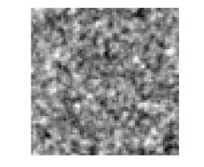
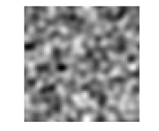
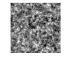
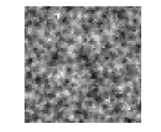
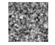
(a)                  (b)                  (c)                  (d)                   (e)

Figure 1: (a): Realization of the Gaussian process (51). (b): Realization of the microcanonical gradient descent computed with $\Phi_{d}(x)=\Phi^{\mu}_{d}(x)=\|x\star h\|_{2}^{2}$. (c): Realization computed with a vector $\Phi_{d}(x)$ of $\bf l^{2}$ wavelet norms. (d): $\Phi_{d}(x)$ is composed of $\bf l^{1}$ wavelet norms. (e): $\Phi_{d}(x)$ is a scattering transform.

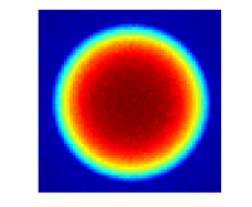
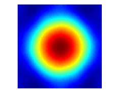
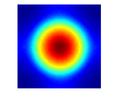
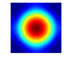
(a)                  (b)                  (c)                  (d)                   (e)

Figure 2: (a): Power spectrum of the original Gaussian process. (b): Estimation of the spectrum of a microcanonical gradient descent computed with the energy vector $\Phi_{d}(x)=\phi_{d}(x)=\|x\star h\|_{2}^{2}$. (c): The energy vector $\Phi_{d}(x)$ consists of $\bf l^{2}$ wavelet norms. (d): $\Phi_{d}(x)$ includes $\bf l^{1}$ wavelet norms. (e): $\Phi_{d}(x)$ includes $\bf l^{1}$ scattering norms.

Wavelet $\bf l^{2}$ norms

Let us now compute the gradient descent microcanonical measure $\mu_{n}$ with a wavelet $\bf l^{2}$ norm energy vector $\Phi_{d}$ in (42). We shall see that it can provide good approximations of Gaussian processes. The normalized variance $\sigma^{2}(\Phi_{d})$ in Table 1 remains small which indicates that this energy vector remains concentrated around its mean. Figure 1(c) shows a realization of the resulting microcanonical gradient descent model and Figure 2(c) gives an estimation of the power spectrum of this stationary process. This power spectrum is now much closer to the original power spectrum.

To understand this, observe that wavelet $\bf l^{2}$ norms specify the signal energy in the different frequency bands covered by each band-pass wavelet filter $\hat{\psi}_{j,q}({\omega})$:

$$\|x\star\psi_{j,q}\|^{2}=\sum_{\omega}|\hat{x}({\omega})|^{2}\,|\hat{\psi}_{j,q}({\omega})|^{2}.$$ (53)

The fact that the power spectrum remains nearly constant over the support of each $\hat{\psi}_{j,q}$ is a consequence of Theorem 3.4(iii). Indeed, suppose that $Lx$ is a linear operator which performs a permutation of the values of $\hat{x}({\omega}_{1})$ and $\hat{x}({\omega}_{2})$, for two non-zero frequencies ${\omega}_{1}$ and $\omega_{2}$ such that $\hat{\psi}_{j,q}({\omega}_{1})=\hat{\psi}_{j,q}({\omega}_{2})$ for all $j,q$. It is an orthogonal operator which preserves the mean (zero frequency) and it is a symmetry of $\Phi_{d}$. Theorem 3.4(iii) implies that the gradient descent measure $\mu_{n}$ is also invariant to the action of $L$ and is thus a stationary process whose power spectrum is the same at ${\omega}_{1}$ and ${\omega}_{2}$. This property is approximately valid for any frequencies ${\omega}_{1}$ and ${\omega}_{2}$ located near the center of the support of each $\hat{\psi}_{j,q}$, where it remains nearly constant and where all other $\hat{\psi}_{j^{\prime},q^{\prime}}$ nearly vanish. It implies that the spectrum of $\mu_{n}$ remains nearly constant in these frequency domain.

The energy concentration $e^{2}_{\mu_{n}}$ in Table 1 is small although not as small as $\sigma^{2}_{\mu}(\Phi^{\mu}_{d})$ which indicates the presence of a bias. To reduce this bias we must reduce the support size of each wavelet $\hat{\psi}_{j,q}$ where the spectrum must remain nearly constant. Appropriate wavelet design can yield arbitrarily small errors when $d$ increases.

Besides having an appropriate power spectrum, these microcanonical gradient descent models are also nearly Gaussian processes. This can be shown with a phase symmetry argument, which is explained without a formal proof. The wavelet norms in (53) and hence $\Phi_{d}(x)$ are invariant if we preserve $|\hat{x}({\omega})|$ but change the complex phase of $\hat{x}({\omega})$ for ${\omega}\neq 0$. Arbitrary rotations of the Fourier complex phases which transform real signals into real signals are linear orthogonal operators which preserve the stationary mean. As a result, Theorem 3.4 proves that the gradient descent process is invariant to any such Fourier phase rotation. This means that Fourier transforms of realizations of these microcanonical gradient descent processes have phases which are independent and uniformly distributed. Given a fixed power spectrum, a standard result based on the central limit theorem proves that stationary random processes with independent and uniformly distributed Fourier phases converge to a Gaussian processes when the dimension $d$ goes to $\infty$ [21]. Under appropriate hypotheses, microcanonical gradient descent processes conditioned by $\bf l^{2}$ wavelet norms will thus converge to Gaussian processes.

Wavelet $\bf l^{1}$ norms

Maximum entropy models conditioned by wavelet $\bf l^{1}$ norms capture sparsity with Laplacian distributions but do not approximate Gaussian processes accurately. Figure 1(d) shows samples of the microcanonical gradient processes computed with a wavelet $\bf l^{1}$ norm energy (44). The $\bf l^{1}$ norm constraints produce wavelet coefficients which are more sparse than a true Gaussian process. It creates images which are more piece-wise regular than in Figure 1(c). Errors are also visible in the resulting power spectrum shown in Figure 2(d). Table 1 shows that the resulting model error $e^{2}_{\mu_{n}}$ for the $\bf l^{1}$ norm wavelet vector is about $10$ times larger than with the $\bf l^{2}$ wavelet energy vector.

Scattering energy

The scattering energy vector (46) includes high order multiscale terms which can nearly reproduce the $\bf l^{2}$ norms of wavelet coefficients, as proved by Proposition 4.1. Table 1 gives the normalized variance $\sigma^{2}_{\mu}(\Phi_{d}(x))$ which shows that it concentrates nearly as well as wavelet $\bf l^{2}$ norm energy vectors, despite the fact that it is much larger. Figure 1(e) shows a realization of the scattering microcanonical gradient descent model and Figure 2(e) gives its power spectrum. It is nearly as precise as the $\bf l^{2}$ norm microcanonical model and the model error $e^{2}_{\mu_{n}}$ in Table 1 has about the same amplitude.

5.3 Ising Processes

We consider a two-dimensional Ising process with no outside magnetization, over a two-dimensional square lattice with periodic boundary conditions. We denote by $x(u)$ the spin values in $\{-1,1\}$. The Ising probability of a configuration $x$ is

$$p(x)={\cal Z}^{-1}\exp\left(-\beta\,\phi_{d}(x)\right)~{}~{}\mbox{with}~{}~{}\phi_{d}(x)=d^{-1}\sum_{u\in{\Lambda_{d}}}\sum_{u^{\prime}\in{\cal N}_{u}}x(u)x(u^{\prime}),$$ (54)

where ${\cal N}_{u}$ is the $4$ point neighborhood of $x(u)$ in the two-dimensional grid. The constant $\beta=(k_{B}T)^{-1}$ is the inverse temperature scaled by the Boltzmann constant $k_{B}$. In two dimension, the free energy can be exactly computed with the method of Onsager [36]. It has a phase transition when $T$ reaches a critical value $T_{c}\approx 2.27$. We study the approximation of Ising for several values of the temperature.

The complex behavior of Ising arises from the conjunction of the quadratic Hamiltonian with the binary constraint. This binary condition may be replaced by a condition on a fourth order moment to obtain the same critical behavior but we shall impose it here through first and second order moments. For all $x\in{\mathbb{R}}^{d}$, one has $\|x\|_{2}\leq\|x\|_{1}\leq\sqrt{d}\|x\|_{2}$, and $\|x\|_{1}=\sqrt{d}\,\|x\|_{2}$ if and only if $|x(u)|$ is constant. It follows that

$$\forall u~{},~{}x(u)=\pm 1\Leftrightarrow\|x\|_{1}=\|x\|_{2}^{2}=d~{}.$$

We can thus impose that $x$ is binary by adding $d^{-1}\|x\|_{2}^{2}$ and $d^{-1}\|x\|_{1}$ into the energy vector. The resulting microcanonical interaction energy for $x\in{\mathbb{R}}^{\Lambda_{d}}$ is

$$\Phi^{\mu}_{d}(x)=\{d^{-1}\|x\|_{2}^{2}\,,\,d^{-1}\|x\|_{1}\,,\,\phi_{d}(x)\}.$$ (55)

If we remove the ${\bf l}^{1}$ term, this energy is quadratic and the maximum entropy model is therefore a stationary Gaussian process.

The Ising model has a phase transition at the critical temperature $T_{c}\approx 2.27$, from an ‘ordered’ to a ‘disordered’ state. The spin spatial correlation exhibits a characteristic scale $\xi(T)$ for $T>T_{c}$ and ${\mathbb{E}}{\{X(u)X(u+r)\}}\simeq e^{-|r|/\xi(T)}$ [28], with $\xi(T_{c})=0$. The correlation is self-similar at $T=T_{c}$ and ${\mathbb{E}}{\{X(u)X(u+r)\}}\simeq|r|^{-1/2}$.

Figure 2(a) gives two realizations of Ising for a large temperature (bottom) and a temperature just above the critical temperature (top). Figure 2(b) shows realizations of the microcanonical gradient descent process computed with the Ising energy vector $\Phi^{\mu}_{d}$. The first column of Table 2 shows that $e^{2}_{\mu_{n}}(\Phi^{\mu}_{d})\gg\sigma^{2}(\mu(\Phi^{\mu}_{d})$ which means that the microcanonical gradient descent does not converge to a microcanonical set for $\epsilon$ small. Near the critical temperature, the gradient descent microcanonical model is unable to recover low-frequency long-range structures which appear in Ising. This is due to a well-known instability near criticality.

	$\Phi_{d}=\Phi^{\mu}_{d}$	$\Phi_{d}=$Wavelet $\bf l^{2}$	$\Phi^{d}=$ Wavelet $\bf l^{1}$	$\Phi_{d}=$ Scattering
${\rm dim}(\Phi_{d}(x))$	3	42	42	116
$\sigma_{\mu}^{2}(\Phi_{d})$ $T=2.2$	6e-6	3e-4	4e-4	6e-4
$e_{\mu_{n}}^{2}(\Phi_{d})$ $T=2.2$	2e-2	7e-2	5e-2	9e-3
$\sigma_{\mu}^{2}(\Phi_{d})$ $T=3$	3e-6	2e-5	4e-5	4e-5
$e_{\mu_{n}}^{2}(\Phi_{d})$ $T=3$	7e-3	4e-2	5e-2	5e-3

Table 2: The first line gives the dimension of each energy vectors $\Phi_{d}(x)$. We consider two Ising processes (54), computed near the critical temperature $T=2.2$ and at a larger temperature $T=3$. The table gives the normalized variance $\sigma_{\mu}^{2}(\Phi_{d})$ and the Ising energy concentration $e_{\mu_{n}}^{2}(\Phi_{d})$, for different $\Phi_{d}(x)$.

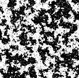
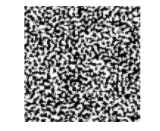
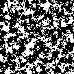
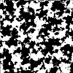
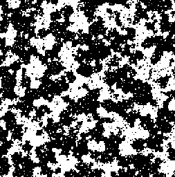
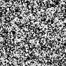
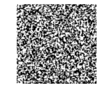
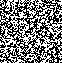
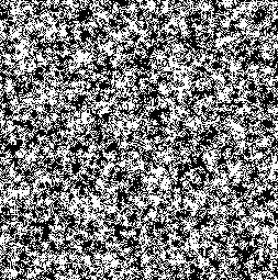
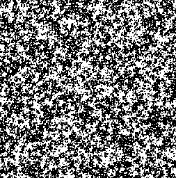
(a)                  (b)                  (c)                  (d)                   (e)

Figure 3: (a): Realizations of an Ising process near the critical temperature $T=2.2$ (top), and for $T=3$ (bottom). (b): Realizations computed with the microcanonical gradient descent with $\Phi_{d}=\Phi^{\mu}_{d}$. (c): $\Phi_{d}(x)$ includes $\bf l^{2}$ wavelet norms. (d): $\Phi_{d}(x)$ includes $\bf l^{1}$ wavelet norms. (e): $\Phi_{d}(x)$ includes $\bf l^{1}$ scattering norms.

Renormalization and wavelets

As in Wilson renormalization group, wavelets separate the frequency components of $x$ into dyadic frequency annulus. Relations between wavelets and renormalization group decompositions were studied by Battle [5]. In the following, we give a qualitative argument to explain how to approximate the Ising potential with wavelet norms.

Since $x(u)\in\{-1,1\}$, for an integer $p$

$$x(u)x(u^{\prime})=1-2^{-1}\,{|x(u)-x(u^{\prime})|^{p}}$$

so we can rewrite the Ising energy $\phi_{d}(x)=d^{-1}\sum_{u\in{\Lambda_{d}}}\sum_{u^{\prime}\in{\cal N}_{u}}x(u)x(u^{\prime})$ satisfies

$$d-\phi_{d}(x)=2^{-1}\sum_{u\in{\Lambda_{d}}}\sum_{u^{\prime}\in{\cal N}_{u}}|x(u)-x(u^{\prime})|^{p}=\|\Delta_{1}x\|_{p}^{p}+\|\Delta_{2}x\|_{p}^{p},$$ (56)

with $\Delta_{1}x(u_{1},u_{2})=x(u_{1},u_{2})-x(u_{1},u_{2}-1)$ and $\Delta_{2}x(u_{1},u_{2})=x(u_{1},u_{2})-x(u_{1}-1,u_{2})$.

The equivalence of $\bf l^{p}$ norms of increments and $\bf l^{p}$ norms of wavelet coefficients is established in [35]. For any $p>1$ there exists $A_{p}>0$ and $B_{p}>0$ so that for any $x\in{\bf l^{2}}({\mathbb{Z}}^{2})$

$$A_{p}\sum_{j,q}2^{-jp}\|x\star\psi_{j,q}\|_{p}^{p}\leq\|\Delta_{1}x\|_{p}^{p}+\|\Delta_{2}x\|_{p}^{p}\leq B_{p}\sum_{j,q}2^{-jp}\|x\star\psi_{j,q}\|_{p}^{p}.$$ (57)

For $p=1$ the upper-bound remains valid but to get a lower-bound we must replace the sum over $j,q$ by a sup operator. However, we conjecture that there exists $A_{1}$ which verifies the lower bound for $p=1$ when the values of $x(u)$ are restricted to $\{-1,1\}$. With equations (56) and (57) one can approximate the Ising energy $\phi_{d}(x)$ with discrete wavelet ${\bf l}^{p}$ norms computed at all scales $2^{j}\leq 2^{J}=d$. We limit the maximum scale $2^{J}$ independently of $d$, which is set to be the largest correlation length of the process.

As in Section 5.3, we capture the fact that $x(u)\in\{-1,1\}$ by including a condition on $d^{-1}\|x\|_{1}$ and $d^{-1}\|x\|_{2}^{2}$. The resulting energy vector for $p=1$ and $p=2$ is

$$\Phi_{d}(x)=\Big{\{}d^{-1}\|x\|_{2}^{2}\,,d^{-1}\|x\|_{1}\,,\,d^{-1}\,\|x\star\psi_{j,q}\|_{p}^{p}\Big{\}}_{j\leq J,q\leq Q}.$$ (58)

Table 2 shows the normalized variance $\sigma^{2}(\Phi_{d})$ is smaller at high temperature than near critical temperature but the separation of scale still provides a high concentration of $\Phi_{d}(x)$ for an Ising process, close to the critical temperature. Figure 3(c,d) show realizations of a microcanonical gradient descent Ising model computed with the wavelet energy (58) for $p=1$ and $p=2$. Near critical temperature, the microcanonical gradient descent still converges where as it was not the case when the energy was calculated directly with the Ising Hamiltonian energy $\phi_{d}(x)$ in Figure 3(b). The scale separation avoids having an ill-conditioned gradient descent. The Ising approximation with an $\bf l^{2}$ energy vector for $p=2$ amounts to compute a Gaussian approximation of Ising, which is not precise, when we are close to the critical temperature [28]. One can indeed visualize important differences with the statistical distribution of original Ising in Figure 3(a). Table 2 shows that the model error $e^{2}_{\mu_{n}}$ is smaller at higher temperature.

The Ising approximation with an $\bf l^{1}$ energy vector has about the same error as the model computed with an $\bf l^{2}$ energy vector. Near the critical temperature, the microcanonical models obtained with $\bf l^{1}$ wavelets norms shown in Figure 3(d) are more piecewise regular than the ones in Figure 3(c) obtained with wavelet $\bf l^{2}$ norms. This is due to the wavelet coefficient sparsity imposed by these $\bf l^{1}$ norms.

Scattering energy

A scattering energy vector is defined for Ising process, by complementing the scattering energy vector (46) with $\bf l^{1}$ and $\bf l^{2}$ norms of $x$ in order to impose that $x(u)$ takes binary values:

$$\Phi_{d}(x)=\Big{\{}d^{-1}\|x\|_{2}^{2}\,,\,d^{-1}\|x\|_{1}\,,\,d^{-1}\sum_{u\in{\Lambda_{d}}}x(u)\,,\,d^{-1}\,\|x\star\psi_{j,q}\|_{1}\,,\,d^{-1}\,\||x\star\psi_{j,q}|\star\psi_{j^{\prime},q^{\prime}}\|_{1}\Big{\}}_{j,j^{\prime}\leq J,q,q^{\prime}\leq Q}~{}.$$ (59)

Table 2 shows that the normalized variance of the scattering energy is about twice larger than for $\bf l^{2}$ wavelet energy vectors. Figure 3(e) shows realizations of microcanonical gradient descent models computed with this scattering energy vector. They are visually difficult to distinguish from realization of the original Ising process above the critical temperature and close to the critical temperature. Table 2 shows that the model error $e^{2}_{\mu_{n}}$ is about $10$ times smaller than with $\bf l^{2}$ or $\bf l^{1}$ wavelet energies.

These numerical experiment seem to indicate that scattering microcanonical gradient descents can provide accurate model of Ising even close to critical temperature. However, this needs to be sustained by a better mathematical of these approximations, by analyzing the preservation of symmetries.

5.4 Point Processes

Point processes provide powerful models of stochastic geometry, with applications in many areas of astrophysics, neuroscience, finance and computer vision. Realizations of point processes have a support reduced to isolated points. We first show that this sparsity can be captured by wavelet $\bf l^{1}$ norms. We then study approximations of point processes and shot noises with microcanonical models defined by scattering coefficients.

Support from wavelet $\bf l^{1}$ norms

We prove that wavelet $\bf l^{1}$ norms capture important geometric properties of the support of point processes. Young’s inequality implies that

$$\|x\star\psi_{j,q}\|_{1}\leq\|x\|_{1}\,\|\psi_{j,q}\|_{1}.$$

If $x$ is a Dirac in ${\Lambda_{d}}$ then this inequality is an equality. Conversely, the following theorem, proved in Appendix I proves that if this inequality is an equality then $x$ is a sum of Diracs, with conditions on their distances. The inner product and norm of $v$ and $v^{\prime}$ in ${\mathbb{R}}^{\ell}$ is written $v.v^{\prime}$ and $\|v\|$.

We suppose that wavelets are defined from a mother wavelet $\psi(u)$ which is continuous with $\psi(0)\neq 0$. We suppose that $\psi(u)=|\psi(u)|\,e^{i\,\varphi(\xi.u)}$ where $\xi\in{\mathbb{R}}^{\ell}$ and the complex phase $\varphi$ is a bi-Lipschitz function. We may choose linear phase $\varphi(\xi.u)=\xi.u$. This wavelet is rotated and dilated $\psi_{j,q}(u)=2^{-j\ell}\psi(2^{-j}r_{q}^{-1}u)$, where the $r_{q}$ are $Q\geq\ell$ different rotations in ${\mathbb{R}}^{\ell}$. The following theorem applies to these wavelets.

Theorem 5.1.

(i) If $\|x\star\psi_{j,q}\|_{1}=\|x\|_{1}\,\|\psi_{j,q}\|_{1}$ then $x$ is non-zero at $u$ and $u^{\prime}$ only if $\xi_{q}.(u-u^{\prime})=0$ with $\xi_{q}=r_{q}\xi$ or if $|\xi_{q}.(u-u^{\prime})|\geq C\,2^{j}~{}$, where $C>0$ does not depend on $x$.
(ii) Suppose that $\psi$ has a compact support, and that $x$ has a support which is a union of isolated points with distances larger than $\Delta$. If $x^{\prime}$ satisfies

$$\forall q\leq Q\,,\,\forall j\leq\log_{2}\Delta~{},~{}\|x^{\prime}\star\psi_{j,q}\|_{1}=\|x\star\psi_{j,q}\|_{1}~{}~{}\mbox{and}~{}~{}\|x^{\prime}\|_{1}=\|x\|_{1}~{}$$ (60)

then the support of $x^{\prime}$ is a set of isolated points of distances larger than $C\,\Delta$, where $C>0$ does not depend on $x$.

In dimension $\ell=2$, property (i) of Theorem 5.1 proves that the support of $x$ is included in straight lines perpendicular to $\xi_{q}$, whose distances are larger than $C\,2^{j}$. If this is valid for several $q$ then the support is included over intersections of non-parallel lines and hence reduced to isolated points, as proved by property (ii).

If $x$ is a realization of a point process, its support is a union of isolated points whose minimum distance depends the point process distribution. If we construct an $\epsilon=0$ microcanonical model with wavelet $\bf l^{1}$ norms then property (ii) proves that all realizations of this microcanonical model will also be a point process with a similar separation between points.

Microcanonical models of point processes

We study microcanonical models of point processes with wavelet $\bf l^{1}$ norms and scattering coefficients. A point process $N$ on ${\mathbb{R}}^{\ell}$ is a measure whose support is composed of isolated points. Second-order point processes [8] are those satisfying ${\mathbb{E}}[N(C)^{2}]<\infty$ for all bounded Borel sets $C\subset{\mathbb{R}}^{\ell}$. If $N$ is a stationary, second-order point process then one can define its associated Bartlett spectral measure [8] $P_{N}$, which generalizes the power spectrum of second-order stationary processes.

Given a non-negative stationary process $\lambda(t)$, $t\in{\mathbb{R}}^{\ell}$, a Cox process $N$ is defined as a Poisson process conditional on $\lambda$ with intensity $\lambda(t)$. Important geometric information of $N$ is captured by its Bartlett power spectrum, which satisfies $P_{N}(d{\omega})=P_{\lambda}(d{\omega})+{\mathbb{E}}(\lambda)\,\delta(d{\omega})$ [8]. Shot noises are classes of random processes defined by convolutions of point processes with a filter $h(t)$

$$X(t)=N\star h(t)~{}.$$

The filter $h(t)$ can be interpreted as a pattern which is randomly translated at point locations and added. It may also be the transfer function of a detector measuring the point-process. In this case, the power spectrum of $X$ is $P(d{\omega})=P_{N}(d{\omega})\,|\hat{h}({\omega})|^{2}$, which mixes the geometric information of $N$ with the profile of the filter $h$. We will show that they can be disentangled by a wavelet scattering transform.

The loss of information in the power spectrum is due to the fact that it does not measure scale interactions. When there is a scale separation between $N$ and $h$, ie

$${\mathbb{E}}({\lambda})^{2}\gg\int u^{2}|h(u)|^{2}du$$ (61)

then for sufficiently small scales $2^{j}$, one can verify [11] that

$$|X\star\psi_{j,q}|=|N\star(\psi_{j,q}\star h)|\approx N\star|\psi_{j,q}\star h|~{}$$ (62)

with high probability, due to the fact that the events in $N$ rarely interact at spatial scales $j$ such that $2^{j}\ll{\mathbb{E}}({\lambda})$. From this approximation, it follows that for sufficiently large scale gap $j^{\prime}\gg j$, we have

$$||X\star\psi_{j,q}|\star\psi_{j^{\prime},q^{\prime}}|\approx C_{j,q}|N\star\psi_{j^{\prime},q^{\prime}}|~{},$$ (63)

since $|\psi_{j,q}\star h|\star\psi_{j^{\prime},q^{\prime}}\approx C_{j,q}\delta\star\psi_{j^{\prime},q^{\prime}}$. Second order scattering coefficients, indexed with pairs $(j,q,j^{\prime},q^{\prime})$, thus provide measurements that convey spectral information about the point process $N$ as $(j^{\prime},q^{\prime})$ varies, disentangled from the spectral information of $h$.

We illustrate this phenomena by considering a two-dimensional Cox point process $N(u)$, whose rate $\lambda(u)$ is a stationary Gaussian process whose power spectrum is concentrated in the low-frequencies, and with an integral scale of $100$ pixels. This Cox process is convolved with a pattern $h(u)$ with zero mean and small spatial support of $5$ pixels. We build microcanonical models with energy vectors $\Phi_{d}(x)$ defined by wavelet $\bf l^{1}$ norms or scattering coefficients, computed up to a maximum scale $2^{J}$. For the shot noise measure $\mu$ shown in Figure 4(a), Table 3 gives the normalized variances $\sigma^{2}_{\mu}={{{\mathbb{E}}_{\mu}}(\|\Phi_{d}(x)-{\mathbb{E}}(\Phi_{d}(x))\|^{2})}/{\|{{\mathbb{E}}}_{\mu}(\Phi_{d}(x))\|^{2}}$ as a function of the maximum scale $2^{J}$. Although the size of scattering vectors for large $J$ becomes relatively large, the normalized variance remains small which proves that these energy vectors remain concentrated around their mean, for images of size $d=256^{2}$. We can thus define microcanonical models from an energy vector $\Phi_{d}(\bar{x})$ calculated from the realization $\bar{x}$ shown in Figure 4(a).

	$J=2$		$J=4$		$J=6$
	$\sigma_{\mu}^{2}(\Phi_{d})$	$\dim(\Phi_{d})$	$\sigma_{\mu}^{2}(\Phi_{d})$	$\dim(\Phi_{d})$	$\sigma_{\mu}^{2}(\Phi_{d})$	$\dim(\Phi_{d})$
$\Phi_{d}$: Wavelet $\bf l^{1}$	$410^{-6}$	$21$	$3\,10^{-6}$	$38$	$3\,10^{-6}$	$52$
$\Phi_{d}$: Scattering	$8\,10^{-6}$	$88$	$10^{-5}$	$422$	$10^{-5}$	$580$

Table 3: Estimated normalized variance for wavelet $\bf l^{1}$ norm and scattering energy vectors $\Phi_{d}$, at different maximum scales $2^{J}$. They are computed for a shot noise of size $d=256^{2}$ defined from a Cox point process. Figure 4(a) shows a realization.

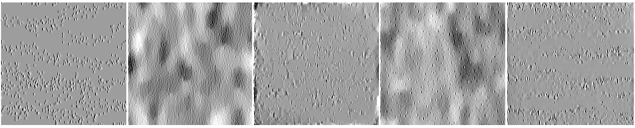
(a)                  (b)                  (c)                  (d)                   (e)

Figure 4: (a): Realization of a shot noise computed with a Cox process. (b,c): Realizations of a gradient descent process, computed with an energy $\Phi_{d}$ including wavelet $\bf l^{1}$ norms of maximum scale respectively $2^{J}=8$ and $2^{J}=64$. (d,e): Same computed with an energy $\Phi_{d}$ including scattering $\bf l^{1}$ norms of maximum scale respectively $2^{J}=8$ and $2^{J}=64$.

Figure 4 gives realizations of microcanonical gradient descent models computed from wavelet $\bf l^{1}$ norms and scattering energies, at different maximum scales $2^{J}$. Figure 4(b,d) are computed with $2^{J}=8$. These microcanonical models can only capture sparsity properties up to this maximum scale. At larger scale, the entropy maximisation creates Gaussian random process like variations having a uniform low-frequency spectrum. Figure 4(c,e) are microcanonical realizations computed at a larger maximum scale $2^{J}=64$. In this case, wavelet $\bf l^{1}$ norm and scattering microcanonical models capture the point process sparsity. The geometry of the shot noise is defined by the stationary rate $\lambda(u)$ which has relatively high frequency oscillations vertically but low frequency variations horizontally. The scattering model Figure 4(e) captures this distribution thanks to second order coefficients. This is not the case for the $\bf l^{1}$ norm model in Figure 4(c) which can not reproduce the low-frequency horizontal alignments.

5.5 Image and Audio Texture Synthesis

An image or an audio texture is usually modeled as the realization of a stationary process. Modeling textures amounts to compute an approximation of this stationary process given a single realization. A texture synthesis then consists in calculating new realizations from this stochastic model, which are hopefully perceptually identical to the original texture sample, although different if considered as deterministic signals. As opposed to the Gaussian, Ising or point process examples, since we do not know the original stochastic process, perceptual comparisons are the only criteria used to evaluate a texture synthesis algorithm. Microcanonical models can be considered as texture models computed from an energy function $\Phi_{d}(x)$ which concentrate close to its mean. We review previous work and give results obtained with a scattering microcanonical gradient descent model.

Geman and Geman [24] have introduced macrocanonical models based on Markov random fields. They provide good texture models as long as these textures are realizations of random processes having no long range correlations. Several approaches have then been introduced to incorporate long range correlations. Heeger and Bergen [26] capture texture statistics through the marginal distributions obtained by filtering images with oriented wavelets. This approach has been generalized by the macrocanonical Frame model of Mumford and Zhu [48], based on marginal distributions of filtered images. The filters are optimized by trying to minimize the maximum entropy conditioned by the marginal distributions. Although the Cramer-Wold theorem proves that enough marginal probability distributions characterize any random vector defined over ${\mathbb{R}}^{d}$ the number of such marginals is typically intractable, which limits this approach.

Portilla and Simoncelli [38] made important improvements to these texture models, with wavelet transforms. They capture the correlation of the modulus of wavelet coefficients with a covariance matrix which defines an energy vector $\Phi_{d}(x)$. Although they use a macrocanonical maximum entropy formalism, their algorithm computes a microcanonical estimation from a single realization, with alternate projections as opposed to a gradient descent. This approach was extended to audio textures by McDermott and Simoncelli [34]. A scattering representation is related to Portilla and Simoncelli model but covariance coefficients are replaced by a much smaller number of scattering ${\bf l}^{1}$ norms.

Excellent texture synthesis have recently been obtained with deep convolutional neural networks. In [23], the authors consider a deep VGG convolutional network, trained on a large-scale image classification task. The energy vector $\Phi_{d}(x)$ is defined as the spatial cross-correlation values of feature maps at every layer of the VGG networks. This energy vector is calculated on a particular texture image. Texture syntheses of very good perceptual quality are calculated with a gradient descent microcanonical algorithm initialized on random noise. However, the dimension of this energy vector $\Phi_{d}(x)$ is larger than the dimension $d$ of $x$. These estimators are therefore not statistically consistent and have no asymptotic limit.

In the following, we give results obtained with different wavelet microcanonical models computed on a collection of natural image and auditory textures. The Brodatz image texture dataset consists of 155 texture classes, with a single 512 $\times$ 512 sample per class. Auditory textures are taken from McDermott and Simoncelli [34], which contains 1 second samples of different sounds.

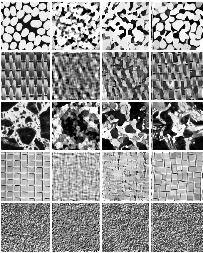
(a)                    (b)                   (c)                   (d)

Figure 5: (a): Original texture. (b): texture synthesized with a microcanonical gradient descent model with a vector $\Phi_{d}(x)$ of wavelet $\bf l^{2}$ norms. (c): $\Phi_{d}(x)$ has wavelet $\bf l^{1}$ norms. (d): $\Phi_{d}(x)$ has wavelet scattering coefficients.

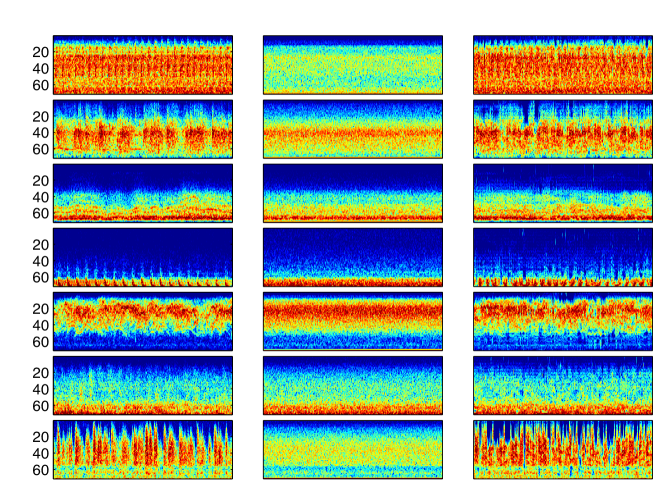
(a)                    (b)                   (c)

Figure 6: (a): Spectrograms of original audio textures produced (from to to bottom) by jackhammer, applause, wind, helicopter, sparrows, train, rusting paper. (b): Spectrograms of an audio texture synthesized with a microcanonical gradient descent model with a vector $\Phi_{d}(x)$ of wavelet $\bf l^{2}$ norms. (c): Spectrogram produced with a vector $\Phi_{d}(x)$ of wavelet scattering coefficients.

Since we have a single realization of each texture, we can not compute the concentration properties of energy vectors over these textures. Figure 5(a) gives input examples $\bar{x}$ corresponding to realizations of different stationary processes $X(u)$. Figure 5(b) shows texture samples obtained with a microcanonical gradient descent computed with an energy vector $\Phi_{d}(x)$ of wavelet $\bf l^{2}$ norm. It provides a good model for the bottom texture which is nearly Gaussian but it otherwise destroys the texture geometry. Figure 5(c) displays textures obtained with a vector $\Phi_{d}(x)$ of wavelet $\bf l^{1}$ norms. Their wavelet coefficients are more sparse than in Figure 5(b) which produces more “piecewise regular” images, but it does improve the texture geometry. On the contrary, scattering microcanonical textures in Figure 5(d) have a geometry which is much closer to original textures. Scattering coefficients can be interpreted as convolutional deep neural networks computed with predefined wavelet filters [10] as opposed to filters learned on a supervised image classification problem as in VGG.

The reconstruction of auditory textures is computed with a one-dimensional Gabor wavelet transform [9] with $Q=12$ scales per octave. Auditory textures have a rich mixture of homogeneous and impulsive, transient components, as well as amplitude and frequency modulation phenomena. Figure 6(a) displays the spectrograms of original auditory textures $\bar{x}$. Figure 5(b) shows the spectrogram of Gaussian texture models calculated with a microcanonical gradient descent computed with an energy vector $\Phi_{d}(x)$ of wavelet $\bf l^{2}$ norm. The global spectral energy is preserved but the time variations which destroys ability to recognize these audio textures. On the contrary, Figure 5(c) shows that audio textures synthesized with a scattering energy vector have spectrograms with the same type of time intermittency as the original textures. The resulting audio textures are perceptually difficult to distinguish from the original ones.

Synthesis from scattering energy vectors can also destroy some certain structures which affect their perceptual quality. This is the case for speech or music backgrounds which have harmonic alignments which are not reproduced by scattering coefficients. Deep convolutional network reproduce image and audio textures of better perceptual quality than scattering coefficients, but use over 100 times more parameters. Much smaller models providing similar perceptual quality can be constructed with wavelet phase harmonics for audio signals [33] or images [47], which capture alignment of phases across scales. However, understanding how to construct low-dimensional multiscale energy vectors to approximate random processes remains mostly an open problem.

6 Conclusion

This paper shows that gradient descent microcanonical models computed with multiscale energy vectors can provide powerful models to approximate large classes of stationary processes. Realizations of such models are calculated with a gradient descent algorithm which is much faster than MCMC algorithms, used to sample from macrocanonical models.

We introduced a mathematical framework to analyze the statistical and algorithmic properties of these microcanonical gradient descent models. Our analysis reveals that, whereas micrcocanonical gradient descent measures do not generally agree with the microcanonical maximum entropy measure, they have rich regularities through shared symmetries, and, under appropriate conditions, are shown to converge to the microcanonical ensemble. In the high-dimensional setting, gradient descent microcanonical models are therefore valid alternatives to classic macrocanonical and microcanonical maximum entropy measures, thanks to their computational tractability.

However, many mathematical questions remain open. For instance, on the convergence properties of this gradient descent algorithm, on the choice of the energy vector to obtain accurate approximations of random processes, and on the extension to locally stationary processes.

Acknowledgements: SM: This work was supported by the ERC grant InvariantClass 320959. JB: This work was partially supported by the Alfred P. Sloan Foundation, by NSF RI-1816753, and by Samsung DMC. We thank Zhengdao Chen and Ofer Zeitouni for valuable comments and fixes to the current manuscript, and the anonymous referees for their high-quality, valuable feedback.

Appendix A Proof of Theorem 3.1

A.1 Proof of part (i)

The main technical challenge to prove (26) is to show that assumption (C) is sufficient to guarantee that $|J\Phi_{d}x|^{-1}$ is integrable. Since $\Phi_{d}$ is Lipschitz from assumption (A), the coarea formula proves that for any integrable function $g(x)$

$$\int_{{{B}}}g(x)\,|J\Phi_{d}x|\,dx=\int_{{\mathbb{R}}^{K}}\,\int_{\Phi_{d}^{-1}(y)}g(x)\,d{\cal H}^{{d}-K}(x)\,dy~{}.$$ (64)

In order to apply (64) to $|J\Phi_{d}(x)|^{-1}$ and obtain the expression of $H(\mu^{\mathrm{mi}}_{d,\epsilon})$, we need to show that $|J\Phi_{d}(x)|^{-1}$ is integrable in $\Phi^{-1}_{{d},\epsilon}(y)$. Using the notation for each Jacobian column (22), we verify that $|J\Phi_{d}(x)|$ satisfies

$$|J\Phi_{d}(x)|\geq d^{-{\ell}}\max\left\{|\text{det}[{J}U(\bar{X}_{1}),\dots,{J}U(\bar{X}_{K})]|,\dots,|\text{det}[{J}U(\bar{X}_{\tilde{{d}}+1}),\dots,{J}U(\bar{X}_{\tilde{{d}}+K})]|\right\}~{},$$ (65)

where $\bar{X}_{i}$ is a projection of $x$ onto disjoint subsets of $2\Delta+1$ coordinates, and $\tilde{{d}}\geq{d}(2\Delta+1)^{-1}=\Theta({d})$.

We will show that for ${d}$ large enough and arbitrary $R>0$,

$$\int_{|x|_{\infty}<R}|J\Phi_{d}(x)|^{-1}dx<\infty~{},$$ (66)

by interpreting (66) as proportional to the expected value of ${\mathbb{E}}_{X\sim\mathrm{Unif}({d},R)}|J\Phi_{d}(X)|^{-1}$. Since $\Phi^{-1}_{d,\epsilon}(y)$ is a compact set thanks to assumption (B), it is bounded, so $\Phi^{-1}_{{d},\epsilon}(y)\subseteq\{x\,;\,|x|_{\infty}<R\}$ for some $R$, which proves that $|J\Phi_{d}(x)|^{-1}$ is integrable in $\Phi^{-1}_{{d},\epsilon}(y)$.

For that purpose, let us prove that assumption (C) from (25) is sufficient to guarantee (66). If $F_{V}(y)$ denotes the cumulative distribution function of a random variable $V$, and $Y$ denotes the r.v. $Y=|\text{det}[{J}U(\bar{X}_{1}),\dots,{J}U(\bar{X}_{K})]|$, we first observe that thanks to (65) it is sufficient to show that

$$F_{Y}(y)\lesssim y^{\eta}~{},~{}\text{for some }\eta>0~{},~{}(y\to 0)~{}.$$ (67)

Indeed, since $V=|J\Phi_{d}(X)|\geq\max(Y_{1},\dots,Y_{\tilde{{d}}})$ with $Y_{i}$ independent and identically distributed, we have that

$$F_{V}(y)\leq F_{Y}(y)^{\tilde{{d}}}\simeq y^{\eta\tilde{{d}}}~{}.$$

It follows that

$${\mathbb{E}}_{X\sim\mathrm{Unif}({d},R)}|J\Phi_{d}(X)|^{-1}\leq\int v^{-1}f_{V}(v)dv=C+\int_{0}^{R^{\prime}}v^{-2}F_{V}(v)dv<\infty$$

as soon as $\tilde{{d}}\eta>1$, which will happen for large enough ${d}$.

Let us thus prove (67) by induction on $K$. When $K=1$, $V=|\text{det}{J}U(\bar{X}_{1})|=|{J}U(\bar{X}_{1})|$ and assumption (C) directly implies that

$$F_{V}(y)=P(V\leq y)\lesssim y^{\eta}~{}.$$

Now, suppose (67) is true for $K-1$ and let us prove it for $K$. We use the following lemma:

Lemma A.1.

We say that a bounded random vector $Z$ in $B(K,R)\subset{\mathbb{R}}^{K}$ has property (*) if there exists $\eta>0$ such that

$$~{}\forall~{}\mathcal{S}\subset{\mathbb{R}}^{K}\text{ Lebesgue measurable}~{},~{}P(Z\in\mathcal{S})\lesssim|\mathcal{S}|^{\eta}~{}.$$

If $Z$ has property (*) and $K>1$, then $Z_{H}$, the orthogonal projection of $Z$ onto any hyperplane, also has property (*), and

$${\mathbb{E}}(\|Z\|^{-\eta})<C_{R,\eta}~{}.$$ (68)

Before proving the lemma, let us conclude with (67). By denoting $Z_{i}={J}U(\bar{X}_{i})$, $i=1\dots K$, and assuming $\|Z_{1}\|>0$, one Gram-Schmidt iteration yields

$$|\text{det}\left[Z_{1},\dots,Z_{K}\right]|=\|Z_{1}\||\text{det}\left[\tilde{Z}_{2},\dots,\tilde{Z}_{K}\right]|~{},$$

where $\tilde{Z}_{i}$ is the projection of $Z_{i}$ onto the orthogonal complement of $Z_{1}$. Using assumption (C), we use lemma A.1 to observe that $\tilde{Z}_{i}$, $i=2,\dots K$ also satisfies assumption (C), since we compute it with an orthogonal projection that depends only on $Z_{1}$, which is independent from all the $Z_{i}$, $i\geq 2$. Thus by induction hypothesis and using (68) we obtain

$$F_{Y}(y)=P\left(|\text{det}\left[Z_{1},\dots,Z_{K}\right]|\leq y\right) = P\left(\|Z_{1}\||\text{det}\left[\tilde{Z}_{2},\dots,\tilde{Z}_{K}\right]|\leq y\right)$$

$$= {\mathbb{E}}_{Z_{1}}P\left(|\text{det}[\tilde{Z}_{2},\dots,\tilde{Z}_{K}]|\leq y\|Z_{1}\|^{-1}~{}|~{}Z_{1}\right)$$

$$\leq {\mathbb{E}}_{Z_{1}}y^{\eta}\|Z_{1}\|^{-\eta}\lesssim y^{\eta}~{},$$

which proves (67).

Let us finally prove lemma A.1. Let $\mathcal{S}_{H}$ be a measurable set in a given hyperplane $H$ of dimension $K-1$, and let $\tilde{\mathcal{S}}=\mathcal{S}_{H}\times(-R,R)$ be the corresponding cylinder in $B(K,R)$. By definition, we have

$$P(Z_{H}\in\mathcal{S}_{H})=P(Z\in\tilde{\mathcal{S}})\leq|\tilde{\mathcal{S}}|^{\eta}=|\mathcal{S}_{H}|^{\eta}(2R)^{\eta}$$

which proves that $Z_{H}$ also has the property (*).

Finally, let us show that ${\mathbb{E}}(\|Z\|^{-\eta})<C_{R,\eta}$. For positive random variables we have

$${\mathbb{E}}(\|Z\|^{-\eta}) = \int_{0}^{R}r^{-\eta}f_{\|Z\|}(r)dr$$

$$= R^{\eta}-\lim_{r\to 0}r^{-\eta}P(\|Z\|\leq r)+\eta\int_{0}^{R}r^{-\eta-1}P(\|Z\|\leq r)dr$$

$$\leq R^{\eta}+C\eta\int_{0}^{R}r^{-\eta-1+\eta K}dr\leq C_{R,\eta}~{},$$

since $K>1$ and $\eta>0$. This proves lemma A.1 and thus (26). $\square$

To prove that ${\gamma_{d}}(y)$ is integrable on any bounded set, we apply the coarea formula to (64) to $g(x)=|J_{K}\Phi x|^{-1}\,1_{\mathcal{A}}(\Phi x)$ where $\mathcal{A}$ is bounded:

$$\int_{{{\mathbb{R}}^{d}}}1_{\mathcal{A}}(\Phi x)\,dx=\int_{\mathcal{A}}\,\int_{\Phi^{-1}(z)}|J_{K}\Phi x|^{-1}\,d{\cal H}^{{d}-K}\,dz=\int_{\mathcal{A}}{\gamma_{d}}(z)\,dz~{}.$$

If $\mathcal{A}$ is a compact set then by assumption (B) it follows immediately that

$$\int_{{{\mathbb{R}}^{d}}}1_{\mathcal{A}}(\Phi x)\,dx=\int_{\Phi^{-1}(\mathcal{A})}dx\leq|B_{2,d}(C\sqrt{(}d))|<\infty,$$ (69)

which proves that ${\gamma_{d}}$ is integrable on a compact.

A.2 Proof of part (ii)

Let us now prove that for each ${d}$, $\gamma_{d}(y)$ can only vanish when $\mathrm{dist}(y,\overline{\Phi_{d}({{\mathbb{R}}^{d}})})\leq c/d$ for some fixed constant $c$. We will exploit the relationship between the sets $\Phi_{d}({\mathbb{R}}^{d})$ and $\Phi_{{d}/2}({\mathbb{R}}^{d/2})$ thanks to the fact that $\Phi_{d}$ is an average potential over the domain.

The inequality (27) proves that ${\gamma_{d}}(y)=0$ only if $\int_{\Phi^{-1}(y)}d{\cal H}^{{d}-K}=0$. Since in finite integer dimensions the Hausdorff measure ${\cal H}^{{\ell}}$ is a multiple of the Lebesgue measure in ${\mathbb{R}}^{{\ell}}$, it is sufficient to show that whenever $y\in(\Phi_{d}({{\mathbb{R}}^{d}}))^{\circ}$ , the set $\Phi^{-1}(y)$ has positive Lebesgue measure of dimension ${d}-K$.

Without loss of generality, assume that $\Phi=(\phi_{1},\dots,\phi_{K})$ are linearly independent functions. Otherwise, if there were a linear dependency of the form

$$\sum_{k\leq K}\alpha_{k}\phi_{k}(x)\equiv 0~{},$$

then $\Phi_{d}({{\mathbb{R}}^{d}})=\partial\Phi_{d}({{\mathbb{R}}^{d}})$, thus $\Phi_{d}({{\mathbb{R}}^{d}})^{o}$ is empty and there is nothing to prove.

Let us write ${d}=r^{\ell}$, with $r$ denoting the length of the cube ${\Lambda_{d}}$. Suppose first that $r$ is even. Given $y\in(\Phi_{2^{-{\ell}}{d}}({\mathbb{R}}^{2^{-{\ell}}{d}}))^{\circ}$ we will see that there exists $x\in\Phi^{-1}(y)$ whose Jacobian $J\Phi(x)$ has rank $K$. Then, by the Implicit Function Theorem, one can find a local reparametrization of $\Phi^{-1}(y)$ in a small neighborhood $V$ of the form $x=(v,\varphi(v))$ such that

$$\{(v,\varphi(v));v\in V\subset{\mathbb{R}}^{{d}-K},\varphi:V\to{\mathbb{R}}^{K}\}=\{(v,v^{\prime})\in V\times\varphi(V);\,\Phi(v,v^{\prime})=y\}~{},$$

which has positive Lebesgue measure of dimension ${d}-K$.

Suppose first that $\Delta=1$. Then the sets $\mathcal{S}_{d}=\Phi_{d}({{\mathbb{R}}^{d}})\subset{\mathbb{R}}^{K}$ satisfy $\mathcal{S}_{{d}}\subseteq\mathcal{S}_{q^{\ell}{d}}$ for $q=1,2,\dots$. Indeed, given $y\in\mathcal{S}_{d}$, by definition there exists $x\in{{\mathbb{R}}^{d}}$ with $\Phi_{d}(x)=y$. Consider $\tilde{x}=(x,\dots,x)^{\otimes{\ell}}\in{\mathbb{R}}^{q^{\ell}{d}}$, a tiling of $x$, $q$ times along each dimension. By construction, $\tilde{x}$ satisfies $\Phi_{q^{\ell}{d}}(\tilde{x})=y$ and therefore $y\in\mathcal{S}_{q^{\ell}{d}}$.

Now, consider $y\in\mathcal{S}_{d}^{\circ}\subseteq\mathcal{S}_{2^{\ell}{d}}^{\circ}$. If $\Phi_{d}$ was a smooth $C^{s}$ map, with $s>d-K$, then by Sard’s theorem, the image of critical points $\{x\in{{\mathbb{R}}^{d}};|J\Phi_{d}(x)|<K\}$ has zero Lebesgue measure in $\mathcal{S}_{d}$. Although one can extend Sard’s theorem to weaker regularity assumptions [3], for our purposes we will use a weaker and simpler property that does not require the smoothness assumption, as described in the following lemma:

Lemma A.2.

Under the assumptions of the theorem, the set $\mathcal{A}=\{y\in{\mathbb{R}}^{K};~{}0<{\gamma_{d}}(y)<\infty\}$ is dense in $\Phi_{d}({{\mathbb{R}}^{d}})$, and for each $y\in\mathcal{A}$ there exists $x\in\Phi^{-1}_{d}(y)$ with $|J\Phi_{d}(x)|>0$.

It follows that for a sufficiently small $\delta>0$, a neighborhood $B(y,\delta)\subset\mathcal{S}_{d}$ of $y$ necessarily contains two points $y_{1}=y+\eta$, $y_{2}=y-\eta$ such that $\Phi_{d}^{-1}(y_{1})$ or $\Phi_{d}^{-1}(y_{2})$ contain a regular point. Let $x_{1}\in\Phi_{d}^{-1}(y_{1})$ and $x_{2}\in\Phi_{d}^{-1}(y_{2})$ be two points such that at least one is regular. The point $\tilde{x}=(x_{1}^{\otimes{\ell}},x_{2}^{\otimes{\ell}})\in{\mathbb{R}}^{2^{\ell}{d}}$, obtained by concatenating $x_{1}$ and $x_{2}$ along the first coordinate, and tiling them along the rest, satisfies

$$\Phi_{2^{\ell}{d}}(\tilde{x})=\frac{1}{2}\left(\Phi_{{d}}(x_{1})+\Phi_{d}(x_{2})\right)=y~{},\text{ and}$$

$$|J\Phi_{2^{\ell}{d}}(\tilde{x})|\geq\max(|J\Phi_{{d}}(x_{1})|,|J\Phi_{{d}}(x_{2}|)>0~{},$$

which shows that we have just found an element $\tilde{x}$ of $\Phi_{2^{\ell}{d}}^{-1}(y)$ with $\text{rank}(J\Phi_{2^{\ell}{d}}(\tilde{x}))=K$.

Suppose finally that $\Delta>1$. The proof follows the same strategy, but we need to handle the border effect introduced by the support $\Delta$. In that case, given $y\in\mathcal{S}_{d}$, we consider $\tilde{x}=(x,u,x)^{\otimes{\ell}}$, where $u$ has $2(\Delta-1)$ zero coordinates and $x\in\Phi_{d}^{-1}(y)$. That is, we consider $2^{{\ell}}$ copies of $x$ separated by $2(\Delta-1)$ zeroes along each dimension so that their potential functions do not interact.

Let $\tilde{{d}}=(2r+2(\Delta-1))^{\ell}$. It follows that

$$\Phi_{\tilde{{d}}}(\tilde{x})=\frac{2^{\ell}{d}\Phi_{d}(x)}{\tilde{{d}}}=\left(1+\frac{\Delta-1}{r}\right)^{-{\ell}}\Phi_{d}(x)=\left(1+\frac{\Delta-1}{{d}^{1/{\ell}}}\right)^{-{\ell}}y~{},$$

which shows that $\text{dist}(y;\mathcal{S}_{\tilde{{d}}})\lesssim C{\ell}\|y\|/{{d}^{1/{\ell}}}$ for any $y\in\mathcal{S}_{d}$.

Now consider $y$ in the open set $C_{d}=\mathcal{S}_{d}\cap\mathcal{S}_{\tilde{{d}}}$, such that $\text{dist}(y,\partial\mathcal{S}_{d})\geq\|y\|{\ell}\Delta{d}^{-1/{\ell}}$. It follows from the previous argument that there exists small $\delta>0$ and $x_{1}\in\Phi_{d}^{-1}(y_{1})$ with $|J\Phi_{d}(x_{1})|>0$ and $y_{1}\in B(y,\delta)\cap\mathcal{S}_{d}\cap\mathcal{S}_{\tilde{{d}}}$. We verify from the assumption that

$$y_{2}=2\left(1+\frac{\Delta-1}{r}\right)^{{\ell}}y-y_{1}\in\mathcal{S}_{d}~{},$$

and therefore for any $x_{2}\in\Phi_{d}^{-1}(y_{2})$ the point $\tilde{x}=(x_{1};u,x_{2})^{\otimes{\ell}}$ that contains $2^{{\ell}-1}$ copies of $x_{1}$ and $2^{{\ell}-1}$ copies of $x_{2}$ satisfies by construction

$$\Phi(\tilde{x})=\frac{{d}2^{{\ell}-1}y_{1}+{d}2^{{\ell}-1}y_{2}}{\tilde{{d}}}=y~{}\text{ and }$$

$\text{rank}(J\Phi_{2{d}}(\tilde{x}))=K$. Finally, the case where $r$ is odd is treated analogously, but splitting the coordinates into $\lfloor\frac{r}{2}\rfloor$ and $\lceil\frac{r}{2}\rceil$ parts.

It remains to prove Lemma A.2. We know from part (i) that thanks to the coarea formula,

$$\forall~{}\epsilon~{}\forall y\in(\Phi_{d}({{\mathbb{R}}^{d}}))^{\circ},~{}0<\int_{\|z-y\|\leq\epsilon}\gamma_{d}(z)dz=\int_{\|\Phi(x)-y\|\leq\epsilon}dx<\infty~{}.$$

It follows that $\mathcal{A}=\{z;~{}0<\gamma_{d}(z)<\infty\}$ is dense in $\Phi_{d}({{\mathbb{R}}^{d}})$. But if $y\in\mathcal{A}$, by definition this implies that $\Phi_{d}^{-1}(y)$ has positive $({d}-K)$-Hausdorff measure, and that there is necessarily $x\in\Phi_{d}^{-1}(y)$ with $|J\Phi_{d}(x)|^{-1}<\infty$, therefore with a full-rank Jacobian. $\square$

A.3 Proof of part (iii)

In order to prove (28), we will again exploit the relationships between the sets $\mathcal{S}_{d}=\Phi_{d}({{\mathbb{R}}^{d}})$ as ${d}$ grows. We also first establish the result for $\Delta=1$, and then generalize it to $\Delta>1$. Denote $F_{{d},\epsilon}={d}^{-1}H(\mu^{\mathrm{mi}}_{d,\epsilon})$ the entropy rate associated with $y$ and $\epsilon$ and $\Omega_{{d},\epsilon}(y)=\{x;\|\Phi_{d}(x)-y\|\leq\epsilon\}$.

In the last section we proved that when $\Delta=1$, $\mathcal{S}_{d}\subseteq S_{q^{\ell}{d}}$ for $q=1,2,\dots$. For any $\epsilon>0$ and $y\in\mathcal{S}_{d}$, observe that

$$\Omega_{{d},\epsilon}(y)\underbrace{\otimes\dots\otimes}_{\text{$2^{{\ell}}$ times}}\Omega_{{d},\epsilon}(y)\subseteq\Omega_{2^{\ell}{d},\epsilon}(y)~{}.$$ (70)

Indeed, if $x\in\Omega_{{d},\epsilon}(y)\underbrace{\otimes\dots\otimes}_{\text{$2^{{\ell}}$ times}}\Omega_{{d},\epsilon}(y)$, then by definition $x=(x_{1},\dots,x_{2^{{\ell}}})$ with

$$\|\Phi_{d}(x_{i})-y\|\leq\epsilon~{}.$$

But

$$\Phi_{2^{\ell}{d}}(x)=2^{-{\ell}}\sum_{i=1}^{2^{{\ell}}}\Phi_{d}(x_{i})$$

and $\|\Phi_{2^{\ell}{d}}(x)-y\|\leq\epsilon$ by the convexity of the ${\bf l}^{2}$ norm, thus $x\in\Omega_{2^{\ell}{d},\epsilon}(y)$. It follows that

$$F_{2^{\ell}{d},\epsilon}={d}^{-1}2^{-{\ell}}H(\mu^{\mathrm{mi}}_{2^{\ell}{d},\epsilon})\geq{d}^{-1}2^{-{\ell}}\log\left(\left[\int_{\|\Phi_{d}(x)-y\|\leq\epsilon}dx\right]^{2^{{\ell}}}\right)=F_{{d},\epsilon}~{}.$$ (71)

Thus, for any fixed ${d}_{0}$, $y\in\mathcal{S}_{{d}_{0}}$ and $\epsilon>0$, the sequence $F_{k}=F_{2^{k{\ell}}{d}_{0},\epsilon}$ is increasing. Also, thanks to assumption (B), we have that

$$\forall~{}{d}~{},~{}x\in\Omega_{{d},\epsilon}(y)\implies\|x\|\leq C\sqrt{d}(\|y\|+\epsilon)~{},$$

which implies that $|\Omega_{{d},\epsilon}(y)|\leq|B_{d}(\sqrt{d}R_{0})|$. Therefore

$$\forall~{}{d}~{},F_{{d},\epsilon}^{y}\leq{d}^{-1}\log|B_{d}(\sqrt{d}R_{0})|~{},$$

and we verify from $|B_{d}(R)|=\frac{\pi^{d/2}}{\Gamma(d/2+1)}R^{d}$ that $|B_{d}(\sqrt{d}R_{0})|\simeq\tilde{K}^{d}$ with $\tilde{K}=2\pi R_{0}^{2}e$, which shows that $\lim_{d\to\infty}d^{-1}\log|B_{d}(\sqrt{d}R_{0})|=\log\tilde{K}$ and thus that the entropy rate $F_{k}$ is also upper bounded, and therefore its limit exists $\lim_{k\to\infty}F_{k}=\bar{F}~{}.$ We shall see later that the limit does not depend upon the choice of ${d}_{0}$.

Let us now prove the case when $\Delta>1$. The idea is to show that (70) is now valid up to an error that becomes small as ${d}$ increases, provided that the potential $U$ is Holder continuous.

Consider $y\in\mathcal{S}_{d}$. Given $\epsilon>0$, we form

$$\Psi_{2^{\ell}{d},\epsilon}(y)=\left(\Omega_{{d},\epsilon}(y)\right)^{\otimes 2^{{\ell}}}$$

as the Cartesian product of $2^{{\ell}}$ copies of $\Omega_{{d},\epsilon}(y)$. When $\Delta=1$, we just saw that

$$\Psi_{2^{\ell}{d},\epsilon}(y)\subseteq\Omega_{2{d},\tilde{\epsilon}}(y)$$ (72)

with $\epsilon=\tilde{\epsilon}$, but when $\Delta>1$, let us see how to increase $\tilde{\epsilon}$ so that (72) is verified. Given $x\in\Psi_{2^{\ell}{d},\epsilon}(y)$, we write $x=(x_{1},\dots,x_{2^{{\ell}}})$ to denote its projections into each of the $2^{{\ell}}$ subdomains $C_{1,{d}},\dots,C_{2^{{\ell}},{d}}$ of size ${d}$. We have

$$\Phi_{2^{\ell}{d}}(x) = \frac{\sum_{n}Ux(n)}{2^{{\ell}}{d}}$$ (73)

$$= 2^{-{\ell}}\sum_{k=1}^{2^{{\ell}}}{d}^{-1}\left(\sum_{n\in C_{k,{d}}^{\circ}}Ux(n)+\sum_{n\in\partial C_{k,{d}}}Ux(n)\right)~{},$$

where each $C_{k,{d}}^{\circ}$ contains the interior of the domain that does not interact with the other domains, and $\partial C_{k,{d}}=C_{k,{d}}\setminus C_{k,{d}}^{\circ}$. We have $|\partial C_{k,{d}}|={d}-({d}^{1/{\ell}}-2\Delta)^{{\ell}}$, thus

$${d}^{-1}|\partial C_{k,{d}}|=1-(1-2\Delta{d}^{-1/{\ell}})^{{\ell}}\lesssim\frac{\ell\Delta}{{d}^{1/{\ell}}}~{}.$$ (74)

Since $|Ux(n)|\leq B\|x\|^{\alpha}$ with $\alpha<2/{\ell}$ by the Holder assumption, and $\|x\|\leq C\sqrt{d}$ by assumption (B), we have $|Ux(n)|\leq B^{\prime}d^{\alpha/2}$. It follows from (73) and (74) that

$$\|\Phi_{2^{\ell}{d}}(x)-y\| = \left\|2^{-\ell}\sum_{k=1}^{2^{{\ell}}}\left[{d}^{-1}\left(\sum_{n\in C_{k,{d}}^{\circ}}Ux(n)+\sum_{n\in\partial C_{k,{d}}}Ux(n)\right)-y\right]\right\|$$

$$\leq 2^{-{\ell}}\sum_{k=1}^{2^{{\ell}}}\left(\|\Phi_{d}(x_{i})-y\|+2B^{\prime}d^{\alpha/2}(1-(1-2\Delta{d}^{-1/{\ell}})^{{\ell}})\right)$$

$$\leq \epsilon+o\left({d}^{\frac{\alpha}{2}-\frac{1}{{\ell}}}{\ell}\Delta\right)~{},$$

Thus by taking $\tilde{\epsilon}=\epsilon+o\left({d}^{\frac{\alpha}{2}-\frac{1}{{\ell}}}{\ell}\Delta\right)$ (72) is verified. By denoting $\nu=\frac{\alpha}{2}-\frac{1}{{\ell}}$, it follows that the entropy rate $F_{{d},\epsilon}$ satisfies

$$F_{{d},\epsilon}\leq F_{2^{\ell}{d},\epsilon+\tilde{\ell}{d}^{\nu}}~{},$$

with $\tilde{\ell}=C\Delta{\ell}$, and $\nu<0$ since $\alpha<2/{\ell}$. By repeating the inequality for sufficiently large ${d}$ and $k=1,2,\dots$ and $\epsilon>0$ we have

$$F_{{d},\epsilon}\leq F_{{d}2^{k{\ell}}\,,~{}\epsilon+\tilde{{\ell}}{d}^{\nu}\sum_{k^{\prime}=0}^{k}2^{k^{\prime}{\ell}\nu}}\leq F_{{d}2^{k{\ell}},2\epsilon}\leq\tilde{C}~{},$$ (75)

and thus by defining

$$F_{\infty,\epsilon}:=\lim_{k\to\infty}F_{{d}_{0}2^{k{\ell}},\epsilon_{k}}~{},\text{ with }\epsilon_{k}=\epsilon+\tilde{{\ell}}{d}_{0}^{\nu}\sum_{k^{\prime}=0}^{k}2^{{\ell}\nu k^{\prime}}$$ (76)

we have shown that its entropy rate is well-defined for each $\epsilon>0$ and ${d}_{0}$ sufficiently large.

It remains to be shown that this limit does not depend upon ${d}_{0}$. Suppose $F_{\infty,\epsilon,0}\neq F_{\infty,\epsilon,1}$ where $F_{0}$ is associated with ${d}_{0}$ and $F_{1}$ is associated with ${d}_{1}$, and suppose ${d}_{1}>{d}_{0}$ without loss of generality. Let $r_{i}={d}_{i}^{1/{\ell}}$ for $i=0,1$.

Observe that an analogous argument to (73) shows that if $r=r_{a}+r_{b}$, then

$$F_{r^{\ell},\tilde{\epsilon}}\geq\frac{r_{a}}{r}F_{r_{a}^{\ell},\epsilon}+\frac{r_{b}}{r}F_{r_{b}^{\ell},\epsilon}~{},$$ (77)

and

$$F_{l^{\ell}{d},\tilde{\epsilon}}\geq F_{{d},\epsilon}~{}\text{for }l=1,2,\dots~{},$$ (78)

with $\tilde{\epsilon}=\epsilon+o\left({d}^{\nu}{\ell}\Delta\right)$. Consider now large integers $k$ and $\tilde{k}\simeq\sqrt{k}$, and let $q,\tilde{q}$ denote respectively the quotient and residual such that

$$r_{1}2^{k}=r_{0}2^{\tilde{k}}q+\tilde{q}$$

with $0\leq\tilde{q}<r_{0}2^{\tilde{k}}$. Then, for any $\delta>0$, by choosing $k$ large enough we obtain from (77) and (78) that

$$|F_{{d}_{1}2^{k{\ell}},\tilde{\epsilon}}-F_{1}| \leq \delta/4~{},$$

$$|F_{{d}_{0}2^{{\ell}\tilde{k}}q^{\ell},\tilde{\epsilon}}-F_{0}| \leq \delta/4~{},\text{ and }$$

$$|F_{{d}_{1}2^{k{\ell}},\bar{\epsilon}}-F_{{d}_{0}2^{\tilde{k}{\ell}}q^{\ell},\tilde{\epsilon}}| \leq \delta/4~{},$$ (79)

with $\bar{\epsilon}=\tilde{\epsilon}+o\left({d}^{\nu}{\ell}\Delta\right)$.

Finally, let us show that $F_{{d},\epsilon}$ is continuous with respect to $\epsilon$ for $\epsilon>0$. Let us denote $\gamma_{{d},\epsilon}=\int_{\|z-y\|\leq\epsilon}{\gamma_{d}}(z)dz$. Since $F_{{d},\epsilon}={d}^{-1}\log(\gamma_{{d},\epsilon}^{y})$ and $\gamma_{d}(y)>0$ for all $y\in\mathcal{S}_{d}^{\circ}$ from the previous section, it is sufficient to show that $\gamma_{{d},\epsilon}$ is continuous with respect to $\epsilon$. Let $\tilde{\epsilon}=\epsilon+\delta$ with $\epsilon>0$, and suppose $\delta>0$ without loss of generality. By denoting $Q(\delta,\epsilon,y)=\{z\,;\,\epsilon<\|z-y\|\leq\epsilon+\delta\}$, we have

$$|\gamma_{{d},\tilde{\epsilon}}-\gamma_{{d},\epsilon}| = \int_{\epsilon<\|z-y\|\leq\epsilon+\delta}{\gamma_{d}}(z)dz=\int{\gamma_{d}}(z){\bf 1}_{Q(\delta,\epsilon,y)}(z)dz$$

$$:= \int{\gamma_{d}}_{\delta}(z)dz$$

For each $z$, ${\gamma_{d}}_{\delta}(z)={\gamma_{d}}(z){\bf 1}_{Q(\delta,\epsilon,y)}(z)$ converges pointwise to $0$ as $\delta\to 0$, except for a set of measure zero, $\{z;\|z-y\|=\epsilon\}$. Also, $|{\gamma_{d}}_{\delta}|\leq{\gamma_{d}}$, which is integrable in $\Phi({{\Omega_{d}}})$ by part (i). We can thus apply the dominated convergence theorem, and conclude that

$$\lim_{\delta\to 0}\int{\gamma_{d}}_{\delta}(z)dz=\int\left(\lim_{\delta\to 0}{\gamma_{d}}_{\delta}(z)\right)dz=0~{},$$

which shows that $\gamma_{{d},\epsilon}$ is continuous with respect to $\epsilon$.

It follows from (A.3) that

$$|F_{{d}_{1}2^{k{\ell}},\tilde{\epsilon}}-F_{{d}_{0}2^{\tilde{k}{\ell}}q^{\ell},\tilde{\epsilon}}|\to 0~{}\text{as }k\to\infty~{},$$

but $F_{{d}_{1}2^{k{\ell}},\tilde{\epsilon}}\to F_{1}$ and $F_{{d}_{0}2^{\tilde{k}{\ell}}q^{\ell},\tilde{\epsilon}}\to F_{0}$ as $k\to\infty$, which is a contradiction with the fact that $F_{0}\neq F_{1}$. $\square$

Appendix B Proof of Corollary 3.2

We saw in Theorem 3.7 that the entropy rate of the microcanonical measure can be measured with the co-area formula as ${d}^{-1}H(\mu^{\mathrm{mi}}_{d,\epsilon})={d}^{-1}\log\int_{\|z-y\|\leq\epsilon}{\gamma_{d}}(z)dz~{}$ and that ${\gamma_{d}}(z)>0$ in the interior of $\Phi_{d}({{\mathbb{R}}^{d}})$. As $\epsilon\to 0$, we can interpret the previous formula in terms of an $L^{1}({\mathbb{R}}^{K})$ approximate identity $h_{\epsilon}(z)=C_{K}\epsilon^{-K}{\bf 1}_{\|z\|\leq\epsilon}(z)$:

$$C_{K}\epsilon^{-K}\int_{\|z-y\|\leq\epsilon}{\gamma_{d}}(z)dz={\gamma_{d}}\star h_{\epsilon}(y)\to{\gamma_{d}}(y)~{}~{}\text{as }\epsilon\to 0~{}$$

in $L^{1}({\mathbb{R}}^{K})$. One can verify that, by possibly reparametrising $\epsilon$, this implies pointwise convergence for almost every $y$, so

$$\left|\log\left(C_{K}\epsilon^{-K}\gamma_{d,\epsilon}^{y}\right)-\log\gamma_{d}(y)\right|\underset{\epsilon\to 0}{\to}0~{},~{}a.e.~{},$$ (80)

which shows that $d^{-1}H(p_{d,\epsilon}^{y})\simeq\frac{-K}{d}\log\epsilon$ as $\epsilon\to 0$ $\square$.

Appendix C Proof of Proposition 3.3

Properties (A) and (B) are verified for (i-ii) because the potentials $U$ are continuous and the resulting features $\Phi$ always include ${d}^{-1}\|x\|^{2}$ respectively. We thus focus on proving property (C).

Part (i) is easily obtained, since the ${\bf l}^{2}$ wavelet model has a Jacobian $J\Phi(x)$ that is linear with respect to $x$, and therefore it has absolutely continuous density relative to the Lebesgue measure.

Part (ii) is proved by directly controlling $|J\Phi_{d}(x)|^{-1}$. A direct computation shows that $|J\Phi_{d}(x)|={d}^{-1}\sqrt{{d}\|x\|^{2}-\|x\|_{1}^{2}}$, which only vanishes when $|x|$ is a constant vector. Therefore, for $y\neq(\alpha,{\Lambda_{d}}\alpha)$, $\Phi^{-1}_{{d},\epsilon}(y)$ does not contain those points for sufficiently small $\epsilon$.

Let us now show part (iii). The Jacobian matrix in that case is given by

$$J\Phi_{d}(x)_{j}={d}^{-1}\text{Re}\left\{\left(\frac{x\star h_{j}}{|x\star h_{j}|}\right)\star h_{j}^{*}\right\}~{},$$

with $j\leq K$. We proceed by induction over the scale $K$. Suppose first $K=1$. Since $h_{j}$ has compact spatial support, its Fourier transform only contains a discrete number of zeros. Denote by $\Delta_{j}$ the spatial support of $h_{j}$. We can thus generate all but a zero-measure set of unitary signals $z$ with $z_{s}=e^{i\theta_{s}}$, $s=1\dots\Delta_{j}$ from the uniform measure over $x$ using $z=\frac{x\star h_{j}}{|x\star h_{j}|}$. In the uniform phase space defined by $\theta_{1},\dots,\theta_{\Delta_{j}}$, the event $|\text{det}\bar{J}U(\bar{X}_{1})|\leq y$ has a probability proportional to $y$, since it is equivalent to

$$\left|\sum_{s}\cos(\theta_{s})\mathrm{Re}(h_{j}^{*}(s))-\sum_{s}\sin(\theta_{s})\mathrm{Im}(h_{j}^{*}(s)\right|\leq y~{}.$$

Suppose now the result holds for the $K-1$ filters in the family with smallest spatial support, and let us show how to extend it to an extra filter $h_{K}$ with strictly larger spatial support. Among the variables $\bar{X}\in{\mathbb{R}}^{2\Delta+1}$, a subset of them, say $R_{K}$, only affect the $K$-th output corresponding to filter $h_{K}$. It follows that a set $S\subset{\mathbb{R}}^{K}$ with shrinking measure necessarily introduces constraints on the variables in $R_{K}$, and therefore $P(Z\in S)\leq|S|^{1/K}$ $~{}\square~{}.$

Appendix D Proof of Theorem 3.4

(i) Let us first prove that volume preserving symmetries of $\Phi_{d}(x)$ are symmetries of the microcanonical maximum entropy measure. If for all $x\in{\mathbb{R}}^{d}$, $\Phi_{d}(L^{-1}x)=\Phi_{d}(x)$ then a microcanonical set $\Omega_{d,\epsilon}$ is invariant to the action of $L$ and $L^{-1}$. Since $L$ preserves volume and hence the Lebesgue measure of a set, for any measurable set $\mathcal{A}$, since $\mu^{\rm mi}_{d,\epsilon}$ is supported over $\Omega_{d,\epsilon}$ and uniform relatively to the Lebesgue measure, we have

$$\mu^{\rm mi}_{d,\epsilon}[L^{-1}\mathcal{A}]=\mu^{\rm mi}_{d,\epsilon}[L^{-1}\mathcal{A}\cap\Omega_{d,\epsilon}]=\mu^{\rm mi}_{d,\epsilon}[L^{-1}(\mathcal{A}\cap\Omega_{d,\epsilon})]=\mu^{\rm mi}_{d,\epsilon}[\mathcal{A}\cap\Omega_{d,\epsilon}]=\mu^{\rm mi}_{d,\epsilon}[\mathcal{A}],$$

so $L$ is a symmetry of $\mu^{\rm mi}_{d,\epsilon}$.

(ii) We prove that symmetries of $\Phi_{d}(x)$ and $\mu_{0}$ are symmetries of $\mu_{n}$, by induction on $n$. It is trivially valid for $n=0$. Suppose now by induction that $\mu_{n}$ is invariant to the action of $L$ which is a symmetry of $\Phi_{d}$. From (31), $\mu_{n+1}=\varphi_{n,\#}\mu_{n}$, with

$$\varphi_{n}(x)=x-\kappa_{n}J\Phi_{d}(x)^{\top}(\Phi_{d}(x)-y)~{}.$$

Let us verify that $\varphi_{n}$ is equivariant to the action of $L$: $\varphi_{n}L^{-1}x=L^{-1}\varphi_{n}x$ for all $x$. Since $\Phi_{d}(L^{-1}x)=\Phi_{d}(x)$, and since $L$ is linear

$$J\Phi_{d}(L^{-1}x)^{\top}=L^{-1}(J\Phi_{d}(L^{-1}x))^{\top}=L^{-1}(J\Phi_{d}(x))^{\top}$$ (81)

so

$$\varphi_{n}L^{-1}x = L^{-1}x-\kappa_{n}J\Phi_{d}(L^{-1}x)^{\top}(\Phi_{d}(L^{-1}x)-y)$$

$$= L^{-1}x-L^{-1}\kappa_{n}J\Phi_{d}(x)^{\top}(\Phi_{d}(x)-y)$$

$$= L^{-1}\varphi_{n}x~{},$$

which proves that $\varphi_{n}$ is equivariant to the action of $L$. Moreover, if $\varphi_{n}$ is equivariant to the action of $L$ then we verify that it is equivariant to the action of $L^{-1}$. Also, observe that

$$\varphi_{n}^{-1}(L^{-1}(\mathcal{A})) = \{x;\varphi_{n}(x)\in L^{-1}\mathcal{A}\}$$

$$= \{x;L\varphi_{n}(x)\in\mathcal{A}\}$$

$$= \{x;\varphi_{n}(Lx)\in\mathcal{A}\}$$

$$= L^{-1}\varphi_{n}^{-1}(\mathcal{A})~{}.$$

Finally, using the definition of pushforward measure, $\mu_{n+1}=\varphi_{n,\#}\mu_{n}$, for any measurable $\mathcal{A}$, the induction hypothesis yields

$$\mu_{n+1}[L^{-1}\mathcal{A}] = \mu_{n}[\varphi_{n}^{-1}(L^{-1}\mathcal{A})]$$

$$= \mu_{n}[L^{-1}\varphi_{n}^{-1}(\mathcal{A})]=\mu_{n}[\varphi_{n}^{-1}(\mathcal{A})]$$

$$= \mu_{n+1}[\mathcal{A}]~{},$$

which proves that $\mu_{n+1}$ is also invariant to the action of $L$.

(iii) We prove that an orthogonal operator which preserves a stationary mean is a symmetry of a Gaussian measure $\mu_{0}$ of $d$ i.i.d Gaussian random variables. Applying the statement (ii) then implies the statement (iii). Let $m_{0}$ be the mean of each of the $d$ Gaussian random variables. The Gaussian measure $\mu_{0}$ is uniform over all spheres of ${\mathbb{R}}^{d}$ centered over the stationary mean $m_{0}\,{\bf 1}$. An orthogonal operator $L$ which preserves the stationary mean leaves invariant all spheres centered in $m_{0}\,{\bf 1}\in{\mathbb{R}}^{d}$. Indeed $L(m_{0}\,{\bf 1})=m_{0}\,{\bf 1}$ and $\|Lx\|^{2}=\|x\|^{2}$ so

$$\|Lx-m_{0}{\bf 1}\|^{2}=\|L(x-m_{0}{\bf 1})\|^{2}=\|x-m_{0}{\bf 1}\|^{2}.$$

If $S(m{\bf 1},r)$ is a sphere centered in $m{\bf 1}$ of radius $r$ then ${\mathbb{R}}^{d}=\cup_{(m,r)\in{\mathbb{R}}\times{\mathbb{R}}^{+}}S(m{\bf 1},r)$. So for any measurable set $\mathcal{A}$

$$\mu_{0}[L^{-1}\mathcal{A}] = \mu_{0}[L^{-1}\mathcal{A}\cap\cup_{(m,r)\in{\mathbb{R}}\times{\mathbb{R}}^{+}}S(m{\bf 1},r)]=\mu_{0}[\cup_{(m,r)\in{\mathbb{R}}\times{\mathbb{R}}^{+}}L^{-1}(\mathcal{A}\cap S(m{\bf 1},r))]$$

$$= \mu_{0}[\cup_{(m,r)\in{\mathbb{R}}\times{\mathbb{R}}^{+}}\mathcal{A}\cap S(m{\bf 1},r)]=\mu_{0}[\mathcal{A}],$$

so $L$ is a symmetry of $\mu_{0}$.

Appendix E Proof of Theorem 3.7

E.1 Proof of part (i)

Let us first show how the strict saddle condition (33) implies that the minimisation $\mathcal{E}(x)$ has no poor local minima. The statement follows directly from [30], which shows that when the saddle points are strict, gradient descent does not converge to those saddle points, up to a set of initialization values with Lebesgue measure $0$. Observe first that $\kappa_{n}<\eta^{-1}$ ensures that $\varphi_{n}(x)=x-\eta\nabla E(x)$ is a diffeomorphism for each $n$. Observe also that a critical point $x$ such that $\nabla{{E}}(x)=J\Phi_{d}(x)^{T}(\Phi_{d}(x)-y)=0$ necessarily falls into two categories. Either $\Phi_{d}(x)=y$, which implies that $x$ is a global optimum, or $x$ is such that $J\Phi_{d}(x)^{T}v=0$ with $v=\Phi_{d}(x)-y\neq 0$. We verify that assumption (33) implies that in that case $x$ is a strict saddle point by observing that the Hessian of ${{E}}$ satisfies

$$\nabla^{2}{{E}}(x)=\sum_{k=1}^{K}\nabla^{2}\Phi_{k}(x)v_{k}+J\Phi(x)^{T}J\Phi(x)~{}.$$

Since $\mu_{0}$ is absolutely continuous with respect to the Lebesgue measure, we can apply Theorem 2.1 from [37], and establish that gradient descent does not converge to any saddle point with probability 1.

Let us now prove that the hypothesis that $|J\Phi_{d}(x)|>0$ for $x\in\Phi_{d}^{-1}(y)$ with $y\in\Phi_{d}({{\mathbb{R}}^{d}})^{\circ}$, together with the strict saddle condition, implies that the gradient descent sequence $x_{n}$ has a limit $\lim_{n\to\infty}x_{n}$ (that may depend upon $x_{0}$). For that, we will apply the following result from [1]:

Theorem E.1.

If ${{E}}(x)$ is twice differentiable, has compact sub-level sets, and the Hessian $\nabla^{2}{{E}}(x)$ is non-degenerate on the normal space to the level set of local minimisers, then $x_{n}$ has a limit, denoted $x_{\infty}:=\lim_{n\to\infty}x_{n}$.

Indeed, since $\Phi_{d}$ satisfies assumption (B), it follows that the sub-level sets of ${{E}}$, $\{x;{{E}}(x)\leq t\}$ are compact for each $t$. We need to show that the Hessian of ${{E}}$ is non-degenerate on the normal space of $\Phi_{d}^{-1}(y)$. Since ${\gamma_{d}}>0$ for $y\in\Phi_{d}({{\mathbb{R}}^{d}})^{\circ}$ for sufficiently large ${d}$ from Theorem 3.1, $\Phi_{d}^{-1}(y)$ has positive ${d}-K$-dimensional Hausdorff measure, hence it is sufficient to show that $\nabla^{2}{{E}}(x)$ has $K$ strictly positive eigenvalues when $x\in\Phi^{-1}(y)$. But by definition,

$$\nabla^{2}{{E}}(x)=\sum_{k\leq K}\nabla^{2}\phi_{k}(x)(\phi_{k}(x)-y_{k})+J\Phi_{d}(x)^{T}J\Phi_{d}(x)~{},$$

thus

$$\nabla^{2}{{E}}(x)=J\Phi_{d}(x)^{T}J\Phi_{d}(x)~{}~{}\text{for }~{}x\in\Phi_{d}^{-1}(y)~{}.$$ (82)

Therefore, if $|J\Phi_{d}(x)|>0$ for $x\in\Phi_{d}^{-1}(y)$, we can apply Theorem E.1, and conclude that the iterates $x_{n}$ from gradient descent have a limit, for each $x_{0}\sim\mu_{0}$.

We have just proved that

$$\mathrm{P}_{\mu_{0}}\left\{(x_{n})_{n}\text{ is Cauchy}\right\}=1~{},$$

or, equivalently, that $X_{n}\sim\mu_{n}$ is almost surely Cauchy, which implies [41] that $\mu_{n}$ converges almost surely to a certain measure $\mu_{\infty}$. Moreover, since $\lim_{n\to\infty}\|\nabla{{E}}(x_{n})\|=0$, the strict saddle condition implies that $x_{n}$ does not converge to saddle points, so we conclude that necessarily

$$\mu_{\infty}\left[\Phi_{d}^{-1}(y)\right]=\mathrm{P}_{\mu_{0}}\left\{\lim_{n\to\infty}x_{n}\in\Phi_{d}^{-1}(y)\right\}=1~{},$$

therefore that $\mu_{\infty}$ is supported in the microcanonical ensemble $\Phi_{d}^{-1}(y)$, which finishes the proof. $\square$

E.2 Proof of part (ii)

We first compute how the entropy is modified at each gradient step. By definition of the pushforward measure, for any diffeomorphism $\varphi$ and any measurable $g$

$${\mathbb{E}}_{x\sim\varphi_{\#}\mu}g(x)={\mathbb{E}}_{x\sim\mu}g(\varphi(x))~{}.$$

Also, from a change of variables we have, by denoting $\tilde{\mu}=\varphi_{\#}\mu$, $\tilde{\mu}(x)=|J\varphi^{-1}(x)|\mu(\varphi^{-1}(x))~{},$ and thus

$$\log\tilde{\mu}(x)=\log\mu(\varphi^{-1}(x))-\log|J\varphi(\varphi^{-1}(x))|~{}.$$

It follows that

$$-{\mathbb{E}}_{x\sim\tilde{\mu}}\log\tilde{\mu}(x)=-{\mathbb{E}}_{x\sim\mu}\log{\mu}(x)+{\mathbb{E}}_{x\sim\mu}\log|J\varphi(x)|$$

and hence

$$H(\varphi_{\#}\mu)=H(\mu)-{\mathbb{E}}_{\mu}\log|J\varphi(x)|~{}.$$ (83)

The change in entropy by applying the diffeomorphism is thus given by the term ${\mathbb{E}}_{\mu}\log|J\varphi(x)|$, and thus the entropy of $\mu_{n}$ is given by

$$H(\mu_{n})=H(\mu_{0})-\sum_{n^{\prime}\leq n}{\mathbb{E}}_{\mu_{n^{\prime}}}\log|J\varphi_{n}(x)|$$

By definition, the Jacobian of $\varphi_{n}$ is

$$J\varphi_{n}(x)={\bf 1}-\gamma_{n}\left(\sum_{k\leq K}\nabla^{2}\phi_{k}(x)(\phi_{k}(x)-y_{k})+J\Phi_{d}(x)^{T}J\Phi_{d}(x)\right)~{}.$$ (84)

We know that $\Phi$ is Lipschitz, which implies that $\|J\Phi(x)\|\leq\beta$, and that $\nabla\Phi$ is also Lipschitz, meaning that $\|\nabla^{2}\phi_{k}(x)\|\leq\eta$ for all $k$. Applying the Cauchy-Schwartz inequality, it follows that

$$\left\|\sum_{k\leq K}\nabla^{2}\phi_{k}(x)(\phi_{k}(x)-y_{k})\right\|\leq\eta K\sqrt{{{E}}(x)}~{}.$$

We abuse notation and redefine $\eta:=\eta K$ since $K$ is a constant. Also, the term $J\Phi(x)^{T}J\Phi(x)$ is of rank at most $K$. We can thus write $J\varphi_{n}(x)$ as

$$J\varphi_{n}(x)=A_{n}(x)+B_{n}(x)~{},$$ (85)

with $A_{n}(x)$ full rank ${d}$ and with singular values within the interval $(1-\gamma_{n}\eta\sqrt{{{E}}(x)},1+\gamma_{n}\eta\sqrt{{{E}}(x)})$; and $-B_{n}(x)$ positive semidefinite of rank $K$, with singular values bounded by $\gamma_{n}\beta^{2}$. It follows that the singular values of $J\varphi_{n}(x)$, called $\lambda_{1},\dots,\lambda_{d}$, satisfy

$$|\log|J\varphi_{n}(x)|| \leq \sum_{i=1}^{d}|\log\lambda_{i}|$$

$$\leq \sum_{i=1}^{{d}-K}\max(|\log(1+\gamma_{n}\eta\sqrt{{{E}}(x)})|,|\log(1-\gamma_{n}\eta\sqrt{{{E}}(x)})|)$$

$$+\sum_{i=1}^{K}|\log(1-\gamma_{n}\beta^{2})|$$

$$\leq ({d}-K)\log(1+\gamma_{n}\eta\sqrt{{{E}}(x)})+K\log(1+\gamma_{n}\beta^{2})+o(\gamma_{n}^{2})$$

and thus up to second order terms we have

$${\mathbb{E}}_{\mu_{n}}\log|J\varphi_{n}(x)| \leq ({d}-K)\log\left(1+\gamma_{n}\eta{\mathbb{E}}_{\mu_{n}}\sqrt{{{E}}(x)}\right)+K\log\left(1+\gamma_{n}\beta^{2}\right)~{},$$ (86)

$$\leq ({d}-K)\gamma_{n}\eta{\mathbb{E}}_{\mu_{n}}\sqrt{{{E}}(x)}+K\gamma_{n}\beta^{2}~{},$$

where we have used Jensen’s inequality on the concave function $\log(1+x)$ and $\log(1+x)\leq x$ for $x\geq 0$ to obtain the inequality ${\mathbb{E}}\log(1+X)\leq\log(1+{\mathbb{E}}X)$. Denoting by $r_{n}={\mathbb{E}}_{\mu_{n}}\sqrt{{{E}}(x)}$ the average distance to the microcanonical ensemble at iteration $n$, it results from (86) that after $n$ steps of gradient descent the entropy rate has decreased at most

$$\left(1-\frac{K}{{d}}\right)\eta\sum_{n^{\prime}\leq n}\gamma_{n^{\prime}}r_{n^{\prime}}+\frac{K}{{d}}\beta^{2}\sum_{n^{\prime}\leq n}\gamma_{n^{\prime}}~{}.$$

Appendix F Proof of Corollary 3.8

The proof is a direct application of Theorem 3.7 and Sard’s theorem, that states that if $\Phi_{d}$ is a ${\bf C}^{\infty}$ Lipschitz function, then the image of its critical points $\{x~{},;\,|J\Phi_{d}(x)|=0\}$ has zero measure. We can thus apply Theorem E.1 from part (ii) of the proof of Theorem 3.7 for almost every $y$ $\square$.

Appendix G Proof of Theorem 3.9

We show that $\Phi_{d}(x)=\{{d}^{-1}\|x\star h_{k}\|_{2}^{2}\}_{k}$ satisfies the strict saddle condition. Here $x\in{\mathbb{R}}^{d}$, and we recall that the Fourier transform is defined as $\hat{x}(\omega)=\sum_{u}x(u)e^{-i\omega u2\pi/d}$, with $\omega\in(-d/2,d/2]$. The gradient of the loss function ${{E}}(x)=\frac{1}{2}\|\Phi(x)-y\|^{2}$ is

$$\nabla{{E}}(x)=J\Phi_{d}(x)^{T}(\Phi_{d}(x)-y)~{},$$

and its Hessian is

$$\nabla^{2}{{E}}(x)=\sum_{k}\nabla^{2}\phi_{k}(x)v_{k}+J\Phi_{d}(x)^{\top}J\Phi_{d}(x)~{},$$

where $v_{k}=\phi_{k}(x)-y_{k}$. Expressing the gradient and the Hessian in the Fourier domain yields

$$\nabla{{E}}(\hat{x}) = \hat{x}\cdot(\sum_{k}v_{k}|\hat{h_{k}}|^{2})$$ (87)

$$\nabla^{2}{{E}}(\hat{x})({\omega},{\omega}^{\prime}) = \sum_{k}v_{k}|\hat{h_{k}}({\omega})|^{2}\delta({\omega}-{\omega}^{\prime})+\hat{x}({\omega})|\hat{h_{k}}({\omega})|^{2}\hat{x}({\omega}^{\prime})^{*}|\hat{h_{k}}({\omega}^{\prime})|^{2}~{}.$$ (88)

The Hessian thus contains a diagonal term and a rank-$K$ term. We need to show that a critical point $x$ satisfying $\nabla{{E}}(\hat{x})=0$ with $\|v\|>0$ has a Hessian matrix with at least one negative eigenvalue. From (87), it follows that a critical point satisfies

$$\forall{\omega}~{},~{}\hat{x}({\omega})\cdot(\sum_{k}v_{k}|\hat{h_{k}}({\omega})|^{2})=0~{}.$$ (89)

Let $C=\{{\omega}~{};~{}\hat{x}({\omega})\neq 0\}$. The Hessian is expressed in terms of block matrices regrouping the frequencies in $C$ as

$$\nabla^{2}{{E}}(\hat{x})=\left(\begin{array}[]{c|c}\mathrm{M}&0\\ \hline\cr 0&\nabla^{2}_{C,C}\end{array}\right)~{},$$

where $\mathrm{M}$ is the diagonal matrix of size $(d-|C|)\times(d-|C|)$ given by the frequencies outside $C$, such that $\hat{x}({\omega})=0$:

$$\mathrm{M}_{\omega,\omega}=\sum_{k}v_{k}|\hat{h_{k}}({\omega})|^{2}~{},~{}\omega\notin C~{}.$$

We examine the diagonal block corresponding to $\mathrm{M}$. The image of $\Phi_{d}$ is the convex cone $\mathcal{C}$ in $\mathbb{R}_{+}^{K}$ determined by the directions $o_{\omega}=(|\hat{h_{1}}({\omega})|^{2},\dots,|\hat{h_{K}}({\omega}_{j})|^{2})\in{\mathbb{R}}^{K}$, ${\omega}=1\dots d$. Without loss of generality, we assume here that $\|o_{\omega}\|>0$ for all ${\omega}$, since frequencies that are invisible to all the filters do not play any role in the gradient descent. The target $y$ is by hypothesis in the interior of $\mathcal{C}$. Further, any two directions $o,o^{\prime}$ in $\mathcal{C}$ satisfy

$$\langle o,o^{\prime}\rangle = \sum_{k}|\hat{h_{k}}({\omega})|^{2}|\hat{h_{k}}({\omega}^{\prime})|^{2}>0~{},$$

since the filters have compact spatial support.

If $C$ is empty, then $x=0$, which implies that $v=\Phi(x)-y=-y$ has all its entries negative, and therefore $\text{diag}(\sum_{k}v_{k}|\hat{h_{k}}({\omega})|^{2})<0$. We shall thus assume in the following that $C$ is non-empty. Similarly, we verify that the space spanned by $o_{\omega}$, $\omega\in C$, cannot have full rank $K$. Indeed, if this was the case, the first order optimality condition (89) reveals that $v$ should be orthogonal to all directions $o_{\omega}$, $\omega\in C$. Since this system has rank $K$, this contradicts the fact that $v\neq 0$.

We can thus write $\mathcal{C}$ as generated by directions $\mathcal{O}_{C}=\{o_{\omega};\omega\in C\}$ and $\mathcal{O}_{\overline{C}}=\{o_{\omega};\omega\notin C\}$, with $|\mathcal{O}_{\overline{C}}|>0$, $|\mathcal{O}_{C}|>0$. Since $y$ is in the interior, it follows that

$$y=\sum_{\omega\in C}\beta_{\omega}o_{\omega}+\sum_{\omega\notin C}\gamma_{\omega}o_{\omega}~{},~{}\beta_{\omega},\gamma_{\omega}>0\forall~{}\omega~{}.$$ (90)

We need to show that there exists at least one $\omega\notin C$ such that $\langle v,o_{\omega}\rangle<0$. Suppose otherwise, i.e. that for all $\omega\notin C$, $\langle\Phi_{d}(x),o_{\omega}\rangle\geq\langle y,o_{\omega}\rangle$. Since $o_{\omega}\in\mathcal{O}_{C}\Rightarrow\langle\Phi_{d}(x),o_{\omega}\rangle=\langle y,o_{\omega}\rangle$ by the first order critical conditions, we have

$$\langle y,y\rangle = \sum_{\omega\in C}\beta_{\omega}\langle o_{\omega},y\rangle+\sum_{\omega\notin C}\gamma_{\omega}\langle o_{\omega},y\rangle$$ (91)

$$\leq \sum_{\omega\in C}\beta_{\omega}\langle o_{\omega},\Phi_{d}(x)\rangle+\sum_{\omega\notin C}\gamma_{\omega}\langle o_{\omega},\Phi_{d}(x)\rangle~{}.$$

On the other hand, from (90) we also have

$$\langle y,\Phi_{d}(x)\rangle=\sum_{\omega\in C}\beta_{\omega}\langle o_{\omega},\Phi_{d}(x)\rangle+\sum_{\omega\notin C}\gamma_{\omega}\langle o_{\omega},\Phi_{d}(x)\rangle~{},$$ (92)

and since $\Phi(x)=\sum_{\omega\in C}\alpha_{\omega}o_{\omega}$ is a linear combination of vectors in $\mathcal{O}_{\overline{C}}$, we also have $\langle\Phi(x),y\rangle=\langle\Phi(x),\Phi(x)\rangle$. This implies from (91) that

$$\langle y,y\rangle\leq\langle y,\Phi_{d}(x)\rangle=\langle\Phi_{d}(x),\Phi_{d}(x)\rangle~{},$$ (93)

which leads to $y=\Phi(x)$ and therefore $v=0$, which is a contradiction.

Finally, if $x\in\Phi_{d}^{-1}(y)$ for $y\in\Phi_{d}({{\mathbb{R}}^{d}})^{\circ}$, then $y$ falls necessarily inside the convex hull of $\mathcal{C}$, which implies that $\{\nabla\phi_{k}(x)=\hat{x}({\omega})\cdot|\hat{h}_{k}|^{2}({\omega})\}_{k\leq K}$ have rank $K$. This concludes the proof $\square$.

Appendix H Proof of Proposition 4.1

If $\gamma=0$ then (39) proves that

$$\|x\|_{2}^{2}=\|x\star\psi_{J,0}\|_{2}^{2}+\sum_{j^{\prime}=1}^{\log_{2}d}\sum_{q}\|x\star\psi_{j^{\prime},q^{\prime}}\|_{2}^{2}.$$

If $J=\log_{2}d$ then $\psi_{J,0}(u)=d^{-1}1_{\Lambda_{d}}$ and $x\star\psi_{J,0}(u)$ is the average of $x$ over $\Lambda_{d}$. We thus get

$$\|x\|_{2}^{2}=d^{-1}\Big{(}\sum_{u}x(u)\Big{)}^{2}+\sum_{j^{\prime}=1}^{\log_{2}d}\sum_{q}\|x\star\psi_{j^{\prime},q^{\prime}}\|_{2}^{2}.$$ (94)

Replacing $x$ by $|x\star\psi_{j,q}|$ gives

$$\|x\star\psi_{j,q}\|_{2}^{2}=d^{-1}\|x\star\psi_{j,q}\|_{1}^{2}+\sum_{j^{\prime}=1}^{\log_{2}d}\sum_{q}\||x\star\psi_{j,q}|\star\psi_{j^{\prime},q^{\prime}}\|_{2}^{2}.$$

We finally prove (4.1) by decomposing each term $\||x\star\psi_{j,q}|\star\psi_{j^{\prime},q^{\prime}}\|_{2}^{2}$ into an $\bf l^{1}$ norm plus a sum of $\bf l^{2}$ norms, obtained replacing $x$ by $||x\star\psi_{j,q}|\star\psi_{j^{\prime},q^{\prime}}|$ in (94).

Appendix I Proof of Theorem 5.1

Let us first prove property (i). Young inequality is proved by observing that

$$\|x\star\psi_{j,q}\|_{1}=\sum_{n\in{\Lambda_{d}}}\Big{|}\sum_{u\in{\Lambda_{d}}}x(u)\,\psi_{j,q}(n-u)\Big{|}\leq\sum_{n\in{\Lambda_{d}}}\sum_{u\in{\Lambda_{d}}}|x(u)\,\psi_{j,q}(n-u)|=\|x\|_{1}\,\|\psi_{j,q}\|_{1}~{}.$$

The inequality is an equality if and only if for any fixed $n$, the product $x(u)\,\psi_{j,q}(n-u)$ has a constant phase when $u$ varies. Since $x(u)$ is real, its phase is either $0$ or $\pi$. It implies that $\psi_{j,q}(n-u)$ has a phase modulo $\pi$ which does not depend upon $u$ when $x(u)\psi_{j,q}(n-u)\neq 0$ and hence $x(u)\neq 0$. Since the phase of $\psi$ is $\varphi(\xi.u)$, the phase of $\psi_{j,q}(u)=2^{-\ell j}\psi(2^{-j}r^{-1}_{q}u)$ is $\varphi(2^{-j}\xi_{q}.u)$ with $\xi_{q}=r_{q}\xi$ so

$$\forall u\in{\Lambda_{d}}~{}~{},~{}~{}\varphi(2^{-j}\xi_{q}.(n-u))=a(2^{-j}n)+k\pi~{}~{}\mbox{if}~{}~{}x(u)\,\psi_{j,q}(n-u)\neq 0~{}\mbox{with}~{}k\in{\mathbb{Z}}~{}.$$ (95)

Since $\varphi$ is bi-Lipschitz, there exists $\beta>0$ such that

$$\beta^{-1}|a-a^{\prime}|\leq|\varphi_{q}(a)-\varphi_{q}(a^{\prime})|\leq\beta|a-a^{\prime}|~{}.$$ (96)

Since $\psi_{q}(0)\neq 0$ and $\psi_{q}$ is continuous, there exists $\alpha>0$ such that $|\psi_{q}(u)|>0$ for $u\in[-\alpha,\alpha]^{\ell}$. If $2^{-j}|u-u^{\prime}|\leq 2\alpha$ then for $n=(u+u^{\prime})/2$ we have $2^{-j}|n-u|\leq\alpha$ and $2^{-j}|n-u^{\prime}|\leq\alpha$, so $\psi_{j,q}(n-u)\neq 0$ and $\psi_{j,q}(n-u^{\prime})\neq 0$. If the inner product $\xi_{q}.(u-u^{\prime})$ is not zero then (96) implies that $|\varphi(2^{-j}\xi_{1}.(n-u))-\varphi_{q}(2^{-j}\xi_{q}.(n-u^{\prime}))|>0$. So if $x(u)$ and $x(u^{\prime})$ are non-zero (95) implies that

$$|\varphi(2^{-j}\xi_{1}.(n-u))-\varphi(2^{-j}\xi_{q}.(n-u^{\prime}))|\geq\pi.$$

It follows from (96) that if $2^{-j}|u-u^{\prime}|\leq 2\alpha$ then

$$2^{-j}\beta|\xi_{q}.(u-u^{\prime})|\geq\pi,$$

which proves $|\xi_{q}.(u-u^{\prime})|\geq C\,2^{j}~{}$ for $C=\min(\pi\beta^{-1},2\alpha|\xi_{q}|)$, and hence part (i).

Let us now prove property (ii). Since $\psi_{q}$ has a compact support it is included in $[-\gamma,\gamma]^{\ell}$ for $\gamma$ large enough. Since the support of $x$ are points of distance at least $\Delta$ it results that for any $n\in{\mathbb{Z}}^{\ell}$ and $2^{j}\leq\Delta\,\gamma^{-1}$, the product $x(u)\psi_{j,q}(n-u)$ is non-zero for at most one $u\in{\mathbb{Z}}^{\ell}$. It results that

$$\|x\star\psi_{j,q}\|_{1}=\sum_{n\in{\Lambda_{d}}}\Big{|}\sum_{u\in{\Lambda_{d}}}x(u)\,\psi_{j,q}(n-u)\Big{|}=\sum_{n\in{\Lambda_{d}}}\sum_{u\in{\Lambda_{d}}}|x(u)|\,|\psi_{j,q}(n-u)|=\|x\|_{1}\,\|\psi_{j,q}\|_{1}~{}.$$

The hypothesis (60) implies that $\|x^{\prime}\|_{1}=\|x^{\prime}\star\psi_{j,q}\|_{1}$ for all $q\leq Q$ and $2^{j}\leq\Delta\,\min(1,\gamma^{-1})$. Applying Theorem 5.1 for $2^{j}\geq 2^{-1}\Delta\,\min(1,\gamma^{-1})$ proves that $x^{\prime}(u)$ and $x^{\prime}(u^{\prime})$ are non-zero only for all $q\leq Q$ we have $\xi_{q}.(u-u^{\prime})=0$ or $|\xi_{q}.(u-u^{\prime})|\geq C^{\prime}\,\Delta$, where $C^{\prime}$ does not depend upon $x$ and $x^{\prime}$.

Since the $\{\xi_{q}\}_{q\leq Q}$ are $Q\geq\ell$ different rotations of a non-zero $\xi\in{\mathbb{R}}^{\ell}$, they define a frame of ${\mathbb{R}}^{\ell}$. It results that there exists $A$ and $B$ such that for any $v\in{\mathbb{R}}^{\ell}$

$$A\,|v|\leq\sum_{q\leq Q}|v.\xi_{q}|\leq B\,|v|~{}.$$ (97)

This inequality applied to $v=u-u^{\prime}\neq 0$ proves that there exists $q\leq Q$ such that $\xi_{q}.(u-u^{\prime})\neq 0$. If $x(u)\neq 0$ and $x(u^{\prime})\neq 0$ then we proved that if $\xi_{q}.(u-u^{\prime})\neq 0$ then $|\xi_{q}.(u-u^{\prime})|\geq C^{\prime}\,\Delta$. The frame inequality (97) implies that $|u-u^{\prime}|\geq B^{-1}\,C^{\prime}\,\Delta$ which shows that any two points in the support of $x^{\prime}$ have a distance at least $C\,\Delta$ with $C=C^{\prime}B^{-1}$.

References

- [1] Pierre-Antoine Absil, Robert Mahony, and Benjamin Andrews. Convergence of the iterates of descent methods for analytic cost functions, 2004.
- [2] Joakim Andén and Stéphane Mallat. Deep scattering spectrum. IEEE Transactions on Signal Processing, 62(16):4114–4128, 2014.
- [3] Luc Barbet, Marc Dambrine, Aris Daniilidis, and Ludovic Rifford. Sard theorems for lipschitz functions and applications in optimization. Israël Journal of Mathematics, 212(2):757–790, 2016.
- [4] F. Barthe, O. Guédon, S. Mendelson, and A. Naor. A probabilistic approach to the geometry of -ball. Ann. Probab., 33(2):480–513, 2005.
- [5] G. Battle. Wavelets and Renormalization. World Scientific, Singapore, 1998.
- [6] Michael Betancourt. A conceptual introduction to hamiltonian monte carlo. arXiv preprint arXiv:1701.02434, 2017.
- [7] E. Borel. Sur les principes de la theorie cinetique des gas. Ann. de l’Ecole Norm. Sup., 23:9–33, 1906.
- [8] Pierre Brémaud, Laurent Massoulié, Andrea Ridolfi, and Fédérale Lausanne Epfl. Power spectra of random spike fields & related processes. In Journal of Applied Probability. Citeseer, 2003.
- [9] Joan Bruna and Stéphane Mallat. Audio texture synthesis with scattering moments. arXiv preprint arXiv:1311.0407, 2013.
- [10] Joan Bruna and Stéphane Mallat. Invariant scattering convolution networks. IEEE transactions on pattern analysis and machine intelligence, 35(8):1872–1886, 2013.
- [11] Joan Bruna, Stéphane Mallat, Emmanuel Bacry, Jean-François Muzy, et al. Intermittent process analysis with scattering moments. The Annals of Statistics, 43(1):323–351, 2015.
- [12] James V Burke, Adrian S Lewis, and Michael L Overton. A robust gradient sampling algorithm for nonsmooth, nonconvex optimization. SIAM Journal on Optimization, 15(3):751–779, 2005.
- [13] Sourav Chatterjee. A note about the uniform distribution on the intersection of a simplex and a sphere. Journal of Topology and Analysis, 9(04):717–738, 2017.
- [14] Lenaic Chizat and Francis Bach. On the global convergence of gradient descent for over-parameterized models using optimal transport. arXiv preprint arXiv:1805.09545, 2018.
- [15] Michael Creutz. Microcanonical monte carlo simulation. Physical Review Letters, 50(19):1411, 1983.
- [16] A. Dembo and O. Zeitouni. Large Deviations Techniques and Applications. Johns and Bartett Publishers, Boston, 1993.
- [17] J.D. Deuschel, D. Stroock, and H. Zession. Microcanonical distributions for lattice gases. Commun. Math. Phys., 139:83–101, 1991.
- [18] P. Diaconis and D. Freedman. A dozen de finetti-style results in search for a theory. Ann. Inst. Poincaré, 23:417–433, 1987.
- [19] MD Donsker and SRS Varadhan. Large deviations for stationary gaussian processes. Communications in Mathematical Physics, 97(1-2):187–210, 1985.
- [20] R. Ellis. Entropy, Large Deviations, and Statistical Mechanics. Springer, 1985.
- [21] Bruno Galerne, Yann Gousseau, and Jean-Michel Morel. Random phase textures: Theory and synthesis. IEEE transactions on image processing, 20(1), 2011.
- [22] Isabelle Gallagher, Laure Saint-Raymond, and Benjamin Texier. From newton to boltzmann: hard spheres and short-range potentials. arXiv preprint arXiv:1208.5753, 2012.
- [23] Leon Gatys, Alexander S Ecker, and Matthias Bethge. Texture synthesis using convolutional neural networks. In Advances in Neural Information Processing Systems, pages 262–270, 2015.
- [24] Stuart Geman and Donald Geman. Stochastic relaxation, gibbs distributions, and the bayesian restoration of images. IEEE Transactions on pattern analysis and machine intelligence, pages 721–741, 1984.
- [25] Hans-Otto Georgii. Gibbs Measures and Phase Transitions. Walter de Gruyter, Berlin, 2011.
- [26] David J Heeger and James R Bergen. Pyramid-based texture analysis/synthesis. In Proceedings of the 22nd annual conference on Computer graphics and interactive techniques, pages 229–238. ACM, 1995.
- [27] Edwin T Jaynes. Information theory and statistical mechanics. Physical review, 106(4):620, 1957.
- [28] Peter Kopietz, Lorenz Bartosch, and Florian Schütz. Mean-field theory and the gaussian approximation. In Introduction to the Functional Renormalization Group, pages 23–52. Springer, 2010.
- [29] Oscar E Lanford. Time evolution of large classical systems. In Dynamical systems, theory and applications, pages 1–111. Springer, 1975.
- [30] Jason D Lee, Max Simchowitz, Michael I Jordan, and Benjamin Recht. Gradient descent only converges to minimizers. In Conference on Learning Theory, pages 1246–1257, 2016.
- [31] David A Levin and Yuval Peres. Markov chains and mixing times, volume 107. American Mathematical Soc., 2017.
- [32] Stéphane Mallat. Group invariant scattering. Communications on Pure and Applied Mathematics, 65(10):1331–1398, 2012.
- [33] Stéphane Mallat, Sixin Zhang, and Gaspar Rochette. Phase harmonics and correlation invariants in convolutional neural networks. arXiv preprint arXiv:1810.12136, 2018.
- [34] Josh H McDermott and Eero P Simoncelli. Sound texture perception via statistics of the auditory periphery: evidence from sound synthesis. Neuron, 71(5):926–940, 2011.
- [35] Y. Meyer. Wavelets and Operators. Cambridge University Press, 1992.
- [36] Lars Onsager. Crystal statistics. i. a two-dimensional model with an order-disorder transition. Physical Review, 65(3-4):117, 1944.
- [37] Ioannis Panageas and Georgios Piliouras. Gradient descent converges to minimizers: The case of non-isolated critical points. CoRR, abs/1605.00405, 2016.
- [38] Javier Portilla and Eero P Simoncelli. A parametric texture model based on joint statistics of complex wavelet coefficients. International journal of computer vision, 40(1):49–70, 2000.
- [39] Grant M Rotskoff and Eric Vanden-Eijnden. Neural networks as interacting particle systems: Asymptotic convexity of the loss landscape and universal scaling of the approximation error. arXiv preprint arXiv:1805.00915, 2018.
- [40] Eero P Simoncelli and Bruno A Olshausen. Natural image statistics and neural representation. Annual review of neuroscience, 24(1):1193–1216, 2001.
- [41] Alexander Sokol. Advanced Probability (Lecture Notes), 2013.
- [42] D. W. Stroock and O. Zeitouni. Microcanonical distributions, gibbs states and the equivalence of ensembles. Random Walks, Brownian Motion, and Interacting PARTICLE Systems, pages 399–424, 1991.
- [43] Aldo Tagliani. Hamburger moment problem and maximum entropy: On the existence conditions. Applied Mathematics and Computation, 231:111–116, 2014.
- [44] Martin J Wainwright, Michael I Jordan, et al. Graphical models, exponential families, and variational inference. Foundations and Trends® in Machine Learning, 1(1–2):1–305, 2008.
- [45] Yu Wang, Wotao Yin, and Jinshan Zeng. Global convergence of admm in nonconvex nonsmooth optimization. arXiv preprint arXiv:1511.06324, 2015.
- [46] Max Welling. Herding dynamical weights to learn. In Proceedings of the 26th Annual International Conference on Machine Learning, pages 1121–1128. ACM, 2009.
- [47] Sixin Zhang and Stephane Mallat. Wavelet phase harmonic covariance models of stationary processes. arXiv preprint, 2019.
- [48] Song Chun Zhu, Yingnian Wu, and David Mumford. Filters, random fields and maximum entropy (frame): Towards a unified theory for texture modeling. International Journal of Computer Vision, 27(2):107–126, 1998.