Phenomenology of $\Xi_{b}\to\Xi_{c}\,\tau\,\nu$ decays

Abstract

Deviations from the standard model prediction have been reported in various semileptonic $B$ decays mediated via $b\to c$ charged current interactions. In this context, we analyze semileptonic baryon decays $\Xi_{b}\to\Xi_{c}\,\tau\,\nu$ using the helicity formalism. We report numerical results on various observables such as the decay rate, ratio of branching ratio, lepton side forward backward asymmetries, longitudinal polarization fraction of the lepton, and the convexity parameter for this decay mode using results of relativistic quark model. We also provide an estimate of the new physics effect on these observables under various new physics scenarios.

I Introduction

Lepton flavor universality (LFU) violation has been reported in various semileptonic $B$ meson decays mediated via $b\to c$ charged current and $b\to s\,l^{+}\,l^{-}$ neutral current interactions. A combined excess of about $4.1\sigma$ from the standard model (SM) prediction has been reported by HFLAV hflav for $R_{D}$ and $R_{D^{\ast}}$, where $R_{D^{(}\ast)}$ represents the ratio of branching ratios of $B\to D^{(\ast)}\tau\nu$ to the corresponding $B\to D^{(\ast)}\,l\nu$ decays. Similarly, significant deviation from the SM expectation is observed in the LFU ratios $R_{K}^{(*)}=\mathcal{B}(B\to K^{(*)}\,\mu\mu)/\mathcal{B}(B\to K^{(*)}\,e\,e)$ mediated via flavor changing neutral current (FCNC) decays. Measurement of $R_{K}$ in the range $1<q^{2}<6\,{\rm GeV^{2}}$ deviates from the SM prediction at $2.6\sigma$ level Aaij:2014ora . Similarly, the measured value of $R_{K^{\ast}}$ in the dilepton invariant mass $q^{2}=[0.045,\,1.1]\,{\rm GeV^{2}}$ and $[1.1,\,6.0]\,{\rm GeV^{2}}$ Aaij:2017vbb deviates from the SM prediction at approximately $2.1\sigma$ and $2.4\sigma$, respectively. Very recently, LHCb Aaij:2017tyk has measured the value of the ratio of branching ratio $R_{J/\Psi}=\mathcal{B}(B_{c}\to J/\Psi\,\tau\nu)/\mathcal{B}(B_{c}\to J/\Psi\,\mu\nu)$ to be $0.71\pm 0.17\pm 0.18$. Comparing this measured value with the SM prediction Wen-Fei:2013uea ; Dutta:2017xmj ; Ivanov:2005fd , we find the discrepancy to be more than $2\sigma$.

Inspired by the anomalies present in the meson decays mediated via $b\to c$ charged current interactions, we study the corresponding baryon decays $\Xi_{b}\to\Xi_{c}\,\tau\,\nu$ within the SM and within various NP scenarios using the $\Xi_{b}\to\Xi_{c}$ form factors obtained from relativistic quark model. The $\Xi_{b}\to\Xi_{c}\,l\,\nu$ decays has been studied by various authors Ebert:2006rp ; Singleton:1990ye ; Cheng:1995fe ; Ivanov:1996fj ; Ivanov:1998ya ; Cardarelli:1998tq ; Albertus:2004wj ; Korner:1994nh . In this paper, we use an effective theory formalism in the presence of NP and give prediction on various observables such as the decay rate, ratio of branching ratio, lepton side forward backward asymmetries, longitudinal polarization fraction of the lepton, and the convexity parameter for the $\Xi_{b}\to\Xi_{c}\,\tau\,\nu$ decays. Earlier discussion, however, have not looked into the $\Xi_{b}\to\Xi_{c}\,\tau\,\nu$ decays. To analyze the effect of NP couplings on various observables, we use $1\sigma$ constraints coming from the measured values of the ratio of branching ratios $R_{D}$ and $R_{D^{\ast}}$. The constraint coming from $B_{c}$ meson decay width is also discussed in details. We, however, do not use the constraint coming from the $R_{J/\Psi}$ measurement as the error associated with it rather large.

Our paper is organized as follows. In section. II, we start with the most general effective Lagrangian in the presence of NP for the $b\to c\tau\nu$ decays that is valid at renormalization scale $\mu=m_{b}$. A brief discussion on $\Xi_{b}\to\Xi_{c}$ transition form factors is also presented. In section. II, we write down the helicity amplitudes and we define several observables such as the decay rate, ratio of branching ratio, $\tau$ polarization fraction, forward backward asymmetries, and the convexity parameter for the $\Xi_{b}\to\Xi_{c}\,l\,\nu$ decays. In section. III, we present our numerical results for all the observables defined in section. II. Finally, we present a brief summary of our results and conclude in section. IV.

II Effective Lagrangian, heavy baryon form factors, and helicity amplitudes

II.1 Effective weak Lagrangian

In the presence of NP, the effective weak Lagrangian for the $b\to c\,l\,\nu$ transition decays valid at renormalization scale $\mu=m_{b}$ can be written as Bhattacharya ; Cirigliano

$$\mathcal{L}_{\rm eff} = -\frac{4\,G_{F}}{\sqrt{2}}\,V_{cb}\,\Bigg{\{}(1+V_{L})\,\bar{l}_{L}\,\gamma_{\mu}\,\nu_{L}\,\bar{c}_{L}\,\gamma^{\mu}\,b_{L}+V_{R}\,\bar{l}_{L}\,\gamma_{\mu}\,\nu_{L}\,\bar{c}_{R}\,\gamma^{\mu}\,b_{R}+\widetilde{V}_{L}\,\bar{l}_{R}\,\gamma_{\mu}\,\nu_{R}\,\bar{c}_{L}\,\gamma^{\mu}\,b_{L}+\widetilde{V}_{R}\,\bar{l}_{R}\,\gamma_{\mu}\,\nu_{R}\,\bar{c}_{R}\,\gamma^{\mu}\,b_{R}$$ (1)

$$+S_{L}\,\bar{l}_{R}\,\nu_{L}\,\bar{c}_{R}\,b_{L}+S_{R}\,\bar{l}_{R}\,\nu_{L}\,\bar{c}_{L}\,b_{R}+\widetilde{S}_{L}\,\bar{l}_{L}\,\nu_{R}\,\bar{c}_{R}\,b_{L}+\widetilde{S}_{R}\,\bar{l}_{L}\,\nu_{R}\,\bar{c}_{L}\,b_{R}+T_{L}\,\bar{l}_{R}\,\sigma_{\mu\nu}\,\nu_{L}\,\bar{c}_{R}\,\sigma^{\mu\nu}\,b_{L}$$

$$+\widetilde{T}_{L}\,\bar{l}_{L}\,\sigma_{\mu\nu}\,\nu_{R}\,\bar{c}_{L}\,\sigma^{\mu\nu}\,b_{R}\Bigg{\}}+{\rm H.c.}\,,$$

where $G_{F}$ is the Fermi constant, $V_{cb}$ is the relevant Cabibbo-Kobayashi-Maskawa (CKM) Matrix element, and $(c,\,b,\,l,\,\nu)_{R,\,L}=\Big{(}\frac{1\pm\gamma_{5}}{2}\Big{)}\,(c,\,b,\,l,\,\nu)$. The NP couplings, associated with new vector, scalar, and tensor interactions, denoted by $V_{L,R}$, $S_{L,R}$, and $T_{L}$ involve left-handed neutrinos, whereas, the NP couplings denoted by $\widetilde{V}_{L,R}$, $\widetilde{S}_{L,R}$, and $\widetilde{T}_{L}$ involve right-handed neutrinos. We consider NP contributions coming from vector and scalar type of interactions only. We neglect the contributions coming from NP couplings that involves right-handed neutrinos, i.e, $\widetilde{V}_{L,R}=\widetilde{S}_{L,R}$ = $\widetilde{T}_{L}=0$. All the NP couplings are assumed to be real for our analysis. With these assumptions, we obtain

$$\mathcal{L}_{\rm eff} = -\frac{G_{F}}{\sqrt{2}}\,V_{cb}\,\Bigg{\{}G_{V}\,\bar{l}\,\gamma_{\mu}\,(1-\gamma_{5})\,\nu_{l}\,\bar{c}\,\gamma^{\mu}\,b-G_{A}\,\bar{l}\,\gamma_{\mu}\,(1-\gamma_{5})\,\nu_{l}\,\bar{c}\,\gamma^{\mu}\,\gamma_{5}\,b+G_{S}\,\bar{l}\,(1-\gamma_{5})\,\nu_{l}\,\bar{c}\,b-G_{P}\,\bar{l}\,(1-\gamma_{5})\,\nu_{l}\,\bar{c}\,\gamma_{5}\,b\Bigg{\}}$$ (2)

$$+{\rm H.c.}\,,$$

where

$$G_{V}=1+V_{L}+V_{R}\,,\qquad\qquad G_{A}=1+V_{L}-V_{R}\,,\qquad\qquad G_{S}=S_{L}+S_{R}\,,\qquad\qquad G_{P}=S_{L}-S_{R}\,.$$

The SM contribution can be obtained once we set $V_{L,R}=S_{L,R}=0$ in Eq. (2).

II.2 $\Xi_{b}\to\Xi_{c}$ transition form factors

The hadronic matrix elements of vector and axial vector currents between two spin half baryons are parametrized in terms of various hadronic form factors as follows

$$M_{\mu}^{V}=\langle B_{2},\lambda_{2}|J_{\mu}^{V}|B_{1},\lambda_{1}\rangle=\bar{u}_{2}(p_{2},\lambda_{2})\Big{[}f_{1}(q^{2})\gamma_{\mu}+if_{2}(q^{2})\sigma_{\mu\nu}\,q^{\nu}+f_{3}(q^{2})q_{\mu}\Big{]}u_{1}(p_{1},\lambda_{1})\,,$$

$$M_{\mu}^{A}=\langle B_{2},\lambda_{2}|J_{\mu}^{A}|B_{1},\lambda_{1}\rangle=\bar{u}_{2}(p_{2},\lambda_{2})\Big{[}g_{1}(q^{2})\gamma_{\mu}+ig_{2}(q^{2})\sigma_{\mu\nu}\,q^{\nu}+g_{3}(q^{2})q_{\mu}\Big{]}\,\gamma_{5}\,u_{1}(p_{1},\lambda_{1})\,,$$ (3)

where $q^{\mu}=(p_{1}-p_{2})^{\mu}$ is the four momentum transfer, $\lambda_{1}$ and $\lambda_{2}$ are the helicities of the parent and daughter baryons, respectively and $\sigma_{\mu\nu}=\frac{i}{2}\,[\gamma_{\mu},\gamma_{\nu}]$. Here $B_{1}$ represents $\Xi_{b}$ baryon and $B_{2}$ represents $\Xi_{c}$ baryon, respectively. When both baryons are heavy, it is also convenient to parmetrize the matrix element in terms of the four velocities $v^{\mu}$ and $v^{{\prime}^{\mu}}$ as follows:

$$M_{\mu}^{V}=\langle B_{2},\lambda_{2}|J_{\mu}^{V}|B_{1},\lambda_{1}\rangle=\bar{u}_{2}(p_{2},\lambda_{2})\Big{[}F_{1}(\omega)\gamma_{\mu}+F_{2}(\omega)\,v_{\mu}+F_{3}(\omega)v^{\prime}_{\mu}\Big{]}u_{1}(p_{1},\lambda_{1})\,,$$

$$M_{\mu}^{A}=\langle B_{2},\lambda_{2}|J_{\mu}^{A}|B_{1},\lambda_{1}\rangle=\bar{u}_{2}(p_{2},\lambda_{2})\Big{[}G_{1}(\omega)\gamma_{\mu}+G_{2}(\omega)\,v_{\mu}+G_{3}(\omega)v^{\prime}_{\mu}\Big{]}\gamma_{5}\,u_{1}(p_{1},\lambda_{1})\,,$$ (4)

where $\omega=v\cdot v^{\prime}=(m_{B_{1}}^{2}+m_{B_{2}}^{2}-q^{2})/(2\,m_{B_{1}}\,m_{B_{2}})$ and $m_{B_{1}}$ and $m_{B_{2}}$ are the masses of $B_{1}$ and $B_{2}$ baryons, respectively. The two sets of form factors are related via

$$f_{1}(q^{2})=F_{1}(q^{2})+(m_{B_{2}}+m_{B_{1}})\Big{[}\frac{F_{2}(q^{2})}{2\,m_{B_{1}}}+\frac{F_{3}(q^{2})}{2\,m_{B_{2}}}\Big{]}\,,$$

$$f_{2}(q^{2})=\frac{F_{2}(q^{2})}{2\,m_{B_{1}}}+\frac{F_{3}(q^{2})}{2\,m_{B_{2}}}\,,$$

$$f_{3}(q^{2})=\frac{F_{2}(q^{2})}{2\,m_{B_{1}}}-\frac{F_{3}(q^{2})}{2\,m_{B_{2}}}\,,$$

$$g_{1}(q^{2})=G_{1}(q^{2})-(m_{B_{2}}-m_{B_{1}})\Big{[}\frac{G_{2}(q^{2})}{2\,m_{B_{1}}}+\frac{G_{3}(q^{2})}{2\,m_{B_{2}}}\Big{]}\,,$$

$$g_{2}(q^{2})=\frac{G_{2}(q^{2})}{2\,m_{B_{1}}}+\frac{G_{3}(q^{2})}{2\,m_{B_{2}}}\,,$$

$$g_{3}(q^{2})=\frac{G_{2}(q^{2})}{2\,m_{B_{1}}}-\frac{G_{3}(q^{2})}{2\,m_{B_{2}}}\,,$$ (5)

We use the equation of motion to find the hadronic matrix elements of scalar and pseudoscalar currents. That is

$$\langle B_{2},\lambda_{2}|\bar{c}\,b|B_{1},\lambda_{1}\rangle=\bar{u}_{2}(p_{2},\lambda_{2})\Big{[}f_{1}(q^{2})\,\frac{\not q}{m_{b}-m_{c}}+f_{3}(q^{2})\,\frac{q^{2}}{m_{b}-m_{c}}\Big{]}u_{1}(p_{1},\lambda_{1})\,,$$

$$\langle B_{2},\lambda_{2}|\bar{c}\,\gamma_{5}\,b|B_{1},\lambda_{1}\rangle=\bar{u}_{2}(p_{2},\lambda_{2})\Big{[}-g_{1}(q^{2})\frac{\not q}{m_{b}+m_{c}}-g_{3}(q^{2})\,\frac{q^{2}}{m_{b}+m_{c}}\Big{]}\,\gamma_{5}\,u_{1}(p_{1},\lambda_{1})\,,$$ (6)

where $m_{b}$ is the mass of $b$ quark and $m_{c}$ is the mass of $c$ quark evaluated at renormalization scale $\mu=m_{b}$, respectively. For the various invariant form factors $F_{i}$’s and $G_{i}$’s, we follow Ref .Ebert:2006rp . The relevant equations pertinent for our calculation are as follows:

$$F_{1}(\omega)=\zeta(\omega)+\Big{(}\frac{\bar{\Lambda}}{2\,m_{b}}+\frac{\bar{\Lambda}}{2\,m_{c}}\Big{)}\Big{[}2\chi(\omega)+\zeta(\omega)\Big{]}\,,$$

$$G_{1}(\omega)=\zeta(\omega)+\Big{(}\frac{\bar{\Lambda}}{2\,m_{b}}+\frac{\bar{\Lambda}}{2\,m_{c}}\Big{)}\Big{[}2\chi(\omega)+\frac{\omega-1}{\omega+1}\,\zeta(\omega)\Big{]}\,,$$

$$F_{2}(\omega)=G_{2}(\omega)=-\frac{\bar{\Lambda}}{2\,m_{c}}\,\frac{2}{\omega+1}\,\zeta(\omega)\,,$$

$$F_{3}(\omega)=-G_{3}(\omega)=-\frac{\bar{\Lambda}}{2\,m_{b}}\,\frac{2}{\omega+1}\,\zeta(\omega)\,,$$ (7)

where $\bar{\Lambda}=m_{B_{1}}-m_{b}$ is the difference of the baryon and the heavy quark mass in the heavy quark limit $m_{b}\to\infty$. Here $\zeta(\omega)$ denotes the Isgur-Wise function. The additional function $\chi(\omega)$ appears due to the $1/m_{b}$ correction to the heavy quark effective theory (HQET) Lagrangian. Near the zero recoil point of the final baryon $\omega=1$, the functions $\zeta(\omega)$ and $\chi(\omega)$ can be expressed as

$$\zeta(\omega)=1-\rho_{\zeta}^{2}\,(\omega-1)+c_{\zeta}(\omega-1)^{2}\,,$$

$$\chi(\omega)=\rho_{\chi}^{2}\,(\omega-1)+c_{\chi}(\omega-1)^{2}\,,$$ (8)

where $\rho_{\zeta}^{2}$ and $c_{\zeta}$ represent the slope and the curvature of the Isgur-Wise functions, respectively. We refer to Ref. Ebert:2006rp for all the omitted details.

II.3 Helicity amplitudes

We now proceed to discuss the helicity amplitudes for baryonic $b\to c\,l\,\nu$ decay mode. The helicity amplitudes can be defined by Korner ; Gutsche:2014zna ; Gutsche:2015mxa

$$H_{\lambda_{2}\,\lambda_{W}}^{V/A}=M_{\mu}^{V/A}(\lambda_{2})\,\epsilon^{\dagger^{\mu}}(\lambda_{W})\,,$$ (9)

where $\lambda_{2}$ and $\lambda_{W}$ denote the helicities of the daughter baryon and $W^{-}_{\rm off-shell}$, respectively. The total left - chiral helicity amplitude can be written as

$$H_{\lambda_{2}\,\lambda_{W}}=H_{\lambda_{2}\,\lambda_{W}}^{V}-H_{\lambda_{2}\,\lambda_{W}}^{A}\,.$$ (10)

In terms of the various form factors and the NP couplings, the helicity amplitudes can be written as Shivashankara:2015cta ; Dutta:2015ueb

$$H_{\frac{1}{2}\,0}^{V}=G_{V}\,\frac{\sqrt{Q_{-}}}{\sqrt{q^{2}}}\,\Big{[}(m_{B_{1}}+m_{B_{2}})\,f_{1}(q^{2})-q^{2}\,f_{2}(q^{2})\Big{]}\,,$$

$$H_{\frac{1}{2}\,0}^{A}=G_{A}\,\frac{\sqrt{Q_{+}}}{\sqrt{q^{2}}}\,\Big{[}(m_{B_{1}}-m_{B_{2}})\,g_{1}(q^{2})+q^{2}\,g_{2}(q^{2})\Big{]}\,,$$

$$H_{\frac{1}{2}\,1}^{V}=G_{V}\,\sqrt{2\,Q_{-}}\,\Big{[}-f_{1}(q^{2})+(m_{B_{1}}+m_{B_{2}})\,f_{2}(q^{2})\Big{]}\,,$$

$$H_{\frac{1}{2}\,1}^{A}=G_{A}\,\sqrt{2\,Q_{+}}\,\Big{[}-g_{1}(q^{2})-(m_{B_{1}}-m_{B_{2}})\,g_{2}(q^{2})\Big{]}\,,$$

$$H_{\frac{1}{2}\,t}^{V}=G_{V}\,\frac{\sqrt{Q_{+}}}{\sqrt{q^{2}}}\,\Big{[}(m_{B_{1}}-m_{B_{2}})\,f_{1}(q^{2})+q^{2}\,f_{3}(q^{2})\Big{]}\,,$$

$$H_{\frac{1}{2}\,t}^{A}=G_{A}\,\frac{\sqrt{Q_{-}}}{\sqrt{q^{2}}}\,\Big{[}(m_{B_{1}}+m_{B_{2}})\,g_{1}(q^{2})-q^{2}\,g_{3}(q^{2})\Big{]}\,,$$ (11)

where $Q_{\pm}=(m_{B_{1}}\pm m_{B_{2}})^{2}-q^{2}$. Either from parity or from explicit calculation, one can show that $H^{V}_{-\lambda_{2}\,-\lambda_{W}}=H^{V}_{\lambda_{2}\,\lambda_{W}}$ and $H^{A}_{-\lambda_{2}\,-\lambda_{W}}=-H^{A}_{\lambda_{2}\,\lambda_{W}}$. Similarly, the scalar and pseudoscalar helicity amplitudes associated with the NP couplings $G_{S}$ and $G_{P}$ can be written as Shivashankara:2015cta ; Dutta:2015ueb

$$H_{\frac{1}{2}\,0}^{SP}=H_{\frac{1}{2}\,0}^{S}-H_{\frac{1}{2}\,0}^{P}\,,$$

$$H_{\frac{1}{2}\,0}^{S}=G_{S}\,\frac{\sqrt{Q_{+}}}{m_{b}-m_{q^{\prime}}}\,\Big{[}(m_{B_{1}}-m_{B_{2}})\,f_{1}(q^{2})+q^{2}\,f_{3}(q^{2})\Big{]}\,,$$

$$H_{\frac{1}{2}\,0}^{P}=G_{P}\,\frac{\sqrt{Q_{-}}}{m_{b}+m_{q^{\prime}}}\,\Big{[}(m_{B_{1}}+m_{B_{2}})\,g_{1}(q^{2})-q^{2}\,g_{3}(q^{2})\Big{]}\,.$$ (12)

Moreover, we have $H_{\lambda_{2}\,\lambda_{\rm NP}}^{S}=H_{-\lambda_{2}\,-\lambda_{\rm NP}}^{S}$ and $H_{\lambda_{2}\,\lambda_{\rm NP}}^{P}=-H_{-\lambda_{2}\,-\lambda_{\rm NP}}^{P}$ from parity argument or from explicit calculation.

We follow Ref. Shivashankara:2015cta ; Dutta:2015ueb and write the differential angular distribution for the three body $B_{1}\to B_{2}\,l\,\nu$ decays in the presence of NP as

$$\frac{d\Gamma(B_{1}\to B_{2}\,l\,\nu)}{dq^{2}\,d\cos\theta_{l}}=N\,\Big{(}1-\frac{m_{l}^{2}}{q^{2}}\Big{)}^{2}\Big{[}A_{1}+\frac{m_{l}^{2}}{q^{2}}\,A_{2}+2\,A_{3}+\frac{4\,m_{l}}{\sqrt{q^{2}}}\,A_{4}\Big{]}\,,$$ (13)

where

$$N = \frac{G_{F}^{2}\,|V_{q^{\prime}\,b}|^{2}\,q^{2}\,|\vec{p}_{B_{2}}|}{512\,\pi^{3}\,m_{B_{1}}^{2}}\,,$$

$$A_{1} = 2\,\sin^{2}\theta_{l}\,\Big{(}H_{\frac{1}{2}\,0}^{2}+H_{-\frac{1}{2}\,0}^{2}\Big{)}+\Big{(}1-\cos\theta_{l}\Big{)}^{2}\,H_{\frac{1}{2}\,1}^{2}+\Big{(}1+\cos\theta_{l}\Big{)}^{2}\,H_{-\frac{1}{2}\,-1}^{2}\,,$$

$$A_{2} = 2\,\cos^{2}\theta_{l}\,\Big{(}H_{\frac{1}{2}\,0}^{2}+H_{-\frac{1}{2}\,0}^{2}\Big{)}+\sin^{2}\theta_{l}\,\Big{(}H_{\frac{1}{2}\,1}^{2}+H_{-\frac{1}{2}\,-1}^{2}\Big{)}+2\,\Big{(}H_{\frac{1}{2}\,t}^{2}+H_{-\frac{1}{2}\,t}^{2}\Big{)}-$$

$$4\,\cos\theta_{l}\,\Big{(}H_{\frac{1}{2}\,t}\,H_{\frac{1}{2}\,0}+H_{-\frac{1}{2}\,t}\,H_{-\frac{1}{2}\,0}\Big{)}\,,$$

$$A_{3} = (H^{SP}_{\frac{1}{2}\,0})^{2}+(H^{SP}_{-\frac{1}{2}\,0})^{2}\,,$$

$$A_{4} = -\cos\theta_{l}\,\Big{(}H_{\frac{1}{2}\,0}\,H^{SP}_{\frac{1}{2}\,0}+H_{-\frac{1}{2}\,0}\,H^{SP}_{-\frac{1}{2}\,0}\Big{)}+\Big{(}H_{\frac{1}{2}\,t}\,H^{SP}_{\frac{1}{2}\,0}+H_{-\frac{1}{2}\,t}\,H^{SP}_{-\frac{1}{2}\,0}\Big{)}\,.$$ (14)

Here $|\vec{p}_{B_{2}}|=\sqrt{\lambda(m_{B_{1}}^{2},\,m_{B_{2}}^{2},\,q^{2})}/2\,m_{B_{1}}$ is the momentum of the outgoing baryon $B_{2}$, where $\lambda(a,\,b,\,c)=a^{2}+b^{2}+c^{2}-2\,(a\,b+b\,c+c\,a)$. We denote $\theta_{l}$ as the angle between the daughter baryon $B_{2}$ and the lepton three momentum vector in the $q^{2}$ rest frame. The differential decay rate can be obtained by integrating out $\cos\theta_{l}$ from Eq. (13), i.e,

$$\frac{d\Gamma(B_{1}\to B_{2}\,l\,\nu)}{dq^{2}}=\frac{8\,N}{3}\,\Big{(}1-\frac{m_{l}^{2}}{q^{2}}\Big{)}^{2}\Big{[}B_{1}+\frac{m_{l}^{2}}{2\,q^{2}}\,B_{2}+\frac{3}{2}\,B_{3}+\frac{3\,m_{l}}{\sqrt{q^{2}}}\,B_{4}\Big{]}\,,$$ (15)

where

$$B_{1}=H_{\frac{1}{2}\,0}^{2}+H_{-\frac{1}{2}\,0}^{2}+H_{\frac{1}{2}\,1}^{2}+H_{-\frac{1}{2}\,-1}^{2}\,,$$

$$B_{2}=H_{\frac{1}{2}\,0}^{2}+H_{-\frac{1}{2}\,0}^{2}+H_{\frac{1}{2}\,1}^{2}+H_{-\frac{1}{2}\,-1}^{2}+3\,\Big{(}H_{\frac{1}{2}\,t}^{2}+H_{-\frac{1}{2}\,t}^{2}\Big{)}\,,$$

$$B_{3}=(H^{SP}_{\frac{1}{2}\,0})^{2}+(H^{SP}_{-\frac{1}{2}\,0})^{2}\,,$$

$$B_{4}=H_{\frac{1}{2}\,t}\,H^{SP}_{\frac{1}{2}\,0}+H_{-\frac{1}{2}\,t}\,H^{SP}_{-\frac{1}{2}\,0}\,.$$ (16)

The ratio of branching ratios $R_{\Xi_{c}}$ is defined as

$$R_{\Xi_{c}}=\frac{\mathcal{B}(\Xi_{b}\to\Xi_{c}\tau^{-}\bar{\nu}_{\tau})}{\mathcal{B}(\Xi_{b}\to\Xi_{c}\,l^{-}\bar{\nu}_{l})}\,,$$ (17)

where $l$ is either an electron or a muon. We have also defined several $q^{2}$ dependent observables such as differential branching fractions ${\rm DBR}(q^{2})$, ratio of branching fractions $R(q^{2})$, forward backward asymmetries $A^{l}_{\rm FB}(q^{2})$, the convexity parameter $C_{F}^{l}(q^{2})$, and the longitudinal polarization fraction of the lepton $P_{l}(q^{2})$ for the baryonic $\Xi_{b}\to\Xi_{c}\,l\,\nu$ decay mode. Those are

$${\rm DBR}(q^{2})=\Big{(}\frac{d\Gamma}{dq^{2}}\Big{)}\Big{/}\Gamma_{\rm tot}\,,\qquad\qquad R(q^{2})=\frac{DBR(q^{2})\Big{(}B_{1}\to B_{2}\,\tau\,\nu\Big{)}}{DBR(q^{2})\Big{(}B_{1}\to B_{2}\,l\,\nu\Big{)}}\,,\qquad\qquad P_{l}(q^{2})=\frac{d\Gamma(+)/dq^{2}-d\Gamma(-)/dq^{2}}{d\Gamma(+)/dq^{2}+d\Gamma(-)/dq^{2}}$$

$$A^{l}_{\rm FB}(q^{2})=\Bigg{\{}\Big{(}\int_{-1}^{0}-\int_{0}^{1}\Big{)}d\cos\theta_{l}\frac{d\Gamma}{dq^{2}\,d\cos\theta_{l}}\Bigg{\}}\Big{/}\frac{d\Gamma}{dq^{2}}\,,\qquad\qquad C_{F}^{l}(q^{2})=\frac{1}{\mathcal{H}_{\rm tot}}\,\frac{d^{2}\,W(\theta)}{d(\cos\theta)^{2}}\,,$$ (18)

where $d\Gamma(+)/dq^{2}$ and $d\Gamma(-)/dq^{2}$ denote the differential branching ratio of positive and negative helicity leptons, respectively. Again

$$W(\theta)=\frac{3}{8}\,\Big{[}A_{1}+\frac{m_{l}^{2}}{q^{2}}\,A_{2}+2\,A_{3}+\frac{4\,m_{l}}{\sqrt{q^{2}}}\,A_{4}\Big{]}\,,$$

$$\mathcal{H}_{\rm tot}=\int\,d(\cos\theta)\,W(\theta)\,,$$

$$\frac{d^{2}\,W(\theta)}{d(\cos\theta)^{2}}=\frac{3}{4}\,\Big{(}1-\frac{m_{l}^{2}}{q^{2}}\Big{)}\,\Big{[}H_{\frac{1}{2}\,1}^{2}+H_{-\frac{1}{2}\,-1}^{2}-2\,\Big{(}H_{\frac{1}{2}\,0}^{2}+H_{-\frac{1}{2}\,0}^{2}\Big{)}\Big{]}\,.$$ (19)

we also give our predictions for the average values of the forward-backward asymmetry of the charged lepton $<A^{l}_{FB}>$, the convexity parameter $<C_{F}^{l}>$, and the longitudinal polarization of the lepton $<P_{l}>$ which are calculated by separately integrating the numerators and denominators over $q^{2}$.

III Results and Discussion

For definiteness, we first present all the inputs that are pertinent for our calculation. For the quark, lepton, and the baryon masses, we use $m_{b}(m_{b})=4.18\,{\rm GeV}$, $m_{c}(m_{b})=0.91\,{\rm GeV}$, $m_{e}=0.510998928\times 10^{-3}\,{\rm GeV}$, $m_{\mu}=0.1056583715\,{\rm GeV}$, $m_{\tau}=1.77682\,{\rm GeV}$, $m_{\Xi_{b}}=5.7919\,{\rm GeV}$, $m_{\Xi_{c}}=2.46787\,{\rm GeV}$ Patrignani:2016xqp . For the mean life time of $\Xi_{b}$ baryon, we use $\tau_{\Xi_{b}}=1.479\times 10^{-12}\,{\rm s}$ Patrignani:2016xqp . For the CKM matrix element $|V_{cb}|$, we have used the value $|V_{cb}|=(40.9\pm 1.1)\times 10^{-3}$ Patrignani:2016xqp . The relevant parameters for the form factor calculation are given in Table. 1. We have used $\pm 10\%$ uncertainty in each of these parameters. We also report the most important experimental input parameters $R_{D}$ and $R_{D^{\ast}}$ in Table. 2. We use the average values of $R_{D}$ and $R_{D^{\ast}}$ for our analysis. For the errors, we added the statistical and systematic uncertainties in quadrature.

$\bar{\Lambda}({\rm GeV})$	$\rho_{\zeta}^{2}$	$c_{\zeta}$	$\rho_{\chi}^{2}$	$c_{\chi}$
$0.970$	$2.27$	$3.87$	$0.045$	$0.036$

Table 1: Parameters for the Isgur-Wise functions of $\Xi_{b}\to\Xi_{c}$ form factors taken from Ref. Ebert:2006rp

Experiments	$R_{D^{\ast}}$	$R_{D}$
BABAR	$0.332\pm 0.024\pm 0.018$	$0.440\pm 0.058\pm 0.042$
BELLE	$0.293\pm 0.038\pm 0.015$	$0.375\pm 0.064\pm 0.026$
BELLE	$0.302\pm 0.030\pm 0.011$
LHCb	$0.336\pm 0.027\pm 0.030$
BELLE	$0.270\pm 0.035^{+0.028}_{-0.025}$
LHCb	$0.285\pm 0.019\pm 0.029$
AVERAGE	$0.304\pm 0.013\pm 0.007$	$0.407\pm 0.039\pm 0.024$

Table 2: Current status of $R_{D}$ and $R_{D^{\ast}}$ hflav .

There are two major sources of uncertainties in the calculation of the decay amplitudes. It may come either from not so well known input parameters such as CKM matrix elements or from hadronic input parameters such as form factors and decay constants. In order to gauge the effect of these above mentioned uncertainties on various observables, we use a random number generator and perform a random scan over all the theoretical input parameters such as CKM matrix elements, form factors, and decay constants within $1\sigma$ of their central values. The SM central values and the corresponding $1\sigma$ ranges of all the observables for the $\Xi_{b}\to\Xi_{c}\,l\,\nu$ decays are presented in Table. 3. We notice that there are considerable changes while going from $e$ to $\tau$ mode, including even a sign change in the forward backward asymmetry parameter $<A_{FB}^{l}>$. The central values reported in Table. 3 are obtained using the central values of all the input parameters whereas, to find the $1\sigma$ range of all the observables, we vary all the input parameters such as CKM matrix elements, the hadronic form factors, and the decay constants within $1\sigma$ from their central values. We, however, do not include the uncertainties coming from the quark mass, lepton mass, baryon mass, and the mean life time as these are not important for our analysis.

Observables	Central value	$1\sigma$ range
$\mathcal{B}(\Xi_{b}\to\Xi_{c}\,e\,\nu)\%$	$9.22$	$[5.62,\,14.47]$
$\mathcal{B}(\Xi_{b}\to\Xi_{c}\,\tau\,\nu)\%$	$2.35$	$[1.84,\,2.99]$
$R_{\Xi_{c}}$	$0.255$	$[0.205,\,0.330]$
$<A^{e}_{FB}>$	$0.163$	$[0.146,\,0.185]$
$<A^{\tau}_{FB}>$	$-0.042$	$[-0.027,\,-0.056]$
$<C_{F}^{e}>$	$-0.697$	$[-0.572,\,-0.781]$
$<C_{F}^{\tau}>$	$-0.103$	$[-0.100,\,-0.106]$
$<P_{e}>$	$-1.00$	$-1.00$
$<P_{\tau}>$	$-0.317$	$[-0.298,\,-0.338]$

Table 3: Prediction of various observables within the SM.

In Fig. 1, we show the $q^{2}$ dependence of $A_{FB}^{l}(q^{2})$, $C_{F}^{l}(q^{2})$, and $P_{l}(q^{2})$ within the SM for the $\tau$ and the $e$ modes. We observe that the $q^{2}$ behavior of all the observables in the $e$ mode is quite different from the $\tau$ mode. The forward backward asymmetry parameter $A_{FB}^{l}(q^{2})$ approaches zero at zero recoil for both the $e$ and the $\tau$ modes. We observe that although $A_{FB}^{l}(q^{2})$ remains positive for the $e$ mode, it, however, becomes negative for the $\tau$ mode below $q^{2}\equiv 8.0\,{\rm GeV^{2}}$. We observe a zero crossing in the $A_{FB}^{l}(q^{2})$ parameter for the $\tau$ mode. Similarly, for the $C_{F}^{l}(q^{2})$ parameter, at zero recoil it approaches zero for both $e$ and $\tau$ modes. However, at maximum recoil, $C_{F}^{l}(q^{2})$ becomes zero for the $\tau$ mode, whereas, it becomes large and negative for the $e$ mode. Again, the convexity parameter remains very small in the whole $q^{2}$ region for the $\tau$ mode. The longitudinal polarization fraction of the charged lepton $P_{l}(q^{2})$ is $-1$ in the entire $q^{2}$ region for the $e$ mode. For the $\tau$ mode, we observe a zero crossing in the $P_{l}(q^{2})$ parameter at $q^{2}\equiv 5.0\,{\rm GeV^{2}}$ below which it becomes positive.

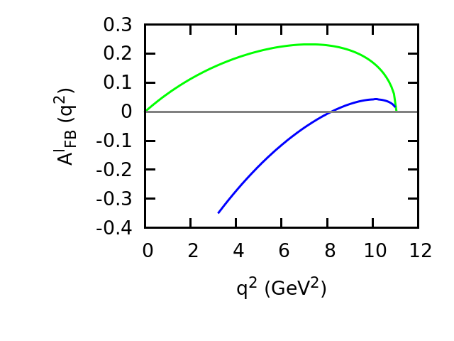
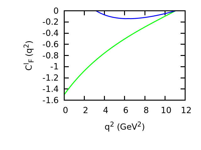
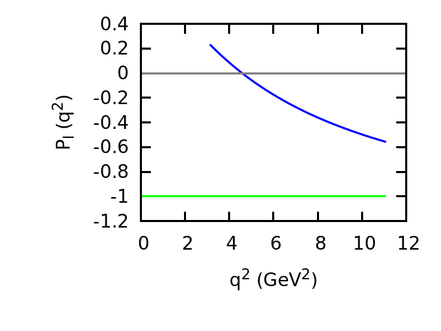
Figure 1: $q^{2}$ dependence of $A^{l}_{FB}(q^{2})$, $C_{F}^{l}(q^{2})$, and $P_{l}(q^{2})$ within the SM. Blue and green line corresponds to the $\tau$ and $e$ modes, respectively.

Now we proceed to discuss various NP scenarios. We want to see the effect of various NP couplings in a model independent way. In the first scenario, we assume that NP is coming from couplings associated with new vector type of interactions, i.e, from $V_{L}$ and $V_{R}$ only. We vary $V_{L}$ and $V_{R}$ while keeping $S_{L,\,R}=0$. In order to determine the allowed NP parameter space, we impose $1\sigma$ constraint coming from the measured values of the ratio of branching ratios $R_{D}$ and $R_{D^{\ast}}$. The allowed ranges in $V_{L}$ and $V_{R}$ that satisfies the $1\sigma$ experimental constraint are shown in the left panel of Fig. 2. In the right panel, we show the allowed ranges in $\mathcal{B}(B_{c}\to\tau\nu)$ and $\mathcal{B}(\Xi_{b}\to\Xi_{c}\tau\nu)$ obtained in this NP scenario. We see that $\mathcal{B}(B_{c}\to\tau\nu)$ obtained in this scenario is consistent with the $\mathcal{B}(B_{c}\to\tau\nu)\leq 5\%$ obtained in the SM. The corresponding ranges of all the observables are listed in Table. 4.

$\mathcal{B}(\Xi_{b}\to\Xi_{c}\tau\nu)\%$	$R_{\Xi_{c}}$	$<A_{FB}^{\tau}>$	$<C_{F}^{\tau}>$	$<P_{\tau}>$
$[2.36,\,3.71]$	$[0.254,\,0.410]$	$[-0.028,\,-0.346]$	$[-0.101,\,-0.113]$	$[-0.246,\,-0.333]$

Table 4: Ranges of various observables with $V_{L}$ and $V_{R}$ NP couplings.

We see a significant deviation from the SM prediction. Depending on the NP couplings $V_{L}$ and $V_{R}$, value of the observables can be either smaller or larger than the SM prediction.

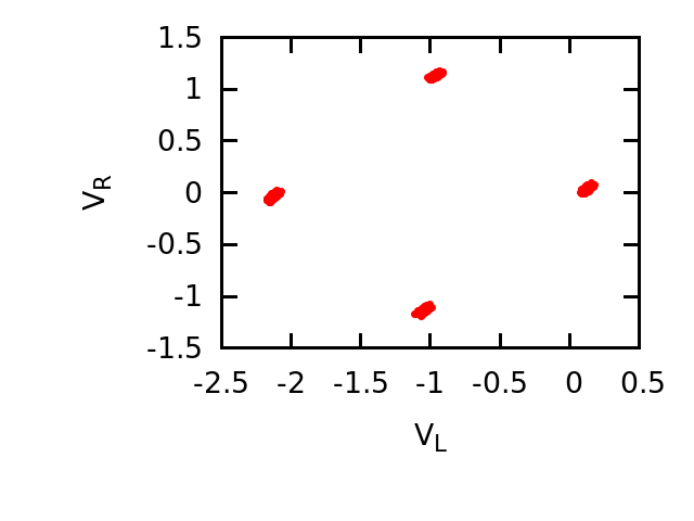
Figure 2: Allowed regions of $V_{L}$ and $V_{R}$ obtained using the $1\sigma$ constraint coming from $R_{D}$ and $R_{D^{\ast}}$ are shown in the left panel and the corresponding ranges in $\mathcal{B}(B_{c}\to\tau\nu)$ and $\mathcal{B}(\Xi_{b}\to\Xi_{c}\tau\nu)$ in the presence of these NP couplings are shown in the right panel.

We wish to look at the effect of the new physics couplings $(V_{L},\,V_{R})$ on different observables such as differential branching ratio ${\rm DBR}(q^{2})$, ratio of branching ratio $R(q^{2})$, forward backward asymmetry $A^{\tau}_{\rm FB}(q^{2})$, the convexity parameter $C_{F}^{\tau}(q^{2})$, and the $\tau$ polarization fraction $P_{\tau}(q^{2})$ for the $\Xi_{b}\to\Xi_{c}\tau\nu$ decays. In Fig. 3, we show in blue the allowed SM bands and in green the allowed bands of each observable once the NP couplings $V_{L}$ and $V_{R}$ are switched on. It can be seen that once NP is included the deviation from the SM expectation is quite large in case of ${\rm DBR}(q^{2})$, $R(q^{2})$, and $A^{\tau}_{\rm FB}(q^{2})$. However, the deviation is slightly less in case of $C_{F}^{\tau}(q^{2})$ and $P_{\tau}(q^{2})$. We observe that depending on the values of NP couplings, there may or may not be a zero crossing in the forward backward asymmetry parameter $A^{\tau}_{FB}(q^{2})$. In case of $P_{\tau}(q^{2})$, the zero crossing may shift towards the higher $q^{2}$ value than in the SM.

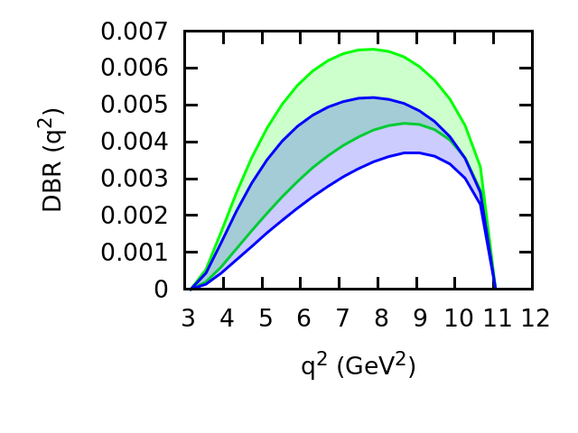
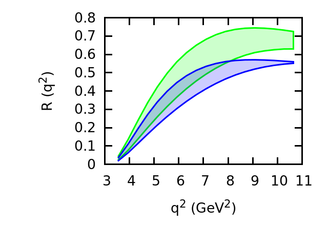
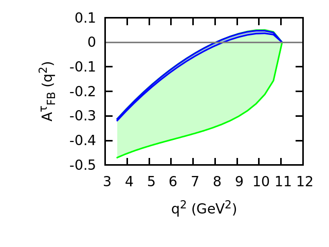
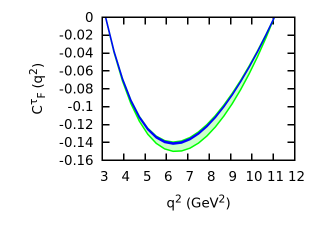
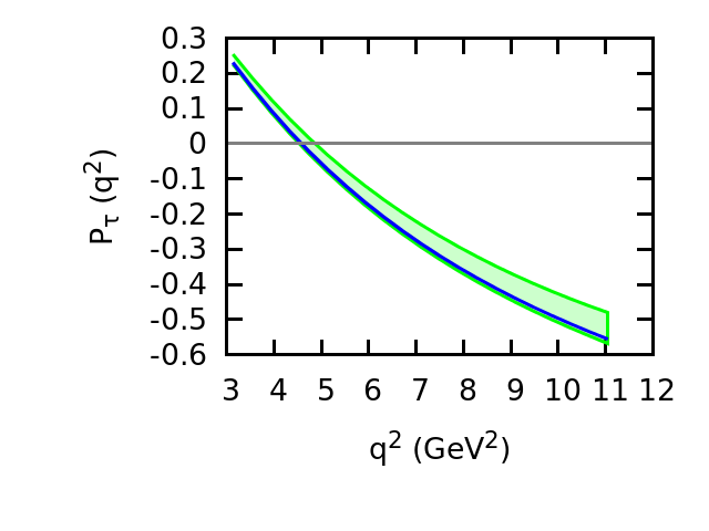
Figure 3: The dependence of the observables DBR$(q^{2})$, $R(q^{2})$, $A^{\tau}_{FB}(q^{2})$, $C_{F}^{\tau}(q^{2})$, and $P_{\tau}(q^{2})$ on $V_{L}$ and $V_{R}$ NP couplings. The allowed range in each observable is shown in light green band once the NP couplings $(V_{L},V_{R})$ are varied within the allowed ranges of the left panel of Fig. 2. The corresponding SM prediction is shown in light blue band.

In the second scenario, we assume that NP is coming from new scalar type of interactions, i.e, from $S_{L}$ and $S_{R}$ only. To explore the effect of NP coming from $S_{L}$ and $S_{R}$, we vary $S_{L}$ and $S_{R}$ and impose $1\sigma$ constraint coming from the measured values of $R_{D}$ and $R_{D^{\ast}}$. The resulting ranges in $S_{L}$ and $S_{R}$ obtained using the $1\sigma$ experimental constraint are shown in the left panel of Fig. 4. In the right panel of Fig. 4, the allowed ranges in $\mathcal{B}(B_{c}\to\tau\nu)$ and $\mathcal{B}(\Xi_{b}\to\Xi_{c}\,\tau\nu)$ are shown. We see that the branching ratio of $B_{c}\to\tau\nu$ obtained in this scenario is rather large, more than $30\%$. Even if we assume that $\mathcal{B}(B_{c}\to\tau\nu)$ can not be greater than $30\%$, then although $S_{L}$ and $S_{R}$ NP couplings can explain the anomalies present in $R_{D}$ and $R_{D^{\ast}}$, it, however, can not accommodate $B_{c}\to\tau\nu$ data. The allowed ranges in all the observables are reported in Table. 5. We see a significant deviation of all the observables from the SM prediction. It should be noted that the deviation observed in this scenario is more pronounced than the deviation observed with $V_{L}$ and $V_{R}$ NP couplings.

$\mathcal{B}(\Xi_{b}\to\Xi_{c}\tau\nu)$	$R_{\Xi_{c}}$	$<A_{FB}^{\tau}>$	$<C_{F}^{\tau}>$	$<P_{\tau}>$
$[1.94,\,5.42]$	$[0.200,\,0.616]$	$[-0.179,\,0.226]$	$[-0.052,\,-0.111]$	$[-0.371,\,0.338]$

Table 5: Ranges of various observables with $S_{L}$ and $S_{R}$ NP couplings.

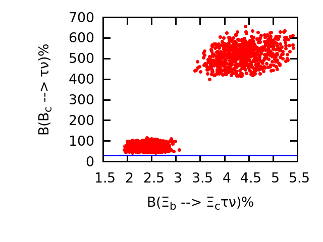
Figure 4: Allowed regions of $S_{L}$ and $S_{R}$ obtained using the $1\sigma$ constraint coming from $R_{D}$ and $R_{D^{\ast}}$ are shown in the left panel and the corresponding ranges in $\mathcal{B}(B_{c}\to\tau\nu)$ and $\mathcal{B}(\Xi_{b}\to\Xi_{c}\tau\nu)$ in the presence of these NP couplings are shown in the right panel. The blue horizontal line in the right panel corresponds to $\mathcal{B}(B_{c}\to\tau\nu)=30\%$.

We want to see the effect of these NP couplings on various $q^{2}$ dependent observables. In Fig. 5, we show how the observables ${\rm DBR}(q^{2})$, $R(q^{2})$, $A^{\tau}_{\rm FB}(q^{2})$, $C_{F}^{\tau}(q^{2})$, and $P_{\tau}(q^{2})$ behave as a function of $q^{2}$ with and without $S_{L}$ and $S_{R}$ NP couplings. The light blue band corresponds to the SM range whereas, the light green band corresponds to the range of the observable with $S_{L}$ and $S_{R}$ NP couplings. The deviations from the SM expectation is prominent in case of each observables. It should be mentioned that the deviation observed in this scenario is more pronounced than the deviation observed with $V_{L}$ and $V_{R}$ NP couplings. Depending on the values of $S_{L}$ and $S_{R}$ NP couplings, the zero crossing point of $A_{FB}^{\tau}(q^{2})$ and $P_{\tau}(q^{2})$ can be quite different from the SM prediction.

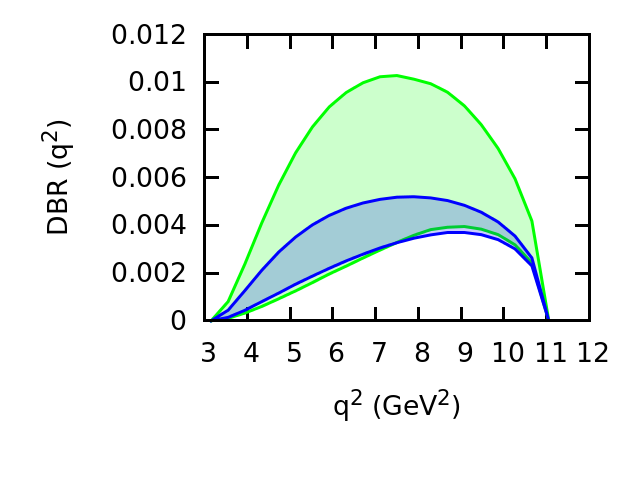
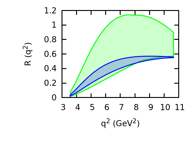
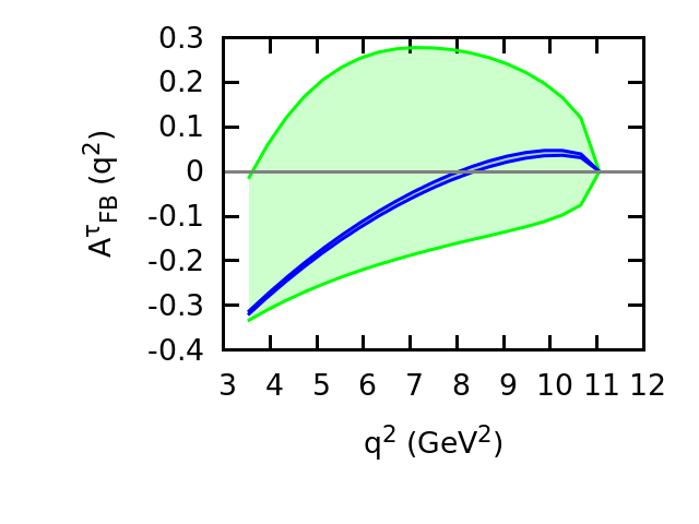
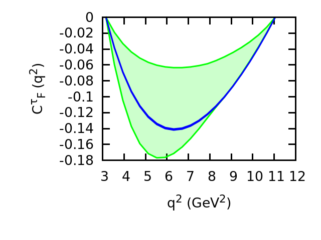
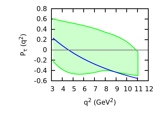
Figure 5: The dependence of the observables DBR$(q^{2})$, $R(q^{2})$, $A^{\tau}_{FB}(q^{2})$, $C_{F}^{\tau}(q^{2})$, and $P_{\tau}(q^{2})$ on $S_{L}$ and $S_{R}$ NP couplings. The allowed range in each observable is shown in light green band once the NP couplings $(S_{L},\,S_{R})$ are varied within the allowed ranges shown in the left panel of Fig. 4. The corresponding SM prediction is shown in light blue band.

IV Summary and conclusion

Lepton flavor universality violation has been reported in various semileptonic $B$ meson decays. Tensions between SM prediction and experiments exist in various semileptonic $B$ meson decays mediated via $b\to c$ charged current interactions and $b\to s\,l\,\bar{l}$ neutral current interactions. Study of $\Xi_{b}\to\Xi_{c}\,\tau\,\nu$ decays is important mainly for two reasons. First, it can act as a complimentary decay channel to $B\to(D,\,D^{\ast})\tau\nu$ decays mediated via $b\to c$ charged current interactions and, in principle, can provide new insights into the $R_{D}$ and $R_{D^{\ast}}$ anomaly. Second, precise determination of the branching fractions of this decay modes will allow an accurate determination of the CKM matrix element $|V_{cb}|$ with less theoretical uncertainty.

We have used the helicity formalism to study the $\Xi_{b}\to\Xi_{c}\,l\,\nu$ within the context of an effective Lagrangian in the presence of NP. We have defined various observables and provide predictions using form factors obtained in relativistic quark model. We have given the first prediction of various observables such as $R_{\Xi_{c}}$, $A^{l}_{FB}$, $P_{l}$, and $C_{F}^{l}$ for this decay mode. We also see the NP effects on various observables for this decay mode. Let us now summarize our main results.

We first report the central values and the $1\sigma$ ranges of all the observables for the $\Xi_{b}\to\Xi_{c}\,l\,\nu$ decays within the SM. The SM branching ratio of $\Xi_{b}\to\Xi_{c}\,l\,\nu$ decays is at the order of $10^{-2}$. We observe that the integrated quantities— forward backward asymmetry $<A^{l}_{FB}>$, longitudinal polarization fraction of lepton $<P_{l}>$, the convexity parameter $<C_{F}^{l}>$ change considerably while going from $e$ to the $\tau$ modes. There is even a sign change in case of the forward backward asymmetry parameter $<A^{l}_{FB}>$.

For the NP analysis, we include vector and scalar type of NP interactions and explore two different NP scenarios. In the first scenario, we consider only vector type of NP interactions, i.e, we consider that only $V_{L}$ and $V_{R}$ contributes to the decay mode. In the second scenario, we assume that NP is coming only from scalar type of interactions, i.e, from $S_{L}$ and $S_{R}$ only. The allowed ranges in the NP couplings are obtained by using $1\sigma$ constraint coming from the measured values of $R_{D}$ and $R_{D^{\ast}}$. We also study the effect of these NP couplings on various $q^{2}$ dependent observables such as ${\rm DBR}(q^{2})$, $R(q^{2})$, $A^{\tau}_{\rm FB}(q^{2})$, $C_{F}^{\tau}(q^{2})$, and $P_{\tau}(q^{2})$. We find significant deviations from the SM prediction once the NP couplings are included. However, the deviation from the SM prediction is more pronounced in case of scalar NP interactions $S_{L}$ and $S_{R}$. It should be mentioned that $\mathcal{B}(B_{c}\to\tau\nu)$ put a severe constraint on $S_{L}$ and $S_{R}$ NP couplings. However, the allowed range obtained for $\mathcal{B}(B_{c}\to\tau\nu)$ with $V_{L}$ and $V_{R}$ NP couplings is consistent with the $\mathcal{B}(B_{c}\to\tau\nu)\leq 5\%$ obtained in the SM.

Although, there is hint of NP in the meson sector, NP is not yet established. Study of $\Xi_{b}\to\Xi_{c}\,l\,\nu$ decays both theoretically and experimentally is well motivated because of the longstanding anomalies present in $R_{D}$ and $R_{D^{\ast}}$. It would be interesting to find out similar hint of NP in the semileptonic baryonic decays as well. At the same time, a precise measurement of $\mathcal{B}(\Xi_{b}\to\Xi_{c}\,l\,\nu)$ and a precise determination of $\Xi_{b}\to\Xi_{c}$ transition form factors will allow an accurate determination of the CKM matrix element $|V_{cb}|$.

References

- (1) http://www.slac.stanford.edu/xorg/hflav/semi/index.html
- (2) R. Aaij et al. [LHCb Collaboration], “Test of lepton universality using decays,” Phys. Rev. Lett. 113, 151601 (2014)
- (3) R. Aaij et al. [LHCb Collaboration], “Test of lepton universality with decays,” JHEP 1708, 055 (2017)
- (4) R. Aaij et al. [LHCb Collaboration], “Measurement of the ratio of branching fractions /,” arXiv:1711.05623 [hep-ex]
- (5) W. F. Wang, Y. Y. Fan and Z. J. Xiao, “Semileptonic decays in the perturbative QCD approach,” Chin. Phys. C 37, 093102 (2013)
- (6) R. Dutta and A. Bhol, “ semileptonic decays within the standard model and beyond,” Phys. Rev. D 96, no. 7, 076001 (2017)
- (7) M. A. Ivanov, J. G. Korner and P. Santorelli, “Semileptonic decays of mesons into charmonium states in a relativistic quark model,” Phys. Rev. D 71, 094006 (2005) Erratum: [Phys. Rev. D 75, 019901 (2007)] doi:10.1103/PhysRevD.75.019901, 10.1103/PhysRevD.71.094006 [hep-ph/0501051].
- (8) D. Ebert, R. N. Faustov and V. O. Galkin, “Semileptonic decays of heavy baryons in the relativistic quark model,” Phys. Rev. D 73, 094002 (2006) doi:10.1103/PhysRevD.73.094002 [hep-ph/0604017].
- (9) R. L. Singleton, “Semileptonic baryon decays with a heavy quark,” Phys. Rev. D 43, 2939 (1991). doi:10.1103/PhysRevD.43.2939
- (10) H. Y. Cheng and B. Tseng, “1/M corrections to baryonic form-factors in the quark model,” Phys. Rev. D 53, 1457 (1996) Erratum: [Phys. Rev. D 55, 1697 (1997)] doi:10.1103/PhysRevD.53.1457, 10.1103/PhysRevD.55.1697.2 [hep-ph/9502391].
- (11) M. A. Ivanov, V. E. Lyubovitskij, J. G. Korner and P. Kroll, “Heavy baryon transitions in a relativistic three quark model,” Phys. Rev. D 56, 348 (1997) doi:10.1103/PhysRevD.56.348 [hep-ph/9612463].
- (12) M. A. Ivanov, J. G. Korner, V. E. Lyubovitskij and A. G. Rusetsky, “Charm and bottom baryon decays in the Bethe-Salpeter approach: Heavy to heavy semileptonic transitions,” Phys. Rev. D 59, 074016 (1999) doi:10.1103/PhysRevD.59.074016 [hep-ph/9809254].
- (13) F. Cardarelli and S. Simula, “Analysis of the Lambda(b) —¿ Lambda(c) + lepton anti-neutrino(lepton) decay within a light front constituent quark model,” Phys. Rev. D 60, 074018 (1999) doi:10.1103/PhysRevD.60.074018 [hep-ph/9810414].
- (14) C. Albertus, E. Hernandez and J. Nieves, “Nonrelativistic constituent quark model and HQET combined study of semileptonic decays of Lambda(b) and Xi(b) baryons,” Phys. Rev. D 71, 014012 (2005) doi:10.1103/PhysRevD.71.014012 [nucl-th/0412006].
- (15) J. G. Korner, M. Kramer and D. Pirjol, “Heavy baryons,” Prog. Part. Nucl. Phys. 33, 787 (1994) doi:10.1016/0146-6410(94)90053-1 [hep-ph/9406359].
- (16) T. Bhattacharya, V. Cirigliano, S. D. Cohen, A. Filipuzzi, M. Gonzalez-Alonso, M. L. Graesser, R. Gupta and H. -W. Lin, “Probing Novel Scalar and Tensor Interactions from (Ultra)Cold Neutrons to the LHC,” Phys. Rev. D 85, 054512 (2012) [arXiv:1110.6448 [hep-ph]].
- (17) V. Cirigliano, J. Jenkins and M. Gonzalez-Alonso, “Semileptonic decays of light quarks beyond the Standard Model,” Nucl. Phys. B 830, 95 (2010) [arXiv:0908.1754 [hep-ph]].
- (18) T. Gutsche, M. A. Ivanov, J. G. Körner, V. E. Lyubovitskij, P. Santorelli and N. Habyl, “Semileptonic decay in the covariant confined quark model,” Phys. Rev. D 91, no. 7, 074001 (2015) [Phys. Rev. D 91, no. 11, 119907 (2015)] doi:10.1103/PhysRevD.91.074001, 10.1103/PhysRevD.91.119907 [arXiv:1502.04864 [hep-ph]].
- (19) T. Gutsche, M. A. Ivanov, J. G. Körner, V. E. Lyubovitskij and P. Santorelli, “Heavy-to-light semileptonic decays of and baryons in the covariant confined quark model,” Phys. Rev. D 90, no. 11, 114033 (2014) doi:10.1103/PhysRevD.90.114033 [arXiv:1410.6043 [hep-ph]].
- (20) J. G. Korner and G. A. Schuler, “Exclusive Semileptonic Heavy Meson Decays Including Lepton Mass Effects,” Z. Phys. C 46, 93 (1990).
- (21) S. Shivashankara, W. Wu and A. Datta, “ Decay in the Standard Model and with New Physics,” Phys. Rev. D 91, no. 11, 115003 (2015) doi:10.1103/PhysRevD.91.115003 [arXiv:1502.07230 [hep-ph]].
- (22) R. Dutta, “ decays within standard model and beyond,” Phys. Rev. D 93, no. 5, 054003 (2016) doi:10.1103/PhysRevD.93.054003 [arXiv:1512.04034 [hep-ph]].
- (23) C. Patrignani et al. [Particle Data Group], “Review of Particle Physics,” Chin. Phys. C 40, no. 10, 100001 (2016). doi:10.1088/1674-1137/40/10/100001