Refinements of Levenshtein bounds in $q$-ary Hamming spaces

Abstract.

We develop refinements of the Levenshtein bound in $q$-ary Hamming spaces by taking into account the discrete nature of the distances versus the continuous behavior of certain parameters used by Levenshtein. The first relevant cases are investigated in detail and new bounds are presented. In particular, we derive generalizations and $q$-ary analogs of a MacEliece bound. We provide evidence that our approach is as good as the complete linear programming and discuss how faster are our calculations. Finally, we present a table with parameters of codes which, if exist, would attain our bounds.

Dedicated to the memory of Professor Vladimir Levenshtein (1935-2017)

Keywords. Error-correcting codes, Levenshtein bound, bounds for codes.

1. Introduction

Let $Q=\{0,1,\ldots,q-1\}$ be the alphabet of $q$ symbols and $H(n,q)$ be the set of all $q$-ary vectors $x=(x_{1},x_{2},\ldots,x_{n})$ over $Q$. The Hamming distance $d(x,y)$ between points $x=(x_{1},x_{2},\ldots,x_{n})$ and $y=(y_{1},y_{2},\ldots,y_{n})$ from $H(n,q)$ is equal to the number of coordinates in which they differ. A non-empty set $C\subset H(n,q)$ is called a code. The investigation of the connections between the codelength $n$, cardinality $|C|$ and the minimum distance $d=d(C)=\min\{d(x,y),\ x\neq y\in C\}$ is of great importance in Coding Theory.

The spaces $H(n,q)$ are sometimes considered as polynomial metric spaces (cf. [9, 14, 16]), where using ”inner” products $\langle x,y\rangle:=1-\frac{2d(x,y)}{n}$ instead of distances is very convenient. We define $T_{n}=\{t_{0},t_{1},\ldots,t_{n}\}$, where $t_{i}:=-1+\frac{2i}{n}$, $i=0,1,\ldots,n$, as the set of all possible inner products.

Let $s\in T_{n}$ and

$$A_{q}(n,s):=\max\{|C|\colon C\subset H(n,q),s(C)\leq s\},$$

where $s(C)=\max\{\langle x,y\rangle,\ x\neq y\in C\}$, be the maximal possible cardinality of a code in $H(n,q)$ of prescribed maximal inner product $s$. In Coding Theory this quantity is usually denoted by $A_{q}(n,d)$, where $s=1-\frac{2d}{n}$ ($=t_{n-d}$) and $d$ is the minimum distance of $C$ (so we have replaced the condition $d(x,y)\geq d$ by $\langle x,y\rangle\leq s$).

Levenshtein (cf. [14, 15, 16], see also [9]) developed theory and proved universal upper bounds for $A_{q}(n,s)$. In this paper we describe refinements of the Levenshtein bound that can be applied for obtaining better bounds in the majority of the cases. Our refinements have two major advantages – they are easy to derive and allow analytic investigation to certain extent.

Improvements of the third Levenshtein bound in the binary case $q=2$ were obtained by Tietäväinen [25] and Krasikov-Litsyn [13], who developed bounds for $d=n-\frac{n+j}{2}$, where $0<j<\sqrt[3]{n}$. Earlier, in 1973, linear programming bounds were obtained by McEliece (unpublished, see [18, Chapter 17, Theorem 38]) who proved the asymptotic bound $A_{2}(n,s)\lesssim(n-j)(j+2)$, where $2d+j=n$ is as above, $s=1-\frac{2d}{n}$, and $j=o(\sqrt{n})$. The McEliece bound was improved in [25] and [13] for $j=o(n^{1/3})$.

On the other hand, binary codes of length $n=(2^{2m}+1)(2^{m}-1)$, size $M=2^{4m}$ and minimum distance $d=2^{2m-1}(2^{m}-1)$ (so $j=2^{m}-1$) were constructed by Sidel nikov [22]. This shows that the McEliece bound is of the correct order of magnitude. We also note that the maximum possible size of a code for $j=1$ and $n\equiv 1\pmod{4}$ is still unknown.

Much less is known in the $q$-ary case, where analogs of the Tietäväinen bound were obtained in [19]. Our results give a generalization of the McEliece bound – first as we prove it for every $n\geq q\geq 2$ and second, as we obtain its $q$-ary asymptotic analog.

This paper is organized as follows. In Section 2 we explain the general linear programming bound, the Levenshtein bound and related parameters. Section 3 is devoted to general description of our refinements and discussion on its limits. We develop the first relevant case giving a rigorous proof for the refinement of the third Levenshtein bound in Section 4, where we also investigate the asymptotics of the new bounds. We also provide evidence that our bounds for large enough $\frac{d}{n}=\frac{1-s}{2}$ are as good as the complete linear programming despite being considerably simpler. Asymptotic bounds from the refinement of the fourth Levenshtein bound are presented in Section 5. We also compile a table of feasible parameters for good codes attaining our bounds.

2. Preliminaries

2.1. Krawtchouk polynomials and the linear programming framework

For fixed $n$ and $q$, the (normalized) Krawtchouk polynomials are defined by

$$Q_{i}^{(n,q)}(t):=\frac{1}{r_{i}}K_{i}^{(n,q)}(d),$$

where $d=\frac{n(1-t)}{2}$, $r_{i}=(q-1)^{i}{n\choose i}$, and $K_{i}^{(n,q)}(d)=\sum_{j=0}^{i}(-1)^{j}(q-1)^{i-j}\binom{d}{j}\binom{n-d}{i-j}$ are the (usual) Krawtchouk polynomials that obey the three-term recurrent relation

$$K_{0}^{(n,q)}(d)=1,\ \ K_{1}^{(n,q)}(d)=n(q-1)-qd,$$

$$K_{i+1}^{(n,q)}(d)=\frac{i+(q-1)(n-i)-qd}{i+1}K_{i}^{(n,q)}(d)-\frac{(q-1)(n-i+1)}{i+1}K_{i-1}^{(n,q)}(d),\mbox{ for }i\geq 1.$$

We point out that even if the Krawtchouk polynomials $K_{i}^{(n,q)}(d)$ are defined for all non-negative integers $i$, the normalized polynomials $Q_{i}^{(n,q)}(t)$ are only defined for integers $i\in[0,n]$. If $f(t)\in\mathbb{R}[t]$ is a real polynomial of degree $m\geq 0$, then $f(t)$ can be uniquely expanded in terms of the Krawtchouk polynomials as $f(t)=\sum_{i=0}^{m}f_{i}Q_{i}^{(n,q)}(t)$.

The next (folklore) assertion is the main source of linear programming bounds (aka Delsarte bounds) for $A_{q}(n,s)$.

Theorem 2.1.

Let $n\geq 2$ and $s\in[-1,1)$ be fixed and $f(t)$ be a real polynomial of degree $m$ such that:

(A1) $f(t)\leq 0$ for every $t\in T_{n}\cap[-1,s]$;

(A2) the coefficients in the Krawtchouk expansion $f(t)=\sum_{i=0}^{m}f_{i}Q_{i}^{(n,q)}(t)$ satisfy $f_{i}\geq 0$ for every $i$.

Then $A_{q}(n,s)\leq\frac{f(1)}{f_{0}}$.

2.2. The Levenshtein bound

The so-called adjacent polynomials as introduced by Levenshtein (cf. [16, Section 6.2], see also [14, 15]) are given by

(1) $$Q_{i}^{(1,0,n,q)}(t)=\frac{K_{i}^{(n-1,q)}(d-1)}{\sum_{j=0}^{i}{n\choose j}(q-1)^{j}},\ \ Q_{i}^{(1,1,n,q)}(t)=\frac{K_{i}^{(n-2,q)}(d-1)}{\sum_{j=0}^{i}{n-1\choose j}(q-1)^{j}},$$

$$Q_{i}^{(0,1,n,q)}(t)=\frac{K_{i}^{(n-1,q)}(d)}{{n-1\choose i}(q-1)^{i}},$$

where $d=n(1-t)/2$.

For $a\in\{0,1\}$ and $i\in\{1,2,\ldots,n-1\}$, denote by $t_{i}^{1,a}$ the greatest zero of the adjacent polynomial $Q_{i}^{(1,a,n,q)}(t)$ (see (1)) and also define $t_{0}^{1,1}=-1$ as well as $t_{n}^{1,0}=1$. We have the interlacing properties $t_{k-1}^{1,1}<t_{k}^{1,0}<t_{k}^{1,1}$, see [16, Lemmas 5.29, 5.30]. For a positive integer $m=2k-1+\varepsilon$, $\varepsilon\in\{0,1\}$, let

$$\mathcal{I}_{m}:=\left[t_{k-1+\varepsilon}^{1,1-\varepsilon},t_{k}^{1,\varepsilon}\right).$$

Then the set of well defined intervals $\left\{\mathcal{I}_{m}\right\}_{m=1}^{2n-1}$ forms a partition of the interval $[-1,1)$ into non-overlapping subintervals. For every $s\in\mathcal{I}_{m}$, Levenshtein used Theorem 2.1 with certain polynomials of degree $m$

(2) $$f_{m}^{(n,s,q)}(t)=(t-s)(t+1)^{\varepsilon}A^{2}(t)$$

(see [16, Equations (5.81) and (5.82)]), where $\deg(f_{m}^{(n,s)})=m$, to obtain (see [16, Equations (6.45) and (6.46)])

(3) $$A_{q}(n,s)\leq L_{m}(n,s;q)=q^{1-\varepsilon}\left(1-\frac{Q_{k-1}^{(1,1-\varepsilon,n,q)}(s)}{Q_{k}^{(0,\varepsilon,n,q)}(s)}\right)\sum\limits_{j=0}^{k-1+\varepsilon}{n\choose j}(q-1)^{j}$$

for every $s\in\mathcal{I}_{m}$. The bound (3) is attained by many codes with good combinatorial properties but is weak in many other particular cases. It is also worth to mention its good asymptotic behavior (see [3], [16, Section 6.2]).

In [6] two of the authors obtained (for any $q$) and investigated (for $q=2$) necessary and sufficient conditions for global optimality of the Levenshtein bounds (see also [16, Theorem 5.47]). Here we discuss another possibility of improving Levenshtein bounds by taking into account the discrete nature of the set of inner products.

3. Our refinement – vanishing at inner products instead of zeros of the Levenshtein’s polynomial

The roots $-1\leq\alpha_{0}<\alpha_{1}<\cdots<\alpha_{k-2+\varepsilon}<\alpha_{k-1+\varepsilon}=s$ of the Levenshtein polynomials $f_{m}^{(n,s,q)}(t)$ (we recall that $m=2k-1+\varepsilon$, $\varepsilon\in\{0,1\}$) are exactly the roots of the equation

(4) $$(t+1)^{\varepsilon}[P_{k}(t)P_{k-1}(s)-P_{k}(s)P_{k-1}(t)]=0,$$

where $P_{i}(t)=Q_{i}^{(1,\varepsilon,n,q)}(t)\in\mathbb{Q}[t]$. Since (4) is equivalent to an equation with integer coefficients, the double zeros $\alpha_{i}$, $i=\varepsilon,\ldots,k-2+\varepsilon$, will rarely coincide exactly with inner products from the set $T_{n}$. Taking this into account we obtain the following refinement of the Levenshtein bound.

We first locate the nodes $\alpha_{i}$, $i=\varepsilon,\ldots,k-2+\varepsilon$, with respect to the elements (the inner products) of $T_{n}$. Then, if $\alpha_{i}\in(t_{j-1},t_{j})$ for some integer $j\in[1,n]$, we replace the double zero $\alpha_{i}$ by two simple zeros $\gamma_{2(i-\varepsilon)+1}=t_{j-1}$ and $\gamma_{2(i-\varepsilon+1)}=t_{j}$. After setting $\gamma_{2k-1}=s$, we define the polynomial

$$f(t)=(t+1)^{\varepsilon}\prod_{i=1}^{2k-1}(t-\gamma_{i})$$

of degree $m=2k-1+\varepsilon$. We observe that the values of this polynomial in the interval $(t_{j-1},t_{j})$ are positive and, in particular, $f(\alpha_{i})\geq 0$, with (very rare apart from $\alpha_{k-1+\varepsilon}=s\in T_{n}$) equality case if and only if $\alpha_{i}=t_{j}$. Finally, in the case when the degree $m$ exceeds the codelength $n$ we reduce the polynomial $f(t)$ to its remainder from its division by $\displaystyle g(t)=\prod_{i=0}^{n}(t-t_{i})$. This operation is standard when the polynomial metric space (PMS) is finite.

This construction clearly implies that the condition (A1) is satisfied. Moreover, using the quadrature formula

(5) $$f_{0}=\frac{1}{L_{m}(n,s;q)}+\sum_{i=0}^{k-1+\varepsilon}\rho_{i}f(\alpha_{i})$$

(see [16, Theorem 5.39]) and the inequalities $f(\alpha_{i})\geq 0$ we conclude that $f_{0}>0$ always follows.

The condition (A2) for $i\geq 1$ can be easily checked numerically in every particular case, and it is satisfied in the great majority of the cases we considered. We give a rigorous proof for the case $m=3$ below.

Summarizing, whenever we have (A2), Theorem 2.1 gives upper bound for the corresponding $A_{q}(n,s)$. Clearly, this is a strict improvement of the Levenshtein bound (3) if and only if $\alpha_{i}\not\in T_{n}$ for at least one $i$. Note that $\alpha_{i}\in T_{n}$ occurs very rare – this is connected to integral zeros of Krawtchouk polynomials (see [12, 23]).

Our numerical results cover wide range of values of $q$, $n$ and $s$, as we inspect all feasible $s$ for given $q$ and $n$. Unfortunately, comparisons with well established sources such as [7, 1, 4] can be made in small range, namely, for alphabet size $q=2$, 3, 4, and 5, and for lengths $n\leq 28$, $n\leq 16$, $n\leq 12$, and $n\leq 11$, respectively. In these ranges we recover the following best known upper bounds

$$A_{3}(14,-1/7)\leq 237,\ \ A_{4}(11,-3/11)\leq 320,\ \ A_{5}(11,-5/11)\leq 250$$

(the Levenshtein bounds are 256.5, 364, and 265, respectively).

It is clear that, in every particular case, the numerics from our refinements can not be better than the complete (integer) linear programming (see, for example [26]). However, we are going to show strong evidence that for every fixed $m$, our method gives the same results as the complete linear programming gives for large enough $n$ despite being considerably simpler for computation.

The much easier computation allows us to go for large lengths. Bounds for large lengths were numerically investigated (for binary codes only) by Barg-Jaffe [2]. Our computational results agree well with their application of the simplex method for large $\frac{d}{n}=\frac{1-s}{2}$. We give a short table for comparison. The bounds are computed for $\frac{1}{n}\log_{2}A_{2}(n,s)$.

Table 1. Bounds for binary codes, $n=1000$, $\frac{d}{n}=\frac{1-s}{2}\in[0.25,0.45]$.

$d/n$	0.25	0.3	0.35	0.4	0.45
$L_{m}(n,s;2)$	0.387	0.283	0.191	0.115	0.505
our bound	0.386	0.281	0.188	0.110	0.047
simplex from [2]	0.380	0.280	0.188	0.109	0.047

This comparison and our computational results for larger $q$ lead us to the conjecture that our method matches the best results possible by Theorem 2.1 for large enough ratio $d/n=(1-s)/2$.

Conjecture 3.1.

For a fixed $q\geq 3$ there exist a constant $s_{q}$ such that whenever $s\in[-1,s_{q})\cap T_{n}$ (that is large enough $d/n=(1-s)/2$) the above refinements are the best that can be obtained by Theorem 2.1.

In order to support this conjecture, in Figure 1 we present graph for the function $s_{q}(n)$ defined as the range $[-1,s_{q}(n))\cap T_{n}$ where our improvement is optimal in the sence of Theorem 2.1.

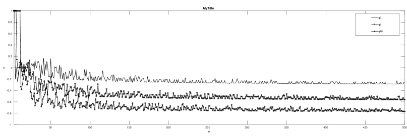
Figure 1. The function $s_{q}(n)$ for some $q$’s and codelengths $n\in[3,500]$.

We note also that, similarly to [2], our computations do not support the conjecture of Samorodnitsky [20] on the exponential strength of the linear programming method.

Semidefinite programming was shown to be better than the linear programming in most particular cases (see, for example, [10, 21, 17]) but it hardly gives bounds in analytic forms. So we see another advantage in giving analytic form of our bounds in the first cases (see the next sections).

4. The refinement of $L_{3}(n,s;q)$

In this section we apply our refinement in the case of the third Levenshtein bound. We provide proof for the feasibility of the chosen polynomial as well as some numerical results for the global optimality of this polynomial.

4.1. Proof of the feasibility of suggested polynomial

Let us set

(6) $$d=n-1-\frac{n-2+j}{q},$$

where the parameter $j$ will be explained below. We proceed with the general case of upper-bounding $A_{q}(n,s)$ in the range

$$s\in\mathcal{I}_{3}=\left[t_{1}^{1,1},t_{2}^{1,0}\right)=\left[-\frac{(q-2)(n-2)}{nq},-\frac{(q-2)(n-2)}{nq}+\frac{S_{1}-q}{nq}\right),$$

where $S_{1}=\sqrt{q^{2}+4(q-1)(n-2)}$. Since $d=n(1-s)/2$, we obtain the ranges for $d$ and $j$ to be

(7) $$d\in\left((n-1)-\frac{n-2}{q}-\frac{S_{1}-q}{2q},(n-1)-\frac{n-2}{q}\,\right]\iff j\in\mathcal{J}_{3}=\left[0,\frac{S_{1}-q}{2}\right).$$

The simple form of $\mathcal{J}_{3}$ justifies the change of the variable.

In the particular case of $m=3$ the polynomial defined in (2) becomes

$$f_{3}^{(n,s,q)}(t)=(t-\alpha_{0})^{2}(t-s)=(t-\alpha_{0})^{2}(t-\alpha_{1})\,,$$

where $s=\alpha_{1}=1-\frac{2d}{n}=-1+\frac{2(n-2+j+q)}{nq}$ and $\alpha_{0}=-1+\frac{2j(n-1)}{nq(j+q-1)}$, since $\alpha_{0}$ and $s$ are the roots of the equation (4) for $k=2$ and $\varepsilon=0$. Let us set $d_{0}=\frac{n(1-\alpha_{0})}{2}=n-\frac{j(n-1)}{q(j+q-1)}$ and define $e$ to be the unique rational number in the interval $(0,1]$ such that $d_{0}+e$ is integer. We point out that

$$\alpha_{0}\in\left(1-\frac{2(d_{0}+e)}{n},1-\frac{2(d_{0}+e-1)}{n}\,\right]$$

and that $e=\frac{r}{q(j+q-1)}$, where $r$ is the positive remainder from the division of $j(n-1)$ by $q(j+q-1)$, i.e. $r\equiv j(n-1)\pmod{q(j+q-1)}$ and $r\in\left(0,q(j+q-1)\right]\cap\mathbb{Z}$.

Now we are in a position to define our improving polynomial as

(8) $$\begin{array}[]{rcl}f(t)&=&\left(t-1+\frac{2(d_{0}+e)}{n}\right)\left(t-1+\frac{2(d_{0}+e-1)}{n}\right)(t-s)\\ &=&\left(t+1+\frac{2e}{n}-\frac{2j(n-1)}{nq(j+q-1)}\right)\left(t+1+\frac{2(e-1)}{n}-\frac{2j(n-1)}{nq(j+q-1)}\right)\times\\ &&\left(t+1-\frac{2(n-2+j+q)}{nq}\right)\\ &=&f_{0}+f_{1}Q_{1}^{(n,q)}(t)+f_{2}Q_{2}^{(n,q)}(t)+f_{3}Q_{3}^{(n,q)}(t),\end{array}$$

where the coefficients $f_{i}$, $i=3,2,1,0$, are given by

$$f_{3} = \frac{8(q-1)^{3}(n-2)(n-1)}{q^{3}n^{2}}>0,$$

(9) $$f_{2} = \frac{8(q-1)^{2}(n-1)A}{q^{3}n^{2}(q+j-1)},$$

(10) $$f_{1} = \frac{8(q-1)\left((eq-B)^{2}+C\right)}{q^{3}n^{2}},$$

$$f_{0} = \frac{8\left(a^{2}(2-q-j)+Da+E\right)}{q^{3}n^{3}}>0,$$

for

$$A = -j^{2}+(2eq-1)j+(q-1)(2n+2eq+q-4),$$

$$B = \frac{1}{j+q-1}\left[j(j-2)-n(q-1)+\frac{q}{2}(3j+q-1)\right],$$

$$C = -j^{2}+(-q+2)j+(3n-2)(q-1)-\frac{q^{2}}{4},$$

$$D = (j+q-1)[2n(q-1)-q]+q,$$

$$E = -n(n-1)(q-1)^{2}(j+q),$$

$$a = \frac{(n-1)(q-1)(q+j)}{q+j-1}+eq.$$

We proceed with the proof of the positivity of the coefficients $f_{1}$ and $f_{2}$.

Lemma 4.1.

We have $f_{2}>0$ for every $n\geq 2$ and $q\geq 2$.

Proof.

It follows from (9) that it is enough to prove that $A>0$. Observing that $A$ is a concave quadratic function in $j$, according to (7) we have to check the positivity of $A$ for $j=0$ and $j=\frac{S_{1}-q}{2}$, respectively. For the former we have

$$A=(q-1)(2n+2eq+q-4)\geq(q-1)(2n+q-4)>0$$

and for the latter

$$A=\left(eq+\frac{q-1}{2}\right)S_{1}+eq(q-2)+\frac{(2n+q-4)(q-1)}{2}>0,$$

whenever $n\geq 2$ and $q\geq 2$. ∎

Lemma 4.2.

We have $f_{1}>0$ for every $n\geq q\geq 2$.

Proof.

According to (10) it is sufficient to show that $C>0$. As in the proof of Lemma 4.1, we observe that $C$ is a concave quadratic function of $j$ so we check its values at the limits of the interval $\mathcal{J}_{3}$. We obtain those to be

$$(3n-2)(q-1)-\frac{q^{2}}{4}\geq(3q-2)(q-1)-\frac{q^{2}}{4}=2+\frac{q}{4}(11q-20)>0$$

and

$$S_{1}+2n(q-1)-q-q^{2}/4\geq S_{1}+\frac{q}{4}(7q-12)>0,$$

whenever $n\geq q\geq 2$. ∎

Remark 4.3.

Our numerics suggest that we might always have $f_{2}>f_{1}>f_{0}$. Since $f_{0}>0$ follows by the formula (5), another proof of the positivity of $f_{1}$ and $f_{2}$ could probably be done along these lines.

Theorem 4.4.

We have

(11) $$A_{q}(n,s)\leq\frac{a(a+q)dq}{a^{2}(2-q-j)+Da+E},$$

where the parameters are determined as above.

Proof.

The condition (A1) is obviously satisfied by our improving polynomial. The condition (A2) is satisfied as well – Lemmas 4.1 and 4.2 give $f_{2}\geq 0$ and $f_{1}\geq 0$, respectively, $f_{3}>0$ is obvious, and $f_{0}>0$ follows, as mentioned above, from (5). Therefore $A_{q}(n,s)\leq\frac{f(1)}{f_{0}}$ and simplifications give the desired bound. ∎

Example 4.5.

For $q=4$, $n=11$ and $s=-3/11$ (this $s$ corresponds to minimum distance $d=n(1-s)/2=7$) we are in the range of the third Levenshtein bound $L_{3}(11,s;4)$. Since $\alpha_{0}=-\frac{17}{22}\in\left(-\frac{9}{11},-\frac{7}{11}\right)$ and $\alpha_{1}=s=-\frac{3}{11}$, we have our improving polynomial as follows:

$$f(t) = \left(t+\frac{9}{11}\right)\left(t+\frac{7}{11}\right)\left(t+\frac{3}{11}\right)$$

$$= \frac{63}{5324}Q_{0}^{(11,4)}(t)+\frac{117}{484}Q_{1}^{(11,4)}(t)+\frac{45}{44}Q_{2}^{(11,4)}(t)+\frac{1215}{484}Q_{3}^{(11,4)}(t)$$

and $A_{4}(11,-3/11)\leq\frac{f(1)}{f_{0}}=320$ (here $L_{3}(11,-3/11;4)=364$). The best known lower bound in this case is $A_{4}(11,-3/11)\geq 128$ (see [7]). Further analysis via the distance distributions of a putative quaternary $(11,320,-3/11)$ code $C$ does not give a contradiction. Indeed, all possible inner products of $C$ are $-\frac{3}{11}$, $-\frac{7}{11}$ and $-\frac{9}{11}$ and such a code must be distance regular, i.e. every point of $C$ has the same distance distribution, which turns out to be integral.

We now calculate the asymptotic form of the bound from Theorem 4.4.

Corollary 4.6.

Let $j=cn^{\alpha}\in\mathcal{J}_{3}$ for some positive constant $c$ and some $\alpha\in[0,1/2]$. The behavior of the upper bound given by (11) as $n\to\infty$ is as follows

(12) $$A_{q}(n,s)\leq[(q-1)n-(j+q-2)](j+q)+j(j+q-1)^{2}+o(1),\ \alpha\in[0,1/5),$$

(13) $$A_{q}(n,s)\leq(q-1)(q+j)n+j^{3}+\frac{c^{5}n^{5\alpha-1}}{q-1}+o(n),\ \alpha\in[1/5,1/2),$$

and

(14) $$A_{q}(n,s)\leq\frac{c(q-1)^{2}}{q-1-c^{2}}n^{3/2}+\frac{(q-1)(c^{4}-(q-1)(3c^{2}-q^{2}+q))}{(q-1-c^{2})^{2}}n+o(n),\ \alpha=1/2.$$

Proof.

The upper bound in (11) can be re-written as

(15) $$\begin{array}[]{lcl}A_{q}(n,s)&\leq&[(q-1)n-(j+q-2)](j+q)+j(j+q-1)^{2}\\ &&+\displaystyle\frac{[(q-1)n+(eq+1)(eq+1-q)]j^{6}+P_{q,e,n}(j)}{(q-1)^{2}(j+q)n^{2}+Q_{q,e,n}(j)},\end{array}$$

where $P_{q,e,n}(j)$ and $Q_{q,e,n}(j)$ are polynomials in $j$ of degrees $5$ and $3$, respectively, and with coefficients that are linear in $n$. We notice that for the fraction in (15), the nominator is of order $\Theta(n^{1+6\alpha})$ and that the denominator has the order $\Theta(n^{2+\alpha})$ for all $\alpha\in[0,1/2]$. This gives the result in (12) since $1+6\alpha<2+\alpha$ when $\alpha\in[0,1/5)$.

To obtain (13), we observe that for large $n$ the nominator behaves like $(q-1)nj^{6}+\Theta(n^{1+5\alpha})$. For all $\alpha\in[1/5,1/2)$ we have $1+5\alpha-(2+\alpha)<1$ and also $i\alpha<1$, for $i=0,1,2$. Now (13) follows by ignoring the terms of orders in $n$ that are less than $1$.

Finally, by substituting $j=c\sqrt{n}$ in (15) and performing polynomial division for the polynomials in the variable $x=\sqrt{n}$ we arrive at (14). ∎

4.2. On Conjecture 3.1 for $m=3$

We reformulate the linear programming bound back to its classical form (see [8, Sections 3.2 and 3.3], [9, Section 3B], [15, Corollary 2.7]).

Theorem 4.7.

Let the polynomial $g(z)=\sum_{i=0}^{n}g_{i}K_{i}^{(n,q)}(z)$ satisfies the conditions

$$g_{0}>0,\ g_{i}\geq 0,\ i=1,2,\ldots,n;$$

$$g(0)>0,\ g(i)\leq 0,\ i=d,d+1,\ldots,n.$$

Then $A_{q}(n,s)\leq g(0)/g_{0}$, where $s=1-2d/n$.

In the light on Theorem 4.7 the best upper bound on the quantity $A_{q}(n,s)$ is obtained by the polynomial $g^{*}(z)=1+\sum_{i=1}^{n}\frac{x_{i}^{*}}{r_{i}}K_{i}^{(n,q)}(z)=1+\sum_{i=1}^{n}\frac{K_{i}^{(n,q)}(z)}{(q-1)^{i}{n\choose i}}x_{i}^{*}$ for which the coefficients $\overline{x}^{*}=(x_{1}^{*},x_{2}^{*},\cdots,x_{n}^{*})$ constitute a solution to the linear optimization problem

(16) $$\begin{array}[]{lrll}\text{minimize}\displaystyle&x_{1}+x_{2}+\cdots+x_{n}&&\\ \text{subject to}&\displaystyle\sum_{l=1}^{n}\frac{K_{l}^{(n,q)}(i)}{r_{l}}\!\!\!&x_{l}\leq-1,&i=d,(d+1),\dots,n\\ &&x_{l}\geq 0,&l=1,2,\dots,n.\end{array}$$

Applying the KKT optimality conditions (see for example [5, Section 5.5]) we can conclude that necessary and sufficient condition for $\overline{x}^{*}$ to be optimal is the existence of numbers $\lambda_{l},\,l=1,2,\dots,n$, and $\mu_{i},\,i=d,d+1,\dots,n$, such that

(17) $$\begin{array}[]{rcll}\lambda_{l}&=&\displaystyle 1+\sum_{i=d}^{n}\mu_{i}\frac{K_{l}^{(n,q)}(i)}{r_{l}}\geq 0,&l=1,2,\dots,n,\\ \lambda_{l}x_{l}^{*}&=&0,&l=1,2,\dots,n,\\ \mu_{i}g^{*}(i)&=&0,&i=d,(d+1),\dots,n,\\ \mu_{i}&\geq&0,&i=d,(d+1),\dots,n.\end{array}$$

Equation (17) turns out to be a very powerful tool for checking the global optimality of a given polynomial. In particular, if we have a polynomial $f(t)$ of degree $m$ that satisfies conditions (A1) and (A2) of Theorem 2.1 and has $m$ different roots in the interval $[-1,s]$, then we can exactly determine the numbers $\mu_{i},\,i=d,d+1,\dots,n$, if the Krawtchouk expansion of $f(t)$ in (A2) has strictly positive coefficients. The polynomial $f(t)$ would then be globally optimal if and only if all the lambdas, $\lambda_{l},\,l=1,2,\dots,n$, calculated as in (17) are non-negative. Our approach for improving the Levenshtein bound very often results in such polynomials.

Let us now consider the polynomial $f(t)$ as defined by (8) and let us set $g(z)=\frac{1}{f_{0}}f\left(1-\frac{2z}{n}\right)$. We can easily verify that

(18) $$g(z)=1+\sum_{i=1}^{3}\frac{f_{i}}{f_{0}}\frac{K_{i}^{(n,q)}(z)}{r_{i}}.$$

We now determine the Lagrange multipliers $\lambda_{i}^{*}$ and $\mu_{i}^{*}$ for the polynomial defined in (18). It has already been shown that $f_{i}>0,\,i=0,1,2,3$, which according to (17) means that $\lambda_{i}^{*}=0,\,i=1,2,3$. Since $g(i)=0$ only for $i\in\{d,d_{0}+e-1,d_{0}+e\}$ we have $\mu_{i}^{*}=0$ for all $i\in\{d+1,d+2,\dots,n\}\setminus\{d_{0}+e-1,d_{0}+e\}$. The remaining three $\mu_{i}^{*}$’s can be obtained from the system of linear equations

(19) $$\mu_{d}^{*}\frac{K_{l}^{(n,q)}(d)}{r_{l}}+\mu_{d_{0}+e-1}^{*}\frac{K_{l}^{(n,q)}(d_{0}+e-1)}{r_{l}}+\mu_{d_{0}+e}^{*}\frac{K_{l}^{(n,q)}(d_{0}+e)}{r_{l}}=-1,\,l=1,2,3.$$

The system (19) has an unique solution $(\mu_{d}^{*},\mu_{d_{0}+e-1}^{*},\mu_{d_{0}+e}^{*})$ with help of which we can calculate the remaining $\lambda_{i}^{*}$, for $i=4,5,\dots,n$, according to

(20) $$\lambda_{i}^{*}=1+\mu_{d}^{*}\frac{K_{i}^{(n,q)}(d)}{r_{i}}+\mu_{d_{0}+e-1}^{*}\frac{K_{i}^{(n,q)}(d_{0}+e-1)}{r_{i}}+\mu_{d_{0}+e}^{*}\frac{K_{i}^{(n,q)}(d_{0}+e)}{r_{i}}.$$

The first step towards the calculation of the lambdas is the following statement.

Lemma 4.8.

The weights $(\mu_{d}^{*},\mu_{d_{0}+e-1}^{*},\mu_{d_{0}+e}^{*})$ that solve system (19) can be calculated as

$$\mu_{d}^{*} = \frac{n(q-1)CD[C+q(j+q-1)]}{AB[B+q(j+q-1)]},$$

$$\mu_{d_{0}+e-1}^{*} = \frac{en(q-1)E[C+q(j+q-1)]}{AB},$$

$$\mu_{d_{0}+e}^{*} = \frac{(1-e)n(q-1)CE}{A[B+q(j+q-1)]},$$

where

$$A = -(q+j-2)[eq(j+q-1)]^{2}+(n-1)(q-1)(j+q)[n(q-1)-j(q+j-2)]$$

$$+eq(j+q-1)[(q^{2}+jq-q-2j)(q+j-2)+2n(q-1)],$$

$$B = (n-2+j)(q-1)+j(j-1)+eq(j+q-1),$$

$$C = (n-1)(q-1)(j+q)+eq(j+q-1),$$

$$D = \left[(n-1)(q-1)+(2e-1)(j+q-1)\frac{q}{2}\right]^{2}+(j+q-1)^{2}\left[(n-1)(q-1)-\frac{q^{2}}{4}\right],$$

$$E = (j+q-1)^{3}[(n-1)(q-2)+n-j].$$

Proof.

Direct check shows that the above defined $\mu_{d}^{*},\mu_{d_{0}+e-1}^{*}$ and $\mu_{d_{0}+e}^{*}$ satisfy (19) for any $n$, $q$, $e\in(0,1]$, $j\in\mathcal{J}_{3}$ and $l=1,2,3$. ∎

The non-negativity of $\mu_{d}^{*},\mu_{d_{0}+e-1}^{*}$ and $\mu_{d_{0}+e}^{*}$ for $n\geq q\geq 2$, $j\in\mathcal{J}_{3}$ and any $e\in[0,1)$ can be derived from Lemma 4.8 by showing the positivity of the parameters $A,B,C,D$ and $E$. Obviously $B>0$ and $C>0$ with the only exception of the trivial case $n=q=2$, $e=j=0$ for which $B=0$. The parameter $D$ is positive since $(n-1)(q-1)\geq(q-1)^{2}\geq(q/2)^{2}$ whenever $n\geq q\geq 2$ with equality only for $n=q=2$. As $A$ is a quadratic function in $e$ with negative leading coefficient, its positivity for $e\in[0,1)$ can be checked by investigating the values for $e=0$ and $e=1$. For these values we have $(n-1)(q-1)(j+q)[n(q-1)-j(q+j-2)]$ and $[(n(q-1)+q+1)j+(n+1)q(q-1)][n(q-1)-j(q+j-2)]$, respectively. For any $j\in\mathcal{J}_{3}$ we have

$$n(q-1)-j(q+j-2)\geq n(q-1)-\frac{S_{1}-q}{2}(q+\frac{S_{1}-q}{2}-2)=(q-2)+S_{1}>0,$$

which shows the positivity of $A$. Finally, the positivity of $E$ follows from the fact that $(n-1)(q-2)+n>(S_{1}-q)/2\geq j$.

We summarize the above observations into the following result.

Theorem 4.9.

Let $f(t)$ be the third degree polynomial given in (8) and let $\lambda_{i}^{*}$, for $i=4,5,\dots,n$, be given by (20), where the triple $(\mu_{d}^{*},\mu_{d_{0}+e-1}^{*},\mu_{d_{0}+e}^{*})$ is defined as the unique solution to the linear equation system (19). Then if $\lambda_{i}^{*}\geq 0$ for every integer $i\in[4,n]$, the bound (11) on $A_{q}(n,s)$ is the best one that can be obtained by the linear programming method described in Theorem 2.1.

The above statement is a powerful tool for checking the global optimality of the suggested polynomial in the case of the third Levenshtein bound. A similar result can be obtained for the cases when the bound of higher order is valid. However, in those cases the non-negativity of the $\mu_{j}^{*}$’s is not always true and thus has to be added to the non-negativity condition on the $\lambda_{i}^{*}$’s. Some observations in this directions are provided in the next section.

Our numerical results suggest that Theorem 4.9 is applicable in all cases with very few exceptions. We have been able to verify that for codelengths $n$ up to $1000$ and alphabet sizes in the range $3\leq q\leq 10$, the only cases when the suggested polynomial does not provide the optimal linear programming bound are for $q=3$ and $n\in\{5,7,8,9\}$.

5. Refinements of $L_{4}(n,s;q)$ and $L_{5}(n,s;q)$

The Levenshtein bound $A_{q}(n,s)\leq L_{4}(n,s;q)$ is valid in the range

$$s\in\mathcal{I}_{4}=\left[t_{2}^{1,0},t_{2}^{1,1}\right)=\left[\frac{S_{1}-(q-2)(n-2)-q}{nq},\frac{S_{2}-(q-2)(n-3)}{nq}\right),$$

where $S_{1}$ is as above and $S_{2}=\sqrt{q^{2}+4(q-1)(n-3)}$, $n\geq 3$. Then

$$d\in\mathcal{D}_{4}=\left(n-1-\frac{n-3}{q}-\frac{q+S_{2}}{2q},n-1-\frac{n-2}{q}-\frac{S_{1}-q}{2q}\right]$$

$$\iff j\in\mathcal{J}_{4}=\left[\frac{S_{1}-q}{2},\frac{S_{2}+q}{2}-1\right).$$

The polynomial from (2) is

$$f_{4}^{(n,s,q)}(t)=(t+1)(t-\alpha_{1})^{2}(t-s)=(t-\alpha_{0})(t-\alpha_{1})^{2}(t-\alpha_{2}),$$

where $s=\alpha_{2}=1-\frac{2d}{n}=-1+\frac{2(n-2+j+q)}{nq}$ again, $\alpha_{1}=-\frac{(n-2)(j(q-2)+2(q-1))}{nqj}$, and $\alpha_{0}=-1$ ($\alpha_{1}$ and $s$ are the roots of the equation (4) for $k=2$ and $\varepsilon=1$).

We set $d_{0}=\frac{n(1-\alpha_{1})}{2}=n-1-\frac{(j-q+1)(n-2)}{qj}$ and define $e$ to be the unique rational number in the interval $(0,1]$ such that $b:=d_{0}+e$ is integer. Then our improving polynomial is

(21) $$\begin{array}[]{rcl}f(t)&=&(t+1)\left(t-1+\frac{2b}{n}\right)\left(t-1+\frac{2(b-1)}{n}\right)(t-s)\\ &=&f_{0}+f_{1}Q_{1}^{(n,q)}(t)+f_{2}Q_{2}^{(n,q)}(t)+f_{3}Q_{3}^{(n,q)}(t)+f_{4}Q_{4}^{(n,q)}(t),\end{array}$$

The positivity of the coefficients $f_{1}$, $f_{2}$ and $f_{3}$ can be approached like in the previous section but we prefer to omit the cumbersome calculations and to go directly to an asymptotic.

Theorem 5.1.

Provided $f_{i}\geq 0$ for $i=1,2,3,4$, we have

$$A_{q}(n,s)\leq\frac{q^{3}b(b-1)(n(q-1)-j-q+2)}{(1-j)q^{2}b^{2}+C_{1}qb-C_{2}},$$

where $b$ and $j$ are determined as above, $C_{1}=j(q-1)(2n-1)+j-q$, and $C_{2}=(q-1)(n-1)[(q-1)(j+1)n+2(j-q+1)]$.

Proof.

Under the assumptions, the polynomial $f(t)$ satisfies the conditions of Theorem 2.1. Thus it is enough to compute $f(1)$ and $f_{0}$ and to plug in $f(1)/f_{0}$. ∎

We are not aware of improvements of the fourth Levenshtein bound in the spirit of the discussion from the previous section. We proceed with an analog of the McEliece bound. The interval $\mathcal{J}_{4}$ is short and we can express $j$ as $j=\frac{S_{1}-q}{2}+c$, where $c\in\left[0,(q-1)\left(1-\frac{2}{S_{1}+S_{2}}\right)\right)$ is some constant. Note that $c\in[0,q-1)$.

Theorem 5.2.

For any $s=\frac{S_{1}-n(q-2)+2c+q-4}{nq}\in T_{n}$ and $c\in\left[0,(q-1)\left(1-\frac{2}{S_{1}+S_{2}}\right)\right)$ we have

(22) $$A_{q}(n,s)\lesssim\frac{q(q-1)^{2}n^{2}}{2(q-c)}\ as\ n\to\infty.$$

Proof.

For large $n$ and $c\in\left[0,(q-1)\left(1-\frac{2}{S_{1}+S_{2}}\right)\right)$, we have

$$f_{4}>0,\ f_{3}\sim\frac{16(q-1)^{3}}{q^{4}}>0,\ f_{2}\sim\frac{16(q-1)^{2.5}}{q^{4}n^{0.5}}>0,\ f_{1}\sim\frac{32(q-1)^{2}}{q^{4}n}>0.$$

Therefore (A1) and (A2) are satisfied and $A_{q}(n,s)\lesssim f(1)/f_{0}$. The calculation of the asymptotic of $f(1)/f_{0}$ now gives (22). ∎

The analytical investigation of the refinement of the fifth Levenshtein bound $L_{5}(n,s;q)$ seems technically quite difficult. It is convenient, however, to illustrate the computational strength of our method – we are able to reach lengths $10000$ (for $q=3$) in about $30$ minutes of computations on an Intel Core2 Duo P9300 @ 2.26GHz processor. For any fixed $n$ we compute all bounds in the range of $L_{5}(n,s;3)$, which amounts to $225654$ cases in the codelength range $6\leq n\leq 10000$. The computations include verification of the fact that $f_{i}\geq 0$ for $i=1,2,3,4,5$. With no exception, the requirement (A2) in Theorem 2.1 has been satisfied.

Finally, we note that the refinement of $L_{5}(n,s;q)$ is attained asymptotically (since the Levenshtein bound $L_{5}(n,s;q)$ itself is attained) by the Kerdock codes [11] of length $n=2^{2\ell}$, cardinality $M=n^{2}=2^{4\ell}$ and minimum distance $d=(n-\sqrt{n})/2=2^{2\ell-1}-2^{\ell-1}$.

6. Parameters of putative codes attaining our bounds

In the table below, we list all codes which would attain, if exist, our refinement of the third Levenshtein bound $L_{3}(n,s)$, in the range $n\leq 100$ for the lengths and $2\leq q\leq 5$ for the alphabet size. The bound $L_{3}(n,s)$ is shown in the fourth column. The sixth column contains the roots of our polynomials, i.e. the only three possible inner products of attaining codes, and the last column gives the distance distribution of such codes (ordered accordingly to the inner products). The cases where the best known upper bound from [7] is repeated are marked with asterisk.

The putative optimal codes must be 3-designs and this allows one to compute their distance distribution. Of course, if the distance distributions is not integral, such code does not exist. For lengths $n\leq 300$, there are 7 out of 38 (for $q=2$), 14 out of 54 (for $q=3$), 20 out of 47 (for $q=4$), and 18 out of 39 (for $q=5$) cases which pass the integrality test. Extended version of the table will be uploaded on the Internet.

Table 2. Parameters for attaining the refinement of $L_{3}(n,s)$, $n\leq 100$, $2\leq q\leq 5$

$q$	$n$	$d$	$L_{3}(n,s)$	Refinement	Inner products	Distance distribution
2	12	5	62.50	60	$-1/2,-1/3,-1/6$	$5,15,39$
2	56	25	1135	1100	$-5/28,-1/7,3/28$	$175,275,649$
2	90	41	2863.69	2788	$-2/15,-1/9,4/45$	$492,697,1598$
2	96	45	1161	1155	$-1/6,-7/48,1/16$	$90,252,812$
*3	4	2	33	27	$-1,-1/2,0$	$6,8,12$
3	7	4	57	54	$-1,-5/7,-1/7$	$4,14,35$
3	20	12	312.429	306	$-7/10,-3/5,-1/5$	$16,85,204$
3	25	15	531	513	$-3/5,-13/25,-1/5$	$114,75,323$
3	27	16	874	840	$-5/9,-13/27,-5/27$	$272,84,483$
3	40	24	2421	2349	$-1/2,-9/20,-1/5$	$928,144,1276$
3	52	32	2094	2052	$-1/2,-6/13,-3/13$	$608,208,1235$
3	88	55	5745	5670	$-5/11,-19/44,-1/4$	$1925,440,3304$
4	4	2	83.20	64	$-1,-1/2,0$	$21,24,18$
*4	5	3	76	64	$-1,-3/5,-1/5$	$18,15,30$
4	8	5	182.50	160	$-1,-3/4,-1/4$	$15,60,84$
4	9	6	136	128	$-1,-7/9,-1/3$	$16,27,84$
*4	11	7	364	320	$-9/11,-7/11,-3/11$	$99,55,165$
4	13	9	196	192	$-1,-11/13,-5/13$	$9,39,143$
4	18	12	697.6	640	$-7/9,-2/3,-1/3$	$135,144,360$
4	42	30	1190.59	1184	$-16/21,-5/7,-1/7$	$36,259,888$
4	49	35	1660	1640	$-5/7,-33/49,-1/7$	$205,245,1189$
4	56	39	7676.5	7176	$-9/14,-17/28,-11/28$	$1287,2093,3795$
*5	4	2	167.86	125	$-1,-1/2,0$	$52,48,24$
*5	5	3	191.67	125	$-1,-3/5,-1/5$	$44,40,40$
*5	6	4	145	125	$-1,-2/3,-1/3$	$44,24,60$
5	9	6	485	375	$-1,-7/9,-1/3$	$44,162,168$
*5	11	8	265	250	$-1,-9/11,-5/11$	$40,44,165$
5	16	12	385	375	$-1/-7/8,-1/2$	$30,64,280$
5	21	16	505	500	$-1,-19/21,-11/21$	$16,84,399$
5	25	18	3621	3645	$-19/25,-17/25,-11/25$	$1638,132,1694$
5	45	34	3649	3250	$-7/9,-11/15,-23/45$	$429,792,2028$
5	55	42	3705.8	3675	$-43/55,-41/55,-29/55$	$132,1078,2464$
5	72	56	3257.26	3250	$-29/36,-7/9,-5/9$	$64,585,2600$
5	75	57	12141	11970	$-53/75,-17/25,-39/75$	$4617,608,6744$
5	91	70	9725	9625	$-5/7,-9/13,-49/91$	$2695,780,6149$
5	92	70	26339.3	25025	$-16/23,-31/46,-12/23$	$7084,4784,13156$
5	100	76	55841	55195	$-17/25,-33/50,-13/25$	$26809,912,27473$

References

• [1] E. Agrell, A. Vardy, K. Zeger, A table of upper bounds for binary codes, IEEE Trans. Inform. Theory 47, 2001, 3004-3006.
• [2] A. Barg, D. Jaffe, Numerical results on the asymptotic rate of binary codes, Codes and Association Schemes (A. Barg and S. Litsyn, eds.), DIMACS series, vol. 56, AMS, Providence, R.I., 2001, 25-32.
• [3] A. Barg, D. Nogin, Spectral approach to linear programming bounds on codes, Problems of Information Transmission 42(2), 2006, 77-89.
• [4] M. R. Best, A. E. Brouwer, F. J. MacWilliams, A. M .Odlyzko, N. J. A. Sloane, Bounds for binary codes of length less than 25, IEEE Trans. Inform. Theory 24, 1978, 81-93.
• [5] S. Boyd, L. Vandenberghe, Convex Optimization, Cambridge University Press, Cambridge, 2004.
• [6] P. Boyvalenkov, D. Danev, On linear programming bounds for codes in polynomial metric spaces, Probl. Inform. Transm. 34, No. 2, 1998, 108-120.
• [7] A. E. Brouwer, Tables of codes, http://www.win.tue.nl/ aeb/
• [8] P. Delsarte, An Algebraic Approach to the Association Schemes in Coding Theory, Philips Res. Rep. Suppl. 10, 1973.
• [9] P. Delsarte, V. I. Levenshtein, Association schemes and coding theory, Trans. Inform. Theory 44, 1998, 2477-2504.
• [10] D. Gijswijt, A. Schrijver, H. Tanaka, New upper bounds for nonbinary codes based on the Terwilliger algebra and semidefinite programming, J. Combin. Theory, Ser. A, 113, 1719-1731, 2006.
• [11] A. M. Kerdock, A class of low-rate nonlinear binary codes, Inform. and Control 20, 182-187, 1972.
• [12] I.Krasikov, S.Litsyn, On integral zeros of Krawtchouk polynomials, Journal of Combinatorial Theory, Ser. A, 74(1), 1996, 71-99.
• [13] I.Krasikov, S.Litsyn, Linear programming bounds for codes of small codes, Europ. J. Comb. 18, 1997, 647-656.
• [14] V. I. Levenshtein, Designs as maximum codes in polynomial metric spaces, Acta Appl. Math. 25, 1992, 1-82.
• [15] V. I. Levenshtein, Krawtchouk polynomials and universal bounds for codes and designs in Hamming spaces, IEEE Trans. Infor. Theory 41, 1995, 1303-1321.
• [16] V. I. Levenshtein, Universal bounds for codes and designs, Handbook of Coding Theory, V. S. Pless and W. C. Huffman, Eds., Elsevier, Amsterdam, 1998, Ch. 6, 499-648.
• [17] B. Litjens, S. Polak, A. Schrijver, Semidefinite bounds for nonbinary codes based on quadruples, Designs, Codes and Cryptography, 84, 2016, 87-100.
• [18] F. J. MacWilliams, N. J. A. Sloane, The Theory of Error-correcting Codes, North-Holland, New York, 1977.
• [19] A. Perttula, Bounds for binary and nonbinary codes slightly outside of the Plotkin range, Tampere University of Technology Publ., 14 (1982).
• [20] A. Samorodnitsky, On the optimum of Delsarte’s linear program, J. Combin. Theory, Ser. A 96, 2001, 261-287.
• [21] A. Schrijver, New code upper bounds from the Terwilliger algebra and semidefinite programming, IEEE Trans. Inform. Theory 51, 2005, 2859-2866.
• [22] V. M. Sidel’nikov, On mutual correlation of sequences, Sov. Math. Dokl. 12(1), (1971), 197-201.
• [23] R. J. Stroeker, On integral zeroes of binary Krawtchouk polynomials, Neuw Archive voor Wiskunde, 17(2), 1999, 175-186.
• [24] G. Szegő, Orthogonal Polynomials, Amer. Math. Soc. Col. Publ., 23, Providence, RI, 1939.
• [25] A. Tietäväinen, Bounds for binary codes just outside the Plotkin range, Inform. Contr. 47, 1980, 85-93.
• [26] http://doc.sagemath.org/html/en/reference/coding/sage/coding/code_bounds.html.