Multiplex core-periphery organization of the human connectome

Abstract

The behavior of many complex systems is determined by a core of densely interconnected units. While many methods are available to identify the core of a network when connections between nodes are all of the same type, a principled approach to define the core when multiple types of connectivity are allowed is still lacking. Here we introduce a general framework to define and extract the core-periphery structure of multi-layer networks by explicitly taking into account the connectivity of the nodes at each layer. We show how our method works on synthetic networks with different size, density, and overlap between the cores at the different layers. We then apply the method to multiplex brain networks whose layers encode information both on the anatomical and the functional connectivity among regions of the human cortex. Results confirm the presence of the main known hubs, but also suggest the existence of novel brain core regions that have been discarded by previous analysis which focused exclusively on the structural layer. Our work is a step forward in the identification of the core of the human connectome, and contributes to shed light to a fundamental question in modern neuroscience.

I Introduction

Network theory is a useful framework to describe many systems composed of interacting units, from social networks to the human brain barabasi02 ; newman03 ; boccaletti06 ; latora_book . Real-world networks are very different from random graphs and are characterized by the existence of typical structures from the microscopic scale alon02 to mesoscopic and macroscopic scales girvan02comm ; fortunato10 . A distinct large-scale structure is the so-called core-periphery organisation borgatti00 , where nodes are partitioned into two different groups: the core, consisting of a group of central and tightly connected nodes, which are usually crucial to determine the overall behavior of the system, and the periphery, made by the remaining nodes. Since the seminal paper by Borgatti and Everett borgatti00 , the core-periphery structure has been recognized as a fundamental property of complex networks csermely13 ; rombach14 ; zhang15 ; barucca16 , and has been found in several real-world systems, such as the world trade web fagiolo09 , many social boyd10 and biological networks luo09 . A related concept is that of rich-club behavior, where the tightly connected nodes are the network hubs, i.e. the nodes with a large number of links  colizza06 ; zhou04 . A rich-club organization has been observed in various real-world systems, such as social, technological and biological networks colizza06 ; zhou04 ; vaquero13 ; ma15 , as well as the brain Heuvel and Sporns (2011); Harriger12 ; van den Heuvel et al. (2013); Ball14 . More recently, a refined version of the rich-club analysis, based not only on the number of connections of the hubs, but also on their capability to bridge different communities, has been shown to be relevant to support the integrative properties of a wide set of networks bartolero17 .

Rich-club and rich-core organization, associated to the efficiency in communication and distribution of information, have been observed both in structural and functional brain networks obtained through image-processing from DTI or MRI data. In the human brain it has been conjectured that the rich cores, rather than the existence of shortest paths, may actually be responsible for the efficient integration of information between remote areas Heuvel and Sporns (2011), which is a crucial prerequisite for normal functioning and cognitive performance Bullmore and Sporns (2009); Stam (2014). In particular, current evidence suggests that posterior medial and parietal cortical regions mainly constitute the core of the human connectome, where links represent anatomical fascicles connecting different areas.

The units of many complex systems can interact in various different ways. In the standard network approach, different types of interactions are either analysed separately, losing the chance to integrate information coming from different layers of interactions, or aggregated all together neglecting the specific relevance and meaning of the different types of connections. Such systems can instead be better described as multiplex networks, i.e. networks with many layers, where the edges at each layer describe all the interactions of a given type kivela14 ; boccaletti14 ; battiston17challenges ; dedomenico13 ; battiston14 . Most of the network approaches in neuroscience have neglected the multi-layer structure of the brain, and only recent works has focused on multiplex networks to merge information from different neuroimaging modalities  battiston17brain , or from different frequency components De Domenico et al. (2016); guillon17brain . At difference with other mesoscale structure, such as community structure mucha10comm ; dedomenico15comm ; battiston16comm , the existence and detection of core-periphery structures in multiplex networks is a topic largely unexplored, with the exception of approaches based on k-core decomposition azimi14 ; corominas16 .

In this work we introduce a new framework to identify and detect core-periphery organization in multiplex networks. The method we propose works for any number of layers and is scalable to large-scale multiplex networks, and is inspired to the algorithm by Ma and Mondragon for single-layer networks ma15 . In the following, we first introduce the general framework and we illustrate how the procedure works on synthetic multiplex networks with tunable core similarity. We then apply our method to integrate information from structural and functional brain networks and obtain the first multiplex characterization of the core-periphery organization of the human brain. Our approach recovers the main hubs known in the literature, but also allows to highlight the central role played by the regions of the sensori-motor system, which has been surprisingly neglected by previous studies on core-periphery organization, despite being considered of fundamental importance in neuroscience.

Our research shades new light on the emergence of the core regions in the human connectome, and we hope it will spur further work towards a better understanding of the complex relationships between structure and function of the brain.

II Results

II.1 Extracting the rich core of a multiplex network

Figure 1: An illustrative example of the multiplex rich core analysis. In panel (a) we show the curve $\tilde{\mu}_{i}^{+}=\mu_{i}^{+}/\rm{max}(\mu_{i}^{+})$ as a function of $rank_{i}$ for the Top Noordin Terrorist network, a multiplex social network with $N=78$ individuals, $M=3$ layers and $K^{[1]}=259$, $K^{[2]}=437$ and $K^{[3]}=200$, where $K^{[\alpha]}$ indicates the number of links on layer $\alpha$. All nodes from rank equal to 1 up to the node with maximum $\tilde{\mu}^{+}$ are part of the core of the multiplex network, which is shown in red color in panel (b). The cores obtained at each layer by a standard single-layer rich core analysis are reported for comparison in panel as yellow nodes (c).

Let us consider a multiplex network described by a vector of adjacency matrices $\mathcal{M}=\{A^{[1]},\ldots,A^{[M]}\}$, where all interactions of type $\alpha$, $\alpha=1,\ldots,M$, are encoded in a different layer described by the adjacency matrix $A^{[\alpha]}$, In our method to detect the core-periphery structure of a multiplex network, we first compute the multiplex degree vector $\bm{k}_{i}=\{k_{i}^{[1]},\ldots,k_{i}^{[M]}\}$ of each node $i$  battiston14 . From now on, we refer to $k_{i}^{[\alpha]},\alpha=1,\ldots,M,$ as the richness of node $i$ at layer $\alpha$. Notice that this is the simplest way to define the richness of a node, and different measures of richness, such as other measures of node centrality, can be as well used. For each layer $\alpha$, we then divide the links of node $i$ in those towards lower richness nodes, and those towards higher richness nodes, so that we can decompose the degree of node $i$ at layer $\alpha$ as $k_{i}^{[\alpha]}=k_{i}^{[\alpha]-}+k_{i}^{[\alpha]+}$. Finally, the multiplex richness $\mu_{i}$ of node $i$ is obtained by aggregating single-layer information:

$$\mu_{i}=\sum_{\alpha=1}^{M}c^{[\alpha]}k_{i}^{[\alpha]}.$$ (1)

where the coefficients $c^{[\alpha]}$ modulate the relative relevance of each layer and can, for instance, be determined by exogenous information. In analogy to the single-layer case, we define the multiplex richness of a node towards richer nodes as:

$$\mu_{i}^{+}=\sum_{\alpha=1}^{M}c^{[\alpha]}k_{i}^{[\alpha]+}.$$ (2)

In the most simple set-up we can assume $c^{[\alpha]}=c=1/M$ $\forall\alpha$. More general functional forms to aggregate the contributions from different layers, giving rise to alternative measures of $\mu_{i}$ and $\mu_{i}^{+}$, are discussed in the Methods section.

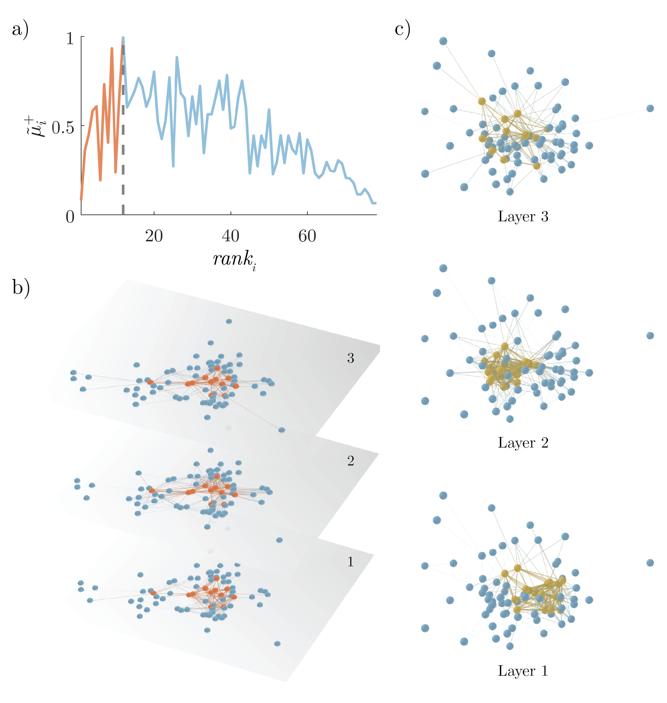
The nodes of the multiplex are ranked according to their richness $\mu$, so that the node $i$ with the best rank, i.e. $rank_{i}=1$, is the node with the largest value of $\mu$, the node ranked 2 is the one with the second largest value of $\mu$, and so on. We then plot for each node $i$ the value of $\mu_{i}^{+}$ as a function of $rank_{i}$. Finally, the maximum of $\mu_{i}^{+}$ is evaluated as a function of the rank. All nodes with rank to the left of such a value are part of the multiplex core, whereas the remaining ones are part of the periphery. As an illustrative example of how our method works in Fig. 1 we report the curve $\mu_{i}^{+}$ as a function of $rank_{i}$ obtained in the case of the Top Noordin Terrorist network, a multiplex network of $N=78$ individuals with three layers (encoding information about mutual trust, common operations and exchanged communication between terrorists), which has been used as a benchmark to test measures and models of multiplex networks battiston14 . Coefficients $c^{[\alpha]}$ were chosen, in this case, to be inversely proportional to $K^{[\alpha]}$ to compensate for the different densities of the three layers. The resulting multiplex rich core integrates information from all the layers and looks different from the rich cores obtained at each of the three layers by a standard single-layer rich core analysis.

II.2 Testing the method on multiplex networks with tunable core similarity

A network with a well defined core-periphery structure has a high density of links among core nodes. With a suitable labeling of the nodes, the adjacency matrix of the network can be decomposed into four different blocks: a dense diagonal block encoding information on core-core links, a sparser diagonal block describing links among peripheral nodes, and two off-diagonal blocks encoding core-periphery edges. The key feature of such block-structure is that $\rho_{1}\gg\rho_{3}$, i.e. the density $\rho_{1}$ of the core-core block is much higher than that of the periphery-periphery block, $\rho_{3}$. As first noted by Borgatti and Everett borgatti00 , the density $\rho_{2}$ of the off-diagonal blocks is typically not a crucial factor to characterise a core-periphery structure.

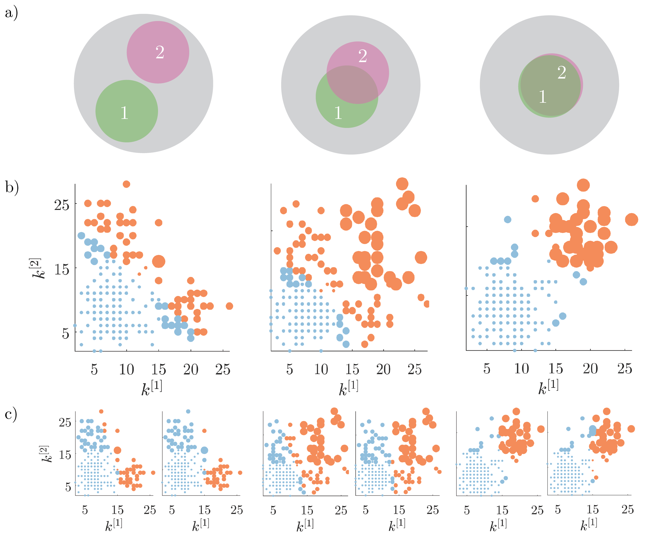
In order to test how our method works on multiplex networks with different structures, we have introduced a model to produce synthetic multiplex networks with tunable core similarity. In particular, we have constructed networks in which, each of the $M=2$ layers has $N=250$ nodes and $N_{c}=50$ of them belong to the core. Each layer has the same average node degree $\langle k\rangle=10$, and the same set of parameters $\rho_{1}>\rho_{2}>\rho_{3}$ to describe its core-periphery structure. Our model allows to control the number of nodes that are both in the core of layer 1 and in the core of layer 2. (see Methods for the choice of the parameters and related discussion).

In order to quantify the similarity among cores at different layers, we introduce the core similarity $S_{c}^{[\alpha]}$ of layer $\alpha$ with respect to the other layers as:

$$S_{c}^{[\alpha]}=\frac{1}{(M-1)}\sum_{\beta\neq\alpha}^{M}\frac{I_{c}^{[\alpha\beta]}}{N_{c}^{[\alpha]}},$$ (3)

where $I_{c}^{[\alpha\beta]}$ is the number of nodes which belong to the core of both layer $\alpha$ and layer $\beta$, whereas $N_{c}^{[\alpha]}$ is the size of the core at layer $\alpha$. The core similarity $S_{c}^{[\alpha]}$ ranges in $[0,1]$. When layer $\alpha$ does not share core nodes with any other layers we have $S_{c}^{[\alpha]}=0$, when all its core nodes also belong to the cores of the other layers $S_{c}^{[\alpha]}=1$, and when on average only half of them are part of the cores on each other level $S_{c}^{[\alpha]}=1/2$. The average core similarity of the multiplex can then be computed as $S_{c}=(1/M)\sum_{\alpha=1}^{M}S_{c}^{[\alpha]}$.

In Fig. 2 we show results for three multiplex networks with different core similarity. In Fig. 2(a) we consider a multiplex with $S_{c}=0$. The cores of the two layers are not overlapping, with many nodes with high degree in one layer having low degree in the other one. In this case, the multiplex core of the system is formed by those nodes with sufficiently high multiplex richness. In Fig. 2(b) we consider a multiplex with $S_{c}=1/2$. Half of the core nodes are shared with the other level of the system, and half are typical of each level. The block representation of the two layers is partially overlapping, and the nodes are spread uniformly over the $(k_{i}^{[2]}$ vs $k_{i}^{[1]}$ plane. The multiplex core of the system in this case is formed by nodes which are part of the core on both layers, but also by nodes scoring extremely high in one layer, despite being periphery in the other one. At last, in Fig. 2(c) we consider a multiplex with $S_{c}=1$. The block structure of the two layers is equivalent, the node degrees $k^{[1]}$ and $k^{[2]}$ at the different levels are correlated and most of the nodes belonging to each core are in the multiplex core of the system.

Figure 2: Core-periphery structure in synthetic multiplex networks with different core similarity. In panel (a) we sketch multiplex networks with $M=2$ layers, $N=250$ nodes and different levels of core similarity, namely $S_{c}=0$ (left column), $S_{c}=1/2$ (central column) and $S_{c}=1$ (right column). In panel (b) the nodes are placed in a two dimensional plane according to their degree at each layer. The size of each dot is proportional to the multiplex richness $\mu_{i}$ of the node, (with $c^{[1]}=1,c^{[2]}=0$). Nodes belonging to the multiplex cores are usually placed in the right-top corner of the plots and are colored orange, while the multiplex periphery is in blue. In panel (c) we report results obtained for two cases with $c^{[1]}\neq c^{[2]}$, namely: $(c^{[1]}=0.75,c^{[2]}=0.25)$ where the core is biased towards the important nodes of the first layer (left), and $(c^{[1]}=1,c^{[2]}=0)$, where the core corresponds to the core of the first layer (right).

II.3 Merging structure and function to extract the connectome’s core

We have applied our method to investigate the human connectome by considering, at the same time, structural and functional information. We have therefore constructed a multiplex human connectome network formed by one structural layer and one functional layer. The two layers were obtained by first averaging brain connectivity matrices estimated respectively from diffusion tensor imaging (DTI) and functional magnetic resonance imaging (fMRI) data in $171$ healthy individuals. Each of the two layers is then thresholded by fixing the average node degree $\langle k\rangle$ (Methods).

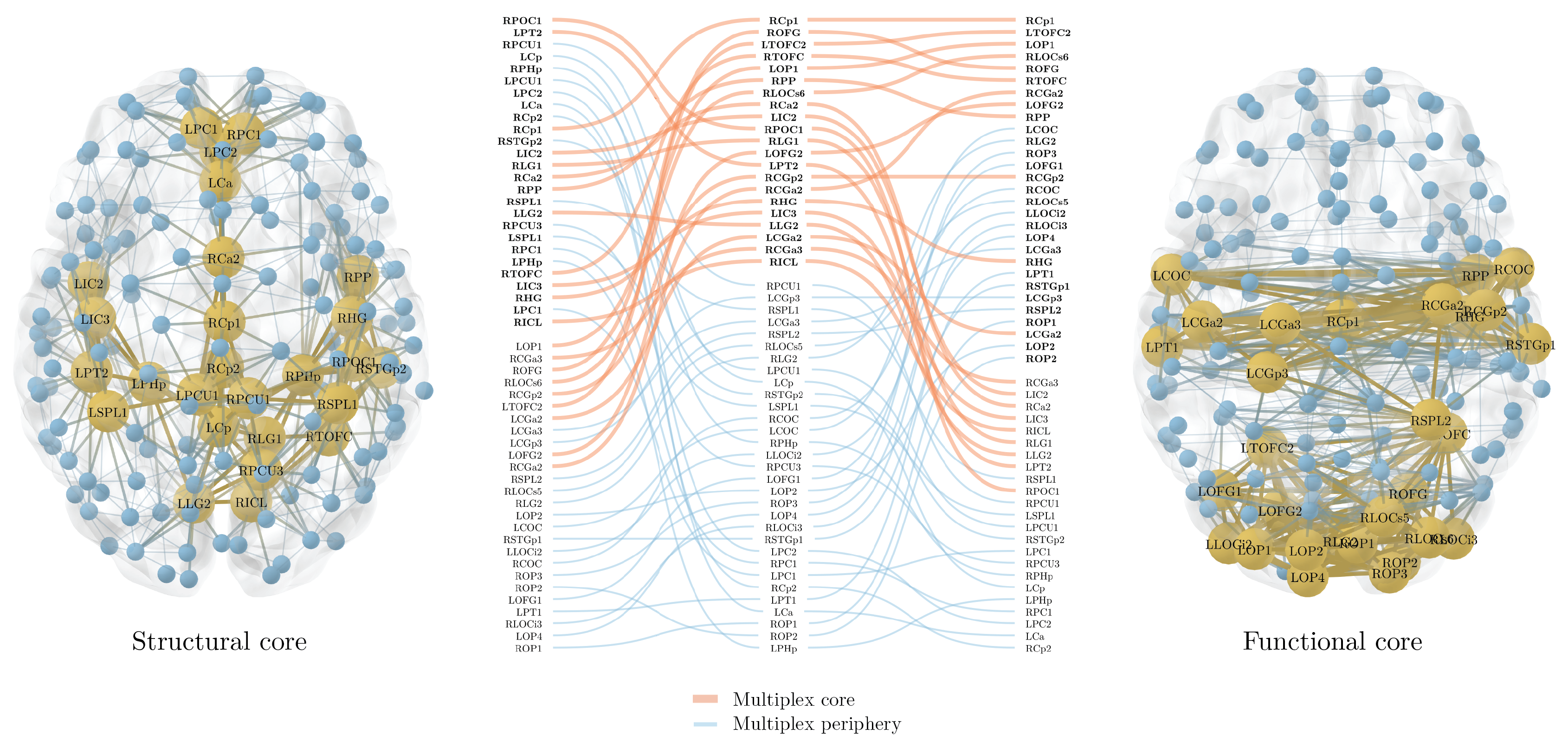
In Fig. 3 we report the two cores found by separately analysing the two layers, together with the multiplex core obtained by our method. The figure refers to the case of a representative threshold corresponding to an average node degree $\langle k\rangle=7$. We notice that the cores of the structural and functional layers are only partially overlapping, with a value of cover similarity of $S_{c}=0.15$. Interestingly, ventral brain areas mainly constitute the structural core, while more dorsal regions appear in the functional core.

Information at the two layers is integrated by our method to extract the multiplex core of the human connectome. Brain regions of interest (ROIs, Table S1) that are in the core of both structural and functional layers also tend to be in the core of the multiplex. Instead, ROIs being in the periphery of both layers tend to be excluded from the multiplex core. However, exceptions may exist depending on the multiplex richness of the nodes. For example, the posterior part of the right precentral gyrus (RCGa3), which is in the periphery of both the structural and functional layer, is eventually assigned to the multiplex core, because of its relatively high rank score in the two layers. The situation appears even less predictable for ROIs that are in the core of one layer and in the periphery of the other layer. Only occasionally these will belong to the multiplex core. This is the case, for example, of the anterior part of right precentral gyrus (RCGa2) which exhibits a relatively low structural richness but high functional richness, i.e. ranked seventh in the functional core.

Figure 3: Extracting the multiplex core of the human brain from structural and functional information. The structural and functional brain networks filtered with an average node degree $\langle k\rangle=7$ are shown respectively on the left and right side. They are represented from above with the frontal lobe pointing upward. The position of the nodes corresponds to the actual location of the brain regions of interests (ROIs, Table S1). Yellow and large nodes represent the brain regions belonging to the core according to the standard single-layer method. Blue and small nodes code for the ROIs in the periphery. Links are yellow and thick if they connect two ROIs in the core, while they are blue and thin if they connect two peripheral nodes. In the central part of the figure, the ROIs are ranked from top to bottom according to their richness in the structural (left column), functional (right column) and multiplex network (central column). In each column, the labels in bold/normal font stand for the ROIs that are in the core/periphery. For the sake of simplicity, only ROIs that are at least in one core (structural, functional or multiplex) are listed in the three columns. Red/blue and thick/thin lines identify ROIs that go into the core/periphery according to the multiplex approach.

II.4 Revealing new core regions of the human brain

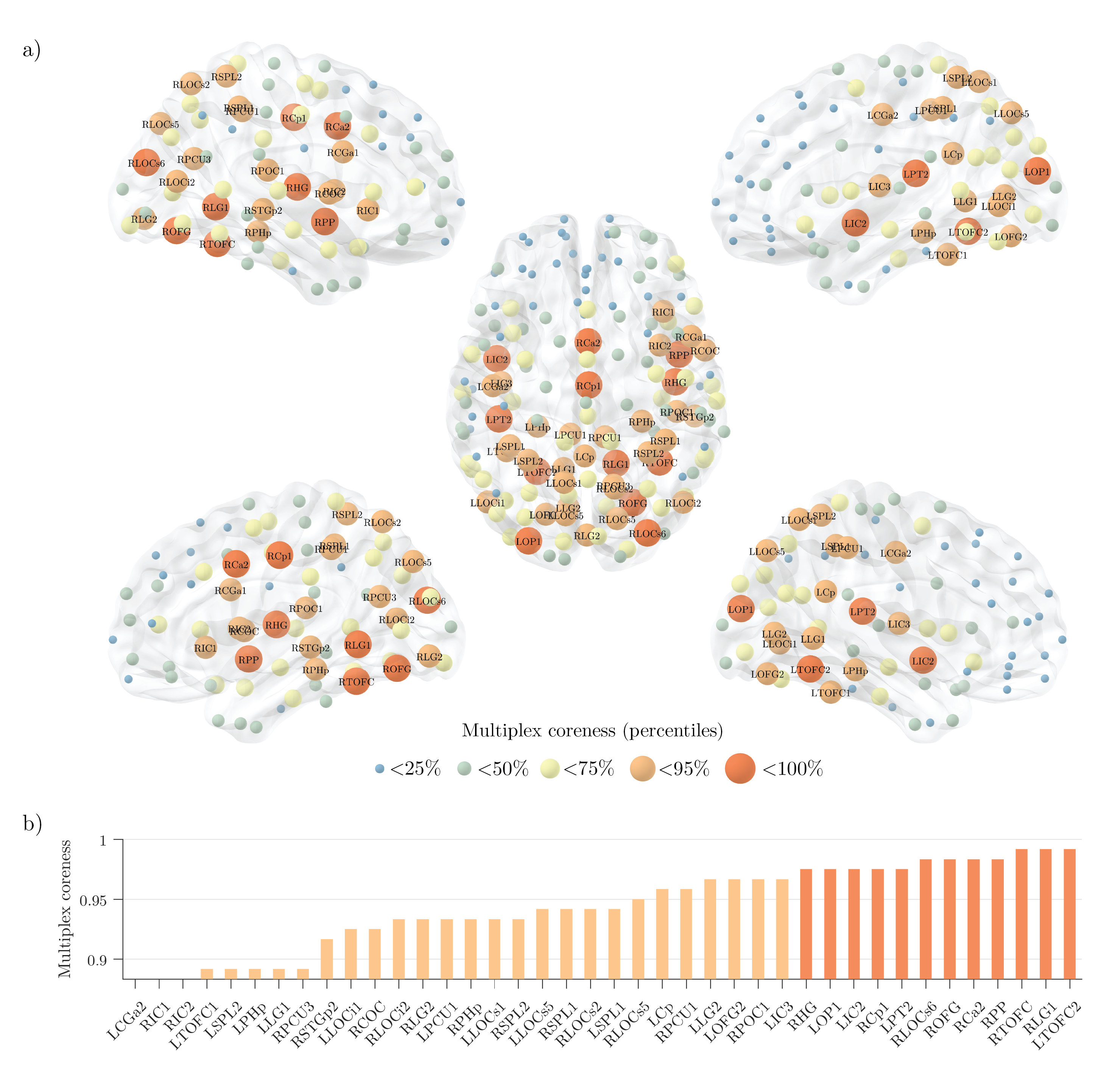
We have extracted the multiplex core-periphery structure of the human brain for the full range of available thresholds $\langle k\rangle=1,2,\ldots,120$ (Methods). In this way, we have been able to calculate the coreness $C_{i}$ of each node $i$, defined as the normalised number of thresholds at which the corresponding ROI is present in the rich core. This allows us to rank ROIs according to their likelihood to be part of the multiplex core and to compare these to the rankings obtained separately for the structural and functional layers. We note that the same approach of investigating the persistence across a set of different filtering thresholds can be applied to any node property. This can turn useful for statistical validation in the case no threshold is universally accepted, as often happens for brain networks.

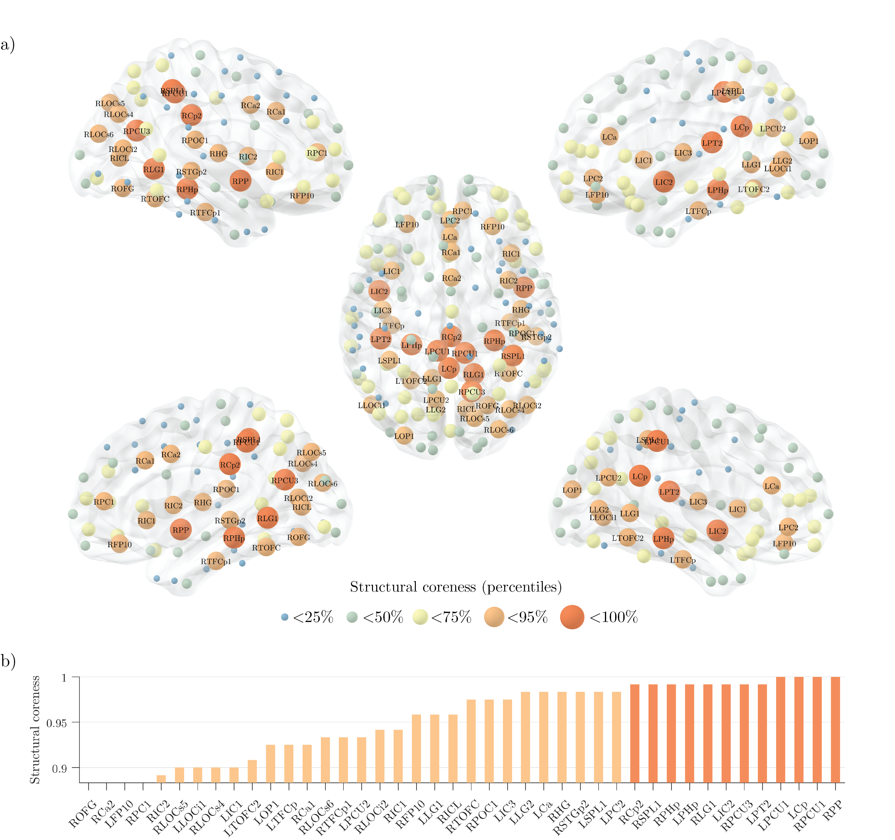
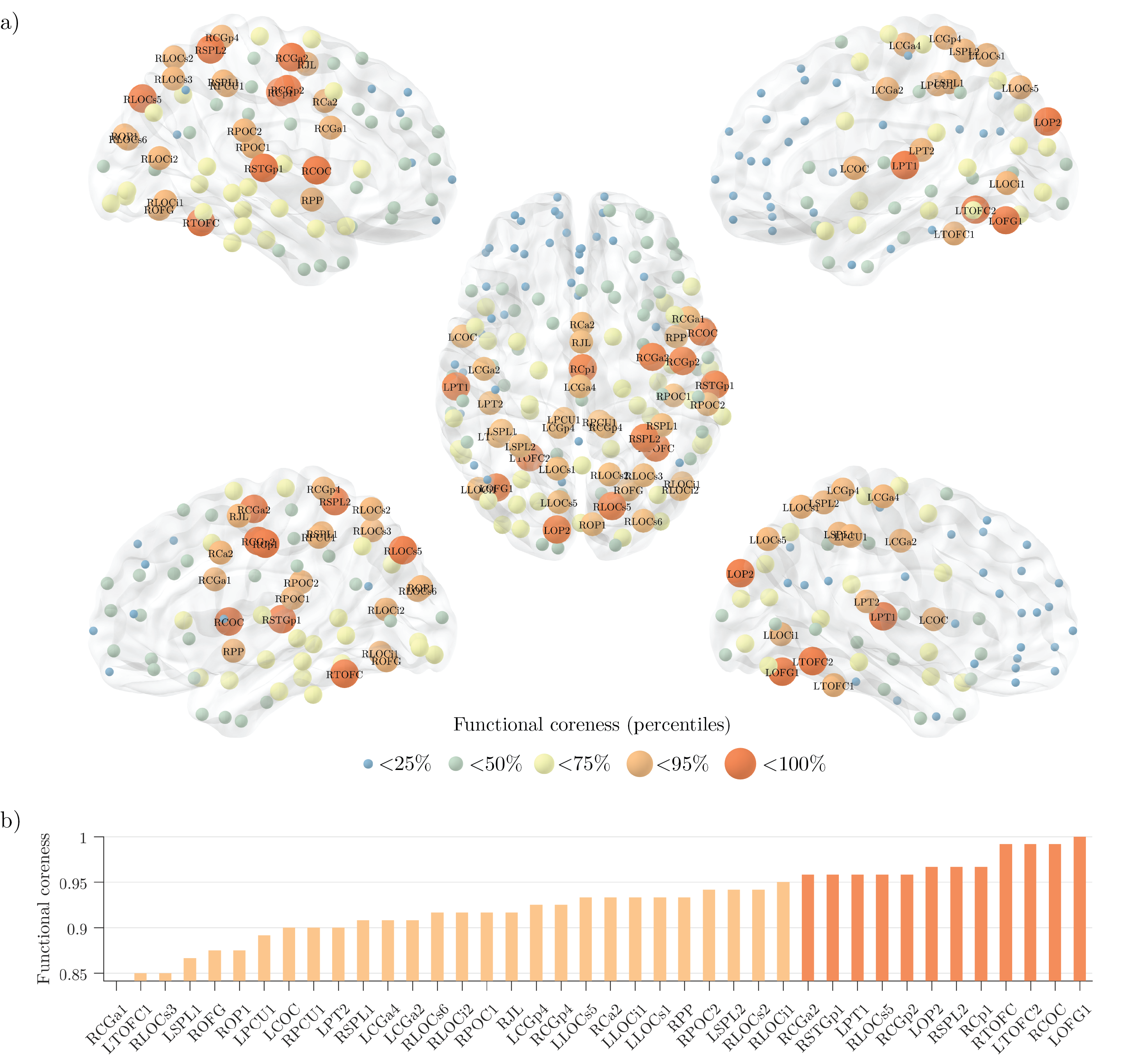
Parietal (pre/cuneus PCU/LOC, superior parietal lobe SPL), cingulate (anterior Ca, posterior Cp), temporal (superior temporal gyrus), insular (insular cortex IC), as well as frontal ROIs (paracingulate PC) mainly constitute the structural core, as shown in Fig. S4. While some overlap exists between the structural and the functional cores, the latter rather tends instead to include occipital (occipital fusiform gyrus OFG, temporo-occipital fusiform cortex TOFC) and central (pre/post central gyrus CGa/CGp) ROIs and, notably, to exclude regions in the frontal lobe (top $25\%$ ROIs, Fig. S5).

Fig. 4 shows the coreness of the multiplex network. As expected, ROIs that are peripheral (i.e., low coreness) in both layers are also peripheral in the multiplex, while ROIs with both a high structural and high functional coreness are typically observed in the multiplex core (e.g., TOFC, OFG, Ca, Cp). Interesting behaviors emerge for those regions typically characterized by high coreness in one layer and low coreness in the other layer. In fact, some of these ROIs are part of the multiplex core, while others are usually found in the multiplex periphery, as shown Fig. 5(a). For regions with different assignment at the two layers, we note that the main contribution to the multiplex richness $\mu_{i}$ comes from the richness at the layer where node $i$ was identified as core. However, not only the average richness at the layer where the node is core is higher than the one at the peripheral layer, but so are fluctuations around the mean. As a consequence, among regions in the structural core but in the functional periphery, those with relatively higher structural richness (degree), such as precuneus PCU, insular cortex IC and posterior cingulate Cp, tend to join the multiplex core no matter the exact value of their functional richness (upper right corner of Fig. 5(a)). Conversely, ROIs with relatively lower structural degree are usually peripheral in the multiplex, and typically located in the pre-frontal cortex PC and frontal lobe FP (lower right corner of Fig. 5(a)), as supported by Fig. 5(b,c). Similarly, for regions in the functional core, those with relatively higher functional degree, such as precentral gyrus CGa and central operculum COC, tend to join the multiplex core (upper left corner of Fig. 5(a)). In contrast, ROIs with relatively lower functional degree, are mostly peripheral in the multiplex, and are located in the parietal operculum POC and superior frontal gyrus SFG (lower left corner of Fig. 5(a)).

Figure 4: The multiplex core of the human connectome. Panel (a) shows the human brain, where regions of interest (ROIs) are highlighted based on their multiplex coreness. The color and size of the nodes are associated to the percentiles of multiplex coreness in each brain region, so that core nodes are larger in size and coloured in red. Left side shows the lateral view of the left hemisphere (top=dorsal, bottom=ventral). Right side shows the lateral view of the right hemisphere (top=dorsal, bottom=ventral). In the middle, the brain is shown from above, with the frontal lobe pointing upward. In panel (b) we report the ROIs corresponding to the $25\%$ highest values of multiplex coreness. The color follows the same legend as in panel (a).

III Discussion

Most networks have a core, a subset of central, tightly interconnected nodes at the heart of the system, which often are the primary responsible for the emergence of collective behaviors. Finding the core-periphery structure of a network is a problem of crucial importance in network science, and a variety of different algorithms have been proposed to define and extract the core in single-layer networks borgatti00 ; csermely13 ; rombach14 ; zhang15 ; barucca16 ; ma15 . However, not all interactions are the same, and networks whose nodes are connected through connections which can vary in meaning and nature, can be better described in terms of networks with many layers kivela14 ; boccaletti14 ; battiston17challenges ; dedomenico13 ; battiston14 . In this work, we introduced a method to identify core-periphery structure in multiplex networks and an algorithmic procedure to extract the multiplex core of the system. The algorithm was first shown to work on synthetic multiplex networks with tunable core similarity, i.e. with controlled overlap between the cores at the different layers. Although the algorithm is very general and can turn useful in several other contexts, it was applied here to a specific problem, namely the identification of the core of the human connectome.

Finding the router regions that ensure integration between the different brain modules and communication in the system as a whole can help answer fundamental questions in neuroscience. The existence of a network core in the brain is considered a prerequisite for neural functioning and cognition, and damages to the core have been recently associated with several neurological or psychiatric diseases van den Heuvel et al. (2013); Gollo et al. (2015); Daianu et al. (2015). Previous studies have addressed the question by mainly considering the structural connectivity of the brain, and by using several techniques, such as $k$-core decomposition, centrality measures, and rich-club analysis Hagmann et al. (2008); Heuvel and Sporns (2011). Standard analyses of the structural connectivity of the human brain agree on the implication of posterior medial and parietal cortical regions in the network core, but are contradictory on the role of frontal regions, such as the mPFC, that are functional components of the default-mode network (DMN) Buckner et al. (2008). Current trends, however, point out that a better understanding of brain networks can only be obtained by considering together the different types of interactions, and this can be achieved by investigating simultaneously both structural and functional brain connectivity battiston17brain ; Crofts et al. (2016); Betzel and Bassett (2017).

Figure 5: Emergent non-trivial core regions in the multiplex brain. Panel (a) shows the scatter plot of the structural, functional and multiplex coreness of the regions of interest (ROIs) in the brain. The color and size of the nodes are associated to the percentile of multiplex coreness across the set of brain regions, as in Fig. 4. Panel (b) reports the average value of multiplex richness $\langle\mu_{i}\rangle$ across the different thresholds for the ROIs with the strongest differences in structural and functional coreness. The color follows the same legend as in panel (a). Panel (c) illustrates the distribution of the ROIs (black points) as a function of their averaged structural and functional degree across all the thresholds. Only the ROIs listed in panel (b) are highlighted according to the same color legend as in panel (a).

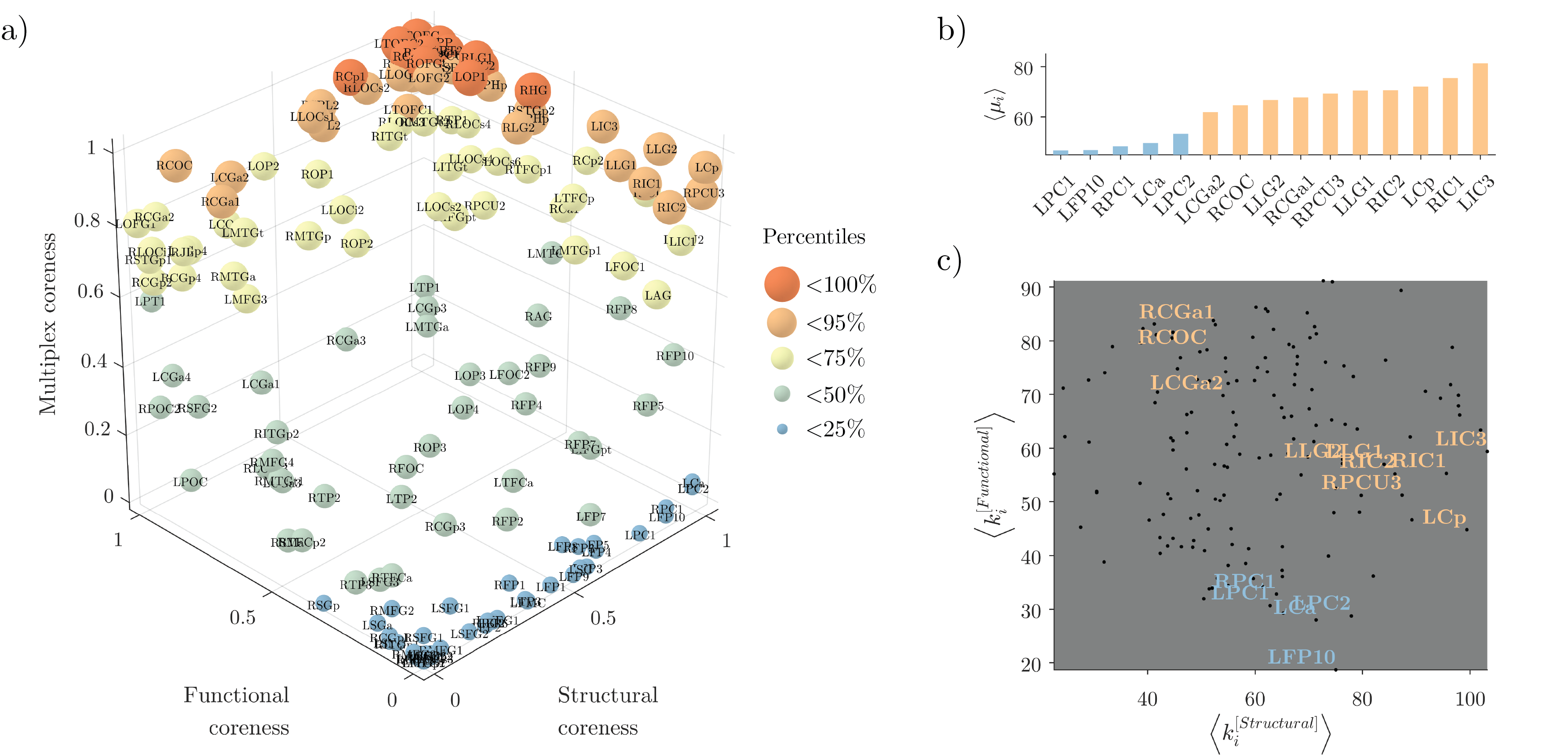
Our method allows to elucidate this aspect, by exploiting also the information available in the functional connectivity, which has surprisingly been poorly explored for such a purpose. The results we have obtained confirm, on the one hand, the systematic involvement of posterior medial (C, IC, PCU) and parietal cortices (e.g., SPL) into the rich core of the human brain. Indeed, these regions have been already identified through the analysis of the structural connectome. On the other hand, the mPFC (e.g., PC and FP), which exhibited a high structural but low functional coreness, is eventually assigned to the periphery (Fig. 5a, lower-right corner). Notably, this result can be predicted by the lower multiplex richness and relatively low structural degree, and not by the solely attitude of frontal areas to be peripheral in the functional brain network (Fig. 5b,c). The exclusion of the mPFC from the rich core supports the hypothesis that default-mode network activity may be mainly driven from highly coupled areas of the posterior medial and parietal cortex, which in turn link to other highly connected regions, such as the medial orbitofrontal cortex Hagmann et al. (2008).

While frontal ROIs are excluded, new regions gain importance and become part of the core because of their higher multiplex richness (see Fig. 5a, upper left corner). Among them, we report areas of the central gyrus (CGa, CGp to a minor extent), which were characterized by a low structural but relatively high functional degree, as shown in Fig. 5(b,c). These regions are part of the primary sensori-motor cortex, which has been shown to be the most extensive of the resting-state components, or networks (out of 8 Heuvel and Pol (2010)), covering $27\%$ percent of the total gray matter in the brain Tomasi and Volkow (2011). The primary sensori-motor component has a high degree of integration (overlap and activity coupling) with all other resting-state networks (e.g., DMN), which is consistent with the increased synchronization of neural activity in cortical regions during sensory processing Srinivasan et al. (1999) and suggests an important role in conscious perception. Notably, ongoing functional connectivity in the primary sensori-motor network, originally revealed by seed-based analysis Biswal et al. (1995); Xiong et al. (1999), has been extensively verified by ICA and clustering methods Salvador et al. (2005); Damoiseaux et al. (2006).

The approach we have proposed here provides an effective tool to integrate mesoscale topological information in brain networks derived from multimodal neuroimaging data. Indeed, multimodal integration in neuroscience is gaining more and more interest due, on the one hand, to the increasing availability of large heterogenous datasets (e.g. HCP http://www.humanconnectomeproject.org, ADNI http://adni.loni.usc.edu) and, on the other hand, to the need of principled ways to define more robust biomarkers. Based on a local fast algorithm, our method allows to extract the core-periphery structure of multiplex brain networks, which can be used to characterize multiscale neural mechanisms (e.g., cross-frequency coupling) and as predictive diagnostics for multifactor brain diseases, such as Alzheimer’s disease.

It is important to notice, that our analysis of the human connectome relies on the assumption that each layer contributes with the same intensity to the definition of the multiplex core. In general, however, the contribution of a layer $\alpha$ can be weighted differently through an opportune choice of the parameter $c^{[\alpha]}$, and this can be used to enhance or reduce the importance of the different types of connectivity. A larger value of $c^{[\alpha]}$ increases the relevance of the corresponding layer until when, in the limit in which $c^{[\alpha]}\to 1$ and the coefficients of all the other layers go to zero, the multiplex core is not any more defined by the topology of all the $M$ layers, but coincides with the core at layer $\alpha$. For instance, setting $c^{[structural]}=1$ and $c^{[functional]}=0$ returns a core based on the anatomical information only, and in agreement with most of the previous literature on such topic (see Fig. S4). As a first attempt to characterize the multiplex core of the human brain, we decided to focus our analysis on the simplest and symmetric case, $c^{[structural]}=c^{[functional]}=1/2$, albeit other combinations are in general possible and can be explored if supported by a plausible rationale. For example, in the case of multifrequency brain networks, one could assign stronger weights to higher frequency layers in order to compensate for $1/f$ frequency scaling of power spectra Bédard et al. (2006).

To conclude, our method to investigate multiplex core-periphery organization in networks shows that the core of the human cortex is made up of known hubs, such as posterior medial and parietal cortical regions, as well as of hubs that were previously overlooked by standard single-layer approaches. Examples are sensori-motor areas. Our findings offer an alternative definition of the rich core of a network, which takes into account not only the anatomical structure but also brain function. We hope our work will trigger additional studies to explore the composition of the multiplex core using functional connectivity acquisition in task-based experiments, in an effort to better integrate the one-to-many relationships that exist between structure and function in the human brain Friston (2011).

IV Methods

IV.1 Multiplex stochastic block model with tunable core similarity

Modelizations of multiplex networks in terms of stochastic block models can be found in Ref. peixoto15 . Here, we introduce a stochastic block model that allows to sample multiplex networks with an assigned value of core similarity $S_{C}$ (see Eq. 3). Suppose we have $N$ nodes and we want to construct a multiplex network having a core-periphery structure at each layer $\alpha=1,\ldots,M$, with $N_{c}^{[\alpha]}$ nodes in the core of layer $\alpha$. In particular, we set $M=2$, $N=250$, $N_{c}^{[1]}=N_{c}^{[2]}=N_{c}=50$, and we create at each layer a core-periphery structure with the same set of densities: $\rho_{1}=0.2$, $\rho_{2}=0.04$ and $\rho_{3}=0.03$. Namely, for each of the two layers, we connect with a probability $\rho_{1}$ two nodes both in the core, with probability $\rho_{2}$ a node in the core and a node in the periphery, and finally with probability $\rho_{3}$ two peripheral nodes. The values of the three parameters were chosen in a way that $\langle k\rangle=10$ on both layers, and the core-periphery structure of each layer is sufficiently strong to be detected with good accuracy, as discussed in the Supplementary Information. Different levels of core similarity are achieved by varying the overlap between core nodes at the two layers. When the two sets of core nodes are completely overlapping, $S_{c}=1$, whereas when the two sets are disjoint $S_{c}=0$. Despite other related formulations of $S_{c}$ are possible, our definition reflects the intuition that when two layers with equal core size share half of the core nodes, then $S_{c}=1/2$.

IV.2 Multiplex richness $\mu_{i}$ and $\mu_{i}^{+}$

The multiplex richness $\mu_{i}$ and $\mu_{i}^{+}$ introduced in Eqs. 1 and 2 are obtained by mean of a simple aggregation of information based on the single layers. In the simplest set-up $c^{[\alpha]}=c=1/M$ for $\alpha=1,\ldots,M$, and the multiplex richness $\mu_{i}$ of a node $i$ is simply proportional to its overlapping degree $o_{i}$ battiston14 . A layer with higher density weighs more in the computation of the multiplex core of a network. In general, coefficients $c^{[\alpha]}$ can be used to modulate the relevance to the layers of the network in order to extract its core. If one wants to have equal contributions to $\mu_{i}$ and $\mu_{i}^{+}$ from all the layers but their number of links $K^{[\alpha]}$ is different - for instance because in some layers it might be easier to establish or measure a connection than in others - a natural choice is to set $c^{[\alpha]}$ to be proportional to $1/K^{[\alpha]}$. In other cases, independently from their density, it might be reasonable to assign different importance to different layers, because of exogenous information. Once again this can be achieved by assigning different values of the coefficients $c^{[\alpha]}$ At last, we notice that Eq. 1 is a particular choice of a more general scenario, where the multiplex richness $\mu_{i}$ is a generic function $f$ of the degree of a node at the different layers:

$$\mu_{i}=f(k_{i}^{[1]},\ldots,k_{i}^{[M]}).$$ (4)

and $\mu_{i}^{+}$ is a function of a generic function $g$:

$$\mu_{i}^{+}=g(k_{i}^{+[1]},\ldots,k_{i}^{+[M]}).$$ (5)

IV.3 Multimodal brain networks

We considered $171$ healthy human subjects from the NKI Rockland dataset http://fcon_1000.projects.nitrc.org/indi/pro/nki.html. We used diffusion weighted magnetic resonance imaging (dwMRI) and functional magnetic resonance imaging (fMRI) to derive respectively structural and functional brain networks in each subject.

We gathered the corresponding connectivity matrices from the USC Multimodal Connectivity Database (http://umcd.humanconnectomeproject.org) (Brown and Van Horn, 2016).

In particular, structural connectivity was obtained using anatomical fiber assignment through the continuous tracking (FACT) algorithm (Mori and van Zijl, 2002). Functional connectivity was computed by means of the Pearson’s correlation coefficient between fMRI signals. More details about the processing steps can be found here (Brown et al., 2012). A total number of $N=188$ regions of interest (ROIs) were available for both structural and functional brain networks, thus resulting in connectivity matrices of size $N\times N$, spatially matched with the MNI152 template (Craddock et al., 2012).

Because we were interested in cortical networks, we removed all subcortical ROIs and obtained connectivity matrices of size $158\times 158$. The full name and acronym for all the ROIs can be found in Table S1. We then averaged the resulting connectivity matrices (after Fisher transformation) across subjects in order to have a population-level representation. At the end, we obtained a structural weighted connectivity matrix $\mathcal{S}$, whose entry $s_{ij}=s_{ji}$ contained the group-average number of axonal fibers between ROIs $i$ and $j$, and a functional weighted connectivity matrix $\mathcal{F}$, whose entry $f_{ij}=f_{ji}$ corresponded to the group-average correlation coefficient between the fMRI signals of ROIs $i$ and $j$.

We used density-based thresholding to derive structural and functional brain networks by removing the lowest values from the connectivity matrices and binarizing the remaining ones De Vico Fallani et al. (2014). We considered a full range of density thresholds, corresponding to an increasing average node degree $\langle k\rangle=1,2,..,120$. The last value was given by the maximal $\langle k\rangle$ observed in the native structural connectivity matrices, which were originally not fully connected. After filtering, for each threshold we combined the resulting structural and functional brain networks into a multiplex network $\mathcal{M}=\{\mathcal{S},\mathcal{F}\}$.

Supplementary information

Stochastic block model for rich cores in single-layer networks

Suppose we have $N$ nodes and we want to construct a single-layer network from which we can identify a partition into two sets: a core of size $N_{c}<N$ and a periphery of size $Np=N-N_{c}$. Here we tested the performance of the single-layer algorithm to detect rich cores ma15 on a simple stochastic block model. Let us consider $N$ nodes from which $N_{c}$ drawn at random are chosen to be part of the network core, whereas the remaining $N_{p}$ are part of the periphery. A network with core-periphery structure is such that its adjacency matrix can be decomposed into four different blocks: a dense diagonal block encoding information on core-core links, a sparser diagonal block describing links among peripheral nodes, and two off-diagonal blocks encoding core-periphery edges. In our block model, we connect two nodes with probability $\rho_{1}$ if they both belong to the core, with probability $\rho_{2}$ if one of them belongs to the core and one to the periphery, and with probability $\rho_{3}$ if they both belong to the periphery, $\rho_{1}\geq\rho_{2}\geq\rho_{3}$. Given a stochastic realisation of the block model, we can extract the rich core of the network and compare it with the groundtruth, i.e. the set of nodes originally labeled as core nodes. In particular, we can test the accuracy of the algorithm for different choice of the parameters $\rho_{1}$, $\rho_{2}$ and $\rho_{3}$.

Given the three probabilities, the expected total number of edges connecting two core nodes is $K_{cc}=\rho_{1}[(N_{c}-1)*N_{c}/2]$, the expected total number of edges connecting two peripheral nodes is $K_{pp}=\rho_{3}[(N-N_{c}-1)*(N-N_{c})/2]$, and the expected total number of edges connecting a node in the core and a node in the periphery $K_{cp}=\rho_{2}[N_{c}*(N-N_{c})]$. The total number of links is $K=K_{cc}+K_{cp}+K_{pp}$.

In the case $\rho_{1}=\rho_{2}=\rho_{3}=\rho$ the nodes are statistically indistinguishable from a structural point of view, the network lacks a core-periphery structure and specifying the value of $\rho$ simply sets the expected average degree of the network $\langle k\rangle=N\rho$. For instance, for $N=250$ and $\rho=0.04$ we obtain $\langle k\rangle=10$ and $K=1250$. Of the different blocks of the adjacency matrix, the exact value of the density of the block encoding links between core and periphery nodes does not play a significant role borgatti00 . For such a reason here we set $\rho_{2}=0.04$, and study the core-periphery structure of the network as a function of $\rho_{1}$, with $\rho_{1}>\rho_{2}$. The higher the value of $\rho_{1}$, the stronger the core-periphery structure of the system. In order to control for the density of the network, as we increases $\rho_{1}$ we have to opportunely decrease the value of $\rho_{3}$. The average degree $\langle k\rangle$ can be kept fixed by setting

$$\rho_{3}=\frac{2}{(Np)*(Np-1)}\biggl{(}K-K_{cc}-K_{cp}\biggr{)}.~{}$$ (6)

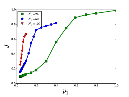
In our case with $N=250$ and $\langle k\rangle=10$, we have $K=1250$ whereas $K_{cc}$ and $K_{cp}$ are set once we fix the core size $N_{c}$ and the value of $\rho_{1}$. In Fig. S1 we show the average Jaccard index $J$ computed for the groundtruth partition and the partition extracted by the algorithm on the stochastic realisations of the network as a function of different values of $\rho_{1}$ for different core size. As shown, $J$ increases quickly until $\rho_{1}=0.2$ and only mildly after this point. This indicates that $\rho_{1}=0.2$, corresponding to a value of $\rho_{3}=0.03$, can be considered as the smallest density of the core-core block at which the core-periphery structure of the network is sufficiently well-defined. For this reason, in the stochastic block model for multiplex networks with different values of core similarity $S_{c}$ described in Fig. 2, where we have $N=250$ and $N_{c}=50$ we set $\rho_{1}=0.2$.

Figure S1: Jaccard index $J$ for the groundtruth core-periphery partition and the partition obtained by the algorithm on realisations of the stochastic block model as a function of $\rho_{1}$ and for different core sizes $N_{c}$.

Given the set of parameters $\rho_{1}$, $\rho_{2}$ and $\rho_{3}$ we can also compute the average degree $\langle k_{c}\rangle$ of core nodes

$$\langle k_{c}\rangle=\rho_{1}(N_{c}-1)+\rho_{2}(N_{p}),$$ (7)

the average degree $\langle k_{p}\rangle$ of the peripheral nodes

$$\langle k_{p}\rangle=\rho_{3}(N_{p}-1)+\rho_{2}(N_{c}).$$ (8)

so that we have

$$\langle k\rangle=\frac{N_{c}\langle k_{c}\rangle+N_{p}\langle k_{p}\rangle}{N}.$$ (9)

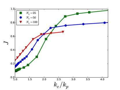
In Fig. S2 we show the average Jaccard index $J$ computed for the groundtruth partition and the partition extracted by the algorithm as a function of $\langle k_{c}\rangle/\langle k_{p}\rangle$.

Figure S2: Jaccard index $J$ for the groundtruth core-periphery partition and the partition obtained by the algorithm on realisations of the stochastic block model as a function of $\langle k_{c}\rangle/\langle k_{p}\rangle$ and for different core sizes $N_{c}$.

Cores of the Top Noordin Terrorists network

In the first Table we report the size $N_{c}$ of the cores of the three layers (mutual trust, common operations, exchanged communications) of the Top Noordin Terrorists network battiston14 and of the multiplex core shown in Fig. 1.

Layer	$N_{c}$
1	17
2	17
3	12
Multiplex	12

In the second Table we report the number of common core nodes $I_{c}$ belonging to the different pairs of layers. The network is characterised by a core similarity $S_{c}=0.38$ ($S_{c}^{[1]}=0.32$, $S_{c}^{[2]}=0.35$, $S_{c}^{[1]}=0.46$. See Eq. 3 in the main text). We also report the number of common core nodes for the multiplex and each layer.

Layer	Layer	$I_{C}$
1	2	6
1	3	5
2	3	6
Multiplex	1	10
Multiplex	2	8
Multiplex	3	7

Core similarity for structural and functional brain networks

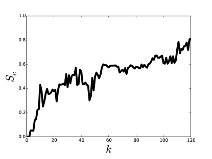
In Fig. S3 we show the core similarity $S_{c}$ for the considered averaged structural and functional networks as a function of different thresholds.

Figure S3: Core similarity $S_{c}$ for the structural and functional networks thresholded at different values of average degree $\langle k\rangle$.

Structural and functional coreness in the human brain

In Figs. S4 and  S5 we report for the ROIs of the human brain the node coreness computed respectively at the structural and functional layer.

Figure S4: Structural core-periphery structure of the human cortex. In panel (a) we show the node structural coreness from different points of view: external view in the top row, internal view in the bottom row. The color and size of each node code for the percentile to which it belongs as specified in the legend. In panel (b) we report the value of structural coreness of the nodes beyond the 75th percentile with the same color code.

Figure S5: Functional core-periphery structure of the human cortex. In panel (a) is represented the functional coreness from different points of view: external view in the top row, internal view in the bottom row. The color and size of each node code for the percentile to which it belongs as specified in the legend. In panel (b) we report the value of functional coreness for the nodes beyond the 75th percentile with the same color code.

List of ROIs

The full list of the considered Regions of Interested (ROIs), and the corresponding abbreviations, can be found in the following Table S1.

Label	Abbreviation	Label	Abbreviation
Left Angular	LAG	Right Central Opercular	RCOC
Left Central Opercular	LCOC	Right Cingulate anterior 1	RCa1
Left Cingulate anterior	LCa	Right Cingulate anterior 2	RCa2
Left Cingulate posterior	LCp	Right Cingulate posterior 1	RCp1
Left Frontal Medial	LFMC	Right Cingulate posterior 2	RCp2
Left Frontal Orbital 1	LFOC1	Right Frontal Orbital	RFOC
Left Frontal Orbital 2	LFOC2	Right Frontal Pole 1	RFP1
Left Frontal Pole 1	LFP1	Right Frontal Pole 10	RFP10
Left Frontal Pole 10	LFP10	Right Frontal Pole 2	RFP2
Left Frontal Pole 2	LFP2	Right Frontal Pole 3	RFP3
Left Frontal Pole 3	LFP3	Right Frontal Pole 4	RFP4
Left Frontal Pole 4	LFP4	Right Frontal Pole 5	RFP5
Left Frontal Pole 5	LFP5	Right Frontal Pole 6	RFP6
Left Frontal Pole 6	LFP6	Right Frontal Pole 7	RFP7
Left Frontal Pole 7	LFP7	Right Frontal Pole 8	RFP8
Left Frontal Pole 8	LFP8	Right Frontal Pole 9	RFP9
Left Frontal Pole 9	LFP9	Right Heschls	RHG
Left Inferior Frontal pars triangularis	LIFGpt	Right Inferior Frontal pars triangularis	RIFGpt
Left Inferior Temporal posterior 1	LITGp1	Right Inferior Temporal posterior 1	RITGp1
Left Inferior Temporal posterior 2	LITGp2	Right Inferior Temporal posterior 2	RITGp2
Left Inferior Temporal temporooccipital	LITGt	Right Inferior Temporal temporooccipital	RITGt
Left Insular 1	LIC1	Right Insular 1	RIC1
Left Insular 2	LIC2	Right Insular 2	RIC2
Left Insular 3	LIC3	Right Intracalcarine	RICL
Left Lateral Occipital inferior 1	LLOCi1	Right Juxtapositional Lobule	RJL
Left Lateral Occipital inferior 2	LLOCi2	Right Lateral Occipital inferior 1	RLOCi1
Left Lateral Occipital superior 1	LLOCs1	Right Lateral Occipital inferior 2	RLOCi2
Left Lateral Occipital superior 2	LLOCs2	Right Lateral Occipital inferior 3	RLOCi3
Left Lateral Occipital superior 3	LLOCs3	Right Lateral Occipital superior 1	RLOCs1
Left Lateral Occipital superior 4	LLOCs4	Right Lateral Occipital superior 2	RLOCs2
Left Lateral Occipital superior 5	LLOCs5	Right Lateral Occipital superior 3	RLOCs3
Left Lateral Occipital superior 6	LLOCs6	Right Lateral Occipital superior 4	RLOCs4
Left Lingual 1	LLG1	Right Lateral Occipital superior 5	RLOCs5
Left Lingual 2	LLG2	Right Lateral Occipital superior 6	RLOCs6
Left Middle Frontal 1	LMFG1	Right Lingual 1	RLG1
Left Middle Frontal 2	LMFG2	Right Lingual 2	RLG2
Left Middle Frontal 3	LMFG3	Right Middle Frontal 1	RMFG1
Left Middle Temporal anterior	LMTGa	Right Middle Frontal 2	RMFG2
Left Middle Temporal posterior 1	LMTGp1	Right Middle Frontal 3	RMFG3
Left Middle Temporal posterior 2	LMTGp2	Right Middle Frontal 4	RMFG4
Left Middle Temporal temporooccipital	LMTGt	Right Middle Temporal anterior	RMTGa
Left Occipital Fusiform 1	LOFG1	Right Middle Temporal posterior	RMTGp
Left Occipital Fusiform 2	LOFG2	Right Middle Temporal temporooccipital 1	RMTGt1
Left Occipital Pole 1	LOP1	Right Middle Temporal temporooccipital 2	RMTGt2
Left Occipital Pole 2	LOP2	Right Occipital Fusiform	ROFG
Left Occipital Pole 3	LOP3	Right Occipital Pole 1	ROP1
Left Occipital Pole 4	LOP4	Right Occipital Pole 2	ROP2
Left Paracingulate 1	LPC1	Right Occipital Pole 3	ROP3
Left Paracingulate 2	LPC2	Right Paracingulate 1	RPC1
Left Parahippocampal posterior	LPHp	Right Paracingulate 2	RPC2
Left Parietal Operculum	LPOC	Right Parahippocampal posterior	RPHp
Left Planum Temporale 1	LPT1	Right Parietal Operculum 1	RPOC1
Left Planum Temporale 2	LPT2	Right Parietal Operculum 2	RPOC2
Left Postcentral 1	LCGp1	Right Planum Polare	RPP
Left Postcentral 2	LCGp2	Right Postcentral 1	RCGp1
Left Postcentral 3	LCGp3	Right Postcentral 2	RCGp2
Left Postcentral 4	LCGp4	Right Postcentral 3	RCGp3
Left Precentral 1	LCGa1	Right Postcentral 4	RCGp4
Left Precentral 2	LCGa2	Right Precentral 1	RCGa1
Left Precentral 3	LCGa3	Right Precentral 2	RCGa2
Left Precentral 4	LCGa4	Right Precentral 3	RCGa3
Left Precuneous 1	LPCU1	Right Precuneous 1	RPCU1
Left Precuneous 2	LPCU2	Right Precuneous 2	RPCU2
Left Subcallosal	LSC	Right Precuneous 3	RPCU3
Left Superior Frontal 1	LSFG1	Right Superior Frontal 1	RSFG1
Left Superior Frontal 2	LSFG2	Right Superior Frontal 2	RSFG2
Left Superior Frontal 3	LSFG3	Right Superior Parietal Lobule 1	RSPL1
Left Superior Parietal Lobule 1	LSPL1	Right Superior Parietal Lobule 2	RSPL2
Left Superior Parietal Lobule 2	LSPL2	Right Superior Temporal posterior 1	RSTGp1
Left Supramarginal anterior	LSGa	Right Superior Temporal posterior 2	RSTGp2
Left Supramarginal posterior	LSMp	Right Supramarginal anterior	RSMa
Left Temporal Fusiform anterior	LTFCa	Right Supramarginal posterior	RSGp
Left Temporal Fusiform posterior	LTFCp	Right Temporal Fusiform anterior	RTFCa
Left Temporal Occipital Fusiform 1	LTOFC1	Right Temporal Fusiform posterior 1	RTFCp1
Left Temporal Occipital Fusiform 2	LTOFC2	Right Temporal Fusiform posterior 2	RTFCp2
Left Temporal Pole 1	LTP1	Right Temporal Occipital Fusiform	RTOFC
Left Temporal Pole 2	LTP2	Right Temporal Pole 1	RTP1
Left Temporal Pole 3	LTP3	Right Temporal Pole 2	RTP2
Right Angular	RAG	Right Temporal Pole 3	RTP3

Table S1: Full list of Regions of Interest (ROIs) and abbreviations. Numbers denote the relative position within a macro area, i.e. higher values stand for more posterior ROIs.

References

- (1)
- (2) R. Albert and A.-L. Barabasi, Rev. Mod. Phys. 74,, 47 (2002).
- (3) M. E. J. Newman, SIAM Review 45, 167-256 (2003).
- (4) S. Boccaletti, V. Latora, Y. Moreno, M. Chavez, D.U. Hwang, Phys. Rep. 424, 175 (2006).
- (5) V. Latora, V. Nicosia, G. Russo, Complex Networks: Principles, Methods and Applications Cambridge University Press (2017)
- (6) R. Milo, S. Shen-Orr, S. Itzkovitz, N. Kashtan, D. Chklovskii, U. Alon Science 298 (5594), 824-827 (2002)
- (7) M. Girvan, M. Newman Proc. Natl. Acad. Sci. USA 99 (12), 7821-7826 (2002)
- (8) S. Fortunato, Phys. Rep. 486, 75 (2010).
- (9) S. P. Borgatti, M. G. Everett. Social Networks, 21, (4) (2000).
- (10) P. Csermely, A. London, L.-Y. Wu, B. Uzzi, Journal of Complex Networks 1, 93-123 (2013)
- (11) M.P. Rombach, M.A. Porter, J.H. Fowler, P.J. Mucha, SIAM Journal on Applied mathematics 74 (1), 167-190 (2014)
- (12) X. Zhang, T. Martin, M.E.J. Newman, Physical Review E 91 (3), 032803 (2015)
- (13) P. Barucca, F. Lillo, Chaos, Solitons & Fractals 88, 244-253 (2016)
- (14) G. Fagiolo, J. A. Reyes, S. Schiavo, Journal of Evolutionary Economics, 20, 4, 479-514, (2009)
- (15) J. P. Boyd, W. J. Fitzgerald, M. C. Mahutga, D. A. Smith, Social Networks, 32 125-137 (2010)
- (16) F. Luo, B. Li, X.F. Wan, R.H. Scheuermann, Bmc Bioinformatics 10 (4), S8 (2009)
- (17) V. Colizza, A. Flammini, M. A. Serrano, and A. Vespignani, Nature Physics 2, 110 (2006).
- (18) S. Zhou and R. J. Mondragon, IEEE Comm. Lett. 8, 180 (2004)
- (19) L.M. Vaquero, M. Cebrian, Scientific reports 3 (2013)
- (20) A. Ma, R.J. Mondragon, PloS one 10 (3) e0119678 (2015)
- Heuvel and Sporns (2011) M. P. v. d. Heuvel and O. Sporns, J. Neurosci. 31, 15775 (2011), ISSN 0270-6474, 1529-2401, URL http://www.jneurosci.org/content/31/44/15775.
- (22) L. Harriger, M.P. Van Den Heuvel, O. Sporns, PloS one 7, e46497 (2012)
- van den Heuvel et al. (2013) M. P. van den Heuvel, O. Sporns, G. Collin, T. Scheewe, R. C. W. Mandl, W. Cahn, J. Goñi, H. E. Hulshoff Pol, and R. S. Kahn, JAMA Psychiatry 70, 783 (2013), ISSN 2168-6238.
- (24) G. Ball et al. “Rich-club organization of the newborn human brain” Proc. Natl. Acad. Sci. USA 111, 7456?7461 (2014)
- (25) M. A. Bertolero, B. T. T. Yeo, and M. D’Esposito Nat. Comm. 8 1277 (2017)
- Bullmore and Sporns (2009) E. Bullmore and O. Sporns, Nature Reviews Neuroscience 10, 186 (2009), ISSN 1471-003X, URL http://www.nature.com/nrn/journal/v10/n3/full/nrn2575.html.
- Stam (2014) C. J. Stam, Nat. Rev. Neurosci. 15, 683 (2014), ISSN 1471-0048.
- (28) S. Boccaletti et al. Physics Reports 544, (1) (2014).
- (29) M. Kivela et al. Journal of Compl. Nets. 2, (3) (2014).
- (30) F. Battiston, V. Nicosia, V. Latora, Eur. Phys. J. Special Topics 226, 401-416 (2017)
- (31) M. De Domenico et al, Phys. Rev. X 3 (4), 041022 (2013)
- (32) F. Battiston, V. Nicosia, V. Latora, Phys. Rev. E 89 (3), 032804 (2014)
- (33) F. Battiston, V. Nicosia, M. Chavez, V. Latora, Chaos 27, 047404 (2017) (2017)
- (34) J. Guillon et al. Scientific Reports 7, 10879 (2017)
- De Domenico et al. (2016) M. De Domenico, S. Sasai, and A. Arenas, Front Neurosci 10, 326 (2016), ISSN 1662-4548.
- (36) P.J. Mucha, T. Richardson, K. Macon, M.A. Porter, J.P. Onnela, Science 328 (5980), 876-878 (2010)
- (37) M. De Domenico, A. Lancichinetti, A. Arenas, M. Rosvall, Phys. Rev. X 5 (1), 011027 (2015)
- (38) F. Battiston, J. Iacovacci, V. Nicosia, G. Bianconi, V. Latora, PloS one 11 (1), e0147451 (2016)
- (39) N. Azimi-Tafreshi, J. Gomez-Gardenes, S.N. Dorogovtsev, Phys. Rev. E 90 (3), 032816 (2014)
- (40) B. Corominas-Murtra, S. Thurner, Interconnected Networks, 165-177 (2016)
- Gollo et al. (2015) L. L. Gollo, A. Zalesky, R. M. Hutchison, M. van den Heuvel, and M. Breakspear, Philos Trans R Soc Lond B Biol Sci 370 (2015), ISSN 0962-8436, URL https://www.ncbi.nlm.nih.gov/pmc/articles/PMC4387508/.
- Daianu et al. (2015) M. Daianu, N. Jahanshad, T. M. Nir, C. R. Jack, M. W. Weiner, M. A. Bernstein, P. M. Thompson, and Alzheimer’s Disease Neuroimaging Initiative, Hum Brain Mapp 36, 3087 (2015), ISSN 1097-0193.
- Hagmann et al. (2008) P. Hagmann, L. Cammoun, X. Gigandet, R. Meuli, C. J. Honey, V. J. Wedeen, and O. Sporns, PLoS Biol 6 (2008), ISSN 1544-9173, URL http://www.ncbi.nlm.nih.gov/pmc/articles/PMC2443193/.
- Buckner et al. (2008) R. L. Buckner, J. R. Andrews-Hanna, and D. L. Schacter, Annals of the New York Academy of Sciences 1124, 1 (2008), ISSN 1749-6632, URL http://onlinelibrary.wiley.com/doi/10.1196/annals.1440.011/abstract.
- Crofts et al. (2016) J. J. Crofts, M. Forrester, and R. D. O’Dea, EPL 116, 18003 (2016), ISSN 0295-5075, URL http://stacks.iop.org/0295-5075/116/i=1/a=18003.
- Betzel and Bassett (2017) R. F. Betzel and D. S. Bassett, NeuroImage 160, 73 (2017), ISSN 1053-8119, URL http://www.sciencedirect.com/science/article/pii/S1053811916306152.
- Heuvel and Pol (2010) M. P. v. d. Heuvel and H. E. H. Pol, European Neuropsychopharmacology 20, 519 (2010), ISSN 0924-977X, 1873-7862, URL http://www.europeanneuropsychopharmacology.com/article/S0924-977X(10)00068-4/fulltext.
- Tomasi and Volkow (2011) D. Tomasi and N. D. Volkow, Cereb Cortex 21, 2003 (2011), ISSN 1047-3211, URL https://academic.oup.com/cercor/article/21/9/2003/377041.
- Srinivasan et al. (1999) R. Srinivasan, D. P. Russell, G. M. Edelman, and G. Tononi, J. Neurosci. 19, 5435 (1999), ISSN 0270-6474, 1529-2401, URL http://www.jneurosci.org/content/19/13/5435.
- Biswal et al. (1995) B. Biswal, F. Zerrin Yetkin, V. M. Haughton, and J. S. Hyde, Magn. Reson. Med. 34, 537 (1995), ISSN 1522-2594, URL http://onlinelibrary.wiley.com/doi/10.1002/mrm.1910340409/abstract.
- Xiong et al. (1999) J. Xiong, L. M. Parsons, J. H. Gao, and P. T. Fox, Hum Brain Mapp 8, 151 (1999), ISSN 1065-9471.
- Salvador et al. (2005) R. Salvador, J. Suckling, M. Coleman, J. Pickard, D. Menon, and E. Bullmore, Cerebral Cortex 15, 1332 (2005).
- Damoiseaux et al. (2006) J. Damoiseaux, S. Rombouts, F. Barkhof, P. Scheltens, C. Stam, S. Smith, and C. Beckmann, Proceedings of the National Academy of Sciences of the United States of America 103, 13848 (2006).
- Bédard et al. (2006) C. Bédard, H. Kröger, and A. Destexhe, Phys. Rev. Lett. 97, 118102 (2006), URL https://link.aps.org/doi/10.1103/PhysRevLett.97.118102.
- Friston (2011) K. J. Friston, Brain Connect 1, 13 (2011), ISSN 2158-0022.
- (56) T.P. Peixoto Phys. Rev. E 92 (4), 042807 (2015)
- Brown and Van Horn (2016) J. A. Brown and J. D. Van Horn, NeuroImage 124, 1238 (2016), ISSN 1053-8119, URL http://www.sciencedirect.com/science/article/pii/S1053811915007624.
- Mori and van Zijl (2002) S. Mori and P. C. M. van Zijl, NMR Biomed. 15, 468 (2002), ISSN 1099-1492, URL http://onlinelibrary.wiley.com/doi/10.1002/nbm.781/abstract.
- Brown et al. (2012) J. A. Brown, J. D. Rudie, A. Bandrowski, V. Horn, J. D, and S. Y. Bookheimer, Front. Neuroinform. 6 (2012), ISSN 1662-5196, URL https://www.frontiersin.org/articles/10.3389/fninf.2012.00028/full.
- Craddock et al. (2012) R. C. Craddock, G. James, P. E. Holtzheimer, X. P. Hu, and H. S. Mayberg, Hum. Brain Mapp. 33, 1914 (2012), ISSN 1097-0193, URL http://onlinelibrary.wiley.com/doi/10.1002/hbm.21333/abstract.
- De Vico Fallani et al. (2014) F. De Vico Fallani, J. Richiardi, M. Chavez, and S. Achard, Phil. Trans. R. Soc. B 369, 20130521 (2014), ISSN 0962-8436, 1471-2970, URL http://rstb.royalsocietypublishing.org/content/369/1653/20130521.