The high energy fate of the minimal Goldstone Higgs

Abstract

We consider a minimal model where the Higgs boson arises as an elementary pseudo-Nambu-Goldstone boson. The model is based on an extended scalar sector with global SO(5)/SO(4) symmetry. To achieve the correct electroweak symmetry breaking pattern, the model is augmented either with an explicit symmetry breaking term or an extra singlet scalar field. We consider separately both of these possibilities. We fit the model with the known particle spectrum at the electroweak scale and extrapolate to high energies using renormalization group. We find that the model can remain stable and perturbative up to the Planck scale provided that the heavy beyond Standard Model scalar states have masses in a narrow interval around 3 TeV.
Preprint: CP³-Origins-2017-050 DNRF90 & HIP-2018/2-TH

I Introduction

The discovery of the Higgs boson at the LHC has verified the Standard Model (SM)-like pattern of electroweak symmetry breaking. A possible interpretation of this discovery is to take the SM particle content (possibly extended by three right handed neutrinos Asaka:2005an ; Asaka:2005pn ) to describe all elementary particle interactions below the Planck energy: with the observed Higgs mass the scalar self coupling does not develop a Landau pole and while the scalar self coupling runs negative around scale $10^{10}$ GeV, this results only in a metastability of the low energy vacuum Degrassi:2012ry ; Antipin:2013sga .

Even so, if the inflationary scale is high enough, one must explain why the Higgs field settled into the false low energy vacuum in spite of large field excursions induced by the inflationary fluctuations EliasMiro:2011aa ; Kobakhidze:2013tn ; Fairbairn:2014zia . In extensions of the SM with larger scalar sectors this problem can be alleviated Gabrielli:2013hma ; Bhattacharya:2014gva , as the presence of additional bosonic degrees of freedom coupling only with the Higgs can overcome the SM contribution of the top quark. However, with a larger scalar sector involving more couplings another problem emerges as one or more of these couplings can develop Landau poles below the Planck scale.

These basic features, following from the renormalization group evolution of the scalar self couplings, are very sensitive to the degrees of freedom and the relative strengths of their couplings within the scalar sector. Therefore, in the absence of direct signal of any new resonance, the vacuum stability and perturbativity of the couplings provide essential theoretical constraints for various BSM scenarios.

An interesting class of SM extensions, where compatibility of the spectrum with the one observed at LHC can be achieved, is the one where the Higgs boson arises as a pseudo-Nambu-Goldstone Boson (pNGB) Schmaltz:2005ky . In this type of models, the Higgs sector can be either elementary or composite. The composite case has been much studied as it allows to address the hierarchy problem. However, it lacks simple dynamics to produce the SM-fermion masses. The elementary case, on the other hand, provides a calculable framework to assess the observed symmetry-breaking pattern and low-energy spectrum  Coleman:1973jx , and facilitates an effective description of flavour physics in terms of Yukawa interactions as in the SM Alanne:2016mmn . Moreover, the vacuum expectation value of the field in the elementary realization does not provide a cutoff for the model. Instead, the model with elementary scalars can be taken as an effective description valid all up to the Planck energy. We will therefore follow the latter route in this paper, and investigate the running of the couplings and the fate of the vacuum in elementary Goldstone Higgs models.

In this paper we consider explicitly the minimal symmetry breaking patterm, $\mathrm{SO}(5)\to\mathrm{SO}(4)$, where the Higgs emerges as a pNGB. It has been showed Alanne:2016mmn that the minimal particle content of $\mathrm{SO}(5)\to\mathrm{SO}(4)$ needs to be extended in order to have a non-trivial vacuum. There are two basic extensions: One is by adding an explicit breaking term which couples to the singlet and the other is by adding a new scalar which couples to the $\mathrm{SO}(5)\to\mathrm{SO}(4)$ scalar multiplet. We will separately consider these two possibilities.

The paper is organised as follows: In section II we review briefly the $\mathrm{SO}(5)\to\mathrm{SO}(4)$ model where the Higgs is an elementary pseudo Goldstone Boson and determine the $\beta$-functions. In section III we examine the running of the couplings in the case with an explicit breaking term. In section IV we examine the running of the couplings in the case with an extra scalar and in section V we present our conclusions.

II The Minimal Model

The minimal extension of SM leading to pNGB Higgs can be written as a linear $\sigma$-model over the coset SO(5)/SO(4). The general SO(5) invariant potential in terms of SO(5) vector $\Sigma$ is

$$V_{0}=\frac{m^{2}}{2}\Sigma^{\dagger}\Sigma+\frac{\lambda}{4!}(\Sigma^{\dagger}\Sigma)^{2}.$$ (1)

The electroweak gauge group is identified within the SU(2)${}_{L}\times$SU(2)_R subgroup of SO(4). Then the vacuum of the theory can be parametrized as a superposition between a vacuum which preserves the electroweak symmetry, $E_{0}=(0,0,0,1,0)^{T}$, and a vacuum which breaks the electroweak symmetry, $E_{B}=(0,1,0,0,0)^{T}$, as

$$E_{\theta}=\cos\theta\,E_{0}+\sin\theta\,E_{B},$$ (2)

The $\mathrm{SO}(5)$ scalar multiplet can then be written as

$$\Sigma=\left(\sigma+i\pi_{a}X_{\theta}^{a}\right)E_{\theta},$$ (3)

where $X_{\theta}^{a}$ are the broken generators of the $\mathrm{SO}(5)\to\mathrm{SO}(4)$ and can be found in appendix A, $\pi_{a}$ are the Goldtone Bosons and $\sigma$ is a masive scalar field and the only field which obtains a nonzero vacuum expectation value (vev).

The scalar multiplet can be parametrized in many ways. For our purposes, it is most convenient to rewrite it in the basis of eigenstates under the electroweak interactions, i.e. a complex doublet with a neutral and a charged component and a real scalar singlet. In terms of the $\sigma$ field and the Goldstone Bosons, the doublet and the singlet are:

$$H=\frac{1}{\sqrt{2}}\begin{pmatrix}\pi_{1}+i\pi_{2}\\ \sigma\sin\theta+\pi_{4}\cos\theta+i\pi_{3}\end{pmatrix}\qquad\text{and}\qquad S=\sigma\cos\theta-\pi_{4}\sin\theta.$$ (4)

In this basis the higher order potential is

$$V=m_{h}^{2}H^{\dagger}H+m_{s}^{2}S^{2}+\lambda_{1}\left(H^{\dagger}H\right)^{2}+\lambda_{2}S^{4}+\lambda_{3}H^{\dagger}HS^{2}.$$ (5)

The three couplings introduced in Eq. (5) and represented in figure 1 are derived, at tree level, from the single coupling $\lambda$ appearing in Eq. (1). However, they will run differently due to different higher order contributions to each coupling $\lambda_{1}$, $\lambda_{2}$ and $\lambda_{3}$.

The stability constraints on the scalar couplings are

$$\lambda_{1}\geq 0,\qquad\lambda_{2}\geq 0,\qquad\lambda_{3}+2\sqrt{\lambda_{1}\lambda_{2}}\geq 0.$$ (6)

where $\lambda_{1}$ and $\lambda_{2}$ are strictly positive, but $\lambda_{3}$ is allowed to take negative values within the bound implied by the above equation.

Figure 1: shows the three different three-level Feynman diagrams for the $\mathrm{SO}(5)\to\mathrm{SO}(4)$ theory.

The gauge interactions are determined, as in Alanne:2014kea ; Gertov:2015xma , from the kinetic term:

$$\mathcal{L}_{\text{kin}}=\left(D_{\mu}\Sigma\right)^{\dagger}D^{\mu}\Sigma,$$ (7)

where the covariant derivative is

$$D_{\mu}=\partial_{\mu}\Sigma-ig_{w}W^{a}T^{a}_{L}\Sigma+ig_{y}BT^{3}_{R}\Sigma.$$ (8)

The $T_{L}$ and $T_{R}$ are the generators of the $\mathrm{SU}_{L}(2)$ and $\mathrm{SU}_{R}(2)$ respectively and they are explicitly defined in Appendix A.

The Lagrangian for the Yukawa couplings is

$$\mathcal{L}_{\text{Yuk}}^{\text{top}}=y_{t}(Qt^{c})^{\dagger}_{\alpha}P_{\alpha}\Sigma,$$ (9)

where $\alpha$ is a $\mathrm{SU}_{L}(2)$ index and $P_{\alpha}$ are pseudo-projectors defined as

$$P_{1}=\frac{1}{\sqrt{2}}\big{(}0,\,\,0,\,\,1,\,\,i,\,\,0\big{)}\qquad\text{and}\qquad P_{2}=\frac{1}{\sqrt{2}}\big{(}1,\,\,i,\,\,0,\,\,0,\,\,0\big{)}\,.$$ (10)

These pseudo-projectors pick the correct parts of the doublets in $\Sigma$. We will consider here only the Yukawa interactions of the top quark as these are the ones giving the dominant contribution from fermions to the beta functions.

The beta functions describing the running of the couplings above the renormalization scale $\mu_{0}$ are computed using the standard methods Machacek:1983fi ; Machacek:1983tz ; Machacek:1984zw . The beta functions at one-loop order for the three scalar couplings in this theory are

$$\begin{split}\beta_{\lambda_{1}}&=\frac{1}{(4\pi)^{2}}\left(\frac{9}{8}g_{w}^{4}+\frac{3}{4}g_{w}^{2}g_{y}^{2}+\frac{3}{8}g_{y}^{4}-9g_{w}^{2}\lambda_{1}-3g_{y}^{2}\lambda_{1}-6y_{t}^{4}+12\lambda_{1}y_{t}^{2}+24\lambda_{1}^{2}+2\lambda_{3}^{2}\right)\\ \beta_{\lambda_{2}}&=\frac{1}{(4\pi)^{2}}\left(72\lambda_{2}^{2}+2\lambda_{3}^{2}\right)\\ \beta_{\lambda_{3}}&=\frac{1}{(4\pi)^{2}}\left(-\frac{9}{2}g_{w}^{2}\lambda_{3}-\frac{3}{2}g_{y}^{2}\lambda_{3}+6y_{t}^{2}\lambda_{3}+12\lambda_{1}\lambda_{3}+24\lambda_{2}\lambda_{3}+8\lambda_{3}^{2}\right).\end{split}$$ (11)

However, there is an important caveat that we need to take into account now. In Alanne:2016mmn some of the authors of the present paper found that the gauge and Yukawa interactions are not enough to align the vacuum away from zero in any $\mathrm{SO}(N)\to\mathrm{SO}(N-1)$ theory where the Higgs is an elementary pNGB. Two ways of solving this issue were put forward in Alanne:2016mmn : First, by adding a small explicit breaking term competing with the one loop potential contribution, and second, by adding an extra scalar field which couples to $\Sigma$ via a portal coupling. Within the second approach three new couplings need to be introduced.

In the following two section we will answer the relevant question of what is the behaviour of the running of all the couplings in both scenarios at high energy. To our knowledge these is the first comprehensive analysis of these theories at short distances.

III $\mathrm{SO}(5)\to\mathrm{SO}(4)$ + explicit breaking term

In this section we consider the tree level potential given in eq. (1). At some renormalization scale, $\mu_{0}$, the three scalar couplings are assumed to combine so that the potential is SO(5) invariant. Furthermore, assuming perturbative values of the couplings, the one-loop corrections are computable using the Coleman-Weinberg potential which is defined as

$$\delta V(\Phi)=\frac{1}{64\pi^{2}}\text{Str}\left[\mathcal{M}_{0}^{4}(\Phi)\left(\log\frac{\mathcal{M}_{0}^{2}(\Phi)}{\mu_{0}^{2}}-C\right)\right]+V_{GB}\,,$$ (12)

where $\mathcal{M}_{0}$ is the mass matrix, Str is the supertrace where the sums over scalar, fermion and vector degrees of freedom are weighted with factors $1$, $-2$ and $3$, respectivley. The constant $C$ depends on the particle type and is $C=3/2$ for scalars and fermions and $C=5/6$ for gauge bosons. The factor $V_{GB}$ represents the one-loop corrections from the Goldstone bosons which we will neglect since their contributions to the potential are much smaller than the correction from massive particles.

As argued above we can ensure existence of a nontrivial vacuum by adding an explicit symmetry breaking term, given by

$$V_{B}=C_{B}v^{3}S\,.$$ (13)

On the basis of the results in Alanne:2016mmn we take $C_{B}>0$ and small, in order to have a small breaking. Concretely, we consider $0<C_{B}<0.1$. Imposing the correct mass of the Higgs and minimizing of the potential wrt. $\theta$ give us an upper and lower bound on the mass $M_{\sigma}$ which is $1.35\,\text{TeV}<M_{\sigma}<3.20\,\text{TeV}$. This corresponds to a coupling $\lambda$ in the interval $0.29<\lambda<1.68$. These are the values below the renormalization scale $\mu_{0}$, where we can describe the theory through the Coleman-Weinberg potential. The renormalization scale $\mu_{0}$ is a function of $M_{\sigma}$ and in the allowed interval of $M_{\sigma}$ it is nearly constant with the value $\mu_{0}\approx 2\,\text{TeV}$.

Above the renormalization scale the coupling $\lambda$ splits into three couplings which run according to their respective beta functions. At the renormalization scale the value of all three couplings is determined by $\lambda$. The couplings $\lambda_{1}$ and $\lambda_{2}$ must be positive and we require that all couplings remain free of Landau poles all the way to the Planck scale. From these constraints we find $0.50<\lambda<0.90$ which corresponds to a sigma mass in the interval $2.93\,\text{TeV}<M_{\sigma}<3.10\,\text{TeV}$ and $\sin\theta$ in the interval $0.034<\sin\theta<0.043$. Finally the vacuum is found to be between $5.66\,\text{TeV}<v<7.18\,\text{TeV}$. These constraints are illustrated in figure 2. The figure show the scale evolution of the couplings $\lambda_{1}$ (red), $\lambda_{2}$ (orange) and $\lambda_{3}$ (blue), and the constraints restrict the running of the couplings to lie between the corresponding solid and dashed curves.

Figure 2: The figure shows the running of the couplings above 2 TeV, where the dashed lines correspond to the lower bound on the combined $\lambda$ and the solid lines correspond to the upper bound. The red lines are $\lambda_{1}$, the blue lines are $\lambda_{2}$ and the orange lines are $\lambda_{3}$. The initial values of the three running couplings all depend on the same coupling $\lambda$. On the plot $\lambda_{2}$ does however start in a value different from the two other couplings, this is because of the different normalizations.

The relationship between $\lambda$ and $M_{\sigma}$ below $\mu_{0}=2\,\text{TeV}$ (i.e. where the coupling does not run) is plotted in the left panel of figure 3.

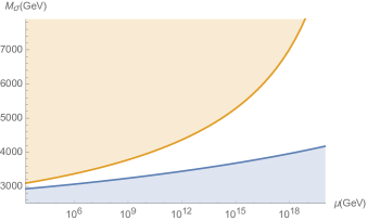
Figure 3: Left panel: The blue line shows the relationship between $\lambda$ and $M_{\sigma}$ below $\mu_{0}=2\,\text{TeV}$ when the correct Higgs mass is imposed. The green area is excluded due to Landau poles and the orange area is excluded due to stability. This gives a narrow window for $M_{\sigma}\in[2.93,3.10]\,\text{TeV}$ indicated by the grey vertical lines. Right panel: Running of $M_{\sigma}$. The shaded blue area is excluded due to stability and the orange area due to Landau poles. The true running of $M_{\sigma}$ lies on a curve in the white region and depends on the value of $\lambda$ at $\mu_{0}=1.70\,\text{TeV}$.

The blue line shows the relation between $M_{\sigma}$ and $\lambda$ when the potential is minimised with respect to $\sin\theta$ and the correct mass of the Higgs is imposed. The shaded regions are excluded due to perturbativity and stability constraints on $\lambda$ and the grey vertical lines correspond to $M_{\sigma}=2.93\,\text{TeV}$ and $M_{\sigma}=3.10\,\text{TeV}$ respectively. The right panel of figure 3 shows the mass of the $\sigma$ particle, $M_{\sigma}$, as function of the renormalization scale $\mu$. The blue shaded region is excluded due to vacuum stability as the couplings run. The orange shaded region is excluded due to the perturbativity of the couplings (i.e. the absence of Landau poles below the Planck scale). This means that the running of $M_{\sigma}$ lies on a curve in the white region.

As in the Elementary Goldstone Higgs model, first proposed in Alanne:2014kea ; Gertov:2015xma , the observed Higgs boson is a superposition between the $\sigma$ and the $\pi_{4}$ particles. This superposition can be described by a mixing angle $\alpha$. For small values of $\theta$ this can be approximated as

$$\begin{split}\alpha\approx&\frac{\pi}{2}-\frac{6\theta^{3}v^{4}}{54M_{\sigma}^{8}+192\pi^{2}M_{\sigma}^{6}v^{2}-11C_{B}M_{\sigma}^{4}v^{4}}\\ &\qquad\quad\left[6BM_{\sigma}^{4}-A\left(C_{B}v^{4}-13M_{\sigma}^{4}+6M_{\sigma}^{4}\log\frac{M_{\sigma}^{2}}{\theta^{2}v^{2}}\right)\right]+\mathcal{O}(\theta^{5}),\end{split}$$ (14)

where A and B are coefficients depending only on gauge and Yukawa couplings. They are given by

$$\begin{split}A=&3\left(\frac{g_{w}^{4}}{8}+\frac{1}{16}\left(g_{w}^{2}+g_{y}^{2}\right)^{2}\right)-3y_{t}^{4},\\ B=&\frac{3}{16}\left[\left(g_{w}^{2}+g_{y}^{2}\right)^{2}\left(\log\frac{g_{w}^{2}+g_{y}^{2}}{4}-\frac{5}{6}\right)+2g_{w}^{4}\left(\log\frac{g_{w}^{2}}{4}-\frac{5}{6}\right)\right]-3y_{t}^{4}\left(2\log\frac{y_{t}^{2}}{2}-3\right).\end{split}$$ (15)

If $\alpha$ is close to $\frac{\pi}{2}$ the observed Higgs is mostly the Goldstone Boson, $\pi_{4}$, while the observed Higgs is mostly the scalar $\sigma$ if $\alpha$ is close to zero. In the interval for $M_{\sigma}$ found above, $\alpha$ is very close to $\frac{\pi}{2}$ and the observed Higgs is almost the Goldstone boson. Defining the two mass eigenstates $h_{1}=\cos\alpha\,\sigma+\sin\alpha\,\pi_{4}$ and $h_{2}=-\sin\alpha\,\sigma+\cos\alpha\,\pi_{4}$, where $h_{1}$ is the observed Higgs, we can calculate the self couplings of the physical mass eigenstates:

$$\begin{split}\lambda_{h_{1}h_{1}h_{1}}=\frac{3M_{\sigma}^{2}\cos\alpha}{v},\qquad\lambda_{h_{1}h_{1}h_{2}}=\frac{M_{\sigma}^{2}\sin\alpha}{v},\qquad\lambda_{h_{1}h_{2}h_{2}}=\frac{M_{\sigma}^{2}\cos\alpha}{v},\\ \lambda_{h_{2}h_{2}h_{2}}=\frac{3M_{\sigma}^{2}\sin\alpha}{v},\qquad\lambda_{h_{1}h_{1}h_{1}h_{1}}=\frac{3M_{\sigma}^{2}}{v^{2}},\qquad\lambda_{h_{1}h_{1}h_{1}h_{2}}=0,\\ \lambda_{h_{1}h_{1}h_{2}h_{2}}=\frac{M_{\sigma}^{2}}{v^{2}},\qquad\lambda_{h_{1}h_{2}h_{2}h_{2}}=0,\qquad\lambda_{h_{2}h_{2}h_{2}h_{2}}=\frac{3M_{\sigma}^{2}}{v^{2}}.\end{split}$$ (16)

Note that the quartic couplings do not depend on the mixing angle $\alpha$ and the quartic couplings for $h_{1}$ and $h_{2}$ are identical. However, the trilinear couplings do depend on $\alpha$. When $\alpha$ is close to $\frac{\pi}{2}$ the trilinear self coupling of $h_{1}$ is very small while the trilinear self coupling of $h_{2}$ is large. In the interval on the mass $M_{\sigma}$ found above, we can calculate the ratio of the two trilinear couplings with the trilinear coupling of the SM:

$$1.02\cdot 10^{-3}<\frac{\lambda_{h_{1}h_{1}h_{1}}}{\lambda_{hhh}^{SM}}<2.33\cdot 10^{-3}\qquad\text{and}\qquad 23.5>\frac{\lambda_{h_{2}h_{2}h_{2}}}{\lambda_{hhh}^{SM}}>20.9.$$ (17)

The trilinear coupling for $\lambda_{h_{1}h_{1}h_{1}}$ is very small compared to the corresponding coupling in SM and it is smallest when the $M_{\sigma}$ is smallest. However the behavior of $\lambda_{h_{2}h_{2}h_{2}}$ is the opposite: $\lambda_{h_{2}h_{2}h_{2}}$ is larger than the SM one and it is largest when $M_{\sigma}$ is smallest.

We have therefore shown that this scenario leads to a viable elementary Goldstone Higgs framework valid up to the Planck scale.

IV $\mathrm{SO}(5)\to\mathrm{SO}(4)$ + an extra scalar $\Omega$

Now we turn to the other possibility, namely adding an extra scalar $\Omega$ which couples to $\Sigma$ via a portal coupling. We assume that $\Omega$ is both real and has a $Z_{2}$ symmetry. The new tree level potential is then

$$V_{0}=\frac{m^{2}}{2}\Sigma^{\dagger}\Sigma+\frac{m_{\Omega}^{2}}{2}\Omega^{2}+\frac{\lambda}{4!}\left(\Sigma^{\dagger}\Sigma\right)^{2}+\frac{\tilde{\lambda}}{4}\Sigma^{\dagger}\Sigma\Omega^{2}+\frac{\tilde{\lambda}_{\Omega}}{4!}\Omega^{4}.$$ (18)

As in the previous section, we write the potential in terms of the doublet and singlet fields:

$$V=m_{h}^{2}H^{\dagger}H+m_{s}^{2}S^{2}+m_{\Omega}^{2}\Omega^{2}+\lambda_{1}\left(H^{\dagger}H\right)^{2}+\lambda_{2}S^{4}+\lambda_{3}H^{\dagger}HS^{2}+\lambda_{4}H^{\dagger}H\Omega^{2}+\lambda_{5}S^{2}\Omega^{2}+\lambda_{\Omega}\Omega^{4}\,.$$ (19)

Here the couplings $\lambda_{1}$, $\lambda_{2}$ and $\lambda_{3}$ are, at tree level, determined by the self-interaction $\lambda$ in the SO(5) invariant potential, Eq. (18), and similarly $\lambda_{4}$ and $\lambda_{5}$ are determined by $\tilde{\lambda}$. However, similarly to the situtation treated in the previous section, all these couplings will receive different contributions at one-loop order and, consequently, their running will be different. The beta functions for the six different couplings are:

$$\begin{split}\beta_{\lambda_{1}}&=\frac{1}{(4\pi)^{2}}\left(\frac{9}{8}g_{w}^{4}+\frac{3}{4}g_{w}^{2}g_{y}^{2}+\frac{3}{8}g_{y}^{4}-9g_{w}^{2}\lambda_{1}-3g_{y}^{2}\lambda_{1}-6y_{t}^{4}+12\lambda_{1}y_{t}^{2}+24\lambda_{1}^{2}+2\lambda_{3}^{2}+2\lambda_{4}^{2}\right),\\ \beta_{\lambda_{2}}&=\frac{1}{(4\pi)^{2}}\left(72\lambda_{2}^{2}+2\lambda_{3}^{2}+2\lambda_{5}^{2}\right),\\ \beta_{\lambda_{3}}&=\frac{1}{(4\pi)^{2}}\left(-\frac{9}{2}g_{w}^{2}\lambda_{3}-\frac{3}{2}g_{y}^{2}\lambda_{3}+6y_{t}^{2}\lambda_{3}+12\lambda_{1}\lambda_{3}+24\lambda_{2}\lambda_{3}+8\lambda_{3}^{2}+4\lambda_{4}\lambda_{5}\right),\\ \beta_{\lambda_{4}}&=\frac{1}{(4\pi)^{2}}\left(-\frac{9}{2}g_{w}^{2}\lambda_{4}-\frac{3}{2}g_{y}^{2}\lambda_{4}+6y_{t}^{2}\lambda_{4}+12\lambda_{1}\lambda_{4}+8\lambda_{4}^{2}+4\lambda_{3}\lambda_{5}+24\lambda_{4}\lambda_{\Omega}\right),\\ \beta_{\lambda_{5}}&=\frac{1}{(4\pi)^{2}}\left(4\lambda_{3}\lambda_{4}+24\lambda_{2}\lambda_{5}+16\lambda_{5}^{2}+24\lambda_{5}\lambda_{\Omega}\right),\\ \beta_{\lambda_{\Omega}}&=\frac{1}{(4\pi)^{2}}\left(2\lambda_{4}^{2}+2\lambda_{5}^{2}+72\lambda_{\Omega}^{2}\right).\end{split}$$ (20)

Note the similarity between the beta functions of $\lambda_{3}$ and $\lambda_{4}$, which are the couplings between the scalar doublet and the two scalar singlets. Also note the similarity between the beta functions of $\lambda_{2}$ and $\lambda_{\Omega}$, which are the self-couplings of the two singlets: The new scalar singlet $\Omega$ has interactions which are analogous to the original singlet component $S$ of the SO(5) mutiplet $\Sigma$.

For simplicity we consider the case, where the mass of the new particle $\Omega$ is the same as the mass of $\sigma$. Just as in the previous case, below the renormalization scale $\mu_{0}$ the couplings combine and the $\mathrm{SO}(5)\to\mathrm{SO}(4)$ symmetry is intact. Since the couplings are perturbative, we can use the Coleman-Weinberg potential introduced in (12). However, in this case the mixing $\alpha$ is simpler and given by

$$\alpha\approx\frac{\pi}{2}-\frac{v^{4}\theta^{3}}{9M_{\sigma}^{4}+32\pi M_{\sigma}^{2}v^{2}+\tilde{\lambda}v^{4}}\left[6B-A\left(6\log\frac{M_{\sigma}^{2}}{v^{2}\theta^{2}}-13\right)\right]+\mathcal{O}(\theta^{5})$$ (21)

where $A$ and $B$ are given in (15).

As in the case treated in the previous section, we will now constrain the model by requiring that correct spectrum of physical states is reproduced at low energies, and that the vacuum remains stable at high energies. We also require that the one loop running of the dimensionless couplings is free of Landau poles below the Planck scale. We treat separately the constraints relevant below and above the renormalization scale.

First, below the renormalization scale, we impose the correct mass of the Higgs and demand that the potential is minimized with respect to $\theta$. We find that the common mass of $\sigma$ and $\Omega$ has a minimum value: $M_{\sigma}=M_{\Omega}=2.80$ TeV. Requiring that $\lambda$ remains perturbative, $\lambda\leq 4\pi$, we find that the maximal value of the mass is 3.03 TeV. The minimal value of the mass corresponds to minimal values for the couplings $\lambda=0$ and $\tilde{\lambda}=0.01$ at the renormalization scale $\mu_{0}$. At this value of $\lambda$ the renormalization scale is $\mu_{0}=1.70$ TeV.

Second, above the renormalization scale the couplings run and, consequently, the allowed mass ranges will be refined by constraints due to stability of the potential and absence of Landau poles below the Planck scale.

For the potential to be stable, the coupling $\lambda_{1}$ has to be positive all the way to the Planck scale. This requires that the combined coupling evaluated at the renormalization scale is $\lambda\geq 0.51$. The corresponding value for the renormalization scale is $\mu_{0}=1.70$ TeV. The lower limit of $\lambda$ corresponds to a mass of 2.81 TeV. Similarly the value of $\tilde{\lambda}$ at the renormalization scale is $\tilde{\lambda}=0.11$, while $\tilde{\lambda}_{\Omega}$ is a free variable with the only requirement that it cannot be negative.

Requiring that all the couplings remain perturbative all the way to the Planck scale, i.e. that there are no Landau poles, constrains the values of the couplings evaluated at the renormalization scale from above. We find a maximal value $\lambda=0.96$, which corresponds to a mass of 2.82 TeV. At this value of the mass, $\tilde{\lambda}=0.20$ and does not acquire a Landau pole at energies below the Planck scale. The renormalization scale in this case is 1.71 TeV. Again $\tilde{\lambda}_{\Omega}$ is a free variable and has a maximum value of 0.90 at the renormalization scale, when we require that it does not develop a Landau pole below the Planck scale.

The above constraints are summarized as follows: when we analyse the running of the couplings we find an interval for the couplings $\lambda\in[0.51,0.96]$, $\tilde{\lambda}\in[0.11,0.20]$ and $\tilde{\lambda}_{\Omega}\in[0,0.90]$. These intervals are quite narrow and hence restrict the scalar mass to a very narrow range: $M_{\sigma}=M_{\Omega}\in[2.81,2.82]$ TeV. This scalar mass corresponds to $\sin\theta\in[0.036,0.049]$ and $v\in[4.98,6.76]$ TeV. Finally, the renormalization scale in this case must be in the interval $\mu_{0}\in[1.70,1.71]$ TeV. Hence, we find that $\mu_{0}\approx 1.7$ TeV, which is of similar magnitude as in the case of an explicit breaking term treated in the previous section.

The running of the couplings are shown in figure 4. The solid lines on the figure are from the upper bounds on the couplings and the dashed lines correspond to the lower bounds.

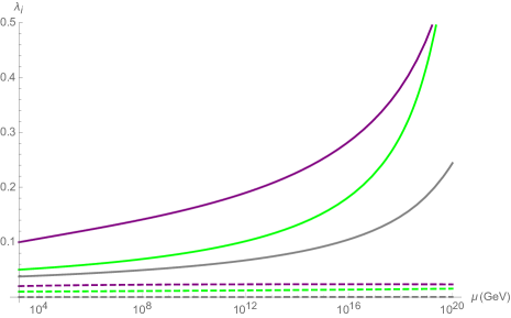
Figure 4: Upper panel: Shows the running of $\lambda_{1}$ (red), $\lambda_{2}$ (blue) and $\lambda_{3}$ (orange) above 1.7 TeV where the solid lines correspond to the upper bound on the combined $\lambda$ and the dashed lines are the lover bound. Lower panel: Shows the running of $\lambda_{4}$ (purple), $\lambda_{5}$ (green) and $\lambda_{\Omega}$ (grey) above 1.7 TeV where the solid lines are the upper bound on the combined $\lambda$ and the dashed lines are the lower bound.

In this case we can calculate the selfcouplings of the Higgs as we did in equation (16) in the previous section. However we find that they are independent of the extra scalar $\Omega$. In the allowed region in the parameter space we find the ratio of the trilinear couplings of the Higgs over the SM value:

$$1.32\cdot 10^{-3}<\frac{\lambda_{h_{1}h_{1}h_{1}}}{\lambda_{hhh}^{SM}}<2.43\cdot 10^{-3}\qquad\text{and}\qquad 18.2<\frac{\lambda_{h_{2}h_{2}h_{2}}}{\lambda_{hhh}^{SM}}<24.9.$$ (22)

V Conclusion

We have examined the running of the couplings for the model with a global symmetry breaking pattern $\mathrm{SO}(5)\to\mathrm{SO}(4)$, which is a minimal extension of the Standard Model, where the Higgs is an elementary pseudo Goldstone boson. We have considered the realization of the model in terms of elementary scalar fields, which is an appealing possibility: the model can be analysed with controllable perturbative calculations, and the model can in principle remain valid all the way up to the Planck scale analogously to what has been proposed to be the case for SM itself. However, when coupled to the electroweak currents, the model does not provide for a correct symmetry breaking pattern and vacuum properties Alanne:2016mmn . This issue can be solved in two different ways. We have separately analysed both of these possiblities to orient the vacuum in the desired and controllable way: First, by adding an explicit symmetry breaking term and second, adding instead an extra singlet scalar field.

To quantify the effects of the running of the couplings, we evaluated the beta functions of the three couplings in the pure $\mathrm{SO}(5)\to\mathrm{SO}(4)$ model. The pure doublet coupling depends strongly on the gauge and Yukawa couplings whereas the pure scalar coupling only depends indirectly on these. Adding an explicit breaking term does not change the beta functions and thereby the physical properties of the model.

On the other hand when adding a new scalar, three new couplings emerge and the three beta functions of the pure $\mathrm{SO}(5)\to\mathrm{SO}(4)$ model are slightly modified because of the interactions with the new singlet scalar. The new scalar self-coupling is similar to the original one as is also the case for the mixing of the new scalar with the doublet. The coupling between the new and the old scalar is slightly different from the scalar self-couplings but still it does not depend directly on the gauge and Yukawa couplings.

Our main result is that the mass intervals of the new heavy scalars are quite restricted by the overall constraints on the model. Below the renormalization scale we required the theory to reproduce the correct mass of the Higgs and above the renormalization scale we required the couplings to run in such a way, that the potential remains stable and the couplings remain perturbative all the way to the Planck scale. In both cases we analysed in this work we observed that the running of the couplings restricts the mass of the $\sigma$-particle to lie in a narrow interval, $M_{\sigma}\approx 3$ TeV with the reference renormalization scale to be around $\mu_{0}\approx 2$ TeV.

More detailed numbers are as follows: When we add an explicit breaking term, the mass lies in the interval $2.93\text{TeV}\leq M_{\sigma}\leq 3.10\text{TeV}$ and the related renormalization scale is $\mu_{0}\approx 1.7\,\text{TeV}$. When we add an extra scalar the interval of the mass is $2.81\text{TeV}\leq M_{\sigma}\leq 2.82\text{TeV}$ and the renormlization scale is $\mu_{0}\approx 2\,\text{TeV}$. The mass intervals do not overlap but are close to each other.

We have also compared the trilinear couplings for the Higgs particles and the heavier scalar state in both cases with the trilinear coupling of the SM. We found that the trilinear coupling of the light Higgs is three orders of magnitude smaller than the SM one and that the trilinear coupling of the heavy Higgs is one order of magnitude larger in both cases.

Based on these results, we can expect the models where the Higgs arises as an elementary pNGB to provide an interesting model building framework which can be viable up to the Planck scale. The difference with respect to the SM is the enlarged scalar sector and the dynamical emergence of the electroweak scale from symmetry breaking at significantly higher energies.

Appendix A Broken generators

First we identify $\mathrm{SU}_{L}(2)\times\mathrm{SU}_{R}(2)$ subgroup of $\mathrm{SO}(5)$ and fix the left and right generators as

$$\left(T_{\mathrm{L,R}}\right)_{ij}^{a}=-\frac{i}{2}\left[\frac{1}{2}\epsilon^{abc}\left(\delta^{b}_{i}\delta^{c}_{j}-\delta^{b}_{j}\delta^{c}_{i}\right)\pm\left(\delta_{i}^{a}\delta_{j}^{4}-\delta_{j}^{a}\delta_{i}^{4}\right)\right],$$ (23)

where the generator $T_{R}^{3}$ is identified with the generator of the hypercharge.

The broken generators for $\mathrm{SO}(5)\to\mathrm{SO}(4)$ are then

$$\begin{split}X^{1}_{ij}=&-i\left[\sin\theta\left(\delta_{i}^{1}\delta_{j}^{3}-\delta_{i}^{3}\delta_{j}^{1}\right)+\cos\theta\left(\delta_{i}^{1}\delta_{j}^{5}-\delta_{i}^{5}\delta_{j}^{1}\right)\right],\\ X^{2}_{ij}=&-i\left[\sin\theta\left(\delta_{i}^{2}\delta_{j}^{3}-\delta_{i}^{3}\delta_{j}^{2}\right)+\cos\theta\left(\delta_{i}^{2}\delta_{j}^{5}-\delta_{i}^{5}\delta_{j}^{2}\right)\right],\\ X^{3}_{ij}=&-i\left[-\sin\theta\left(\delta_{i}^{3}\delta_{j}^{4}-\delta_{i}^{4}\delta_{j}^{3}\right)+\cos\theta\left(\delta_{i}^{4}\delta_{j}^{5}-\delta_{i}^{5}\delta_{j}^{4}\right)\right],\\ X^{4}_{ij}=&-i\left(\delta_{i}^{3}\delta_{j}^{5}-\delta_{i}^{5}\delta_{j}^{3}\right).\end{split}$$ (24)

The generators are normalised such that $\text{Tr}[X^{a}_{\theta}X^{b}_{\theta}]=2\delta^{ab}$.

References

- (1) T. Asaka, S. Blanchet and M. Shaposhnikov, Phys. Lett. B 631, 151 (2005) doi:10.1016/j.physletb.2005.09.070 [hep-ph/0503065].
- (2) T. Asaka and M. Shaposhnikov, Phys. Lett. B 620, 17 (2005) doi:10.1016/j.physletb.2005.06.020 [hep-ph/0505013].
- (3) G. Degrassi, S. Di Vita, J. Elias-Miro, J. R. Espinosa, G. F. Giudice, G. Isidori and A. Strumia, JHEP 1208, 098 (2012) doi:10.1007/JHEP08(2012)098 [arXiv:1205.6497 [hep-ph]].
- (4) O. Antipin, M. Gillioz, J. Krog, E. Mølgaard and F. Sannino, JHEP 1308, 034 (2013) doi:10.1007/JHEP08(2013)034 [arXiv:1306.3234 [hep-ph]].
- (5) J. Elias-Miro, J. R. Espinosa, G. F. Giudice, G. Isidori, A. Riotto and A. Strumia, Phys. Lett. B 709, 222 (2012) doi:10.1016/j.physletb.2012.02.013 [arXiv:1112.3022 [hep-ph]].
- (6) A. Kobakhidze and A. Spencer-Smith, Phys. Lett. B 722, 130 (2013) doi:10.1016/j.physletb.2013.04.013 [arXiv:1301.2846 [hep-ph]].
- (7) M. Fairbairn and R. Hogan, Phys. Rev. Lett. 112, 201801 (2014) doi:10.1103/PhysRevLett.112.201801 [arXiv:1403.6786 [hep-ph]].
- (8) E. Gabrielli, M. Heikinheimo, K. Kannike, A. Racioppi, M. Raidal and C. Spethmann, Phys. Rev. D 89, no. 1, 015017 (2014) doi:10.1103/PhysRevD.89.015017 [arXiv:1309.6632 [hep-ph]].
- (9) K. Bhattacharya, J. Chakrabortty, S. Das and T. Mondal, JCAP 1412, no. 12, 001 (2014) doi:10.1088/1475-7516/2014/12/001 [arXiv:1408.3966 [hep-ph]].
- (10) M. Schmaltz and D. Tucker-Smith, Ann. Rev. Nucl. Part. Sci. 55, 229 (2005) doi:10.1146/annurev.nucl.55.090704.151502 [hep-ph/0502182].
- (11) S. R. Coleman and E. J. Weinberg, Phys. Rev. D 7, 1888 (1973). doi:10.1103/PhysRevD.7.1888
- (12) T. Alanne, H. Gertov, A. Meroni and F. Sannino, Phys. Rev. D 94 (2016) no.7, 075015 doi:10.1103/PhysRevD.94.075015 [arXiv:1608.07442 [hep-ph]].
- (13) T. Alanne, H. Gertov, F. Sannino and K. Tuominen, “Elementary Goldstone Higgs boson and dark matter,” Phys. Rev. D 91 (2015) 9, 095021 doi:10.1103/PhysRevD.91.095021 [arXiv:1411.6132 [hep-ph]].
- (14) H. Gertov, A. Meroni, E. Molinaro and F. Sannino, “Theory and phenomenology of the elementary Goldstone Higgs boson,” Phys. Rev. D 92 (2015) 9, 095003 doi:10.1103/PhysRevD.92.095003 [arXiv:1507.06666 [hep-ph]].
- (15) M. E. Machacek and M. T. Vaughn, “Two Loop Renormalization Group Equations in a General Quantum Field Theory. 1. Wave Function Renormalization,” Nucl. Phys. B 222 (1983) 83. doi:10.1016/0550-3213(83)90610-7
- (16) M. E. Machacek and M. T. Vaughn, “Two Loop Renormalization Group Equations in a General Quantum Field Theory. 2. Yukawa Couplings,” Nucl. Phys. B 236 (1984) 221. doi:10.1016/0550-3213(84)90533-9
- (17) M. E. Machacek and M. T. Vaughn, “Two Loop Renormalization Group Equations in a General Quantum Field Theory. 3. Scalar Quartic Couplings,” Nucl. Phys. B 249 (1985) 70. doi:10.1016/0550-3213(85)90040-9
- (18) K. Kannike, Eur. Phys. J. C 72 (2012) 2093 doi:10.1140/epjc/s10052-012-2093-z [arXiv:1205.3781 [hep-ph]].