Weak Lensing Peaks in Simulated Light-Cones: Investigating the Coupling between Dark Matter and Dark Energy

Abstract

In this paper, we study the statistical properties of weak lensing peaks in light-cones generated from cosmological simulations. In order to assess the prospects of such observable as a cosmological probe, we consider simulations that include interacting Dark Energy (hereafter DE) models with coupling term between DE and Dark Matter. Cosmological models that produce a larger population of massive clusters have more numerous high signal-to-noise peaks; among models with comparable numbers of clusters those with more concentrated haloes produce more peaks. The most extreme model under investigation shows a difference in peak counts of about $20\%$ with respect to the reference $\mathrm{\Lambda CDM}$ model. We find that peak statistics can be used to distinguish a coupling DE model from a reference one with the same power spectrum normalisation. The differences in the expansion history and the growth rate of structure formation are reflected in their halo counts, non-linear scale features and, through them, in the properties of the lensing peaks. For a source redshift distribution consistent with the expectations of future space-based wide field surveys, we find that typically seventy percent of the cluster population contributes to weak-lensing peaks with signal-to-noise ratios larger than two, and that the fraction of clusters in peaks approaches one-hundred percent for haloes with redshift $z\leq 0.5$. Our analysis demonstrates that peak statistics are an important tool for disentangling DE models by accurately tracing the structure formation processes as a function of the cosmic time.

1 Introduction

In the standard cosmological model, most of the energy in the Universe, approximately $70\%$, is in an unknown form, termed Dark Energy (hereafter DE) which has a negative pressure. This component is responsible for the late time accelerated expansion as measured by many observations (Perlmutter et al., 1999; Riess et al., 1998, 2004, 2007; Schrabback et al., 2010; Betoule et al., 2014). About $25\%$ of the energy content is in a different unknown component termed Dark Matter (DM), whose presence has been mainly inferred from its gravitational effects given that it seems not to emit nor absorb detectable levels of radiation (Zwicky, 1937; Rubin et al., 1980; Bosma, 1981a, b; Rubin et al., 1985).

Following the standard scenario, cosmic structures form as a consequence of gravitational instability. Dark matter overdensities contract and build up into so-called dark matter haloes (White & Rees, 1978; White & Silk, 1979). Small systems collapse first when the universe is denser and then merge together to form more massive objects (Tormen, 1998; Lacey & Cole, 1993, 1994). Galaxy clusters sit at the top of this hierarchy as the latest nonlinear structures to form in our Universe (Kauffmann & White, 1993; Springel et al., 2001b; Springel et al., 2005; Wechsler et al., 2002; van den Bosch, 2002; Wechsler et al., 2006; Giocoli et al., 2007).

The large amount of dark matter present in virialized systems and within the filamentary structure of our Universe is able to bend the light emitted by background objects (Bartelmann & Schneider, 2001). Because of this, the intrinsic shapes of background galaxies appear to us weakly distorted by gravitational lensing. Since lensing is sensitive to the total mass of objects and independent of how the mass is divided into the light and dark components of galaxies, groups and clusters, it represents a direct and clean tool for probing the distribution and evolution of structures in the Universe.

When light bundles emitted from background objects travel through high density regions like the centres of galaxies and clusters, the gravitational lensing effect is strong (SL): background images appear strongly distorted into gravitational arcs or divided into multiple images (Postman et al., 2012; Hoekstra et al., 2013; Meneghetti et al., 2013; Limousin et al., 2016). On the other hand, when light bundles transit the periphery of galaxies or clusters, background images are only slightly distorted and the gravitational lensing effect is termed weak (WL) (Amara et al., 2012; Radovich et al., 2015). In this way weak gravitational lensing represents an important tool for studying the matter density distributed within large scale structures. A large range of source redshifts allows one to tomographically probe the dark energy evolution through the cosmic growth rate as a function of redshift (Kitching et al., 2014; Köhlinger et al., 2016) (for a review see Kilbinger, 2014). Great efforts and impressive results have been reached by weak lensing collaborations like CFHTLens (Fu et al., 2008; Benjamin et al., 2013) and KiDS (Hildebrandt et al., 2017). Some tensions may still exist between these measurements and the ones coming from the Cosmic Microwave Background (Planck Collaboration et al., 2016). Hopefully, wide field surveys from space will help to fill the gap between low- and high-redshift cosmological studies and shed more light onto the dark components of our Universe.

Gravitational lensing will be the primary cosmological probe in several experiments that will start in the near future, like LSST (LSST Science Collaboration et al., 2009) and the ESA space mission Euclid (Laureijs et al., 2011). Recently, the Kilo Degree Survey (KiDS) collaboration presented a series of papers devoted to the shear peak analysis of $\sim 450$ deg² of data (Hildebrandt et al., 2017). They emphasised that peak statistics are a complementary probe to cosmic shear analysis which may break the degeneracy between the matter density parameter, $\Omega_{m}$, and $\sigma_{8}$, the power spectrum amplitude expressed in term of the root-mean-square of the linear density fluctuation smoothed on a scale of $8$ Mpc$/h$. In particular, Shan et al. (2017) analyzed the convergence maps reconstructed from shear catalogues using the non-linear Kaiser & Squires (1993) inversion (Seitz & Schneider, 1995). They showed that, given their source redshift distribution, peaks with signal-to-noise larger than three are mainly due to systems with masses larger than $10^{14}M_{\odot}/h$. However, the source distribution in the KiDS observations corresponds to a galaxy number density of only $7.5$ gal. per square arcmin at a median redshift of $z=0.6$. This low number density of galaxies prevented them from performing a tomographic analysis. Within the same collaboration, by using reconstructed maps from simulations, Martinet et al. (2017) confirmed the importance of combining peak and cosmic shear analyses. In particular they pointed out that cosmological constraints in the $\Omega_{m}$-$\sigma_{8}$ plane coming from low signal-to-noise peaks are tighter than those coming from the high-significance ones.

The strength of peak statistics in disentangling cosmological models has been discussed in the last years by several authors. In particular Maturi et al. (2011) have inspected the effect of primordial non-Gaussianity, which impacts the chance of projected large scale structures varying the peak counts. Pires et al. (2012) demonstrated that peak counts are the best statistic to break the $\sigma_{8}$-$\Omega_{m}$ degeneracy among the second-order weak lensing statistics. Reischke et al. (2016) have suggested that the extreme value statistic of peak counts can tighten even more the constraints on cosmological parameters.

In this work we will study weak lensing peak statistics in a sample of non-standard cosmological models which are characterised by a coupling term between dark energy and dark matter. We will discuss the complementarity of peak statistics with respect to cosmic shear and examine the information on non-linear scales from high significance peaks. We will discuss also the importance of tomographic analysis of peak statistics as tracers of the growth and the expansion history of the universe.

The paper is organised as follows: in Section 2 we present the numerical simulations analysed and introduce how weak lensing peaks have been identified. Statistical properties of peaks are reviewed in Section 3, while the connection between galaxy clusters and peaks is discussed in Section 4. We conclude and summarise in Section 5.

2 Methods and Numerical Simulations

2.1 Numerical Simulations of Dark Energy Models

In this work we use the numerical simulation dataset presented by (Baldi, 2012b) and partially publicly available at this url: http://www.marcobaldi.it/web/CoDECS_summary.html. The simulations have been run with a version of the widely used N-body code GADGET (Springel, 2005) modified by Baldi et al. (2010), which self-consistently includes all the effects associated with the interaction between a DE scalar field and $\mathrm{CDM}$ particles. The $\mathrm{CoDECS}$ suite includes several different possible combinations of the DE field potential – the exponential (Lucchin & Matarrese, 1985; Wetterich, 1988) or the $\mathrm{SUGRA}$ (Brax & Martin, 1999) potentials for example – and of the coupling function which can be either constant or exponential in the scalar field (see e.g. Baldi et al., 2011). For more details on the models we refer to Baldi (2012b).

In particular we use some simulations of the $\mathrm{L-CoDECS}$ sample ($\mathrm{\Lambda CDM}$, $\mathrm{EXP003}$, $\mathrm{EXP008e3}$ and $\mathrm{SUGRA003}$) plus $\mathrm{\Lambda CDM-HS8}$ that is a $\mathrm{\Lambda CDM}$ simulation with the same cosmological parameters as $\mathrm{\Lambda CDM}$ but with a value of $\sigma_{8}$ equal to the one of $\mathrm{EXP003}$. The $\mathrm{\Lambda CDM-HS8}$ simulation has been run in order to study how the effect of the coupling between DE and DM can be disentangled from a pure Cosmological Constant model with the same power spectrum normalisation. A summary of the considered simulations with their individual model parameters is given in Table 1

Table 1: The list of the cosmological models considered in the present work and their specific parameters. All the models have the same amplitude of scalar perturbations at $z_{\rm CMB}\approx 1100$, but have different values of $\sigma_{8}$ at $z=0$. In short, $\alpha$ is a parameter describing the slope of the scalar field potential, $\beta(\phi)$ is the coupling function describing the rate of energy-momentum exchange with dark matter, and $w_{\phi}(z=0)$ is the effective equation of state parameter ($p/\rho$). See Baldi (2012b) for details.

Model	Potential	$\alpha$	$\beta(\phi)$	$w_{\phi}(z=0)$	$\sigma_{8}(z=0)$
$\mathrm{\Lambda CDM}$	$V(\phi)=A$	–	–	$-1.0$	$0.809$
$\mathrm{\Lambda CDM-HS8}$	$V(\phi)=A$	–	–	$-1.0$	$0.967$
$\mathrm{EXP003}$	$V(\phi)=Ae^{-\alpha\phi}$	$0.08$	$0.15$	$-0.992$	$0.967$
$\mathrm{EXP008e3}$	$V(\phi)=Ae^{-\alpha\phi}$	$0.08$	$0.4\exp[3\phi]$	$-0.982$	$0.895$
$\mathrm{SUGRA003}$	$V(\phi)=A\phi^{-\alpha}e^{\phi^{2}/2}$	$2.15$	$-0.15$	$-0.901$	$0.806$

We also use the information about the halo catalogue computed for each simulation snapshot using a Fried-of-Friend (FoF) algorithm with linking parameter $b=0.2$ times the mean inter-particle separation. At each simulation snapshot, within each FoF group we also identify gravitationally bound substructures using the subfind algorithm (Springel et al., 2001b). subfind searches for overdense regions within a FoF group using a local SPH density estimate, identifying substructure candidates as regions bounded by an isodensity surface that crosses a saddle point of the density field, and testing that these possible substructures are physically bound with an iterative unbinding procedure. For both FoF and subfind catalogues we select and store systems with more than 20 particles, and define their centres as the position of the particle with the minimum gravitational potential. It is worth noting that while the subhaloes have a well-defined mass that is the sum of the mass of all particles belonging to them, different mass definitions are associated with the FoF groups. We define as $M_{\rm FoF}$ the sum of the masses of all particles belonging to the FoF group and as $M_{200}$ the mass around the FoF centre enclosing a density that is $200$ times the critical density of the universe at the corresponding redshift.

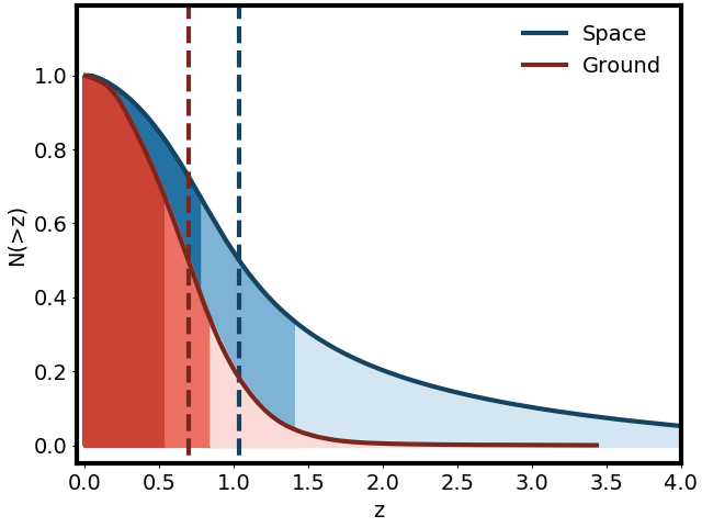
Figure 1: Cumulative normalised probability functions for two source redshift distributions, termed Space and Ground. While the Ground distribution has been build to match the source redshift distribution of CFHTLens (Kilbinger et al., 2013), the Space one corresponds to the distribution adopted by Boldrin et al. (2012, 2016) as expected from a wide field survey from space, like Euclid. The two dotted lines mark the median source redshifts in the two cases, while the different coloured regions below the curves indicate the redshift ranges in which one third of the galaxies are expected.

To compare the expected results for surveys from ground and space, we adopt in our analyses two different distribution functions of sources, shown in Fig. 1. The red (blue) curve, normalised to unity, mimics the probability distribution of sources as (expected to be) observed from ground (space) photometric survey. In particular the red curve corresponds to the redshift distribution from CFHTLens (Kilbinger et al., 2013), while the blue curve corresponds to the distribution adopted by Boldrin et al. (2012, 2016). The latter has been obtained using a simulated observation with the SkyLens code (Meneghetti et al., 2008; Bellagamba et al., 2012; Rasia et al., 2012) and identifying with SExtractor (Bertin & Arnouts, 1996) sources $3$ times above the background rms. The two dashed vertical lines, red and blue, mark the median redshift from ground and space, respectively. The regions shaded in three gradations of colour enclose the redshift ranges where we have one-third of the number density of sources for the two corresponding distributions. As can be seen, the source distribution from space moves toward higher redshifts with a considerable tail that extends beyond $z=2$: the expectations from space-based observations suggest a gain of at least a factor of two in the number of galaxies per square arcmin with measurable shapes. We reasonably assume a total number density of $18$ and $33$ galaxies per arcmin² for a ground and space experiment, respectively.

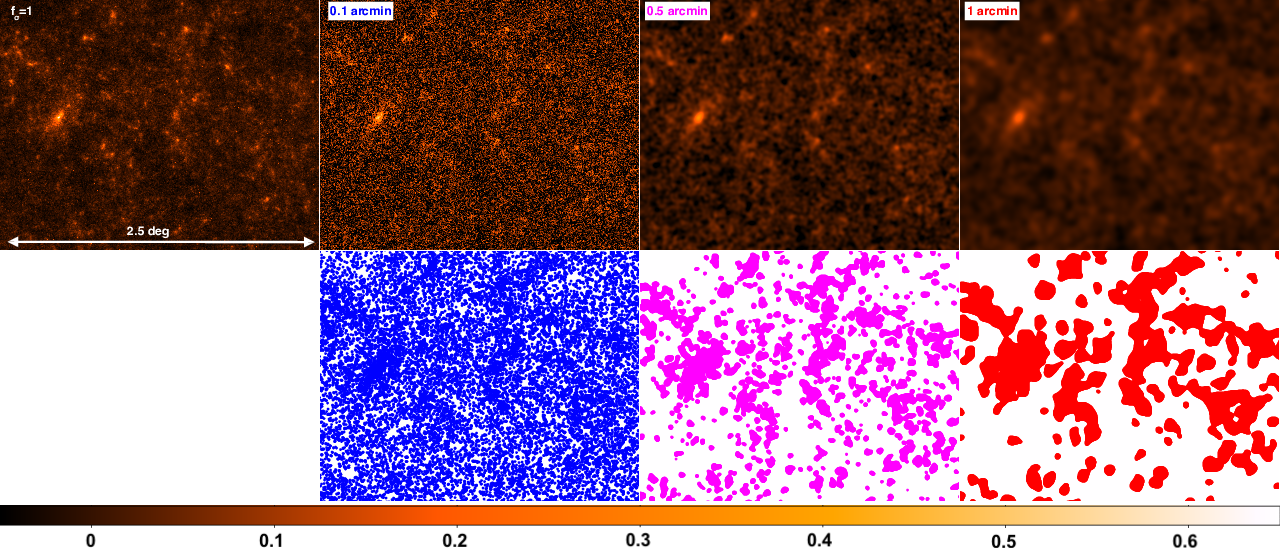
Figure 2: Noised and smoothed convergence maps considering different choices for the filter $\theta_{F}$. The top left panel shows the original convergence map. The other top panels, moving from left to right, display the convergence maps artificially noised and filtered considering $\theta_{F}$ $0.1$, $0.5$ and $1$ arcmin. The bottom sub-panels display the regions, in the corresponding maps, above the noise level.

2.2 Light-Cone Reconstruction and Peak Detection

We perform our weak lensing peak detection using convergence maps for different source redshifts and for various cosmological models. We employ the MapSim routine developed by Giocoli et al. (2015) to construct $25$ independent light-cones from the snapshots of our numerical simulations. We build the lens planes from the snapshots while randomising the particle positions by changing sign of the comoving coordinate system or arbitrarily selecting one of the nine faces of the simulation box to be located along the line-of-sight. If the light-cone reaches the border of a simulation box before it has reached a redshift range where the next snapshot will be used, the box is re-randomised and the light-cone extended through it again. The lensing planes are built by mapping the particle positions to the nearest pre-determined plane, maintaining angular positions, and then pixelizing the surface density using the triangular-shaped cloud method. The selected size of the field of view is $5\times 5$ sq. degrees and the maps are resolved with $2048\times 2048$ pixels, which corresponds to a pixel resolution of about 8.8 arcsec. Through the lens planes we produce the corresponding convergence maps for the desired source redshifts using the glamer code (Metcalf & Petkova, 2014; Petkova et al., 2014; Giocoli et al., 2016).

As done by Harnois-Déraps & van Waerbeke (2015b), for the lens planes stacked into the light-cones we define the natural source redshifts as those lying at the end of each constructed lens planes. By construction our light-cone has the shape of a pyramid where the observer is located at the vertex and the base extends up to the maximum redshift chosen to be $z=4$.

In wide field weak lensing analysis it is worth mentioning that intrinsic alignments (IAs) of galaxies may bias the weak lensing signal. However Shan et al. (2017) have shown that considering an Intrinsic Alignment (IA hereafter) amplitude as computed from the cosmic shear constraints by Hildebrandt et al. (2017), the relative contribution of IA to the noise variance of the convergence is very small and well bellow $0.6\%$ with respect to randomly oriented intrinsic ellipticities. Thus, to first approximation, we assume that the galaxies are intrinsically randomly oriented.

Noise can affect cosmological lensing measurements and results in possible biased constraints on cosmological parameters. One of the methods used to suppress the noise in reconstructed weak lensing fields is smoothing. Since weak gravitational lensing is by definition a weak effect, it is necessary to average over a sufficient number of source galaxies in order to obtain a measurement. Because of the central limit theorem, after smoothing the statistical properties of the noise field are expected to be close to a Gaussian distribution. For the noise and the characterisation of the convergence maps we follow the works of Lin & Kilbinger (2015a, b). The convergence maps $\kappa(x,y)$ that we produce from our ray-tracing procedure are only characterised by the discreteness of the density field sampled with collisionless particles: the so-called particle noise. However, to mimic the presence of galaxy shape noise, from which the convergence map is inferred from real observational data, we add to $\kappa(x,y)$ a noise field $n(x,y)$ that accounts for this. If we assume that the intrinsic ellipticities of the source galaxies are uncorrelated we can describe $n(x,y)$ as a Gaussian random field with variance:

$$\sigma_{\rm noise}^{2}=\dfrac{\sigma^{2}_{\epsilon}}{2}\dfrac{1}{2\pi\theta^{2}_{F}n_{g}}\;,$$ (1)

where $\sigma_{\epsilon}=0.25$ is the rms of the intrinsic ellipticity of the sources, $n_{g}$ the galaxy number density and $\theta_{F}$ represents the smoothing scale of a Gaussian window function filter, that we apply to the noised convergence map to suppress the pixel noise (Lin & Kilbinger, 2015a; Zorrilla Matilla et al., 2016; Shan et al., 2017). We indicate with $k_{n,F}$ the noised and filtered convergence map. Consistent with the choice made by other authors we adopt a scale of $1$ arcmin for the smoothing scale which represents the optimal size to isolate the contribution of massive haloes typically hosting galaxy clusters. For descriptive purposes, in the top left panel of Figure 2 we display the convergence map with an aperture of $2.5$ deg on a side and $z_{s}=1.12$. In the three panels on the left the noise has been added and the map has been smoothed assuming different choices of $\theta_{F}$, $0.1$, $0.5$ and $1$ arcminutes, from left to right, respectively. The coloured regions in the bottom panels mark the pixels in the image above that are above the noise level $f_{\sigma}=1$ with:

$$f_{\sigma}=\dfrac{\kappa_{n,F}}{\sigma_{\rm noise}}\,.$$ (2)

From the figure we can see that peaks identified in the convergence fields with small values of $\theta_{F}$ are dominated by false detections caused by the noise level. For larger $\theta_{F}$ values the peak locations consistently follow the locations of the interposed halos within the field-of-view.

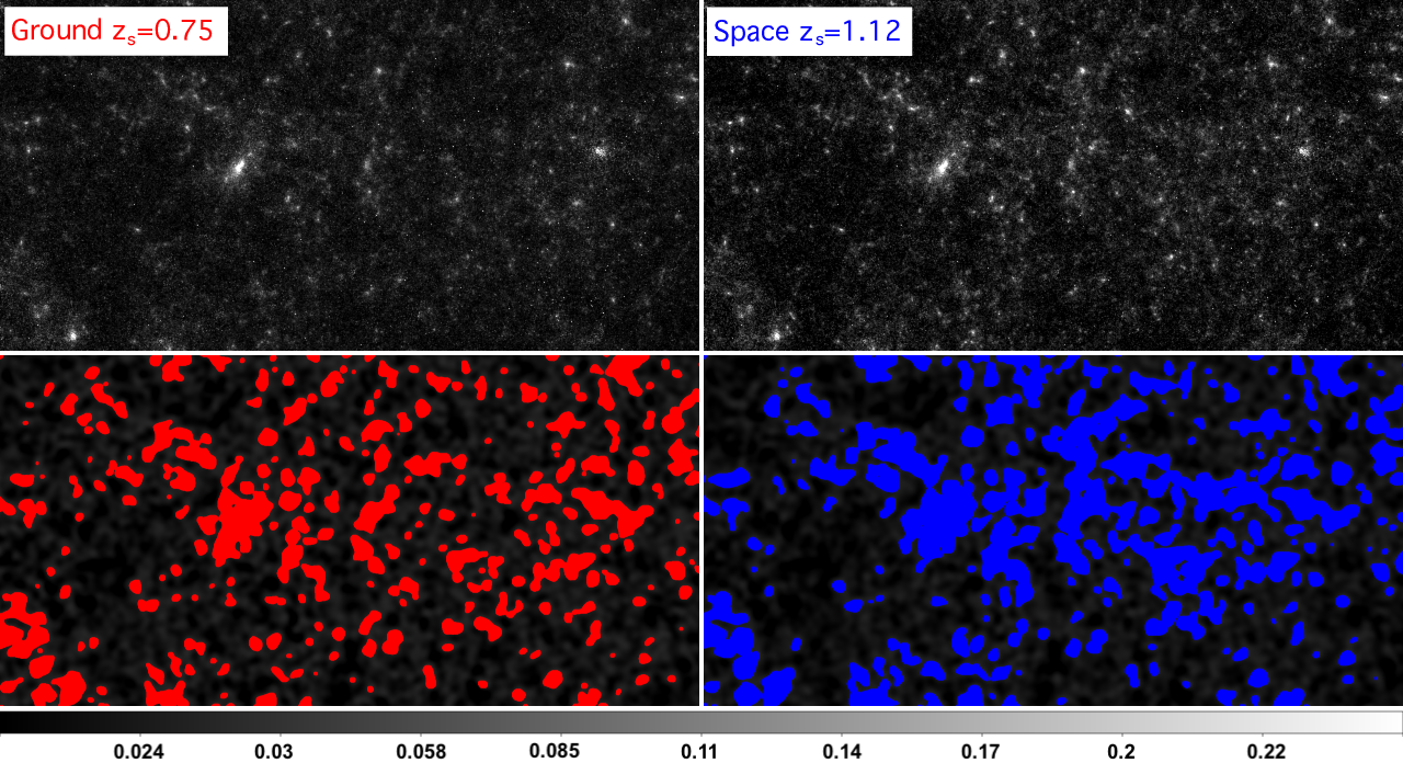
Figure 3: Top panels: convergence maps for one light-cone realisation of the $\mathrm{\Lambda CDM}$ simulation assuming sources at two fixed redshifts – corresponding to the median redshifts for the space- and ground-based redshift distributions here considered. Bottom panels: pixels above the corresponding noise level $\sigma_{\rm noise}$. The scale of the field-of-view along the x-axis of the displayed regions is approximately $3$ degrees large.

In our analysis we consider two natural source redshifts corresponding to $z_{s}=0.75$ and $z_{s}=1.12$ that are the medians of the two source redshift distributions as displayed in Fig. 1 . The top panels of Fig. 3 displays the convergence maps of a light-cone realisation from the $\mathrm{\Lambda}$CDM simulation considering these two source redshifts. The bottom panels shows the pixels in the corresponding maps $\kappa_{n,F}(x,y)$, noised and smoothed with $\theta_{F}=1$ arcmin to account for observational effects with $f_{\sigma}\geq 1$

We characterise the peak properties for a given threshold $f_{\sigma}$ as following: ($i$) we identify all the pixels above $f_{\sigma}$ times the noise level, ($ii$) we join them to the same peak group using a two-dimensional friend-of-friend approach adopting the pixel scale as linking length parameter, ($iii$) we define the coordinate of the peak centre according to the location of the pixel with the maximum value and the area as related to the number of pixels that belong to the group times the pixel area; we term our peak identification algorithm TwinPeaks: while for small values of the signal-to-noise threshold $f_{\sigma}$ some peaks are twins, for large values of $f_{\sigma}$ they become distinct and isolate. We want to emphasise that, as discussed, the peak identification method depends on the resolution of the convergence map – constructed from simulations or reconstructed using the shear catalogue of an observed field of view. Being interested in displaying and discuss relative differences in the counts and in the properties of the peaks for various Dark Energy models, all the maps have been created to have the same pixel resolution: field-of-view of $5$ deg by side are resolved with $2048\times 2048$ pixels, consistently noised and smoothed using the same parameter choices.

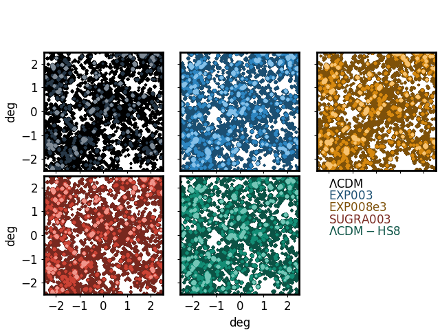
Figure 4: Examples of the weak lensing peak locations in the different cosmological models, from the map computed assuming a space source redshift distribution with $z_{s}=1.12$. The maps include shape noise and are smoothed with a Gaussian filter with scale $\theta_{F}=1$ arcmin. The different coloured panels show various cosmological models as indicated in the label. Within each panel the three gradations of colour mark the regions in the field-of-view which are $1$, $3$ and $5$ times above the expected noise level $\sigma_{\rm noise}$.

3 Weak Lensing Peak Properties in Coupled DM-DE Models

We run the complete and self-consistent TwinPeaks pipeline on all light-cones generated for the various cosmological models: $\mathrm{\Lambda CDM}$, $\mathrm{EXP003}$, $\mathrm{EXP008e3}$, $\mathrm{SUGRA}$ and $\mathrm{\Lambda CDM-HS8}$. In all cases we have considered two fixed source redshifts $z_{s}=0.75$ and $z_{s}=1.12$ (that are the median source redshifts of the two considered source redshift distributions) with a number density of galaxies of $18$ and $33$ per square arcmin for the ground- and space-based observations, respectively. As an example, in Figure 4 we display the TwinPeaks results for light-cones derived from the same random realisation of initial conditions at $z=99$ for the five different cosmological models, colour coded as displayed in the figure legend: black, blue, orange, red and green refer to $\mathrm{\Lambda CDM}$, $\mathrm{EXP003}$, $\mathrm{EXP008e3}$, $\mathrm{SUGRA003}$ and $\mathrm{\Lambda CDM-HS8}$, respectively. In this case, we show the results for $z_{s}=1.12$; in each panel the three gradations of colours mark the regions which are $1$, $3$ and $5$ times above the noise level, considering a filter size $\theta_{F}=1$ arcmin.

3.1 Peak Counts

Figure 5 displays the fraction of the area occupied by peaks as a function of the signal-to-noise level $f_{\sigma}$, for the various cosmologies. Each curve corresponds to the average value computed on the $25$ different light-cone realisations. Left and right panels display the results for a ground and space analysis, respectively. The outcomes for the various cosmological models are shown using different colours. The grey region bracketing the measurements of the $\mathrm{\Lambda CDM}$ model (black curve) shows the variance of the different light-cone realisations. The variance for the other models is similar and then not shown for clarity reasons. The corresponding bottom panels present the relative difference in the measured area in peaks with respect to the reference $\mathrm{\Lambda CDM}$ model as a function of the signal-to-noise value $f_{\sigma}$. The green diamonds show the predictions from our halo model formalism for the standard $\mathrm{\Lambda CDM}$ model, described in more details in the Appendix. We notice that the model describes quite well the predictions of the corresponding cosmological model, it captures within few percents the behaviour for large values of the signal-to-noise ratio. The blue crosses (present only on the right panel) show the results of our model where we also include the presence of subhaloes. As described by Giocoli et al. (2017) we treat them as Singular Isothermal Spheres. From a more detailed analysis we highlight that subhaloes boosts the weak lensing peaks at most $3$ percent. This is due to two main reasons: ($i$) subhaloes are typically embedded in more massive haloes whose contribution to the convergence map is stronger and ($ii$) their presence may be washed out by the noise and the smoothing of the convergence map. From the bottom panels we see that the higher peaks allow for a better discrimination between different cosmological models, while for low values of $f_{\sigma}$ the peaks trace mainly projected systems and filaments. At about $f_{\sigma}=6$ the two most extreme models EXP003 and $\mathrm{\Lambda CDM-HS8}$ show a positive difference of about $15-20\%$ while at $f_{\sigma}=10$ - attainable for a space observation with a large number density of background galaxies – of approximately $25-30\%$, in the regime where peaks are not dominated by the shape noise. The fraction of area in peaks for the EXP008e3 and SUGRA models are situated at almost $1$ $\sigma$ away from the $\mathrm{\Lambda CDM}$ one. It has also been pointed out by Maturi et al. (2010) who showed that weak-lensing peak counts are dominated by spurious detections up to signal-to-noise ratios of $3-5$ and that large scale structure noise can be suppressed using an optimised filter. For large $f_{\sigma}$ we detect the non-linear scales (typically for angular modes with $l>10^{2}$) where galaxy clusters are located, making peak statistic complementary to cosmic shear measurements (Shan et al., 2017). We can also see that observations from space should resolve peaks with a much higher resolution than ground-based ones and also resolve peaks with much higher signal-to-noise ratio where the difference between the various cosmological models is largest. Comparing the figure with the cosmic shear forecast analyses on the same cosmological models by Giocoli et al. (2015) we notice that high signal-to-noise peak statistics is able to differentiate more the various dark energy models. This suggests that future wide field surveys like Euclid will be excellent for this type of analyses, binding much more the cosmological models not only in the $\Omega_{m}$-$\sigma_{8}$ planes but also in the dark energy equation of state.

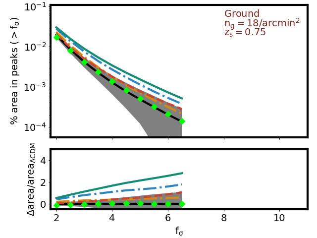
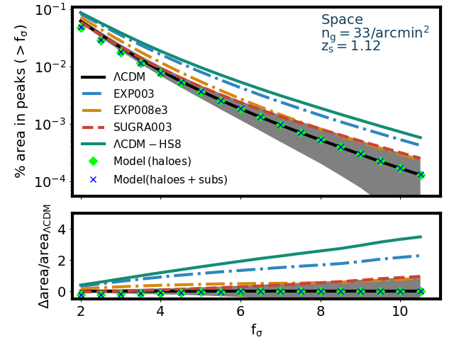
Figure 5: Left and right panels show the fraction of the area covered by weak lensing peaks as a function of the threshold of the noise level, for the various cosmological models for a space and a ground based source redshift distribution, respectively. The grey area bracketing the black lines shows the variance of the different light-cone realisations for the $\mathrm{\Lambda CDM}$ model. The various coloured curves display the measurement done on the light-cones of the different cosmological models. Green diamonds and blue crosses display the predictions obtained using our halo and halo plus subhalo models, discussed in the Appendix.

In Figure 6 we display the number of peaks above a given threshold of the signal-to-noise level; data points and colours are the same as in Fig. 5. From the figure we notice that the trend of the peak counts is very similar to that of the area in peaks as previously discussed. The $\mathrm{\Lambda CDM-HS8}$ is very distinct from the $\mathrm{\Lambda CDM}$ model in peak counts, showing also a different behaviour with respect to the $\mathrm{EXP003}$ model which has the same power spectrum normalisation. Peak statistics traces the different growth of structures and expansion histories. From the bottom panels we can notice that the $\mathrm{\Lambda CDM}$ model with high $\sigma_{8}$ predicts much more weak lensing peaks: this model has much more haloes which are much more concentrated due to their higher formation redshift. In general a higher peak abundance in weak lensing fields is mainly due to a combined effect of the projected halo mass function in the light-cones and to the redshift evolution of the mass-concentration relation.

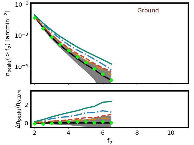
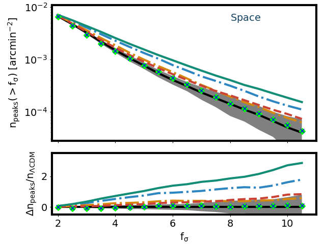
Figure 6: Peak counts above a given noise $f_{\sigma}$ level for the various cosmological models. Data points, lines and panels are as in Figure 5.

Results presented until now considered sources located at a fixed redshifts. However weak lensing tomographic analyses provide the possibility of tracing the structure formation process as a function of redshift and can be an important constraint on the growth factor and on the dark energy equation of state. This can be possible as long as we have a reasonable number of background galaxies per redshift bin. In order to perform a weak lensing peak analysis as a function of redshift, both for the space- and ground-based cases we divide the corresponding source redshift distribution in three redshift bins that contain one-third of the total expected number density of galaxies. As mentioned before those bins in redshift are displayed with different colour gradations in Figure 1. In Figure 7 we present the fraction of the area in peaks above a given threshold $f_{\sigma}=3$ as a function of the source redshift for the various cosmological models and the two experiments: from ground (left) and space (right): they have $6$ and $11$ galaxies per arcmin² per bin, respectively. For the space case we also show the measurement for high peaks with $f_{\sigma}=5$ (dashed lines), that are not properly resolved for the ground based experiment because of the low number density of background sources. The black error bar corresponds to the rms in the measurements for the reference $\mathrm{\Lambda CDM}$ model. The tomographic peak analysis illustrates the capability of following the structure formation processes for the different cosmological models. While for the ground-based case the maximum redshift considered is $z\approx 1.1$, from space we can go up to $z\approx 2.3$. As in the previous discussions both the EXP003 and $\mathrm{\Lambda CDM-HS8}$ present the largest differences in peaks with respect to the reference $\mathrm{\Lambda CDM}$ model. For example the right panel displays that the $\mathrm{SUGRA003}$ model has at high redshift an area in peaks very similar to the $\mathrm{\Lambda CDM}$ cosmology, while at low redshifts (as it can also be noticed in the left panel) the area in peaks is larger than the corresponding one in the standard model. This is actually consistent with the fact that $\mathrm{SUGRA003}$ is a bouncing model characterised by a different evolution of both the growth factor and the Hubble function (see Baldi, 2012a). Tomographic peak statistics will be a powerful tool for discriminating dark energy models from standard cosmological constant, being able to self-consistently trace the growth of structures, and more specifically – as we will discuss in the next section – of galaxy clusters as a function of the cosmic time.

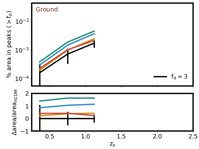
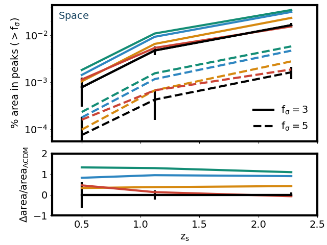
Figure 7: Fraction of the area in peaks as a function of the source redshift for space- (left) and ground-based (right) observations. Solid lines show the area above $3$ times the noise level, while the dashed ones consider peaks above $f_{\sigma}=5$. In particular for the ground-based experiment we display only the case for $f_{\sigma}=3$ since peaks with higher values of the noise are poorly resolved because of the number density of 8 galaxies per arcmin², per redshift bin. Various colours refer to the different cosmological models, as indicated in previous figures.

4 Galaxy Clusters and Weak Lensing Peaks

The results presented in the last section show that weak lensing peaks tend to be located close to high-density regions of the projected matter density distribution and that simulations based on the halo model describe quite well both the peak area and number counts as a function of the signal-to-noise ratio. The fact that the contribution of subhaloes to the weak lensing peaks is negligible also suggests that clusters, and line-of-sight projections of haloes, represent the main contribution to high peaks in the convergence maps.

In this section we will discuss the correlation between peaks and galaxy clusters present within the simulated light-cones, and try to shed more light on the connection between high peaks and massive haloes. We tag a halo as a contributor to a peak if its centre of mass has a distance smaller then $1$ pixel from a peak above a certain signal-to-noise value $f_{\sigma}$.

In Figure 8 we display the cumulative halo mass function per square degree within the constructed light-cones, for the various cosmological models, up to $z=0.75$, $z=1.12$ and $z=4$ from left to right, respectively. For the halo mass we use $M_{200}$, the mass enclosing $200$ times the critical density of the universe at the same redshift. For comparison, in each panel the light-blue and dark-grey curves display the predictions by Despali et al. (2016) and Tinker et al. (2008) for the $M_{200}$ mass definition. The bottom panels show the relative difference of the counts with respect to the measurement in the standard $\mathrm{\Lambda CDM}$ simulation. From these panels we can notice that the integrated halo mass function of the $\mathrm{SUGRA003}$ model is very similar to the $\mathrm{\Lambda CDM}$ (the $\mathrm{SUGRA003}$ model has been actually constructed to result in such similarity at low redshifts, see Baldi et al., 2011, for a detailed discussion on this issue). However the number of peaks in this model is quite different (as shown in Fig. 5 and 6) and comparable to the peak counts in EXP008e3. This is a clear signature of the halo properties (Cui et al., 2012; Giocoli et al., 2013): clusters in the bouncing $\mathrm{SUGRA003}$ model form at higher redshifts and are typically very concentrated. This translates in higher and more numerous peaks in the convergence field. This is a confirmation that peak statistics is very sensitive not only to the initial power spectrum but also to the non-linear processes that characterise halo formation histories and that may help disentangling models that would appear degenerate in other observables as the halo mass function. This is in agreement with the finding obtained by Shan et al. (2017): peak statistics gives complementary constraints with respect to cosmic shear in the $\sigma_{8}-\Omega_{m}$ plane, and in this case, as we have shown, also in the extended parameter space of coupled Dark Energy cosmologies.

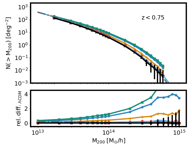
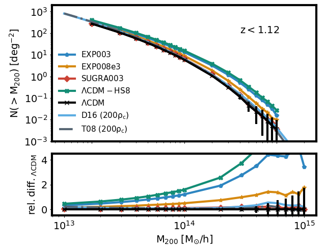
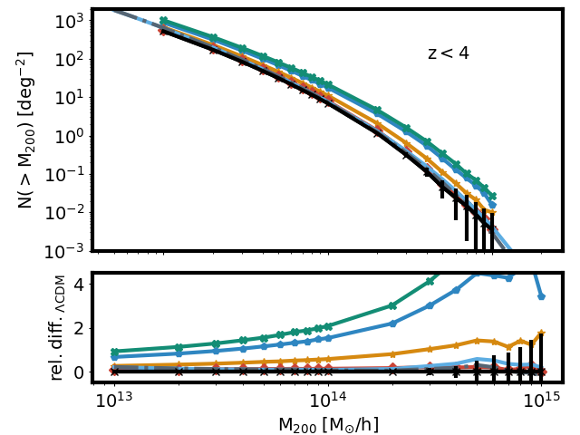
Figure 8: Halo mass function per square degree within the simulated light-cones up to redshifts $z=0.75$, $z=1.12$ and $z=4$ from left to right respectively. The data points show the measurements in the various cosmological models – with Poisson error bars displayed only for the $\mathrm{\Lambda CDM}$ model. The light-blue and dark-grey curves show the predictions from the Despali et al. (2016) and the Tinker et al. (2008) mass function for the $\mathrm{\Lambda CDM}$ cosmology.

The three panels in Figure 9 show the redshift distribution of clusters in the light-cones with mass $M_{200}\geq 10^{14}M_{\odot}/h$ as a function of redshift. Left and central panels display the redshift distribution of systems that fall into peaks with $f_{\sigma}=2$ for the ground- and space-based experiment, respectively; the right panel, instead, shows the distribution of the whole cluster population within the constructed past-light-cones. Dashed and solid vertical lines mark $z_{s}=0.75$ and $z_{s}=1.12$, respectively. In these figures it is possible to see that the number of clusters in the $\mathrm{SUGRA003}$ model is quite similar to $\mathrm{\Lambda CDM}$ one while large differences are present in the counts with respect to the $\mathrm{\Lambda CDM}$ with high $\sigma_{8}$ and $\mathrm{EXP003}$.

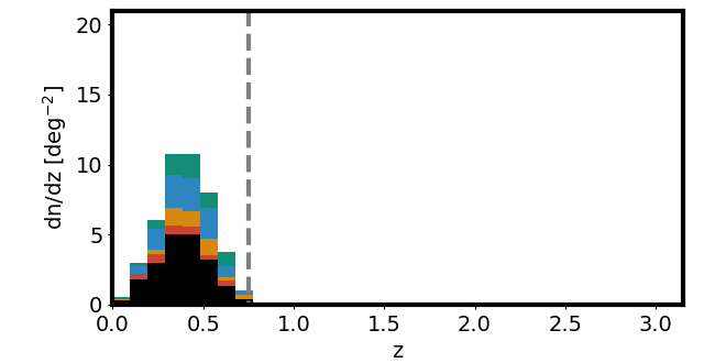
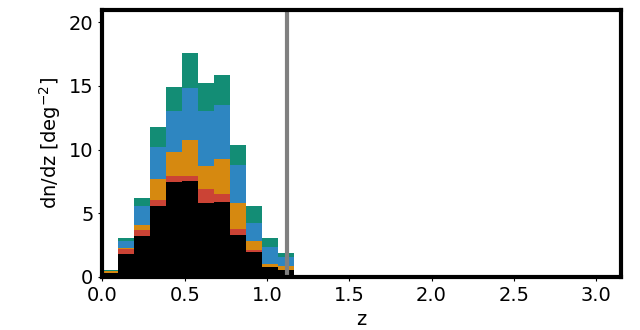
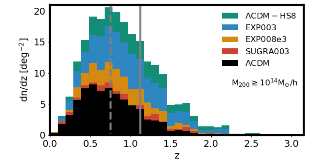
Figure 9: Differential number density of clusters with $M_{200}\geq 10^{14}M_{\odot}/h$ per unit of square degree for the various cosmological models. Left and central panels show the redshift distributions of clusters in peaks with $f_{\sigma}=2$ for the ground and space experiments, respectively. Right panel displays the redshift distribution of clusters for each cosmological model within our constructed light-cones. Solid and dashed vertical lines show the source redshift for the two considered cases ground and space-based: $z_{s}=0.75$ and $z_{s}=1.12$, respectively.

Top and bottom panels in Figure 10 display the fraction of clusters corresponding to weak lensing peaks for space- and ground-based experiments, respectively. In both panels we show the fraction of clusters in peaks above various weak lensing noise levels, for the different cosmological models, colour coded as in the other figures. The considered source redshifts for the space- and ground-based experiments are $z_{s}=0.75$ and $z_{s}=1.12$, respectively, and that those also correspond to the maximum cluster redshift we consider; moreover we consider clusters with masses above $M_{200}\geq 10^{14}M_{\odot}/h$. We notice that for the space experiment we find that almost $55\%$ ($70\%$) of the clusters with $z<1.12$ are in peaks $3$ ($2$) times above the noise level, while for the ground-based experiment it is nearly $30\%$ ($50\%$) of all clusters with $z<0.75$. We remind the reader that for a cluster to be within a peak it is necessary that its projected centre of mass falls in a pixel of the corresponding map that is above the desired threshold: by definition each peak, depending on its shape, may or not contain more than a halo with $M_{200}\geq 10^{14}M_{\odot}/h$. The halo contribution to the corresponding weak lensing field is weighted by the lensing distance $D_{lens}\equiv D_{ls}D_{l}/D_{s}$ (where $D_{l}$ $D_{s}$ and $D_{ls}$ are the angular diameter distances observer-lens, observer-source and source-lens, respectively) so that haloes, even if they have the same mass, contribute differently to the lensing signal depending on their redshift: for example, considering $z_{s}=1.12$ the lensing distance $D_{lens}$ peaks around $z=0.38$. This is more evident in Figure 11 where we show the fraction of clusters with $z\leq 0.5$ in peaks above different thresholds of the noise level, for the space case. The fraction of haloes with $M_{200}\geq 10^{14}M_{\odot}/h$ and $z\leq 0.5$ in peaks with $f_{\sigma}=2$ is close to unity. The arrow on each data point shows the corresponding fraction of clusters in peaks when we select systems with $z\leq 0.38$ – the peak of the lensing kernel for $z_{s}=1.12$.

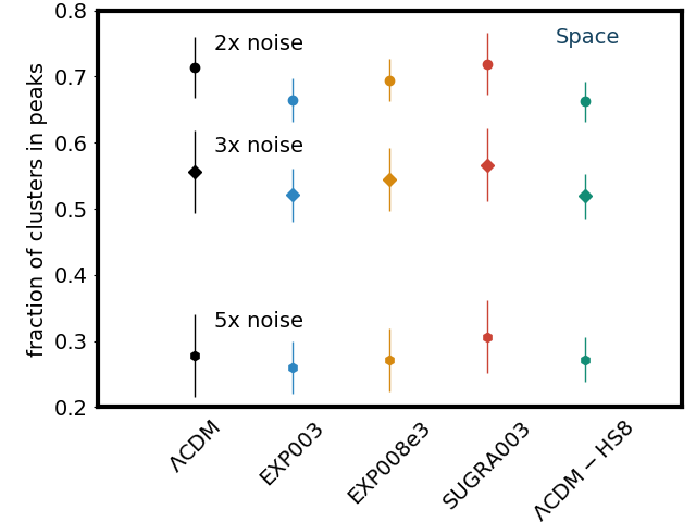
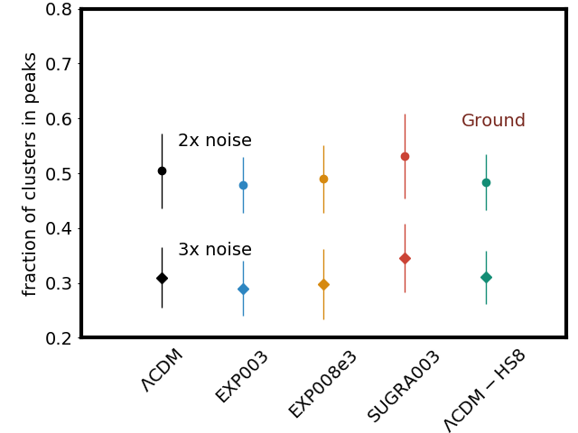
Figure 10: Fraction of clusters in peaks for a space- and ground-based analysis of the weak lensing simulations (top and bottom panel respectively) for the various cosmological models considered in this work. In the top panel we consider all the clusters with $M_{200}\geq 10^{14}M_{\odot}/h$ up to the source redshift of $z_{s}=1.12$, while in the bottom panel up to $z_{s}=0.75$. Different data points display the fractions of those systems whose centre of mass falls within high convergence pixels which are part of weak lensing peaks above a given threshold value $f_{\sigma}$.

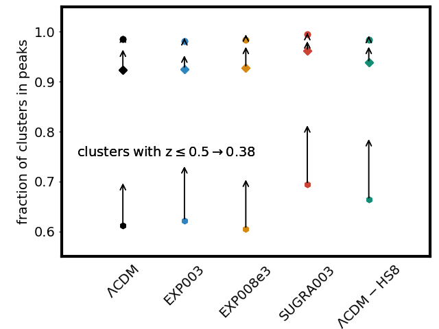
Figure 11: Fraction of clusters for a space-based analysis with $M_{200}\geq 10^{14}M_{\odot}/h$ and $z\leq 0.5$ in peaks with convergence values above $f_{\sigma}=2$, $3$ and $5$ from top to bottom data points, respectively. The arrow on each data point shows the corresponding fraction of clusters in peaks when we select systems with $z\leq 0.38$ – the peak of the lensing kernel for $z_{s}=1.12$.

Table 2: Number of clusters with $M_{200}\geq 10^{14}M_{\odot}/h$ (with $z<1.12$, second and third columns, and $z\leq 0.5$, forth and fifth columns) in peaks above the threshold of $f_{\sigma}=2$ in the various cosmological models. Second and fourth columns display the number of clusters in the various models up to redshift $1.12$ and $0.5$, respectively. On the other side, third and fifth columns present the corresponding cluster counts in peaks with signal-to-noise ratio $f_{\sigma}=2$, while the number between parentheses refers to the number of clusters in peaks for which the centre of mass corresponds with the pixel with the highest value. Numbers refer to the sum over $25$ different light-cone realisations, for a total of $625$ sq. deg., for each cosmology.

	n. cl. $z<1.12$ $\rightarrow$	n. cl. in peaks (with $\Delta\theta_{\rm cl,peak}=0$)	||	n. cl. $z\leq 0.5$ $\rightarrow$	n. cl. in peaks (with $\Delta\theta_{\rm cl,peak}=0$)
$\mathrm{\Lambda CDM}$	$3730$	2655 (90)	||	1207	1188 (53)
$\mathrm{EXP003}$	8223	5460 (158)	||	2130	2088 (83)
$\mathrm{EXP008e3}$	5523	3834 (102)	||	1602	1576 (57)
$\mathrm{SUGRA003}$	4069	2926 (130)	||	1314	1308 (77)
$\mathrm{\Lambda CDM-HS8}$	9684	6410 (191)	||	2429	2391 (110)
Model	3730	2634 (124)	||	1207	1201 (69)

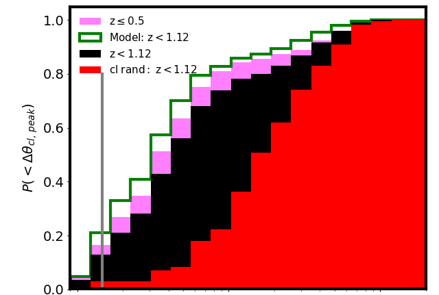
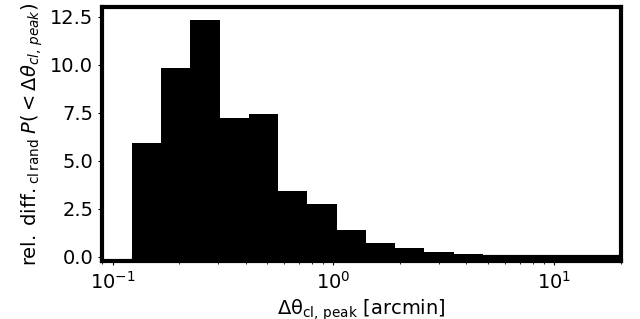
Figure 12: Normalised cumulative distribution of the distance between the centre of mass of the clusters in peaks and the closest pixel with highest value. The results refer to the $\mathrm{\Lambda CDM}$ cosmology. This result does not have important cosmological dependence, all the other models possess a similar distribution. The vertical grey line indicates the angular scale corresponding to the pixel size in the convergence map. The green histogram refers to the measurements with respect the convergence maps constructed using our fast weak lensing halo model formalism, discussed in details in the Appendix. The red histogram shows the cumulative distribution of the distance between peaks and clusters, when the latter are assumed to have random position within the field-of-view. The bottom panel displays the relative difference between the black and the red histograms.

The correlation between weak lensing peaks (above a given threshold) and clusters represents a promising statistics to identify regions in the plane of the sky where clusters are more likely to be found. In Figure 12 we display the normalised cumulative distribution of the angular distances $\Delta\theta_{\rm cl,peak}$ between the cluster centre of mass and the location of the closest pixel with the highest value of the convergence with $f_{\sigma}=2$. The black shaded histogram shows the cumulative distribution of distances $\Delta\theta_{\rm cl,peak}$ in arcmin for the $\mathrm{\Lambda}$CDM light-cones for sources and clusters up to $z=1.12$, while the green lines refers to the halo model predictions when weak lensing maps are produced using our fast weak lensing model (see Appendix). The relative difference between those two histograms remains well below $10\%$ and both distributions converge to unity around $7$ arcmin. Nonetheless, peaks in the convergence maps created using all the particles from the simulations have slightly misaligned centres and less correlation with cluster centres than peaks in the halo model maps because of the filamentary structure present in the convergence field. This manifests also in the fact that peaks are not spherical but typically elliptical. The magenta histogram displays the case of clusters with $z\leq 0.5$, that, as we will discuss later, contribute the most to the convergence peaks with $f_{\sigma}=2$ and $z_{s}=1.12$. The vertical grey line indicates the angular scale of the pixel of the convergence maps. From the figure we notice that less than five percent of the clusters have a centre of mass that overlaps with the highest peak, approximately seventy percent are closer than one arcmin to the highest peak while all clusters are within $7$ arcmin from some peak. In order to see how the correlation between clusters and peaks compares with respect to random points, in red we display the cumulative distribution of the distance between clusters and peaks, when the former are assumed to have random positions within the field-of-view. The relative difference between the two distributions clusters-peaks and random clusters-peaks (black and red histograms, respectively) is displayed in the bottom panel. In this panel we can notice in more details that at small scales clusters and peaks are more correlated than random cluster positions which has a maximum at about $15$ arcsec.

In Table 2 we summarise our results about the correspondence of weak lensing peaks and clusters within the simulated past light-cones. Each row refers to a different cosmological model, while the last one reports the findings in our halo model simulated fields for the $\mathrm{\Lambda CDM}$ cosmology. The numbers correspond to the $25$ different light-cone realisations for each model for a total of $625$ square degrees.

5 Summary & Conclusions

In this work we have investigated the weak lensing peak statistics and properties in a set of light-cones constructed from the coupled DM-DE simulations of the $\mathrm{CoDECS}$ suite. In particular we have studied how the number density and area of weak lensing peaks differ between models using typical source redshift distribution from ground and space observations. In what follows we summarise our main findings:

• the various cosmological models display different peak counts that increase with the signal-to-noise ratio $f_{\sigma}$. The extreme model $\mathrm{EXP003}$ for $f_{\sigma}=10$ displays a relative difference of about $20\%$ with respect to the $\mathrm{\Lambda CDM}$ and exhibits a different behaviour with respect to the $\mathrm{\Lambda CDM-HS8}$ which has the same power spectrum normalisation;

• the fraction of area on the sky in peaks as a function of the signal-to-noise ratio displays a behaviour similar to that of the peak counts, except that for small values of $f_{\sigma}$ we found twin-peaks above a given threshold while for large values of $f_{\sigma}$ high convergence regions are isolated and become more distinct with respect to the projected linear and non-linear large scale matter density distribution; the relative difference between $\mathrm{EXP008e3}$ and $\mathrm{SUGRA003}$ in peak area is reversed with respect to peak counts underlining the importance of the concentration-mass relation in peak statistics;

• weak lensing peaks reflect the non-Gaussian properties of the underlying projected density field, trace non-linear structure formation processes and are very sensitive to the evolution of dark energy through the growth of density perturbations and the geometry of the expansion history. This confirms the idea that weak lensing peak statistics, and their tomographic analysis, can provide complementary information to cosmic shear analysis alone;

• peak abundance and properties are due to non-linear structures present along the line-of-sight and projected matter density distribution; in particular high signal-to-noise peaks are mainly produced by galaxy clusters and for the source redshift distribution as expected from a space-based experiment we find that almost the whole cluster population up to $z=0.5$ is in peaks with signal-to-noise ratio $f_{\sigma}=2$;

• only five percent of the clusters have their centres of mass within the highest pixel in a peak of the convergence map (resolution $8.8$ arcsec). On the other hand, all clusters are located within $7$ arcminutes of the maximum convergence pixel of a peak;

• our halo model formalism for creating fast weak lensing simulations describes well the abundance of peaks for the different source redshift distributions;

• the inclusion of substructures in our halo model raises the peak statistics only by a few percent;

Weak lensing peak statistics represents a powerful tool for characterising non-Gaussian properties of the projected matter density distribution. Peak properties depend on dark energy and their tomographic analysis allows one to trace the structure formation processes as a function of the cosmic time. Our results underline the necessity of combining peak statistics with other cosmological probes: this will offer important results from upcoming wide field surveys and will push cosmological studies toward new frontiers.

Appendix A Fast Halo Model Simulations and a Model for Weak Lensing Peaks

Modelling peak statistics represents a significant challenge when using peak counts as complementary cosmological probe to cosmic shear power spectrum. Predicting peaks in weak lensing convergence maps can be done assuming that non-linear structures, like dark matter haloes, are the main contributors to high-significance peaks. In this paper we have shown that while haloes hosting galaxy clusters are the main contributors to high peaks, projection effects from small haloes aligned along the line-of-sight contribute to peaks with low signal-to-noise ratio.

In this appendix we will show that peaks identified in convergence maps constructed using fast weak lensing simulations with WL-MOKA (Giocoli et al., 2017) are in very good agreement with those in maps computed from full particle ray-tracing simulations. Fast halo model simulations could prove extremely useful by reducing the computational requirements for N-body simulations by some orders of magnitude both in cosmic shear power spectrum and peak statistics (Lin & Kilbinger, 2015a, b; Zorrilla Matilla et al., 2016) when combined with approximate simulation methods like COLA (Izard et al., 2018) and PINOCCHIO (Monaco et al., 2013; Munari et al., 2017; Monaco, 2016). As discussed by Giocoli et al. (2017) on a single light-cone simulation, our fast halo model method is approximately $90$ per cent faster than a full ray-tracing simulation using particles. However, it should be stressed that an N-body run of $1$ Gpc/$h$ with $1024^{3}$ collisionless particles from $z=99$ to the present time using the GADGET2 code (Springel, 2005) takes around $50$ $000$ CPU hours, while a run with an approximate method may take approximately $750$ CPU hours to generate the past-light cone up to the desired maximum redshift $z=4$.

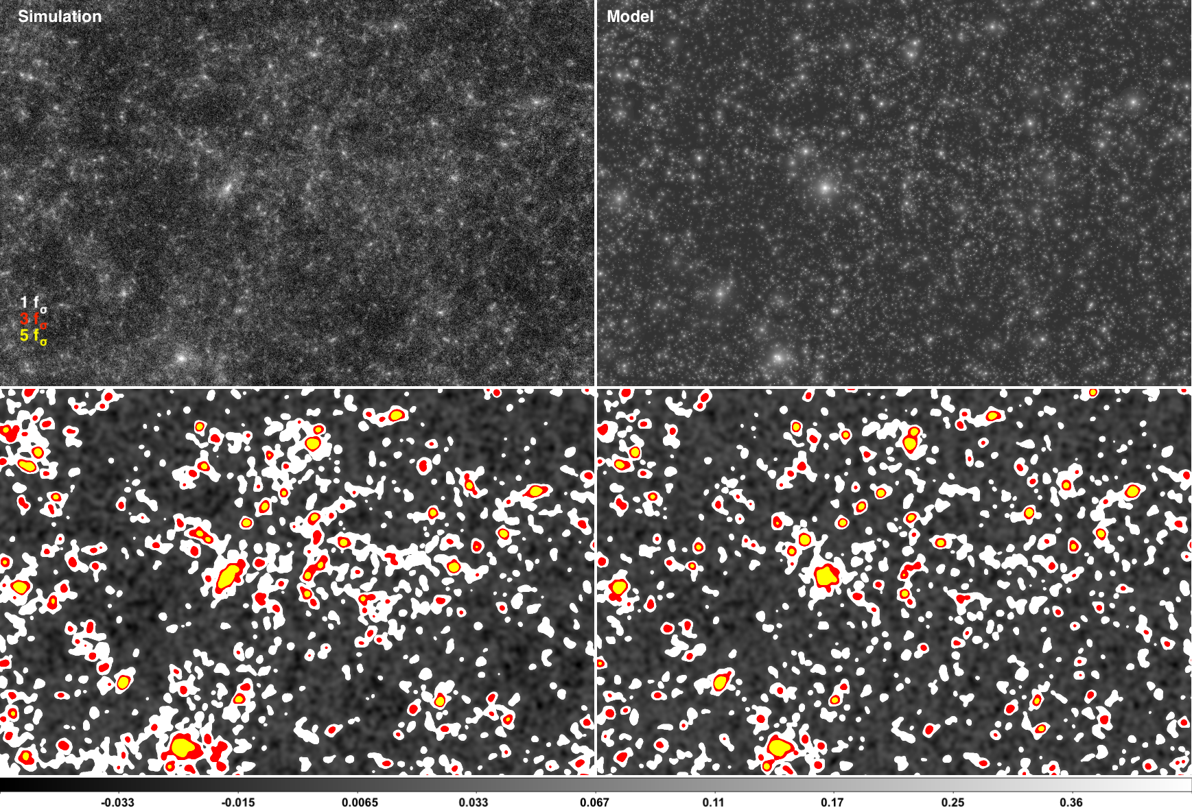
Figure 13: Top panels: convergence maps for source redshift $z_{s}=1.12$. In the left panel we show the map computed using all particles within the light-cone while on the right we display the reconstruction performed using all haloes with friends-of-friends mass larger than $2.1\times 10^{12}M_{\odot}/h$. Bottom panels: peak detection in convergence maps created using particles (left) and haloes (right) from the same light-cone realisation of the $\mathrm{\Lambda CDM}$ simulation. The convergence map has been constructed assuming $z_{s}=1.12$, noised and smoothed assuming $\sigma_{F}=1$ arcmin and $33$ galaxies per square arcmin. In white, red and yellow we display the pixels in the map which are $1$, $3$ and $5$ times above the noise level.

The theoretical approach for weak lensing peak prediction is based on the projected halo model formalism (Cooray & Sheth, 2002). A full characterisation of the halo population along the line-of-sight, with consistent clustering properties, gives us the possibility of predicting not only the peaks in cluster regions but also those in the field , mainly due to projected interposed mass density distribution.

In order to build our peak model, in addition to the convergence maps constructed using the particles from the numerical simulations, for the $\mathrm{\Lambda CDM}$ model we also use a sample of maps computed using the halo properties as presented in Giocoli et al. (2017). In order to do so, we use the corresponding projected halo and subhalo catalogue from MapSim, considering all friends-of-friends groups above the resolution $M>2.1\times 10^{12}M_{\odot}/h$. Each halo, as read from the simulation catalogue and present within the considered light-cone field-of-view, is assumed to be spherical and characterised by a well defined density profile (Navarro et al., 1996) (hereafter NFW). We assume the halo concentration $c$ to be mass and redshift dependent as in Zhao et al. (2009) in which we imply the mass accretion history model by Giocoli et al. (2012b) and we assume a log-normal scatter in concentration for fixed halo mass of $\sigma_{\ln c}=0.25$ consistent with the results of different numerical simulations (Jing, 2000; Dolag et al., 2004; Sheth & Tormen, 2004; Neto et al., 2007). In this case we can compute the convergence map by integrating the halo profile along the line-of-sight up to the virial radius that can be read as:

$$\kappa(x,y)=\int_{-R_{vir}}^{R_{vir}}\rho(x,y,z)\mathrm{d}z/\Sigma_{\rm crit}\,,$$ (3)

where

$$\Sigma_{cr}\equiv\frac{c^{2}}{4\pi G}\frac{1}{D_{lens}}$$ (4)

is the critical surface mass density. For the NFW profile and assuming that along the line-of-sight we can integrate up to infinity, equation (3) can be simplified to (Bartelmann, 1996):

$$\kappa_{NFW}(x,y)=\frac{2\rho_{s}r_{s}}{\zeta^{2}-1}\dfrac{F(\zeta)}{\Sigma_{\rm crit}}\,,$$ (5)

where $\zeta\equiv\sqrt{(}x^{2}+y^{2})/r_{s}$, $r_{s}=R_{vir}/c$, and:

$$F(\zeta)=\left\{\begin{array}[]{ll}1-\frac{2}{\sqrt{\zeta^{2}-1}}\arctan\sqrt{\dfrac{\zeta-1}{\zeta+1}}&\zeta>1,\\ 1-\frac{2}{\sqrt{1-\zeta^{2}}}\mathrm{arctanh}\sqrt{-\dfrac{\zeta-1}{\zeta+1}}&\zeta<1,\\ 0&\zeta=1.\\ \end{array}\right.$$

Left and right panels of Fig. 13 show the convergence maps for $z_{s}=1.12$ of one light-cone realisation of the $\mathrm{\Lambda CDM}$ model using particles and haloes, respectively. The top panels show the convergence maps for $z_{s}=1.12$ while in the bottom we have includeed random noise assuming a number density of galaxies $n_{g}=33$ arcmin^-2 and the maps have been convolved with a Gaussian filter with $\sigma_{F}=1$ arcmin. In white, red and yellow we display the regions in the maps that are $1$, $3$ and $5$ times above the noise level. From the figure we notice that qualitatively the peak location is very similar: the most massive haloes are responsible for the highest convergence peaks, regions with few systems appear, in projection, under-dense. However the shapes of the peaks in the right panel are quite spherical as the haloes used in the construction are, however the halo locations correlate with the peaks as well as with the large scale matter density distribution (Despali et al., 2014; Bonamigo et al., 2015; Despali et al., 2017).

In producing the lensing simulation model using haloes we have been consistent in taking the halo positions from the simulation, and projecting them on the plane of the sky. This means that up to the simulation scale of $1$ Gpc/$h$ the clustering of the systems is preserved. However one may ask if this has a direct impact on the peak counts of the constructed convergence maps. In order to understand this for each halo model light-cone we have created 16 realisations where we have preserved the halo masses and concentrations but we have assigned to each halo a random position within the field of view. In Figure 14 we display the relative number counts and area in peaks as a function of the signal-to-noise level $f_{\sigma}$ between the halo model simulation when positions are read from the simulation and when they are randomly assigned. We show the results both for a space- and ground-based analysis displayed in blue and red, respectively. The figure shows that proper halo positions are necessary for a good characterisation of the peak statistics mainly for high values of the noise level. These allow a good description of the large scale density distribution and of the effect of correlated and uncorrelated structures on the location of high density regions. From the figure we can see that for large values of the noise level the relative difference in the area and in the number of peaks tends to $10\%$ and that in the upper panel already for $f_{\sigma}=2$ the relative difference is about $5\%$.

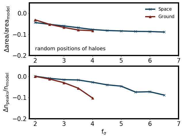
Figure 14: Relative peak area and counts as a function of the noise threshold, from our fast lensing halo model, when the halo positions are read from the simulation and defined to be random. The red and blue data points show the results considering a space or a ground based analysis, respectively.

References

- Amara et al. (2012) Amara A., Lilly S., Kovač K., Rhodes J., Massey R., Zamorani G., Carollo et al. 2012, MNRAS, 424, 553
- Baldi (2012a) Baldi M., 2012a, Physics of the Dark Universe, 1, 162
- Baldi (2012b) Baldi M., 2012b, MNRAS, 422, 1028
- Baldi et al. (2011) Baldi M., Pettorino V., Amendola L., Wetterich C., 2011, MNRAS, 418, 214
- Baldi et al. (2010) Baldi M., Pettorino V., Robbers G., Springel V., 2010, MNRAS, 403, 1684
- Bartelmann (1996) Bartelmann M., 1996, A&A, 313, 697
- Bartelmann & Schneider (2001) Bartelmann M., Schneider P., 2001, Physics Reports, 340, 291
- Bellagamba et al. (2012) Bellagamba F., Meneghetti M., Moscardini L., Bolzonella M., 2012, MNRAS, 422, 553
- Benjamin et al. (2013) Benjamin J., Van Waerbeke L., Heymans C., Kilbinger M., Erben T., Hildebrandt H., Hoekstra H., et al. 2013, MNRAS, 431, 1547
- Bertin & Arnouts (1996) Bertin E., Arnouts S., 1996, A&AS, 117, 393
- Betoule et al. (2014) Betoule M., Kessler R., Guy J., Mosher J., Hardin D., Biswas R., Astier P., et al. 2014, A&A, 568, A22
- Boldrin et al. (2012) Boldrin M., Giocoli C., Meneghetti M., Moscardini L., 2012, MNRAS, 427, 3134
- Boldrin et al. (2016) Boldrin M., Giocoli C., Meneghetti M., Moscardini L., Tormen G., Biviano A., 2016, MNRAS, 457, 2738
- Bonamigo et al. (2015) Bonamigo M., Despali G., Limousin M., Angulo R., Giocoli C., Soucail G., 2015, MNRAS, 449, 3171
- Bosma (1981a) Bosma A., 1981a, AJ, 86, 1791
- Bosma (1981b) Bosma A., 1981b, AJ, 86, 1825
- Brax & Martin (1999) Brax P. H., Martin J., 1999, Physics Letters B, 468, 40
- Cooray & Sheth (2002) Cooray A., Sheth R., 2002, Physics Reports, 372, 1
- Cui et al. (2012) Cui W., Baldi M., Borgani S., 2012, MNRAS, 424, 993
- Despali et al. (2016) Despali G., Giocoli C., Angulo R. E., Tormen G., Sheth R. K., Baso G., Moscardini L., 2016, MNRAS, 456, 2486
- Despali et al. (2017) Despali G., Giocoli C., Bonamigo M., Limousin M., Tormen G., 2017, MNRAS, 466, 181
- Despali et al. (2014) Despali G., Giocoli C., Tormen G., 2014, MNRAS, 443, 3208
- Dolag et al. (2004) Dolag K., Bartelmann M., Perrotta F., Baccigalupi C., Moscardini L., Meneghetti M., Tormen G., 2004, A&A, 416, 853
- Fu et al. (2008) Fu L., Semboloni E., Hoekstra H., Kilbinger M., van Waerbeke L., Tereno I., Mellier Y., Heymans C., Coupon J., Benabed K., Benjamin J., Bertin E., Doré O., Hudson M. J., Ilbert O., Maoli et al. 2008, A&A, 479, 9
- Giocoli et al. (2017) Giocoli C., Di Meo S., Meneghetti M., Jullo E., de la Torre S., Moscardini L., Baldi M., Mazzotta P., Metcalf R. B., 2017, MNRAS, 470, 3574
- Giocoli et al. (2016) Giocoli C., Jullo E., Metcalf R. B., de la Torre S., Yepes G., Prada F., Comparat J., Göttlober S., Kyplin A., Kneib J.-P., Petkova M., Shan H. Y., Tessore N., 2016, MNRAS, 461, 209
- Giocoli et al. (2013) Giocoli C., Marulli F., Baldi M., Moscardini L., Metcalf R. B., 2013, MNRAS, 434, 2982
- Giocoli et al. (2015) Giocoli C., Metcalf R. B., Baldi M., Meneghetti M., Moscardini L., Petkova M., 2015, MNRAS, 452, 2757
- Giocoli et al. (2007) Giocoli C., Moreno J., Sheth R. K., Tormen G., 2007, MNRAS, 376, 977
- Giocoli et al. (2012b) Giocoli C., Tormen G., Sheth R. K., 2012b, MNRAS, 422, 185
- Harnois-Déraps & van Waerbeke (2015b) Harnois-Déraps J., van Waerbeke L., 2015b, MNRAS, 450, 2857
- Hildebrandt et al. (2017) Hildebrandt H., Viola M., Heymans C., Joudaki S., Kuijken K., Blake C., Erben T., Joachimi B., et al. 2017, MNRAS, 465, 1454
- Hoekstra et al. (2013) Hoekstra H., Bartelmann M., Dahle H., Israel H., Limousin M., Meneghetti M., 2013, Space Sci. Rev., 177, 75
- Izard et al. (2018) Izard A., Fosalba P., Crocce M., 2018, MNRAS, 473, 3051
- Jing (2000) Jing Y. P., 2000, ApJ, 535, 30
- Kaiser & Squires (1993) Kaiser N., Squires G., 1993, ApJ, 404, 441
- Kauffmann & White (1993) Kauffmann G., White S. D. M., 1993, MNRAS, 261, 921
- Kilbinger (2014) Kilbinger M., 2014, ArXiv e-prints
- Kilbinger et al. (2013) Kilbinger M., Fu L., Heymans C., Simpson F., Benjamin J., Erben T., Harnois-Déraps J., Hoekstra H., Hildebrandt H., et al. 2013, MNRAS, 430, 2200
- Kitching et al. (2014) Kitching T. D., Heavens A. F., Alsing J., Erben T., Heymans C., Hildebrandt H., Hoekstra H., et al. 2014, MNRAS, 442, 1326
- Kitching et al. (2016) Kitching T. D., Taylor A. N., Cropper M., Hoekstra H., Hood R. K. E., Massey R., Niemi S., 2016, MNRAS, 455, 3319
- Köhlinger et al. (2016) Köhlinger F., Viola M., Valkenburg W., Joachimi B., Hoekstra H., Kuijken K., 2016, Mon. Not. Roy. Astron. Soc., 456, 1508
- Lacey & Cole (1993) Lacey C., Cole S., 1993, MNRAS, 262, 627
- Lacey & Cole (1994) Lacey C., Cole S., 1994, MNRAS, 271, 676
- Laureijs et al. (2011) Laureijs R., Amiaux J., Arduini S., Auguères J. ., Brinchmann J., Cole R., Cropper M., Dabin C., Duvet L., et al. 2011, eprint arXiv: 1110.3193
- Limousin et al. (2016) Limousin M., Richard J., Jullo E., Jauzac M., Ebeling H., Bonamigo M., Alavi A., Clément B., Giocoli C., Kneib J.-P., Verdugo T., Natarajan P., Siana B., Atek H., Rexroth M., 2016, A&A, 588, A99
- Lin & Kilbinger (2015a) Lin C.-A., Kilbinger M., 2015a, A&A, 576, A24
- Lin & Kilbinger (2015b) Lin C.-A., Kilbinger M., 2015b, A&A, 583, A70
- LSST Science Collaboration et al. (2009) LSST Science Collaboration Abell P. A., Allison J., Anderson S. F., Andrew J. R., Angel J. R. P., Armus L., Arnett D., Asztalos S. J., Axelrod T. S., et al. 2009, eprint arXiv: 0912.0201
- Lucchin & Matarrese (1985) Lucchin F., Matarrese S., 1985, Phys. Rev. D, 32, 1316
- Martinet et al. (2017) Martinet N., Schneider P., Hildebrandt H., Shan H., Asgari M., Dietrich J. P., Harnois-Déraps J., Erben T., Grado A., Heymans C., Hoekstra H., Klaes D., Kuijken K., Merten J., Nakajima R., 2017, ArXiv e-prints
- Maturi et al. (2010) Maturi M., Angrick C., Pace F., Bartelmann M., 2010, A&A, 519, A23
- Maturi et al. (2011) Maturi M., Fedeli C., Moscardini L., 2011, MNRAS, 416, 2527
- Meneghetti et al. (2013) Meneghetti M., Bartelmann M., Dahle H., Limousin M., 2013, Space Sci. Rev.
- Meneghetti et al. (2008) Meneghetti M., Melchior P., Grazian A., De Lucia G., Dolag K., Bartelmann M., Heymans C., Moscardini L., Radovich M., 2008, A&A, 482, 403
- Metcalf & Petkova (2014) Metcalf R. B., Petkova M., 2014, MNRAS, 445, 1942
- Monaco (2016) Monaco P., 2016, Galaxies, 4, 53
- Monaco et al. (2013) Monaco P., Sefusatti E., Borgani S., Crocce M., Fosalba P., Sheth R. K., Theuns T., 2013, MNRAS, 433, 2389
- Munari et al. (2017) Munari E., Monaco P., Sefusatti E., Castorina E., Mohammad F. G., Anselmi S., Borgani S., 2017, MNRAS, 465, 4658
- Navarro et al. (1996) Navarro J. F., Frenk C. S., White S. D. M., 1996, ApJ, 462, 563
- Neto et al. (2007) Neto A. F., Gao L., Bett P., Cole S., Navarro J. F., Frenk C. S., White S. D. M., Springel V., Jenkins A., 2007, MNRAS, 381, 1450
- Perlmutter et al. (1999) Perlmutter S., Aldering G., Goldhaber G., Knop R. A., Nugent P., Castro P. G., Deustua S., et al. 1999, ApJ, 517, 565
- Petkova et al. (2014) Petkova M., Metcalf R. B., Giocoli C., 2014, MNRAS, 445, 1954
- Pires et al. (2012) Pires S., Leonard A., Starck J.-L., 2012, MNRAS, 423, 983
- Planck Collaboration et al. (2016) Planck Collaboration Ade P. A. R., Aghanim N., Arnaud M., Ashdown M., Aumont J., Baccigalupi C., Banday A. J., Barreiro R. B., Bartlett J. G., et al. 2016, A&A, 594, A24
- Postman et al. (2012) Postman M., Coe D., Benítez N., Bradley L., Broadhurst T., Donahue M., Ford H., Graur et al. 2012, ApJS, 199, 25
- Radovich et al. (2015) Radovich M., Formicola I., Meneghetti M., Bartalucci I., Bourdin H., Mazzotta P., Moscardini L., Ettori S., Arnaud M., Pratt G. W., Aghanim N., Dahle H., Douspis M., Pointecouteau E., Grado A., 2015, A&A, 579, A7
- Rasia et al. (2012) Rasia E., Meneghetti M., Martino R., Borgani S., Bonafede A., Dolag K., Ettori S., Fabjan D., Giocoli C., Mazzotta P., Merten J., Radovich M., Tornatore L., 2012, New Journal of Physics, 14, 055018
- Reischke et al. (2016) Reischke R., Maturi M., Bartelmann M., 2016, MNRAS, 456, 641
- Riess et al. (1998) Riess A. G., Filippenko A. V., Challis P., Clocchiatti A., Diercks A., Garnavich P. M., Gilliland R. L., et al. 1998, AJ, 116, 1009
- Riess et al. (2007) Riess A. G., Strolger L., Casertano S., Ferguson H. C., Mobasher B., Gold B., Challis P. J., Filippenko A. V., Jha S., Li W., et al. 2007, ApJ, 659, 98
- Riess et al. (2004) Riess A. G., Strolger L.-G., Tonry J., Casertano S., Ferguson H. C., Mobasher B., Challis P., Filippenko A. V., et al. 2004, ApJ, 607, 665
- Rubin et al. (1985) Rubin V. C., Burstein D., Ford Jr. W. K., Thonnard N., 1985, ApJ, 289, 81
- Rubin et al. (1980) Rubin V. C., Ford Jr. W. K., Thonnard N., 1980, ApJ, 238, 471
- Schrabback et al. (2010) Schrabback T., Hartlap J., Joachimi B., Kilbinger M., Simon P., Benabed K., Bradač M., Eifler T., Erben et al. 2010, A&A, 516, A63+
- Seitz & Schneider (1995) Seitz C., Schneider P., 1995, A&A, 297, 287
- Shan et al. (2017) Shan H., Liu X., Hildebrandt H., Pan C., Martinet N., Fan Z., Schneider P., Asgari M., et al. 2017, ArXiv e-prints
- Sheth & Tormen (2004) Sheth R. K., Tormen G., 2004, MNRAS, 350, 1385
- Springel (2005) Springel V., 2005, MNRAS, 364, 1105
- Springel et al. (2005) Springel V., White S. D. M., Jenkins A., Frenk C. S., Yoshida N., Gao L., Navarro J., Thacker R., Croton D., Helly J., Peacock J. A., Cole S., Thomas P., Couchman H., Evrard A., Colberg J., Pearce F., 2005, Nature, 435, 629
- Springel et al. (2001b) Springel V., White S. D. M., Tormen G., Kauffmann G., 2001b, MNRAS, 328, 726
- Tinker et al. (2008) Tinker J., Kravtsov A. V., Klypin A., Abazajian K., Warren M., Yepes G., Gottlöber S., Holz D. E., 2008, ApJ, 688, 709
- Tormen (1998) Tormen G., 1998, MNRAS, 297, 648
- van den Bosch (2002) van den Bosch F. C., 2002, MNRAS, 331, 98
- Wechsler et al. (2002) Wechsler R. H., Bullock J. S., Primack J. R., Kravtsov A. V., Dekel A., 2002, ApJ, 568, 52
- Wechsler et al. (2006) Wechsler R. H., Zentner A. R., Bullock J. S., Kravtsov A. V., Allgood B., 2006, ApJ, 652, 71
- Wetterich (1988) Wetterich C., 1988, Nuclear Physics B, 302, 668
- White & Rees (1978) White S. D. M., Rees M. J., 1978, MNRAS, 183, 341
- White & Silk (1979) White S. D. M., Silk J., 1979, ApJ, 231, 1
- Zhao et al. (2009) Zhao D. H., Jing Y. P., Mo H. J., Bnörner G., 2009, ApJ, 707, 354
- Zorrilla Matilla et al. (2016) Zorrilla Matilla J. M., Haiman Z., Hsu D., Gupta A., Petri A., 2016, Phys. Rev. D, 94, 083506
- Zwicky (1937) Zwicky F., 1937, ApJ, 86, 217