Collective motion in triaxial nuclei within minimal length concept

Preparation of Papers for Heron Press Science Series BooksM. Chabab, A. El Batoul, A. Lahbas and M. Oulne M. Chabab, , A. Lahbas, M. Oulne

The concept of minimal length, inspired by Heisenberg algebra, is applied to the geometrical collective Bohr- Mottelson model (BMM) of nuclei. With the deformed canonical commutation relation and the Pauli-Podolsky prescription, we have derived the quantized Hamiltonian operator for triaxial nuclei as we have previously done for axial prolate $\gamma$-rigid ones (M. Chabab et al., Phys. Lett. B 758 (2016) 212-218). By considering an infinite square well like potential in $\beta$ collective shape variable, the eigenvalues of the Hamiltonian are obtained in terms of zeros of Bessel functions of irrational order with an explicit dependence on the minimal length parameter. Moreover, the associated symmetry with the model that we have constructed here can be considered as a new quasi-dynamical critical point symmetries (CPSs) in nuclear structure. The theoretical results indicate a dramatic contribution (Low effect) of the minimal length to energy levels for lower values of the angular momentum and regular (significant effect) for higher values. In fact, these features show that the minimal length scenario which is useful in recognizing the properties of real deformed nuclei having high spins or strong rotations. Finally, numerical calculations are performed for some nuclei such as ^124,128,130Xe and ¹¹⁴Pd revealing a qualitative agreement with the experimental data.

1 Introduction

The collective model of Bohr and Mottelson[1, 2] was designed to describe the collective low energy states of the nucleus in terms of rotations and vibrations of its ground state shape, which is parameterized by $\beta$ and $\gamma$ variables defining the deviation from sphericity and axiallity, respectively. Recently, considerable attempts have been done for several potentials to achieve analytical solutions of Bohr Hamiltonian, either in the usual case where the mass parameter is assumed to be a constant[3, 4, 5, 6, 7, 8] or in the context of deformation dependent mass formalism [9, 10, 11, 12]. Moreover, a great interest for solutions of this model has been revived with the proposal of E(5)[13] and X(5)[14] symmetries, which describe the critical points of the shape phase transitions between spherical and $\gamma$-unstable shapes and, from spherical to axial symmetric deformed shapes, respectively. The E(5) symmetry is a $\gamma$-independent exact solution of the Bohr Hamiltonian, while the X(5) symmetry is an approximate solution for $\gamma=0$. In addition, on the basis of the X(5) symmetry, a prolate $\gamma$-rigid version called X(3)[15] has been developed which is parameter independent and where the infinite square well potential has been used. Such symmetry has motivated the issue of the X(3)-$\beta^{2n}(n=1,2,3)$ models[16, 17] with a harmonic oscillator type for the $\beta$ potential. Recently, improved versions of the standard X(3) and X(5) symmetries, called X(3)-ML and X(5)-ML, have been developed with the introduction of the concept of minimal length[18]. In addition to axial shape, triaxial shapes in nuclei have also been inspected, since the introduction of the rigid triaxial rotor[19, 20], despite the fact that very few candidates have been found experimentally[21, 22]. Furthermore, the softness model needs to be incorporated if a more complete description of the low-energy structure is considered. Soft triaxial nuclei have been studied, in this context, by making use of different types of potentials[23, 24, 25, 26]. Motivated by these considerations, other models such as Z(4)-sextic model, using Davydov-Chaban Hamiltonian for deformed nuclei have also been studied[27]. Therefore, our aim in the present work is to use the minimal length formalism, as in Ref[18, 28, 29], but this time in the framework of Davydov-Chaban model[30]. The next sections include a presentation of the Z(4) model with minimal length scenario, its numerical results and brief discussion for energy spectrum of some triaxial $\gamma$-rigid nuclei, while in the last section is devoted to the main conclusions.

1.1 Z(4) model with minimal length: Z(4)-ML

It is known that the nuclear excitations are determined by quadrupole vibrational-rotational degrees of freedom which can be treated simultaneously by considering, generally five quadrupole collective coordinates that describe the surface of a deformed nucleus. However, to separate rotational and vibrational motion, these coordinates are usually parametrized by two deformation parameters $\beta$ and $\gamma$ and three Euler angles $(\phi,\theta,\psi)$, which obviously define the orientation of the intrinsic principal axes in the laboratory frame. So, by imposing a $\gamma$-rigidity to the quadrupole collective motion, described in the frame of the Bohr-Mottelson model[1, 2], the corresponding eigenvalue problem reduce to that of the Davydov-Chaban hamiltonian[30]:

$$H_{DC}=-\frac{\hbar^{2}}{2B_{m}}\left[\frac{1}{\beta^{3}}\frac{\partial}{\partial\beta}\beta^{3}\frac{\partial}{\partial\beta}-\frac{1}{4\beta^{2}}\sum_{k=1}^{3}\frac{Q_{k}^{2}}{\sin^{2}(\gamma-\frac{2\pi}{3}k)}\right]+V(\beta),$$ (1)

where $Q_{k}(k=1,2,3)$ are the components of angular momentum and $B_{m}$ is the mass parameter. By considering that the minimal length concept acting only on the degree of freedom $\beta$ in accordance with the general rules of quantum mechanics, in the case of a curvilinear coordinates system, we obtain the Hamiltonian operator of the nucleus in the form :

$$\hat{H}_{DC}^{ML}=-\frac{\hbar^{2}}{2B_{m}}\Delta+\frac{\alpha\hbar^{4}}{B_{m}}\Delta^{2}+V(\beta),$$ (2)

with

$$\Delta=\Biggl{[}\frac{1}{\beta^{3}}\frac{\partial}{\partial\beta}\beta^{3}\frac{\partial}{\partial\beta}-\frac{1}{4\beta^{2}}\sum_{k=1}^{3}\frac{Q_{k}^{2}}{\sin^{2}(\gamma-\frac{2\pi}{3}k)}\Biggr{]}=-\frac{2B_{m}}{\hbar^{2}}\left(H_{DC}-V(\beta)\right).$$ (3)

Here, $\gamma$ is treated as a parameter and not a variable. When $\gamma=30^{\circ}$, two moments of inertia in the intrinsic reference frame become equal, then the rotational term reads

$$\sum_{k=1}^{3}\frac{Q_{k}^{2}}{\sin^{2}(\gamma-\frac{2\pi}{3}k)}=\left(4\hat{Q}^{2}-3\hat{Q_{1}}^{2}\right).$$ (4)

In order to determine the eigenfunctions and eigenvalues of the operator $\hat{H}_{DC}^{ML}$, we put

$$\Psi(\beta,\Omega)=\left[1+2\alpha\hbar^{2}\Delta\right]F_{n_{\beta}}(\beta)\,Y_{\mu,\omega}^{L}(\Omega),$$ (5)

where $\Omega$ denotes the rotation Euler angles $(\theta_{1},\theta_{2},\theta_{3})$. Therefore, we obtain the following equation in the variable $\beta$:

$$\Biggl{[}\frac{1}{\beta^{3}}\frac{d}{d\beta}\beta^{3}\frac{d}{d\beta}-\frac{W_{L,\omega}}{4\beta^{2}}+\frac{2B_{m}}{\hbar^{2}}\left(\frac{E-V(\beta)}{\left(1+4B_{m}\alpha\left(E-V(\beta)\right)\right)}\right)\Biggr{]}F_{n_{\beta}}(\beta)=0.$$ (6)

where $n_{\beta}$ is radial quantum number and $W_{L,\omega}=\left(4\hat{Q}^{2}-3\hat{Q_{1}}^{2}\right)Y_{L,\omega}(\Omega)=4L(L+1)-3\omega^{2}$ is found by using the following symmetrized wave function,

$$Y_{\mu,\omega}^{L}(\Omega)=\sqrt{\frac{2L+1}{16\pi^{2}(1+\delta_{\omega,0})}}\,\Bigl{[}{\cal D}^{(L)}_{\mu,\omega}(\theta_{i})+(-1)^{L}{\cal D}^{(L)}_{\mu,-\omega}(\theta_{i})\Bigr{]}.$$ (7)

Here, ${\cal D}(\theta_{i})$ represent the Wigner functions of the Euler angles. The eigenvalues of the angular momentum in the intrinsic frame are given by $L$, while the projections of the angular momentum on the laboratory-fixed $\hat{z}$-axis and on the body-fixed $\hat{x}^{\prime}$-axis are denoted $\mu$ and $\omega$, respectively. It should be noted that in the limit $\alpha\rightarrow 0$, Eq. (6) reduces to the ordinary Schrödinger equation corresponding to the Hamiltonian $H_{DC}$ in Ref.[31] .

1.1.1 Analytical solution for $\beta$ part:

Here, we consider the above mentioned equation in the previous section, with an infinite square-well potential which is an important model for studying the critical point symmetry in nuclei. The infinite square well potential defined by:

$$V(\beta)=\left\{\begin{array}[]{lcl}0,&&\rm{if}\ \beta\leq\beta_{\omega}\\ \infty,&&\rm{if}\ \beta>\beta_{\omega}\end{array}\right.,$$ (10)

where $\beta_{\omega}$ indicates the width of the well. The peculiarity of this potential resides in the fact that it admits an infinite number of minimums and moreover, it obviously cannot have unbound states; all possible energies will therefore be quantified. The differential ”radial” Eq. (6) is exactly soluble in this case. Using the transformation of the wave function $F(\beta)=\beta^{-1}f(\beta)$, Eq. (6) becomes a differential Bessel equation

$$\Biggl{[}\frac{d^{2}}{d\beta^{2}}+\frac{1}{\beta}\frac{d}{d\beta}+\Biggl{(}\bar{k}-\frac{v^{2}}{\beta^{2}}\Biggr{)}\Biggr{]}f_{n_{\beta}}(\beta)=0,$$ (11)

where we have introduced the following parametrization

$$\bar{k}=\frac{2B_{m}}{\hbar^{2}}\cdot\frac{E}{(1+4B_{m}\alpha E)},\ v=\left[1+\frac{W_{L,\omega}}{4}\right]^{1/2}=\left[1+L(L+1)-\frac{3}{4}\omega^{2}\right]^{1/2}.$$ (12)

Then, the boundary condition $f_{n_{\beta}}(\beta_{\omega})=0$ determines the energy spectrum for the $\beta$ degree of freedom of the system,

$$E_{s,L}=\frac{\hbar^{2}}{2B_{m}}\times\frac{\bar{k}_{s,\eta}^{2}}{1-2\hbar^{2}\alpha\bar{k}_{s,\eta}^{2}},\ \ \bar{k}_{s,v}=\frac{x_{s,v}}{\beta_{\omega}},$$ (13)

and the corresponding eigenfunctions, which are finite at $\beta=0$, are then given by

$$F_{n_{\beta}}(\beta)=F_{sL}(\beta)=N_{s,L}\,\beta^{-1}J_{\eta}(\bar{k}_{s,\eta}\beta),\ s=n_{\beta}+1.$$ (14)

with $\bar{k}_{s,v}=x_{s,v}/\beta_{\omega}$ and $x_{s,v}$ is the $s$-th zero of the Bessel function of the first kind $J_{v}(\bar{k}_{s,v}\beta_{\omega})$. $N_{s,L}$ is a normalization constant . From a theoretical point of view, instead of the parameter $\omega$, it is customary to use the wobbling quantum number $n_{\omega}=L-\omega$ for the energy spectrum. In the ground and $\beta$ bands this quantum number is $n_{\omega}=0$, while for the $\gamma$-band it takes the values $n_{\omega}=1$ for $L$ odd and $n_{\omega}=2$ for $L$ even. From the definition of the wobbling quantum number, the eigenvalue of the system is written as

$$E_{s,L,n_{\omega}}^{(\alpha,\beta_{\omega})}=\frac{\hbar^{2}}{2B_{m}}\times\frac{\left(\frac{x_{s,v}}{\beta_{\omega}}\right)^{2}}{1-2\hbar^{2}\alpha\left(\frac{x_{s,v}}{\beta_{\omega}}\right)^{2}}.$$ (15)

Since $\alpha$ is a very small parameter, we can develop this formula to the first order around $\alpha=0$, hence

$$E_{s,L,n_{\omega}}^{(\alpha,\beta_{\omega})}\simeq\frac{\hbar^{2}}{2B_{m}}\left(\frac{x_{s,v}}{\beta_{\omega}}\right)^{2}\left[1+2\hbar^{2}\alpha\left(\frac{x_{s,v}}{\beta_{\omega}}\right)^{2}\right],$$ (16)

with

$$v=\frac{\sqrt{L(L+4)+3n_{\omega}\left(2L-n_{\omega}\right)+4}}{2}.$$ (17)

It should be noticed here, that our expressions for the energy spectrum (16) reproduce exactly the results found in Ref.[31] in the $\alpha\rightarrow 0$ limit. For our subsequent calculations, we define the energy ratios as

$$R\left(s,L,n_{\omega}\right)=\frac{E_{s,L,n_{\omega}}^{(\alpha,\beta_{\omega})}-E_{1,0,0}^{(\alpha,\beta_{\omega})}}{E_{1,2,0}^{(\alpha,\beta_{\omega})}-E_{1,0,0}^{(\alpha,\beta_{\omega})}}.$$ (18)

2 Results and Discussion

After presenting the theoretical framework of our model, we have now to perform the model analysis by focusing on its energy structure.So, before proceeding with any calculations of the energy spectra for the triaxial nuclei, which have a $\gamma$ rigidity of $30^{\circ}$, we briefly recall a few interesting low-lying bands which are classified by the quantum numbers $n_{\beta}$ ($s=n_{\beta}+1$), $n_{\gamma}$, and $n_{\omega}$, namely:

• The ground state band (gsb) with $n_{\beta}=0$, $n_{\gamma}=0$, $n_{\omega}=0$,

• The $\gamma$ band composed by the even $L$ levels with $n_{\beta}=0$, $n_{\gamma}=0$, $n_{\omega}=2$ and the odd $L$ levels with $n_{\beta}=0$, $n_{\gamma}=0$, $n_{\omega}=1$,

• The $\beta$ band with $n_{\beta}=1$, $n_{\gamma}=0$, $n_{\omega}=0$.

It should be noted here, that the ground, the $\beta$ and the $\gamma$ bands contain the rotational, the $\beta$ and $\gamma$ vibrational structures respectively.
The energy spectra of our model is predicted with two independent parameters $\beta_{\omega}$ and $\alpha$, whose values are obtained, via the least squares method, from fits to the experimental data. The proposed model, called Z(4)-ML, is adequate for the description of $\gamma$-rigid nuclei having a triaxiallity close to $\gamma=30^{\circ}$. Moreover, the infinite square well potential allows the study of different $\beta$ deformations as in the pure model Z(4). Besides, to test the validity of the model, four nuclei (isotopes ^124,128,130Xe and isotope ¹¹⁴Pd) are chosen as good candidates for triaxial nuclei . Moreover, the parameters $\beta_{\omega}$ and $\alpha$ for each nucleus are obtained by fitting their experimental energy spectrum comprising ground, $\beta$ and $\gamma$ bands with the energy formula (18), both being normalized to the corresponding energy of the first excited state. The mentioned nuclei were thus found to have the smallest deviations from the experimental data, evaluated by the quality measure $\sigma=\sqrt{\sum_{i}^{N}\left(E_{i}^{exp}-E_{i}^{Th}\right)^{2}/N}$, where $N$ is the maximum number of considered levels.The values of the used free parameters in the calculations are listed in Table 1. Moreover,the comparison between Z(4)-ML theoretical predictions and experimental data of selected candidates regarding energy levels is visualized schematically in Fig.1. The agreement with experiment is very good for the ground state band and $\gamma$ band, despite the fact that there is not much experimental data especially for the $\beta$ band of these studied nuclei. As a result, one concludes that the Z(4)- ML is more suitable for describing the structural properties of nuclei having a structure in vicinity to the Z(4) limit.

Models	Z(4)-ML
Nucleus	$\alpha$	$\beta_{\omega}$
114Pd	0.00006302	0.64712
124Xe	0.00010959	0.66447
128Xe	0.00000012	0.89820
130Xe	0.00000091	0.89474

Table 1: The values of the free parameters used in the calculations.

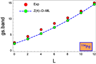
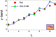
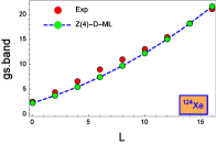
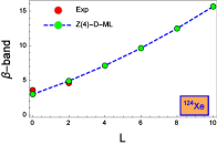
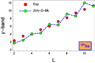
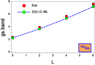
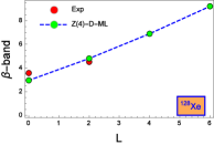
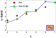
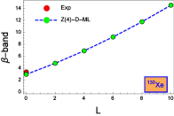
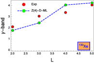
Figure 1: Comparison of the Z(4)-ML predictions for (normalized) energy levels to experimental data[32] for ^124,128,130Xe and ¹¹⁴Pd.

3 Conclusions

In this work, we have derived new solutions of the Bohr-Mottelson Hamiltonian in the triaxial $\gamma$-rigid regime within the minimal length formalism where the shape of the potential of the collective $\beta$-vibrations is assumed to be equal to an infinite square well as in the standard Z(4) model. Howeover, improved version of the Z(4) symmetry denoted Z(4)-ML is elaborated for the first time in order to describe the structural properties of some triaxial $\gamma$-rigid nuclei. Finally, through this work, one can conclude that the introduction of the minimal length concept in Z(4) allows one to enhance the numerical calculation precision of the energy spectrum of some triaxial $\gamma$ -rigid nuclei in comparison with the Z(4) model.

References

- [1] A. Bohr, Mat. Fys. Medd. Dan. Vid. Selsk. 26, 14 (1952).
- [2] A. Bohr, B. R. Mottelson, Mat. Fys. Medd. Dan. Vid. Selsk. 27,16 (1953).
- [3] D. Bonatsos, D. Lenis, E. McCutchan, D. Petrellis and I. Yigitoglu, Phys. Lett. B 649, 394 (2007).
- [4] M. Chabab, A. Lahbas and M. Oulne, Eur. Phys. J. A 51, 131 (2015).
- [5] M. Chabab, A. El Batoul, A. Lahbas and M. Oulne, Nucl. Phys. A 953, 158 (2016).
- [6] R. Budaca, P. Buganu, M. Chabab, A. Lahbas and M. Oulne, Ann. Phys. (NY) 375, 65 (2016).
- [7] M. Chabab, A. El Batoul, M. Hamzavi, A. Lahbas and M. Oulne, Eur. Phys. J. A 53, 157 (2017).
- [8] I. Yigitoglu and M. Gokbulut, Eur. Phys. J. Plus 132, 34 (2017).
- [9] D. Bonatsos, P.E. Georgoudis, N. Minkov, D. Petrellis and C. Quesne, Phys. Rev. C 88, 034316 (2013).
- [10] D. Bonatsos, P.E. Georgoudis, D. Lenis, N. Minkov and C. Quesne, Phys. Rev. C 83, 044321 (2011).
- [11] M. Chabab, A. Lahbas and M. Oulne, Phys. Rev. C 91, 064307 (2015).
- [12] M. Chabab, A. El Batoul, A. Lahbas and M. Oulne, J. Phys. G: Nucl. Part. Phys. 43,125107 (2016).
- [13] F. Iachello, Phys. Rev. Lett. 85, 3580 (2000).
- [14] F. Iachello, Phys. Rev. Lett. 87, 052502 (2001).
- [15] D. Bonatsos, D. Lenis, D. Petrellis, P. Terziev and I. Yigitoglu, Phys. Lett. B 632, 238 (2006).
- [16] R. Budaca, Phys. Lett. B 739, 56 (2014).
- [17] R. Budaca, Eur. Phys. J. A 50, 87 (2014).
- [18] M. Chabab, A. El Batoul, A. Lahbas and M. Oulne, Phys. Lett. B 758, 212 (2016).
- [19] A. S. Davydov and G. F. Filippov, Nucl. Phys. 8, 237 (1958).
- [20] A. S. Davydov and V. S. Rostovsky, Nucl. Phys. 12, 58 (1959).
- [21] N. V. Zamfir and R. F. Casten, Phys. Lett. B 260, 265 (1991).
- [22] E. A. McCutchan, D. Bonatsos, N. V. Zamfir, and R. F. Casten, Phys. Rev. C 76, 024306 (2007).
- [23] L. Fortunato, Phys. Rev. C 70, 011302 (2004).
- [24] L. Fortunato, Eur. Phys. J. A 26, 1 (2005).
- [25] L. Fortunato, S. De Baerdemacker and K. Heyde, Phys. Rev. C 74, 014310 (2006).
- [26] I. Yigitoglu and D. Bonatsos, Phys. Rev. C 83, 014303 (2011).
- [27] P. Buganu and R. Budaca, Phys. Rev. C 91, 014306 (2015).
- [28] M. Alimohammadi and H. Hassanabadi, H. Sobhani, Mod. Phys. Lett. A 31, 1650193 (2016).
- [29] M. Alimohammadi and H. Hassanabadi, Nucl. Phys. A 957, 439 (2017).
- [30] A. S. Davydov and A. A. Chaban, Nucl. Phys. 20, 499 (1960).
- [31] D. Bonatsos , D. Lenis , D. Petrellis , P.A. Terziev and I. Yigitoglu , Phys. Lett. B 621,102 (2005).
- [32] Nuclear Data Sheets (http://nndc.bnl.gov/).