High-Order Symbolic Strong-Coupling Expansion for the Bose-Hubbard Model

Abstract

Combining the process-chain method with a symbolized evaluation we work out in detail a high-order symbolic strong-coupling expansion (HSSCE) for determining the quantum phase boundaries between the Mott insulator and the superfluid phase of the Bose-Hubbard model for different fillings in hypercubic lattices of different dimensions. With a subsequent Padé approximation we achieve for the quantum phase boundaries a high accuracy, which is comparable to high-precision quantum Monte-Carlo simulations, and show that all the Mott lobes can be rescaled to a single one. As a further cross-check, we find that the HSSCE results coincide with a hopping expansion of the quantum phase boundaries, which follow from the effective potential Landau theory (EPLT).

I Introduction

In recent decades, strongly correlated systems play a crucial role in condensed matter physics. For high-temperature superconductors,sc the on-site interaction between fermions becomes more dominant than the hopping processes. Thus, considering the hopping term as a perturbation, the Hubbard model can be reduced to the $t-J$ model or the Heisenberg model at half filling. The bosonic counterpart is the Bose-Hubbard model,bh which has extensively been studied theoretically and can be realized experimentally using a gas of bosonic atoms in optical lattices.bh2 ; bh3 By reducing the tunneling processes via a deeper lattice potential or by using the Feshbach resonance technique in order to increase the interaction, those lattice systems can be tuned such that a quantum phase transition from a superfluid to a Mott insulator phase can be observed.bh2 ; bh3 But also magnetic atoms,erbium dipolar molecules,molecules or Rydberg atoms Rydberg can be loaded into an optical lattice, so that the strong long-range and anisotropic dipolar interaction plays a major role. In contrast to the weakly interacting case, strongly dipolar correlated systems exhibit many exotic phases, such as supersolid,ss1 ; ss2 ; ss3 ; triangular superradiant solid,zhang2 or other topological phases.zhang3

The Bose-Hubbard model,bh which describes the quantum phase transition between the Mott insulator to the superfluid phase, is defined by the Hamiltonian

$$\hat{H}=-t\mathop{\sum}_{\langle ij\rangle}(\hat{b}_{i}^{{\dagger}}\hat{b}_{j}+\hat{b}_{j}^{{\dagger}}\hat{b}_{i})+\mathop{\sum}_{i}\left[\frac{U}{2}\hat{n}_{i}(\hat{n}_{i}-1)-\mu\hat{n}_{i}\right],$$ (1)

where $\langle ij\rangle$ represents a sum over nearest-neighbor sites, $t$ denotes the hopping matrix element, $\hat{b}_{i}^{{\dagger}}(\hat{b}_{i})$ creates (annihilates) a particle on site $i$, $\hat{n}_{i}=\hat{b}_{i}^{{\dagger}}\hat{b}_{i}$ abbreviates the number operator, $U$ stands for the on-site repulsion, and $\mu$ is the chemical potential. The quantum phase transition was first established by using mean-field theory,bh but it is possible to obtain more accurate results by using a strong-coupling expansion (SCE) method, which was proposed by Freericks and Monien some time ago.Monien The strong-coupling ground state is given in the particle number representation, while the hopping term is treated as a perturbation, so that the energy of both the Mott insulator and a single particle (or hole) excited state can be calculated perturbatively. By equating the respective energies, the critical line between the Mott insulator and the superfluid phase can be deduced. In comparison with the mean-field approach,bh this strong-coupling expansion method shows a higher accuracy for lower spatial dimensions, especially after an extrapolation to higher orders. Therefore, SCE has been used successfully to study the Bose-glass phase in the superlattice,sc1 two-species bosons loaded into $d$-dimensional hypercubic optical lattices,sc2 ; sc2b and the supersolid-solid quantum phase transition.zhang4 In particular, the strong-coupling expansion method has turned out to be efficient for the second-order transition from an incompressible to a compressible phase. However, the calculation effort turns out to increase with the order and filling in form of a power law, so analytic expressions from SCE are usually limited up to the fourth order.

In order to obtain higher orders than the $10$th order, Eckardt et al. developed a computer assisted process-chain algorithm (PCA) eckardt ; martin based on Kato’s formulation of the perturbation calculus.kato Using the PCA, high-precision results were obtained for both the ground-state energy and the correlation function within the Mott insulator.martin Furthermore, by implementing PCA for the effective potential Landau theory (EPLT),santos ; tao2 the critical line of the quantum phase transition from the Mott insulator to the superfluid phase was determined with high precision martin ; ying so that even the corresponding critical exponents can be extracted.hinrichs In order to deal with degenerate states, such as particle-hole excitations, the PCA must be modified, as was shown by Heil and Linden for a one-dimensional (1D) system.Heil An alternative SCE approach by Elstner and Monien also obtained high-order results which can be applied to low dimensions and low filling.Elstner However, a general analytic expression for quantum phase boundaries of different fillings, orders, and dimensions is still lacking. They may help, for instance, to hint at a scaling relation between different fillings.Teichmann In addition, it is still unclear how SCE and EPLT are related although both methods deal with a perturbative hopping expansion.

In this paper, we work out a high-order symbolic SCE algorithm (HSSCE) and combine it with PCA for degenerate states in order to obtain the quantum phase boundary of the Bose-Hubbard model. To this end we briefly review in Sec. II the strong-coupling expansion, for which we propose an efficient method and list the general analytic strong-coupling series up to eighth order on chain (1D), square (2D), and cubic (3D) lattices for arbitrary filling $n$. Then the respective quantum phase boundaries are obtained in Sec. III in the thermodynamic limit by applying the Padé resummation method to the strong-coupling series and by comparing the results with those from numerical high-precision calculations. In Sec. IV, based on the analytic expression of the critical line for arbitrary filling, we rescale the Mott lobes to the infinite filling Mott lobe. Afterwards, in Sec. V, we show that the HSSCE results coincide with a hopping expansion of the high-order effective potential Landau theory (HEPLT). Finally, we draw our conclusions in Sec. VI. In addition, in order to assist writing a code, we work our algorithm in detail in Appendix A and also attach the Matlab code in the Supplemental Material.sm

II Strong-Coupling Expansion for the Bose-Hubbard Model

The strong-coupling expansion method is based on treating effects of the hopping matrix element perturbatively. It can be used to determine the second-order critical line of the incompressible phase, whose melting is caused by a proliferation of particle or hole excitations. Based on the work of Freericks and Monien,Monien one determines at first the unperturbed ground-state wave function of both the incompressible state and the particle (hole) excited state. Then one calculates the respective ground-state energies in terms of a hopping expansion by applying non-degenerate and degenerate perturbation theory, respectively. At last, by comparing the resulting ground-state energies, the corresponding critical line is deduced.

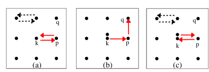
Figure 1: Second-order arrow diagrams for (a) the ground state of a Mott insulator of filling one, and also for (b) open and (c) closed arrow diagrams for the case of adding one particle. As all arrow diagrams irrelevant to site $k$, indicated by black dashed arrows, cancel each other, only the arrow diagrams relevant to site $k$, highlighted by red solid arrows, need to be considered.

Let us consider the second-order quantum phase transition of a Mott insulator as a concrete example, which is described by the Bose-Hubbard model (1). The dominant part is provided by the on-site repulsive interaction together with the chemical potential, i.e. $\hat{H}_{0}=\mathop{\sum}_{i}\left[U\hat{n}_{i}(\hat{n}_{i}-1)/2-\mu\hat{n}_{i}\right]$, whereas the perturbative part is the hopping term $\hat{H}^{\prime}=-t\mathop{\sum}_{\langle ij\rangle}(\hat{b}_{i}^{{\dagger}}\hat{b}_{j}+\hat{b}_{j}^{{\dagger}}\hat{b}_{i})$. When the tunnel matrix element $t$ vanishes, the ground state of the Mott insulator with filling $n$ is non-degenerate and uniquely given by $|\psi^{(0)}_{M}\rangle=\mathop{\prod}_{i}(\hat{b}_{i}^{{\dagger}})^{n}|0\rangle/\sqrt{n!}$. In contrast to that, the particle excited state $\hat{b}_{j}^{{\dagger}}|\psi^{(0)}_{M}\rangle$ is degenerate for $t=0$, since no matter at which site the additional particle is located, the corresponding ground-state energies coincide.

The ground-state energy of the Mott insulator reads in zeroth order of the tunnel matrix element $E^{(0)}_{M}=N[Un(n-1)/2-\mu n]$, where $N$ denotes the number of lattice sites. The first-order ground-state energy correction turns out to be zero, so the first non-vanishing correction is of second-order and follows from $E^{(2)}_{M}=\mathop{\sum}_{i\neq 0}\langle\psi^{(0)}_{M}|H^{\prime}|e_{i}\rangle\langle e_{i}|H^{\prime}|\psi^{(0)}_{M}\rangle/(E^{(0)}_{M}-E_{i})$, where $|e_{i}\rangle$ denotes an excited state with energy $E_{i}$. According to Fig. 1 (a), the second-order processes correspond to the case that each particle is hopping to the nearest neighbor site and then back. Thus, the second-order perturbation energy yields $E^{(2)}_{M}=-z(n+1)Nt^{2}/U$ where $z=2d$ stands for the coordination number of a $d$ dimensional hypercubic lattice. Then the ground-state energy of the Mott insulator up to second order in the tunnel matrix element is given by $E_{M}=E^{(0)}_{M}-z(n+1)Nt^{2}/U$.

For the particle excited state, the zeroth-order ground-state energy is given by $E^{(0)}_{p}=E^{(0)}_{M}-\mu+nU$. The general form of the ground state wave function is given by the superposition $|\psi_{p}^{(0)}\rangle=\mathop{\sum}_{j}a_{j}\hat{b}_{j}^{{\dagger}}|\psi^{(0)}_{M}\rangle$ with the normalization constraint $\mathop{\sum}_{j}|a_{j}|^{2}=1$. The first-order ground-state energy is then determined via $E^{(1)}_{p}=\langle\psi_{p}^{(0)}|\hat{H}^{\prime}|\psi_{p}^{(0)}\rangle$. In order to minimize $E^{(1)}_{p}$, we need to diagonalize the matrix $M_{i,j}=\langle\psi^{(0)}_{M}|\hat{b}_{i}\hat{H}^{\prime}\hat{b}_{j}^{{\dagger}}|\psi^{(0)}_{M}\rangle$ and take the lowest eigenvalue as the resulting first-order ground-state energy. Thus, in other words, first-order perturbation lifts the degeneracy. Based on the underlying translational symmetry of the ground state, we obtain the first-order ground-state energy $E^{(1)}_{p}=-z(n+1)t$ and the non-degenerate ground state turns out to be $|\psi_{p}^{(0)}\rangle=\mathop{\sum}_{j}\hat{b}_{j}^{{\dagger}}|\psi_{M}^{(0)}\rangle/\sqrt{Nn}$. Now we turn to second-order processes, where Fig. 1(b) and (c) depict via red solid arrow diagrams the two possible types, which occur in the presence of one additional particle. The first diagram is an open diagram, which is characterized by $|211\rangle\rightarrow|202\rangle\rightarrow|112\rangle$ with $|n_{k}n_{p}n_{q}\rangle$ denoting the occupation of the respective sites $k$, $p$, $q$ and has the corresponding energy $-(n+1)t^{2}/U$. The second one is the closed diagram $|21\rangle\rightarrow|30\rangle\rightarrow|21\rangle$ with $|n_{k}n_{p}\rangle$ representing the occupation of the sites $k$, $p$ and the related energy $-(n+2)t^{2}/(2U)$. Note that the open diagram Fig. 1(b) has the multiplicity $z(z-1)$, whereas the multiplicity of the closed one in Fig. 1(c) is given by $z$. Besides that, we have to take into account in Fig. 1(b) and (c) that there are additional $z(N-2)$ closed diagrams, indicated by black dashed arrow diagrams, which are not related to the additional particle. Thus, the second-order ground-state energy results in $E_{p}^{(2)}=-[z(N-2)(n+1)+z(n+2)/2+z(z-1)(n+1)]t^{2}/U$ and the total energy of the particle excited state is given by $E_{p}=E^{(0)}_{M}-\mu+nU-z(n+1)t+E_{p}^{(2)}$. Finally, equating the Mott and the particle excited ground-state energy according to $E_{M}=E_{p}$, we get the following critical line up to second order in the tunnel matrix element $t$: $\mu_{p}=nU-z(n+1)t-[z(n+2)/2+z(z-1)(n+1)-2z(n+1)]t^{2}/U$.

However, the number of arrow diagrams is of the order of the lattice size $N$, so this calculation is not practical in the thermodynamic limit even with the process-chain approach. Therefore, we introduce here a novel strong-coupling method, which turns out to be more practical and efficient as it is quite suitable for a computer implementation. From the above derivation of the second-order result for the critical line, we read off that perturbative calculations follow more easily from neglecting all energy contributions, which are not related to the site $k$, where the additional particle is located, as all those contributions irrelevant to site $k$ in $E_{M}$ and $E_{p}$ cancel each other at the end. Thus, in order to obtain the critical line to higher orders in the tunnel matrix element most efficiently, we need to consider the following three steps:
(i) We calculate the energies of the diagrams related to the site $k$ based on the ground state $|\psi^{(0)}_{M}\rangle$, and name them energy corrections. To this end we only need to find all closed arrow diagrams related to site $k$ and calculate the contribution for each diagram to the non-degenerate ground-state energy. In Fig. 1 (a), we have $z$ hopping processes, where a particle at site $k$ hops to a nearest neighbor site and then back, as well as $z$ hopping processes, where a particle at a neighbor site hops to site $k$ and back, thus the second-order energy correction results is $-2z(n+1)t^{2}/U$.
(ii) We only determine the energy, which is related to the additional particle, and name it strong-coupling (SC) energy. To this end we need to find all arrow diagrams related to site $k$ and calculate the contribution of each diagram to the degenerate ground-state energy. In Fig. 1, the diagrams (b) and (c) have the multiplicity $z$ and $z(z-1)$, respectively, thus the corresponding SC energies read $-z(n+2)t^{2}/(2U)$ and $-z(z-1)(n+1)t^{2}/U$.
(iii) Equating the energy of processes (i) and (ii), we obtain the resulting SCE critical line.
Based on this strong-coupling expansion method, we only need to consider a finite number of diagrams, combine their evaluation with the process-chain method, and then obtain their perturbative value. Note that for the case of the hole excitation, the calculations proceed similarly, except that the arrows point then in the direction, where the hole moves.

In order to implement this method, we used an algorithm proposed by Heil and Linden,Heil but in our case each step is realized in terms of a symbolic calculation. Then, the representation of the coefficients in each order is an analytic function of both the filling $n$ and the hopping amplitude $t$. In order to make the implementation of the algorithm more explicit, we explain the details in Appendix A, and make the corresponding Matlab code available in the Supplemental Material.sm With this we have determined the critical lines of the quantum phase diagram of the Bose-Hubbard model for a general Mott lobe $n$, which were obtained with symbolic calculations up to the 8th order. The strong-coupling results for both the upper and the lower critical line of the Mott insulator with respect to both particle and hole excitations are defined according to

$$\frac{\mu_{\rm p}}{U}=1-\mathop{\sum}_{i=1}^{\infty}\beta_{\rm u}^{(i)}\left(\frac{t}{U}\right)^{i}$$ (2)

and

$$\frac{\mu_{\rm h}}{U}=\mathop{\sum}_{i=1}^{\infty}\beta_{\rm d}^{(i)}\left(\frac{t}{U}\right)^{i}\,,$$ (3)

respectively. The analytic expressions with coefficients up to 8th order are given in Appendix B.

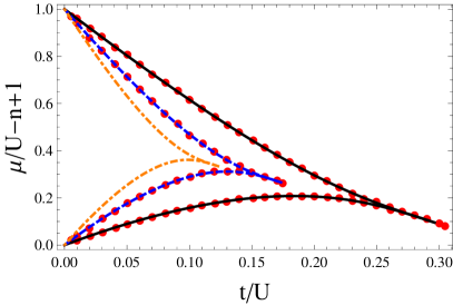
Figure 2: Quantum phase diagrams of Bose-Hubbard chain for filling $n=1$ (black solid line), $n=2$ (blue dashed line), and $n=3$ (orange dot-dashed line). The red dots are DMRG results for filling $n=1$ and $n=2$.Gebhard

III Quantum Phase diagram for Bose-Hubbard model

In order to reconstruct from such perturbative results the whole quantum phase diagram in the thermodynamic limit, we need to know the scaling behaviour of the quantum phase transition. According to previous works,bh ; Sachdev the Mott-superfluid quantum phase transition of the Bose-Hubbard model with dimension $d\geq 2$ belongs to the $d+1$ dimensional $XY$ universality class. But in one dimension the quantum phase transition turns out to be of the Berezinsky-Kosterlitz-Thouless (BKT) type, which has to be treated separately.

III.1 BKT Universality Class

In the one-dimensional case the quantum phase boundary can be rewritten as $\mu_{p(h)}=B(t)\pm\Delta(t)/2$, where the strong-coupling series for both the mean energy $B(t)=(\mu_{p}+\mu_{h})/2$ and the energy gap $\Delta(t)=\mu_{p}-\mu_{h}$ follow from from Eqs. (21) and (22), respectively. On the other hand we know for the universality class of Berezinsky-Kosterlitz-Thouless that the energy gap $\Delta(t)$ is characterized by a non-analytic behaviour slightly below the critical point $t_{c}$ according to Monien ; Monien2

$$\Delta(t)=A\exp\left(-\frac{W}{\sqrt{t_{c}-t}}\right)\,,$$ (4)

with some coefficients $A$ and $W$, so we conclude $[\log\Delta(t)]^{2}\propto(t_{c}-t)^{-1}$. Such a divergent behaviour could be recovered from the strong-coupling series of $[\log\Delta(t)]^{2}$, which is available in terms of Eqs. (21) and (22) in Appendix B. up to the $8$th order by applying the Padé resummation method padebook

$$[\log\Delta(t)]^{2}=\frac{{\displaystyle\sum_{m=0}^{m_{\rm max}}}a_{m}t^{m}}{1+{\displaystyle\sum_{n=1}^{n_{\rm max}}}b_{n}t^{n}}\,.$$ (5)

To this end the corresponding Taylor series of the left- and right-hand side of Eq. (5) are used to obtain the respective coefficients $a_{m}$ and $b_{n}$ from fitting with the restriction $n_{\rm max}+m_{\rm max}=8$. The most natural way to achieve this is to choose $n_{\rm max}=m_{\rm max}=4$. Note that we also have to adopt a Padé resummation similar to Eq. (5) for the strong-coupling series of the mean energy $B(t)$ in order to describe the re-entrance behaviour of the Mott lobe, which is typical for a phase transition of the Berezinsky-Kosterlitz-Thouless type. In this way we determine the whole quantum phase diagram for different fillings $n$.

	HSSCE		numerical
	$t_{c}/U$	$\mu_{c}/U$	$t_{c}/U$
	$d=1$
$n=1$	$0.296$	$0.0956$	$0.30(1)$
$n=2$	$0.173$	$1.2659$	$0.175(2)$
$n=3$	$0.123$	$2.3339$
	$d=2$
$n=1$	0.05989	0.3705	0.05974(3)
$n=2$	0.03530	1.4238
$n=3$	0.02509	2.4459
	$d=3$
$n=1$	0.03415	0.3929	0.03408(2)
$n=2$	0.02013	1.4369
$n=3$	0.01431	2.4552

Table 1: Critical hopping amplitude and chemical potential at the lobe tip for different dimensions $d$ and filling numbers $n$. The HSSCE results are determined in combination with an $8$th order Padé resummation. The $1d$ numerical result stems from DMRG calculations,Gebhard ; Kollath ; Polkovnikov while those for $2d$ and $3d$ are obtained from QMC simulations.sv1 ; sv2

As shown in Fig. 2, a quantitative comparison with DMRG calculations Gebhard at low filling $n$ demonstrates that the quantum phase boundaries determined from HSSCE together with a Padé resummation reveal a high accuracy except from tiny deviations at the lobe tip. In particular, the critical hopping amplitude $t_{c}$ coincides in our method with a real, positive simple pole of Eq. (5), which turns out to be unique. Table 1 lists the critical hopping amplitude $t_{c}$ for the first three fillings $n$. Our results combined with various DMRG calculations have established the consensus that $t_{c}/U\approx 0.3$ for $n=1$. But note that the results of DMRG calculations for the critical point $t_{c}$ have also relatively large uncertainties and slightly deviate depending on the chosen observables since the gap becomes so small and requires extremely large system sizes. For filling $n=1$, initial estimates were given to be $t_{c}/U=0.277\pm 0.01$ Monien2 and have now been improved to $t_{c}/U=0.3050\pm 0.001$ from density density correlations Gebhard (the red dot shown in Fig. 2), $t_{c}/U=0.2980\pm 0.005$ from the von-Neumann entropy,Kollath and $t_{c}/U=0.3030\pm 0.009$ from the energy gap.Polkovnikov In addition, for increasing fillings $n$, we observe that the re-entrance behaviour weakens and tends to disappear. This result is an immediate consequence of the particle-hole symmetry which is recovered in the limit of infinite filling $n\rightarrow\infty$ irrespective of the spatial dimension. Indeed, the Hamiltonian (1) does not change with the transformation $\hat{b}^{{\dagger}}\rightarrow\hat{b}^{\prime}$, $\hat{b}\rightarrow\hat{b}^{\prime{\dagger}}$, which implies for the filling $n\rightarrow n^{\prime}+1\approx n^{\prime}$. This is reflected in the strong-coupling results for the quantum phase boundaries listed in Appendix B by the property that the coefficients of the highest filling in the upper and the lower branch have the same absolute value but a different sign.

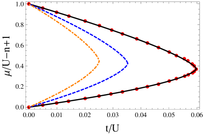
Figure 3: Quantum phase diagram of $2$d bosonic lattice system for $n=1$ (black solid line), $n=2$ (blue dashed line), and $n=3$ (orange dot-dashed line). For $n=1$ we also show QMC simulation results (red dot).sv2

III.2 XY Universality Class

For higher dimensional systems $d\geq 2$, the energy gap follows slightly below the critical point $t_{c}$ the scaling law $\Delta(t)=A(t)(t_{c}-t)^{z\nu}$.bh ; Sachdev Here $A(t)$ represents a regular function, whereas $z$ and $\nu$ denote critical exponents, which characterize the dynamics and the correlation function of the respective universality class.Zinn-Justin ; Kleinert Thus, also $\partial(\log\Delta(t))/\partial t$ has a simple pole at $t_{c}$, which can be determined via the Padé resummation method. The resulting quantum phase diagram for different fillings $n$ for the dimensions $d=2$ and $d=3$ are shown in Figs. 3 and 4, respectively. We conclude that the analytically obtained quantum phase boundaries match quite well with QMC simulation result at filling $n=1$ in both two and three dimensions. The real, positive simple pole of the Padé resummation, which turns out again to be unique, provides the critical points $t_{c}$ for different filling numbers $n$, where the lowest three values are listed in Table 1. Moreover, the corresponding residue yields a value for the critical exponent $z\nu$ listed in Table 2. Our results reveal that $z\nu$ slightly depends on the filling number $n$, but still deviates from the critical exponent of XY models.xy Thus, higher order terms may need to be considered in a future work, in order to diminish that deviation.

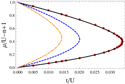
Figure 4: Quantum phase diagram of $3$d bosonic lattice system for $n=1$ (black solid line), $n=2$ (blue dashed line), and $n=3$ (orange dot-dashed line). For $n=1$ we also show QMC simulation results (red dots).sv1

	$n=1$	$n=2$	$n=3$	$n\rightarrow\infty$	XY
$d=2$	$0.6965$	$0.6951$	$0.6948$	$0.6945$	$0.6715$ xy
$d=3$	$0.5625$	$0.5647$	$0.5656$	$0.5663$	$0.5$

Table 2: Critical exponents $z\nu$ of Mott-superfluid phase transitions in two and three dimensions.

IV Rescaling Properties of different filling

In this section we investigate systematically the filling-dependent rescaling properties of the Bose-Hubbard quantum phase diagram and restrict ourselves to the case of $2$d and the $3$d. At first, we consider for different fillings $n$ the rescaling properties of the critical point $t_{c}(n)$, which represents the tip of the Mott lobe. To this end we follow Ref. [Teichmann, ] and use its second-order strong-coupling result in order to re-express the hopping amplitude of the lobe tip for large filling $n$ according to

$$\frac{t_{c}(d,n)}{U} = \frac{2d-\sqrt{-10d+12d^{2}}}{(10-8d)d}$$ (6)

$$\times\left[1-\frac{1}{2n}+O\left(\frac{1}{n^{2}}\right)\right]\,\frac{1}{n}\,.$$

Thus, in the limit of large filling, the effects of dimension $d$ and filling $n$ turn out to decouple. Assuming that such a decoupling property also holds for higher strong-coupling orders, we perform for the critical hopping amplitude the generic ansatz

$$\frac{t_{c}(d,n)}{U}=f_{t}(d)\,\frac{g_{t}(n)}{n}\,,$$ (7)

where the filling-dependent factor represents a Taylor series in $1/n$:

$$g_{t}(n)=1+\sum_{i=1}^{\infty}\frac{a_{i}}{n^{i}}\,.$$ (8)

In the limit of infinite filling we then conclude

$$f_{t}(d)=\lim_{n\rightarrow\infty}n\frac{t_{c}(d,n)}{U}\,.$$ (9)

This means that $f_{t}(d)$ can be calculated both for $d=2$ and $d=3$ from the term with highest filling number $n$ in each strong-coupling order for both the upper and the lower quantum phase boundary presented in Appendix B. Note that, due to the particle-hole symmetry mentioned above, the coefficients of the highest filling in the upper and the lower branch have the same absolute value but a different sign.

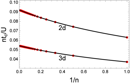
Figure 5: Critical hopping amplitudes $t_{c}$ for filling numbers $n$ from $1$ to $100$ (red dots) compared with the value of $f_{t}(d)$ times the rescaling function $g_{t}(n)$ (black line) in two and three dimensions.

After having obtained $f_{t}(d)$ for $d=2$ and $d=3$, we directly read off from Eq. (7) in each strong-coupling order the function $g_{t}(n)=nt_{c}(d,n)/[f_{t}(d)U]$ as a Taylor series in $1/n$. In order to approach the infinite-order case, we perform a Padé resummation and rewrite the filling-dependent function as

$$g_{t}(n)\approx\tilde{g}_{t}(n)=\frac{1+{\displaystyle\sum_{i=1}^{M}\frac{\alpha_{i}}{n^{i}}}}{1+{\displaystyle\sum_{j=1}^{M}\frac{\beta_{j}}{n^{j}}}}\,.$$ (10)

Here $M$ is an integer, which characterizes the order of the Padé resummation. The resulting function $\tilde{g}_{t}(n)$ represents the rescaling function of the critical hopping amplitude. In Fig. 5 we have chosen $M=4$ and have used the critical hopping amplitude at the tip of the first 100 Mott lobes to fit the scaling function. In addition it turns out that the rescaling functions in two and three dimensions nearly coincide, which supports a posteriori the above assumption from Eq. (7) that dimension $d$ and filling $n$ decouple.

Furthermore, one can also use a similar strategy in order to investigate the rescaling properties of the critical chemical potential $\mu_{c}(d,n)/U$ at the lobe tip. But then the above mentioned particle-hole symmetry for infinite filling implies for the chemical $\lim_{n\rightarrow\infty}\mu_{p}/U=1-\lim_{n\rightarrow\infty}\mu_{h}/U$, so the critical chemical potential reads $\lim_{n\rightarrow\infty}\mu_{c}/U=1-\lim_{n\rightarrow\infty}\mu_{c}/U=1/2$. Thus, the dimension dependent function is then given by $f_{\mu}(d)=\lim_{n\rightarrow\infty}\mu_{c}/U=1/2$, so the rescaling function $g_{\mu}(d,n)=2\mu^{\prime}_{c}(d,n)/U$ with $\mu_{c}^{\prime}(d,n)/U=\mu_{c}(d,n)/U-n+1$ results as a Taylor series in $1/n$, for which we perform a Padé resummation

$$g_{\mu}(d,n)\approx\tilde{g}_{\mu}(d,n)=\frac{1+{\displaystyle\sum_{i=1}^{M}\frac{\alpha^{\prime}_{i}}{n^{i}}}}{1+{\displaystyle\sum_{j=1}^{M}\frac{\beta^{\prime}_{j}}{n^{j}}}}\,.$$ (11)

Note that, in contrast to the critical hopping, the rescaling function $\tilde{g}_{\mu}(d,n)$ for the chemical potential turns out to have a residual dependence on the dimension $d$.

By assuming that the entire critical lines have the same rescaling functions at the tips of the Mott lobes, we can map all Mott lobes for different filling numbers to the infinite filling lobe as follows. For each critical point $\{\mu^{\prime}(d,n)/U,nt(d,n)/U\}$ in the lower branch of the Mott lobe, we define the rescaled value as $\{\mu^{\prime}_{\infty}/U,(tn)_{\infty}/U\}=\{\mu^{\prime}(d,n)/[\tilde{g}_{\mu}(n)U],t(d,n)n/[\tilde{g}_{t}(n)U]\}$ and, correspondingly, for each critical point in the upper branch we rescale according to $\{\mu^{\prime}_{\infty},(tn)_{\infty}/U\}=\{1-[1-\mu^{\prime}(d,n)/U]/[2-\tilde{g}_{\mu}(n)],t(d,n)n/[\tilde{g}_{t}(n)U]\}$. In Fig. 6 we observe that all scaled Mott lobes, obtained from different filling numbers $n$, deviate only slightly from the quantum phase boundary at infinite filling.

Finally, we comment upon why the rescaling property turns out to be more complicated for the one-dimensional system. Although we could also find a rescaling function for the critical point, this rescaling function could not be used to map all the lobes to the infinite filling lobe. Whereas a Mott lobe with finite filling reveals a re-entrance phenomenon due to the BKT quantum phase transition, this re-entrance phenomenon disappears in the limit of an infinite filling due to the particle-hole symmetry between the upper and the lower phase boundary. Thus, in one dimension there does not exist a universal rescaling function for all points of the quantum phase diagram.

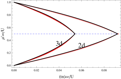
Figure 6: Scaled Mott lobe obtained from different fillings $n$ (red dots) compared with infinite filling quantum phase diagram (black line). For both dimensions $d=2$ and $d=3$ the scaled Mott lobes deduced from filling number $n=1,2,3,4,10,100,10000$ are almost on top of each other.

V Relation with high-order effective potential landau theory

As has already been explained in the introduction, both SCE Monien and EPLT santos ; tao2 represent two analytical perturbative methods for determining the quantum phase boundary of lattice systems. Usually the accuracy of their results are only compared in lower orders. Thus, in order to allow for a comparison in higher orders, we have also investigated the $2$d Bose-Hubbard model with the HEPLT method from Ref. [martin, ] up to the $10$th order. Whereas the HSSCE method allows to determine the upper or the lower quantum phase boundary with one single calculation, HEPLT is more involved and needs independent calculations to obtain the critical hopping for each chemical potential. Note that, up to the same order, HSSCE turns out to be faster than HEPLT because it has not to deal with additional source terms.

Comparing the accuracy of both methods for $d=2$ in $10$th order, we find that the effective potential result has an error of about $2.4\%$, while the strong-coupling result turns out to have an error of about $5.0\%$. Thus we conclude that HEPLT is more accurate than HSSCE up to the same order. From Fig. 7 we also read off that the HEPLT result always gives smaller hopping values than the QMC result, while the HSSCE result gives larger values. Thus, we could use both methods in order to determine the region in the quantum phase diagram, where the phase boundary must exist. Extrapolating the results for both methods to infinite order yields quantum phase boundaries, which are basically indistinguishable from QMC sv2 in the $2$d system. However in $3$d a comparison with results from QMC sv1 reveals that extrapolating the $10$th order of HSSCE has the same accuracy as extrapolating the $8$th order of HEPLT.martin Thus, up to the same order, the HEPLT method turns out to be more accurate in higher dimensional systems.

In a previous paper tao1 we have pointed out the intriguing observation that, up to the second order, the SC coefficients coincide with those of a hopping expansion of the EPLT quantum phase boundary. Thus, for the Mott lobe $n$, one obtains the SC upper (lower) critical line by performing a hopping expansion of the EPLT quantum phase boundary around $\mu/U=n-1$ ($\mu/U=n)$. In view of proving such relations also for higher orders, we perform a symbolic calculation for the HEPLT method up to the $8$th order. By a corresponding hopping expansion of the HEPLT quantum phase boundary we obtain, indeed, the same coefficients of both the upper and the lower HSSCE critical lines. As shown in Fig. 7, the QMC results are located between the HSSCE and the HEPLT critical lines, so both methods can be considered as an overestimation and an underestimation, respectively. We think the reason is that, HSSCE neglects high order corrections but HEPLT includes more.

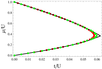
Figure 7: Comparison of quantum phase diagrams for $d=2$ via HSSCE (black line) and HEPLT (red dots)martin in $10$th order with QMC results (green dots)sv2 at $n=1$.

VI conclusion

In this paper we developed a symbolic implementation the process-chain approach eckardt ; martin for applying the strong-coupling expansion method Monien to very high orders. The resulting analytic symbolic expressions allow a detailed analysis of how the critical lines depend on the fillings numbers and the dimensions. As a concrete example we have calculated for the Bose-Hubbard model the quantum phase diagram between the superfluid and the Mott insulator in different dimensions. Applying the Padé resummation method, we have obtained the critical lines in the thermodynamic limit for arbitrary fillings. A comparison with DMRG and QMC calculations the phase transition at filling $n=1$ demonstrates that the HSSCE method is quite accurate, so that it can be also used reliably determine the transition lobes at higher fillings which are hard to obtain from recent numerical and analytic methods.

In addition, the analytic expression of the phase boundaries can help to investigate systematically the rescaling properties of the quantum phase diagram. At the lobe tips we have found that the rescaling functions of the critical hopping almost coincide for both two and three dimensions, while the corresponding rescaling functions of the critical chemical potential turn out to be different. With this rescaling at the lobe tip it has then been possible to approximately map all the Mott lobes of different fillings to the infinite filling Mott lobe.

Finally, we have compared the HEPLT with the HSSCE method developed here and have concluded that the latter is easier to implement. However, it has also turned out that HSSCE is less accurate as HEPLT up to the same order. Furthermore, we have verified an intimate relation been both methods. Namely, the quantum phase boundaries from HEPLT and HSSCE have turned out to agree up to the $8$th order in a power series with respect to the hopping.

In addition, we present our algorithm in greater detail in Appendix A, so that the respective steps should be reproducible for the reader. Further information is accessible in a Matlab code in the Supplemental Material, which can be downloaded from our homepage.sm

We conclude that our paper works out in detail a general symbolic high-order perturbation theory, whose applicability is not limited to the Bose-Hubbard model. Instead it may also be suitable to analyze other lattice systems, which describe, for instance, the supersolid-solid transition,ss1 a mixture of two bosonic species,sc2 ; sc2b three-body interactions,zhang4 and even frustrated systems like Kagome superlattices kagomelattice suffering from the sign problem. Furthermore it should be noted that our theoretical high-precision results could, in principle, be checked with in situ density measurements density and single atom detection singleatom as they are possible these days, for instance, with the quantum gas microscope microscope or the scanning electron microscope.electron

Appendix A: Algorithm of high-order strong-coupling expansion

When a strong-coupling perturbation theory is used to determine the ground-state energy of a Bose-Hubbard model, the respective orders can be calculated recursively. To this end one has to consider different types of hopping processes which contribute to the considered perturbative order of the ground-state energy. However, such an algorithm has two disadvantages. (a) High-order results are based on lower orders. (b) It is hard to automatically generate the relevant hopping processes. In order to overcome those problems, Eckardt suggested to use the Kato representation of perturbation theory.eckardt This allows to produce the respective perturbative terms in each order via a process chain approach which generates and evaluates the respective diagrams systematically. In view of the high-order strong-coupling expansion, we also use similar strategies. In the following, we discuss the three parts how to implement the algorithm in detail and take the lower-order terms for the Bose-Hubbard model in a square lattice as illustrative examples.

A.1 Kato representation

Kato worked out a particular representation for the perturbative terms of perturbation theory.kato Therein, the $n$th order contribution to the ground-state energy for a perturbation of the Hamiltonian $H^{\prime}$ is given by the trace

$$E^{(m)}={\rm Tr}\sum_{\{\alpha_{\ell}\}}S^{\alpha_{1}}H^{\prime}S^{\alpha_{2}}H^{\prime}...H^{\prime}S^{\alpha_{m+1}}\,.$$ (12)

Here each term is characterized by a Kato trace list

$$\langle\alpha_{1}\alpha_{2}...\alpha_{m+1}\rangle\,,$$ (13)

where the integers $\alpha_{1},\ldots,\alpha_{m+1}$ fulfill the condition

$$\sum_{\ell=1}^{m+1}\alpha_{\ell}=m-1,\hskip 14.22636pt\alpha_{\ell}\geq 0\,.$$ (14)

Furthermore, the operators $S^{\alpha_{\ell}}$ are defined via

$$S^{\alpha_{\ell}}=\begin{cases}-|g\rangle\langle g|&\mbox{if $\alpha_{\ell}=0$}\\ \frac{|e\rangle\langle e|}{\left(E_{g}^{0}-E_{e}^{0}\right)^{\alpha_{\ell}}}&\mbox{if $\alpha_{\ell}\neq 0$}\,,\end{cases}$$ (15)

where $|g\rangle,|e\rangle$ and $E_{g}^{0},E_{e}^{0}$ denote wave functions and energies of the ground state and the excited states, respectively. Thus, we read off from Eq. (15) the relation

$$S^{\alpha_{i}}S^{\alpha_{j}}=\begin{cases}-S^{0}&\mbox{$\alpha_{i}=\alpha_{j}=0$}\\ 0&\mbox{$\alpha_{i}=0,\alpha_{j}\neq 0$ or $\alpha_{i}\neq 0,\alpha_{j}=0$}\\ S^{\alpha_{i}+\alpha_{j}}&\mbox{$\alpha_{i}\neq 0,\alpha_{j}\neq 0$}\end{cases}$$ (16)

which is useful for simplifying products of operators $S^{\alpha_{\ell}}$. Additionally, we can conclude from Eq. (14) that there are at least two numbers in the Kato trace list $\langle\alpha_{1}\alpha_{2}...\alpha_{m+1}\rangle$ which are zero. The goal is to use Eq. (16) and the cyclic permutation of operators under the trace to move the $S^{0}$-operators to the outside of the trace, so the expression can be rewritten in general as

$$\langle g|H^{\prime}S^{\alpha_{1}^{\prime}}H^{\prime}...S^{\alpha_{m-1}^{\prime}}H^{\prime}|g\rangle.$$ (17)

If $\alpha_{1}=\alpha_{m+1}=0$ we immediately obtain the new indices $\alpha_{j}^{\prime}=\alpha_{j+1}$. If $\alpha_{1}\neq\alpha_{m+1}=0$ or $\alpha_{1}\neq\alpha_{m+1}=0$ the expression vanishes according to Eq. (16), so this case does not need to be considered. Finally, if $\alpha_{1}\neq 0$ and $\alpha_{m+1}\neq 0$ cyclic permutations are used until $S^{0}=-S^{0}S^{0}$ appears first in the product under the trace, which can then again be written in the form of Eq. (17) with a negative sign and one of the new indices with value $\alpha_{1}+\alpha_{m+1}$. We define the resulting reduced list of indices as a Kato-list and use the abbreviated representation

$$\left(\alpha_{1}^{\prime}\alpha_{2}^{\prime}...\alpha_{m-1}^{\prime}\right).$$ (18)

So far two ways have been used to calculate the Kato-lists. One was suggested by Eckardt eckardt and can be realized by the following steps. At first we substitute the operator $S^{0}$ with $-|g\rangle\langle g|$ into the Kato-list and use the abbreviation $|g\rangle\rightarrow)$ and $\langle g|\rightarrow($. With this the Kato-list changes into an array of elementary matrix element (EME) denoted by $(.....)$, in which the operator $S^{0}$ no longer exists. Note that the EME has the reflection symmetry, so we have, for instance, $(\alpha_{1}\alpha_{2}\alpha_{3})=(\alpha_{3}\alpha_{2}\alpha_{1})$. For convenience reasons we always change the form of the EME such that we take the smaller one, e.g. we use $(121321)$ and not $(123121)$. After that, to order the array of EMEs, we define the relative value of the EME with the following two rules. (i) The numbers $\alpha$ of the operators $S^{\alpha}$ in the EME are firstly compared, thus we have $(111)>(12)$. (ii) When the numbers coincide, then we compare the integer $\alpha$ of the first non-equal operator $S^{\alpha}$, so we have $(123)<(132)$. Along these lines we can order the EMEs in the Kato-list. Consider, for instance, $\langle 20210{\bf 1}1001\rangle$ as an example for a Kato trace list, which can be transformed into the Kato-list $-({\bf 1}1003021)$.eckardt The resulting EMEs $(11)()(3)(21)$ can then be ordered to obtain $()(3)(11)(12)$, which is stored as a Kato-list $-(03011012)$. At the end, the final Kato-lists can be ordered according to similar rules as the array of EMEs.

Let us take the fourth-order perturbative term as a concrete example to show how to generate the Kato-lists step by step and how to order them for later usage. It can be proved that the resulting fourth-order Kato representation coincides with the standard result of perturbation theory.

Algorithm		Output
1. Generate all Kato trace lists for the considered order $n=4$.		$\langle 30000\rangle$,$\langle 21000\rangle$,$\langle 20100\rangle$,…,$\langle 10101\rangle$,…,$\langle 00003\rangle$
2. Neglect all terms which have a zero at one end and are non-zero at the other end due to the second line of Eq. (16).		$\langle 03000\rangle$,$\langle 02100\rangle$,$\langle 02010\rangle$,$\langle 00210\rangle$,$\langle 01110\rangle$,$\langle 00120\rangle$, $\langle 01020\rangle$,$\langle 01200\rangle$,$\langle 00030\rangle$,$\langle 10011\rangle$,$\langle 10101\rangle$,$\langle 11001\rangle$, $\langle 20001\rangle$,$\langle 10002\rangle$,$\langle 00300\rangle$
3. Change Kato trace list to Kato-list.		$(300)$,$(210)$,$(201)$,$(021)$,$(111)$,$(012)$,$(102)$,$(120)$, $(003)$,$-(012)$,$-(102)$, $-(210)$,$-(300)$,$-(300)$,$(030)$
4. Perform the substitutions $|g\rangle\rightarrow)$ and $\langle g|\rightarrow($ and order array of EMEs.		$()()(3)$,$-()(12)$,$-(1)(2)$,$-()(12)$,$(111)$,$-()(12)$,$-(1)(2)$,$-()(12)$, $()()(3)$,$()(12)$,$(1)(2)$,$()(12)$,$-()()(3)$,$-()()(3)$,$()()(3)$
5. Collect same arrays and determine their weight.		$-(1)(2)$,$-2()(12)$,$()()(3)$,$(111)$
6. Order and change them back to Kato-list.		$(003)$,$2(012)$,$(102)$,$(111)$

The advantage of this algorithm is that one can get for each order the smallest number of Kato-lists, so that the computation time is drastically reduced. But the Kato-lists following from the above algorithm are only suitable provided that the ground state is non-degenerate. Let us illustrate this by the process $\langle g_{1}|H^{\prime}S^{\alpha_{1}^{\prime}}H^{\prime}|g_{2}\rangle\langle g_{2}|H^{\prime}S^{\alpha_{2}^{\prime}}H^{\prime}|g_{3}\rangle$, which involves the three degenerate ground states $|g_{1}\rangle,|g_{2}\rangle,|g_{3}\rangle$ and can be represented by the Kato-list $(\alpha_{1}^{\prime}0\alpha_{2}^{\prime})$. If we transform the Kato-list into EMEs and change their order, the calculation process may be changed to $\langle g_{2}|H^{\prime}S^{\alpha_{1}^{\prime}}H^{\prime}|g_{3}\rangle\langle g_{1}|H^{\prime}S^{\alpha_{2}^{\prime}}H^{\prime}|g_{2}\rangle$. But this cannot be mapped back to the Kato-list $(\alpha_{2}^{\prime}0\alpha_{1}^{\prime})$ as the number $0$ in the Kato-list corresponds to $\sum_{j}|g_{j}\rangle\langle g_{j}|$, but not $\sum_{i,j}|g_{i}\rangle\langle g_{j}|$.

A second approach for calculating Kato-lists was proposed in Ref. [Heil, ] in order to also treat degenerate ground states, which was then applied to a 1D system. Here the Kato-lists (18) have to fulfill the conditions

$$\mathop{\sum}_{\ell=1}^{m-1}\alpha_{\ell}^{\prime}=m-1,\hskip 14.22636pt\alpha_{\ell}^{\prime}\geq 0$$ (19)

and

$$\sum_{\ell=1}^{s}\alpha_{\ell}^{\prime}\leq s,\hskip 14.22636pt\mbox{for $s=1,...,m-2$}\,.$$ (20)

Thus, more Kato-lists appear in each order, so the computational effort increases. In particular, now each Kato-list appears with the multiplicity one. For instance, in fourth order we no longer have the Kato-lists $(003)$,$2(012)$,$(102)$,$(111)$ for a non-degenerate ground state but instead $(003),(012),(021),(102),(111)$.

It should be remarked that in the algorithm the generated Kato-lists will be stored in binary form using a suitable hashing technique, so that it is efficient to search for matching Kato-lists, which will be useful for the calculation below.

In conclusion, the original Kato-lists in Ref. [eckardt, ] are useful for calculating non-degenerate ground-state energies as they show up, for instance, for Mott states. In contrast to this, the degenerate states of particle and hole excitations, as they appear within the strong-coupling method, have to be determined from Kato-lists of multiplicity one by taking into account the restrictions in Eqs. (19) and (20).Heil

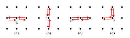
Figure 8: Arrow diagrams of 4th order in the square lattice, which are topologically equivalent

A.2 Arrow diagrams generalization

Whereas the determination of the underlying Kato-lists is independent of the considered system, we now turn to their diagrammatic representation, which does depend on the underlying Hamiltonian or the topology of the lattice. To this end we follow Refs. eckardt ; Heil and remark that an expression $\langle e_{1}|H^{\prime}|e_{2}\rangle$ in the Kato-list corresponds to a hopping process on the lattice, which can be represented by an arrow. Thus, in a lattice system, each perturbative term can be graphically depicted as an arrow diagram. According to the linked cluster theorem, only connected diagrams contribute to the ground-state energy, thus we only need all non-equivalent connected arrow diagrams. Whereas for the calculation of the non-degenerate ground-state energy only closed connected diagrams appear, for degenerate ground-state energies also open connected diagrams have to be considered. For instance, for a particle (hole) excited degenerate ground state, each perturbative term is equivalent to the hopping of a particle (hole) to another site, so any open connected diagram has exactly two ends. Thus, the respective arrow diagram can be interpreted as the path of a moving particle.

In order to generate all non-equivalent arrow diagrams, we fix at first the starting point at the center, and use different numbers or characters to label the respective directions. For instance, in case of a square lattice, we abbreviate up as ‘$u$’, down as ‘$d$’, left as ‘$l$’, and right as ‘$r$’. After that, we get all possible connected arrow diagrams by applying combinatorics and represent them with the corresponding arrays of characters. Let us consider the second-order arrow diagrams as a concrete example: in case of a square lattice we have in total $16$ diagrams, but only $(ud)$, $(du)$, $(lr)$, and $(rl)$ represent closed diagrams, whereas the others are open ones. Each diagram can have a non-unique representation, such as the 4th-order diagram in Fig. 8(a), which can be represented by $(lrrl)$ or by $(rllr)$. But if we define the priority $r<u<l<d$ and only take the smallest one according to this order, the array corresponding to Fig. 8(a) is identified with $(rllr)$. Proceeding in this way we avoid an overcounting of diagrams.

However, judging whether the diagram representation is the smallest one is not trivial, since there are several ways to follow a given set of arrows that point in and out from a central site as shown in Fig. 9. All possible paths can be drawn in form of a tree graph as shown in the right panel of Fig. 9. The smallest path, which passes through all the arrows, is the one to be determined. To this end, one can go through the whole diagram by moving in each step through the smallest arrow, but it is not allowed to move through one and the same arrow again. If one cannot finish with passing all the arrows, one has to trace back to the latest site, which has at least two arrows pointing out, and has now to choose the next smallest arrow to move through. After several tracing back processes, one gets the smallest diagram representation, when all arrows are passed.

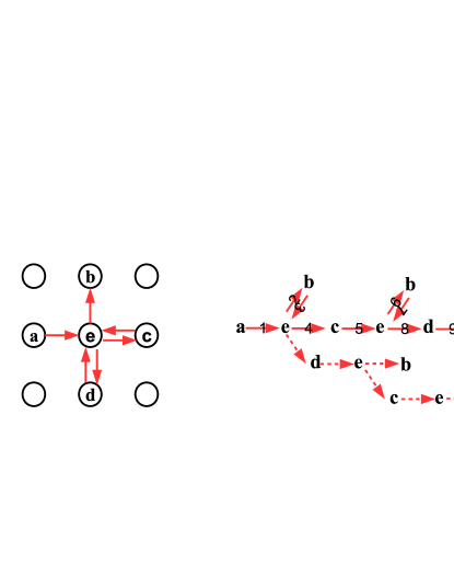
Figure 9: One $6$th-order arrow diagram labeled with $(rdurlu)$ is shown in the left panel, its corresponding tree graph is shown in the right panel. Red solid arrows in the right panel are paths, which are passed due to the algorithm, and the dashed arrows represent other possible paths. The arrows $(2,3,6,7)$ indicate trace back process, so the smallest path is $(1,4,5,8,9,10)$. Thus, the smallest diagram representation is provided by $(rrlduu)$.

After having produced all the smallest diagrams of the considered perturbative order, we reduce the number of diagrams due to symmetries and take the number of equivalent diagrams as its corresponding weight. For the lattice system, we can take into account both point group symmetry and translational symmetry. Taking again the square lattice as a concrete example, its point symmetry D₄ has 8 operations. For instance, diagram Fig. 8(b) can be obtained by rotating Fig. 8(a) by 90 degrees to the right. After implementing all 8 operations on Fig. 8, we obtain only two different diagrams (a) and (b), so their weight is 2. Furthermore, for the Mott insulating state we can also consider the translational symmetry. The diagram Fig. 8(c) can be obtained by moving the diagram Fig. 8(a) one lattice site to the right. As the diagram Fig. 8(a) covers 3 sites, the total number of group operations is $8\times 3=24$. After having performed all these operations on diagram Fig. 8(a), we find that there are in total six diagrams with the same contribution, so its weight is finally six. For the particle (hole) excited state, the starting point should always be at site $k$, so there is no translational symmetry and only the point group symmetry has to be considered. Based on group theory, we find a more generic method to determine the weight of the smallest arrow diagram. To this end we denote the symmetry group by $G$ and the number of its elements by $n_{G}$. If an arrow diagram is not changed under $n_{g}$ group operations, this means that these operations belong to a subgroup $g$ of $G$ and that there are $n_{G}/n_{g}$ different arrow diagrams. These arrow diagrams can be obtained by performing group operations on each other and they are not changed under operations, which belong to the subgroup $g$. The smallest arrow diagram can be stored and its weight turns out to be $n_{G}/n_{g}$. Note that, in contrast to calculating the ground-state energy of the Mott insulator, for particle (or hole) energy corrections, the weight does not need to be divided by the number of covered sites, since no overcounting exists. In Table 3 we show the number $n_{s}$ of diagrams in the square lattice after having applied the reduction by symmetry up to 12th perturbative order. For energy corrections, we consider only closed diagrams with both point group and translational symmetries. But for the SC energy both closed and open diagrams appear, but a simplification occurs only due to point group symmetries. Consequently, although both energies contain closed diagrams, they have different weights due to the different symmetry considerations.

	Energy correction		SC energy
$i$	$n_{s}$	$n_{t}$	$n_{s}$	$n_{t}$
1	0	0	1	1
2	1	1	3	2
3	0	0	10	4
4	4	3	36	10
5	0	0	129	22
6	12	7	477	58
7	0	0	1784	140
8	75	29	6668	390
9	0	0	24909	988
10	510	121	92748	2815
11	0	0	344907	7412
12	4284	698	1278092	21516

Table 3: Number of different connected arrow diagrams in square lattice for Mott energy correction and strong-coupling energy after reduction due to symmetries ($n_{s}$) and topologies ($n_{t}$).

Despite this symmetry simplification, we can further reduce the diagram number by considering their topology. As there is no long-range diagonal interaction and the on-site Hamiltonian $H_{0}$ is uniform, the diagrams (a) and (d) of Fig. 8 have the same value. By marking the respective positions between different sites in the diagram and relabeling the involved site indices, we can find all topological equivalent arrow diagrams and store the smallest one at the end. Then, the sum of their weights is considered to be the new weight of the diagram. For the diagrams shown in Fig. 8, only (c) needs to be stored. From Table 3, we find that the reduction due to topology dramatically decreases the number of diagrams $n_{t}$, especially for the open diagrams which represent the dominant part of the particle (or hole) energy. Moreover, note that for a bipartite lattice no closed diagram exists in any odd perturbative order.

Thus, the algorithm concerning the diagrammatic representation of Kato-lists is summarized as follows. At first all connected arrow diagrams are produced by combinatorics, discarding the overcounted ones. Afterward, both symmetry and topology considerations reduce the number of different arrow diagrams.

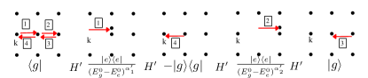
Figure 10: One process chain of energy correction Kato-list with arrow order 1 4 2 3 matching the Kato-list $(\alpha_{1}^{\prime}0\alpha_{2}^{\prime})$.

A.3 Calculation

At last, we turn to the explicit calculation of the energy corrections for the non-degenerate Mott state.eckardt To this end one has to take into account that there are several ways for each arrow diagram to specify the arrow order and each order list is called a process chain. To illustrate this by a concrete example, we consider again the fourth-order diagram in the square lattice. Based on the arguments above, we only store in Fig. 8 the arrow diagram (c), which is characterized by $(rrll)$. If we label each arrow with a number, we have in total four processes. Taking into account all permutations, we have $4!=24$ types of process orders or process chains. In Fig. 10, we show one possible process chain with arrow order 1 4 2 3. All Kato-lists, which satisfy the form $(\alpha_{1}^{\prime}0\alpha_{2}^{\prime})$ with $\alpha_{1}^{\prime}\neq 0$,$\alpha_{2}^{\prime}\neq 0$, contribute to the corresponding energy correction of this process. From Appendix A.1 we know that only the Katolist $(102)$ appears, which can be calculated. For the Mott insulator with filling $n$, the energy correction of this process chain is given by $\frac{(-t\sqrt{n}\sqrt{n+1})^{4}}{(-U)(-1)(-U)^{2}}$, which has to be multiplied with the weight of the Kato-list $(102)$, i.e. with one. After having obtained all the values of the process chains of this arrow diagram, we need to sum them and multiply the result with the weight of this diagram, which is 4.

For calculating the SC energy, we need to consider the degenerate ground state and the algorithm has to be adjusted accordingly.Heil The main idea for calculating the degenerate ground state energy is to construct the effective Hamiltonian matrix perturbatively in the Hilbert space of the degenerate ground states. The diagrams, which have the same end points, belong to the same matrix elements and define an effective hopping process.ss1 Thus in order to get the SC energy, we only need to add all effective hopping matrix elements. Similar to the Mott energy correction, we first need to find out all the process chains and their suitable Kato-lists. As shown in the process chain of Fig. 11, any state $\hat{b}_{i}^{{\dagger}}|\psi_{0}\rangle$ represents a zeroth order ground state, so the process chain matches the Kato-list $(00\alpha_{1}^{\prime})$, and the only Kato-list of this form, which appears, is $(003)$. In case of a particle excitation of a Mott insulator with filling $n$, the energy correction of this process chain turns out to be $\frac{[-t(n+1)]^{2}[-t\sqrt{n(n+1)}]^{2}}{(-1)(-1)(-U)^{3}}$. After having obtained all the values of the process chains of this arrow diagram, we need to sum them and multiply the result with the weight of this diagram, which is 6.

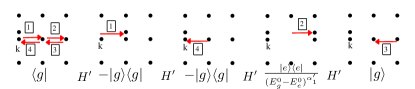
Figure 11: One process chain of SC energy Kato-list with arrow order 1 4 2 3 matches Kato-list $(00\alpha_{1}^{\prime})$.

A.4 Summary

In conclusion, we have to proceed along the following lines in order to calculate the SC energy: At first, we have to generate all process chains of the arrow diagram. Then we have to find the suitable Kato-lists, which we have to calculate. We sum all energy values of the different Kato-lists, in order to get the energy of one process chain. Subsequently, we sum the energies of all process chains and multiply with the weights of the arrow diagrams to determine the energy of the arrow diagrams. At last, we sum the energies of all open and closed arrow diagrams for the SC energy. Finally, by subtracting the energy correction of the particle (or hole) excitation and the Mott state, we obtain the resulting critical line in the respective perturbative order.

Appendix B: : Strong-coupling quantum phase boundary for arbitrary Mott lobe

Here we present our strong-coupling results for the critical lines in Eqs. (2) and (3) of the Bose-Hubbard quantum phase diagram for a general Mott lobe $n$, which were obtained with symbolic calculations up to the 8th order. In order to simplify our notation we give in this appendix both the chemical potential and the hopping matrix element in terms of the energy unit scale of $U$. At first, we consider the Bose-Hubbard chain, i.e. the case $d=1$, where the upper boundary reads

$$\mu_{p}= n-2(n+1)\frac{t}{U}+n^{2}t^{2}+\left(n^{3}+3n^{2}+2n\right)t^{3}+\frac{1}{120}\left(221n^{4}-70n^{3}-559n^{2}-270n\right)t^{4}+\frac{1}{3600}\left(11063n^{5}\right.$$

$$\left.+56453n^{4}+127443n^{3}+114703n^{2}+32650n\right)t^{5}+\frac{1}{9072000}\left(4201738n^{6}-159047706n^{5}-1019369927n^{4}\right.$$

$$\left.-1684710576n^{3}-1075545275n^{2}-246900750n\right)t^{6}+\frac{1}{11430720000}\left(65154949955n^{7}+852816554717n^{6}\right.$$

$$\left.+4617015079493n^{5}+10042635987533n^{4}+10398278064548n^{3}+5217933284246n^{2}+1032937732500n\right)t^{7}$$

$$-\frac{1}{35012981203200000}\left(200810348470291303n^{8}+5778066670166672114n^{7}+43424519219943077927n^{6}\right.$$

$$+134818712387825712764n^{5}+207253111515652899680n^{4}+168130666829189484230n^{3}$$

$$\left.+69538136222775683026n^{2}+11689091525838787500n\right)t^{8}\,,$$ (21)

whereas the lower boundary is given by

$$\mu_{h}= n-1+2nt-\left(n^{2}+2n+1\right)t^{2}+\left(-n^{3}+n\right)t^{3}+\frac{1}{120}\left(-221n^{4}-954n^{3}-977n^{2}-246n-2\right)t^{4}$$

$$+\frac{1}{3600}\left(-11063n^{5}+1138n^{4}-12261n^{3}-39538n^{2}-15076n\right)t^{5}+\frac{1}{9072000}\left(-4201738n^{6}-184258134n^{5}\right.$$

$$\left.+161105327n^{4}+718257312n^{3}+484129979n^{2}+107088822n+54432\right)t^{6}+\frac{1}{11430720000}\left(-65154949955n^{7}\right.$$

$$\left.+396731905032n^{6}-868369700246n^{5}-2530614337602n^{4}-1621977063431n^{3}-467241407430n^{2}\right.$$

$$\left.-45622126368n\right)t^{7}+\frac{1}{35012981203200000}\left(200810348470291303n^{8}-4171583882404341690n^{7}\right.$$

$$+8600742285944529613n^{6}+15634382372668953372n^{5}-3648271187242628015n^{4}-9801914187470665632n^{3}$$

$$\left.-3871241066318288229n^{2}-378804028118746050n+39893821295328\right)t^{8}\,.$$ (22)

Correspondingly, the two-dimensional lattice system turns out to have the upper boundary

$$\mu_{p}= n-4(n+1)t-2(3n^{2}+4n)t^{2}-4\left(11n^{3}+15n^{2}+4n\right)t^{3}-\frac{1}{60}\left(10597n^{4}+24490n^{3}+17857n^{2}+4050n\right)t^{4}$$

$$-\frac{1}{450}\left(941863n^{5}+2188403n^{4}+1638443n^{3}+387253n^{2}-4650n\right)t^{5}-\frac{1}{1512000}\left(17584506524n^{6}\right.$$

$$\left.+56792815090n^{5}+70292096771n^{4}+41746636380n^{3}+12245886137n^{2}+1586224250n\right)t^{6}-\frac{1}{952560000}$$

$$\left(143621438541217n^{7}+482685930471859n^{6}+614916508856545n^{5}+357580517960125n^{4}\right.$$

$$\left.+81552627354718n^{3}-3273334379504n^{2}-3097460700000n\right)t^{7}-\frac{1}{17506490601600000}$$

$$\left(15828728653296464701673n^{8}+66223539683880680581462n^{7}+114520168944419866201057n^{6}\right.$$

$$+106687922443046182561852n^{5}+59150401403670755097004n^{4}+20678487502333510720450n^{3}$$

$$\left.+4647036608792957074250n^{2}+556471872345686887500n\right)t^{8}\,,$$ (23)

and the lower boundary is determined by

$$\mu_{h}= n-1+4nt+\left(6n^{2}+4n-2\right)t^{2}+4n(n+1)(11n+7)t^{3}+\frac{1}{60}\left(10597n^{4}+17898n^{3}+7969n^{2}+582n\right.$$

$$\left.-86\right)t^{4}+\frac{1}{450}\left(941863n^{5}+2520912n^{4}+2303461n^{3}+816288n^{2}+91876n\right)t^{5}+\frac{1}{1512000}\left(17584506524n^{6}\right.$$

$$\left.+48714224054n^{5}+50095619181n^{4}+23183730284n^{3}+4598004583n^{2}+376989662n-3186288\right)t^{6}$$

$$+\frac{1}{952560000}\left(143621438541217n^{7}+522664139316660n^{6}+734851135390948n^{5}+503463418187310n^{4}\right.$$

$$\left.+173427383585083n^{3}+27374449536030n^{2}+1602049522752n\right)t^{7}+\frac{1}{17506490601600000}$$

$$\left(15828728653296464701673n^{8}+60406289542491037031922n^{7}+94159793449556113777667n^{6}\right.$$

$$+76147562446580745727476n^{5}+33700440149666544069539n^{4}+8032188219063211012704n^{3}$$

$$\left.+947361190459842328401n^{2}+50197343417953427898n-85891426017677280\right)t^{8}\,.$$ (24)

Finally, the upper boundary of a three-dimensional Mott lobe reads

$$\mu_{p}= n+(-6n-6)t-3\left(7n^{2}+8n\right)t^{2}+\left(-231n^{3}-333n^{2}-102n\right)t^{3}+\frac{1}{8}\left(-20683n^{4}-42646n^{3}-26919n^{2}\right.$$

$$\left.-4990n\right)t^{4}+\frac{1}{240}\left(-9450991n^{5}-23212861n^{4}-19367531n^{3}-6129431n^{2}-523770n\right)t^{5}$$

$$+\frac{1}{3024000}\left(-1612512639802n^{6}-4903150529490n^{5}-5568888652747n^{4}-2895859756680n^{3}-673691826835n^{2}\right.$$

$$\left.-56132922750n\right)t^{6}+\frac{1}{1270080000}\left(-11585180188993081n^{7}-40169594556544231n^{6}-54166855276590991n^{5}\right.$$

$$\left.-35546615871621511n^{4}-11500224469294300n^{3}-1582089821730130n^{2}-46040315017500n\right)t^{7}$$

$$+\frac{1}{11670993734400000}\left(-1591704030486631948004941n^{8}-6411307825175115072269186n^{7}\right.$$

$$-10477219584627901596466499n^{6}-8903631755605628211005096n^{5}-4192954829256834761500718n^{4}$$

$$\left.-1081820439715328380764170n^{3}-143411169994732620393730n^{2}-8530598518867251187500n\right)t^{8}\,,$$ (25)

where the low boundary is characterized by

$$\mu_{h}= n-1+6nt+3\left(7n^{2}+6n-1\right)t^{2}+\left(231n^{3}+360n^{2}+129n\right)t^{3}+\frac{1}{8}\left(20683n^{4}+40086n^{3}+23079n^{2}\right.$$

$$\left.+3642n-34\right)t^{4}+\frac{1}{240}\left(9450991n^{5}+24042094n^{4}+21025997n^{3}+7205906n^{2}+771012n\right)t^{5}+\frac{1}{3024000}$$

$$\left(1612512639802n^{6}+4771925309322n^{5}+5240825602327n^{4}+2598442355448n^{3}+555628775407n^{2}\right.$$

$$\left.+38549263230n-50089536\right)t^{6}+\frac{1}{1270080000}\left(11585180188993081n^{7}+40926666766407336n^{6}\right.$$

$$+56438071906180306n^{5}+38225048777927814n^{4}+13071729232591381n^{3}+2052306743024850n^{2}$$

$$\left.+109040959595232n\right)t^{7}+\frac{1}{11670993734400000}\left(1591704030486631948004941n^{8}\right.$$

$$+6322324418717940511770342n^{7}+10165777662027790634720545n^{6}+8457647130735753938417688n^{5}$$

$$+3856598073582426484397083n^{4}+937724839936122043372908n^{3}+107903564700275910537495n^{2}$$

$$\left.+4285936758470495239062n-1004648837988860064\right)t^{8}\,.$$ (26)

References

- (1) E. Dagotto. Correlated electrons in high-temperature superconductors. Rev. Mod. Phys. 66, 763 (1994).
- (2) M. P. A. Fisher, P. B. Weichman, G. Grinstein, and D. S. Fisher. Boson localization and the superfluid-insulator transition. Phys. Rev. B 40, 546 (1989).
- (3) D. Jaksch, C. Bruder, J. I. Cirac, C. W. Gardiner, and P. Zoller. Cold Bosonic Atoms in Optical Lattices. Phys. Rev. Lett. 81, 3108 (1998).
- (4) M. Greiner, O. Mandel, T. Esslinger, T. W. Hänsch, and I. Bloch. Quantum phase transition from a superfluid to a Mott insulator in a gas of ultracold atoms. Nature (London) 415, 39 (2002).
- (5) S. Baier, M. J. Mark, D. Petter, K. Aikawa, L. Chomaz, Zi Cai, M. Baranov, P. Zoller, and F. Ferlaino. Extended Bose-Hubbard Models with Ultracold Magnetic Atoms. Science 352, 201 (2016).
- (6) B. Yan, S. A. Moses, B. Gadway, J. P. Covey, K. R. A. Hazzard, A. M. Rey, D. S. Jin, and J. Ye. Observation of dipolar spin-exchange interactions with lattice-confined polar molecules. Nature (London) 501, 521 (2013).
- (7) P. Schau, M. Cheneau, M. Endres, T. Fukuhara, S. Hild, A. Omran, T. Pohl, C. Gross, S. Kuhr, and I. Bloch. Observation of Spatially Ordered Structures in a Two-Dimensional Rydberg Gas. Nature (London) 491, 87 (2012).
- (8) X.-F. Zhang, R. Dillenschneider, Y. Yu, and S. Eggert. Supersolid phase transitions for hard-core bosons on a triangular lattice. Phys. Rev. B 84, 174515 (2011).
- (9) D. Yamamoto, I. Danshita, and C. A. R. Sá de Melo. Dipolar bosons in triangular optical lattices: Quantum phase transitions and anomalous hysteresis. Phys. Rev. A 85, 021601(R) (2012).
- (10) L. Bonnes and S. Wessel. Generic first-order versus continuous quantum nucleation of supersolidity. Phys. Rev. B 84, 054510 (2011).
- (11) X.-F. Zhang, S. Hu, A. Pelster, and S. Eggert. Quantum Domain Walls Induce Incommensurate Supersolid Phase on the Anisotropic Triangular Lattice. Phys. Rev. Lett. 117, 193210 (2016).
- (12) X.-F. Zhang, Q. Sun, Y.-C. Wen, W.-M. Liu, S. Eggert, and A.-C. Ji. Rydberg Polaritons in a Cavity: A Superradiant Solid. Phys. Rev. Lett. 110, 090402 (2013).
- (13) X.-F. Zhang and S. Eggert. Chiral Edge States and Fractional Charge Separation in a System of Interacting Bosons on a Kagome Lattice. Phys. Rev. Lett. 111, 147201 (2013).
- (14) J. K. Freericks and H. Monien. Strong-coupling expansions for the pure and disordered Bose-Hubbard model. Phys. Rev. B 53, 2691 (1996).
- (15) I. Hen, M. Iskin, and M. Rigol. Phase diagram of the hard-core Bose-Hubbard model on a checkerboard superlattice. Phys. Rev. B 81, 064503 (2010).
- (16) M. Iskin. Strong-coupling expansion for the two-species Bose-Hubbard model. Phys. Rev. A 82, 033630 (2010).
- (17) M. Iskin. Mean-field theory for the Mott-insulator–paired-superfluid phase transition in the two-species Bose-Hubbard model. Phys. Rev. A 82, 055601 (2010).
- (18) X.-F. Zhang, Y.-C. Wen, and Y. Yu. Three-body interactions on a triangular lattice. Phys. Rev. B 83, 184513 (2011).
- (19) A. Eckardt. Process-chain approach to high-order perturbation calculus for quantum lattice models. Phys. Rev. B 79, 195131 (2009).
- (20) N. Teichmann, D. Hinrichs, M. Holthaus, and A. Eckardt. Process-chain approach to the Bose-Hubbard model: Ground-state properties and phase diagram. Phys. Rev. B 79, 224515 (2009).
- (21) T. Kato. On the Convergence of the Perturbation Method. I. Prog. Theor. Phys. 4, 514 (1949).
- (22) F. E. A. dos Santos and A. Pelster. Quantum phase diagram of bosons in optical lattices. Phys. Rev. A 79, 013614 (2009).
- (23) T. Wang, X.-F. Zhang, S. Eggert, and A. Pelster. Generalized Effective Potential Landau Theory for Bosonic Superlattices. Phys. Rev. A 87, 063615 (2013).
- (24) F. Wei, J. Zhang, and Y. Jiang. Quantum phase diagram and time-of-flight absorption pictures of an ultracold Bose system in a square optical superlattice. Eur. Phys. Lett. 113, 16004 (2016).
- (25) D. Hinrichs, A. Pelster, and M. Holthaus. Perturbative calculation of critical exponents for the Bose-Hubbard model. Appl. Phys. B 113, 57 (2013).
- (26) C. Heil and W. von der Linden. Strong coupling expansion for the Bose-Hubbard and Jaynes-Cummings lattice models. J. Phys.: Cond. Mat. 24, 295601 (2012).
- (27) N. Elstner and H. Monien. Dynamics and thermodynamics of the Bose-Hubbard model. Phys. Rev. B 59, 12184 (1999).
- (28) N. Teichmann and D. Hinrichs. Scaling property of the critical hopping parameters for the Bose-Hubbard model. Eur. Phys. J. B 71, 219 (2009).
- (29) M. P. Gelfand and R. R. P. Singh. High-order convergent expansions for quantum many particle systems. Adv. Phys. 49, 93 (2000).
- (30) S. Sachdev. Quantum Phase Transitions, 2nd edn. (Cambridge University Press, Cambridge, 2011).
- (31) T. D. Kühner and H. Monien. Phases of the one-dimensional Bose-Hubbard model. Phys. Rev. B 58, R14741 (1998).
- (32) G. A. Baker and P. Graves-Morris. Padé Approximants, 2nd edn. (Cambridge University Press, Cambridge, 2016).
- (33) S. Ejima, H. Feheske, and F. Gebhard. Dynamic properties of the one-dimensional Bose-Hubbard model. Euro. Phys. Lett 93, 554 (2011).
- (34) A. M. Lauchli and C. Kollath. Spreading of correlations and entanglement after a quench in the one-dimensional Bose-Hubbard model. J. Stat. Mech. P05018 (2008).
- (35) I. Danshita and A. Polkovnikov. Superfluid-to-Mott-insulator transition in the one-dimensional Bose-Hubbard model for arbitrary integer filling factors. Phys. Rev. A 84, 063637(2011).
- (36) B. Capogrosso-Sansone, S. G. Soyler, N. V. Prokofev, and B. Svistunov. Monte Carlo study of the two-dimensional Bose-Hubbard model. Phys. Rev. A 77, 015602 (2008).
- (37) B. Capogrosso-Sansone, N. V. Prokof’ev, and B. V. Svistunov. Phase diagram and thermodynamics of the three-dimensional Bose-Hubbard model. Phys. Rev. B 75, 134302 (2007).
- (38) J. Zinn-Justin. Quantum field theory and critical phenomena, 4th edn. (Oxford University Press, Oxford, 2002).
- (39) H. Kleinert and V. Schulte-Frohlinde. Critical properties of theories (World Scientific, Singapore, 2001).
- (40) M. Campostrini, M. Hasenbusch, A. Pelissetto, P. Rossi, and E. Vicari. Critical behavior of the three-dimensional XY universality class. Phys. Rev. B 63, 214503 (2001).
- (41) T. Wang, X.-F. Zhang, S. Eggert, and A. Pelster. Tuning the Quantum Phase Transition of Bosons in Optical Lattices via Periodic Modulation of s-Wave Scattering Length. Phys. Rev. A 90, 013633 (2014).
-
(42)
See Supplemental Material for the Matlab code which calculates the
high-order strong-coupling expansion for different fillings in a square lattice:
http://power.itp.ac.cn/~zxf/source/HSCE.m - (43) X.-F. Zhang, T. Wang, S. Eggert, and A. Pelster. Tunable anisotropic superfluidity in an optical kagome superlattice. Phys. Rev. B 92, 014512 (2015).
- (44) C.-L. Hung, X. Zhang, N. Gemelke, and C. Chin. Observation of scale invariance and universality in two-dimensional Bose gases. Nature 470,236 (2011).
- (45) H. Ott. Single atom detection in ultracold quantum gases: a review of current progress. Rep. Prog. Phys. 79, 054401 (2016).
- (46) W. S. Bakr, J. I. Gillen, A. Peng, S. Fölling, and M. Greiner. A quantum gas microscope for detecting single atoms in a Hubbard-regime optical lattice. Nature (London) 462, 74 (2009)
- (47) B. Santra and H. Ott. Scanning electron microscopy of cold gases. J. Phys. B: At. Mol. Opt. Phys. 48 122001 (2015).