Hi-Fi: Hierarchical Feature Integration for Skeleton Detection

Abstract

In natural images, the scales (thickness) of object skeletons may dramatically vary among objects and object parts, making object skeleton detection a challenging problem. We present a new convolutional neural network (CNN) architecture by introducing a novel hierarchical feature integration mechanism, named Hi-Fi, to address the skeleton detection problem. The proposed CNN-based approach has a powerful multi-scale feature integration ability that intrinsically captures high-level semantics from deeper layers as well as low-level details from shallower layers. By hierarchically integrating different CNN feature levels with bidirectional guidance, our approach (1) enables mutual refinement across features of different levels, and (2) possesses the strong ability to capture both rich object context and high-resolution details. Experimental results show that our method significantly outperforms the state-of-the-art methods in terms of effectively fusing features from very different scales, as evidenced by a considerable performance improvement on several benchmarks. Code is available at http://mmcheng.net/hifi.

1 Introduction

Object skeletons are defined as the medial axis of foreground objects surrounded by closed boundaries Blum (1967). Complementary to object boundaries, skeletons are shape-based descriptors which provide a compact representation of both object geometry and topology. Due to its wide applications in other vision tasks such as shape-based image retrieval Demirci et al. (2006); Sebastian et al. (2004), and human pose estimation Girshick et al. (2011); Shotton et al. (2013); Sun et al. (2012). Skeleton detection is extensively studied very recently  Shen et al. (2017); Ke et al. (2017); Tsogkas and Dickinson (2017).

\begin{overpic}[width=433.62pt]{figures/fig1.pdf} \put(2.0,10.0){(b)} \put(2.0,33.0){(a)} \put(62.0,10.0){(c)} \end{overpic}

Figure 1: Skeleton detection is facing a more challenging scale space problem: (a) object boundaries can be detected with filters of similar size (green boxes); (b) only filters a bit larger than the skeleton scale (green boxes) can capture proper context for skeleton detection; both improper big or small (red boxes) cannot perceive skeletons well; (c) compared with boundary detection and semantic segmentation, skeleton detection requires inhomogeneous feature levels.

Because the skeleton scales (thickness) are unknown and may vary among objects and object parts, skeleton detection has to deal with a more challenging scale space problem Shen et al. (2016b) compared with boundary detection, as shown in Fig. 1. Consequently, it requires the detector to capture broader context for detecting potential large-scale (thick) skeletons, and also possess the ability to focus on local details in case of small-scale (thin) skeletons.

\begin{overpic}[width=390.25534pt]{figures/arch_feat_integration_big} \put(9.0,-2.0){(a)} \put(32.0,-2.0){(b)} \put(56.0,-2.0){(c)} \put(77.0,-2.0){(d)} \end{overpic}

Figure 2: Different multi-scale CNN feature fusing methods: (a) side-outputs as independent detectors at different scales Xie and Tu (2015); Shen et al. (2016b); (b) deep-to-shallow refinement Ke et al. (2017) that brings high-level semantics to lower layers; (c) directly fuse all feature levels at once; (d) our hierarchical integration architecture, which enables bidirectional mutual refinement across low/high level features by recursive feature integration.

Performing multi-level feature fusion has been a primary trend in pixel-wise dense prediction such as skeleton detection Ke et al. (2017) and saliency detection Zhang et al. (2017); Hou et al. (2018). These methods fuse CNN features of different levels in order to obtain more powerful representations. The disadvantage of existing feature fusion methods is that they perform only deep-to-shallow refinement, which provides shallow layers the ability of perceiving high-level concepts such as object and image background. Deeper CNN features in these methods still suffer from low-resolution, which is a bottleneck to the final detection results.

In this paper we introduce hierarchical feature integration (Hi-Fi) mechanism with bidirectional guidance. Different from existing feature fusing solutions, we explicitly enable both deep-to-shallow and shallow-to-deep refinement to enhance shallower features with richer semantics, and enrich deeper features with higher resolution information. Our architecture has two major advantages compared with existing alternatives:

Bidirectional Mutual Refinement.

Different from existing solutions illustrated in Fig. 2 (a) and Fig. 2 (b) where different feature levels work independently or allow only deep-to-shallow guidance, our method Fig. 2 (d) enables not only deep-to-shallow but also shallow-to-deep refinement, which allows the high-level semantics and low-level details to mutually help each other in a bidirectional fashion.

Hierarchical Integration.

There are two alternatives for mutual integration: directly fusing all levels of features as shown in Fig. 2 (c), or hierarchically integrating them as shown in Fig. 2 (d). Due to the significant difference between faraway feature levels, directly fusing all of them might be very difficult. We take the second approach as inspired by the philosophy of ResNet He et al. (2016), which decomposes the difficult problem into much easier sub-problems: identical mapping and residual learning. We decompose the feature integration into easier sub-problems: gradually combining nearby feature levels. Because optimizing combinations of close features is more practical and easier to converge due to their high similarity. The advantage of hierarchical integration over directly fusing all feature levels is verified in the experiments (Fig. 9).

2 Related Work

Skeleton Detection.

Numerous models have been proposed for skeleton detection in the past decades. In general, they can be divided into three categories: (a) early image processing based methods, these methods localize object skeleton based on the geometric relationship between object skeletons and boundaries; (b) learning based methods, by designing hand-crafted image features, these methods train a machine learning model to distinguish skeleton pixels from non-skeleton pixels; (c) recent CNN-based methods which design CNN architectures for skeleton detection.

Most of the early image processing based methods  Morse et al. (1993); Jang and Hong (2001) rely on the hypothesis that skeletons lie in the middle of two parallel boundaries. A boundary response map is first calculated (mostly based on image gradient), then skeleton pixels can be localized with the geometric relationship between skeletons and boundaries. Some researchers then investigate learning-based models for skeleton detection. They train a classifier Tsogkas and Kokkinos (2012) or regressor Sironi et al. (2014) with hand-crafted features to determine whether a pixel touches the skeleton. Boundary response is very sensitive to texture and illumination changes, therefore image processing based methods can only deal with images with simple backgrounds. Limited by the ability of traditional learning models and representation capacity of hand-crafted features, they cannot handle objects with complex shapes and various skeleton scales.

More recently many researchers have been exploiting the powerful convolutional neural networks (CNNs) for skeleton detection and significant improvements have been achieved on several benchmarks. HED Xie and Tu (2015) introduces side-output that is branched from intermediate CNN layers for multi-scale edge detection. FSDS Shen et al. (2016b) then extends side-output to be scale-associated side-output, in order to tackle the scale-unknown problem in skeleton detection. The side-output residual network (SRN) Ke et al. (2017) exploits deep-to-shallow residual connections to bring high-level, rich semantic features to shallower side-outputs with the purpose of making the shallower side-outputs more powerful to distinguish real object skeletons from local reflective structures.

Multi-Scale Feature Fusing in CNNs.

CNNs naturally learn low/mid/high level features in a shallow to deep layer fashion. Low-level features focus more on local detailed structures, while high-level features are rich in conceptual semantics Zeiler and Fergus (2014). Pixel-wise dense prediction tasks such as skeleton detection, boundary detection and saliency detection require not only high-level semantics but also high-resolution predictions. As pooling layers with strides down-sample the feature maps, deeper CNN features with richer semantics are always with lower resolution.

Many researchers Ke et al. (2017); Zhang et al. (2017); Hou et al. (2018) try to fuse deeper rich semantic CNN features with shallower high-resolution features to overcome this semantic vs resolution conflict. In SRN, Ke et. al. Ke et al. (2017) connected shallower side-outputs with deeper ones to refine the shallower side-outputs. As a result, the shallower side-outputs become much cleaner because they are capable of suppressing non-object textures and disturbances. Shallower side-outputs of methods without deep-to-shallow refinement such as HED Xie and Tu (2015) and FSDS Shen et al. (2016b) are filled with noises.

A similar strategy has been exploited in DSS Hou et al. (2018) and Amulet Zhang et al. (2017) for saliency detection, and a schema of these methods with deep-to-shallow refinement can be summarized as Fig. 2 (b). The problem of these feature fusion methods is that they lack the shallow-to-deep refinement, the deeper side-outputs still suffer from low-resolution. For example, DSS has to empirically drop the last side-output for its low-resolution.

\begin{overpic}[width=390.25534pt]{figures/arch_fsds_srn_hifi2_h-cropped} \put(37.0,10.0){Hi-Fi-1} \put(60.5,10.0){Hi-Fi-2} \end{overpic}

Figure 3: Architecture of our proposed Hi-Fi network. All side-outputs (SOs, marked with rounded square box) are supervised by skeletons within their receptive fields (numbers on top of SOs indicate their receptive fields). Features of neighbouring feature levels are integrated to enable mutual refinement, and a lateral feature hierarchy is obtained with recursively integrating neighbouring features.

3 Hi-Fi: Hierarchical Feature Integration

3.1 Overall Architecture

We implement the proposed Hi-Fi architecture based on the VGG16 Simonyan and Zisserman (2015) network, which has 13 convolutional layers and 2 fully connected layers. The conv-layers in VGG network are divided into 5 groups: conv1-x, …, conv5-x, and there are 2$\sim$3 conv-layers in a group. There are pooling layers with $stride=2$ between neighbouring convolution groups.

In HED, the side-outputs connect only with the last conv-layer of each group. RCF (Richer Convolution Features) Liu et al. (2017) connects a side-output to all layers of a convolutional group. We follow this idea to get more powerful convolutional features. The overall architecture of Hi-Fi is illustrated in Fig. 3, convolutional groups are distinguished by colors, and pooling layers are omitted.

3.2 Hierarchical Feature Integration

A detailed illustration of the proposed feature integration procedure is shown in Fig. 4. Feature maps to be integrated are branched from the primary network stream through a ($1\times 1$) convolutional layer (dotted boxes marked with (a)) on top of an interior convolutional layer. These feature maps are further integrated with element-wise sum (box marked with (c)). The final scale-associated side-output (box marked with (d)) is produced by a ($1\times 1$) convolution. Note that due to the existence of pooling layers, deeper convolutional feature maps are spatially smaller than shallower ones. Upsampling (box marked with (b)) is required to guarantee all feature maps to be integrated are of the same size.

Ideally, the feature integration can be recursively performed until the last integrated feature map contains information from all convolution layers (conv1-1 $\sim$ conv5-3). However, limited by the memory of our GPUs and the training time, we end up with two level integration (Fig. 3 ‘Hi-Fi-2’).

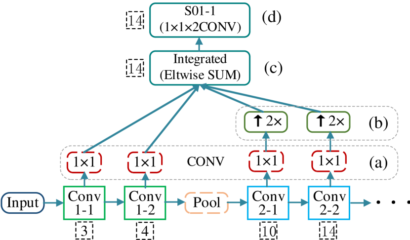
Figure 4: Illustration of feature integration: (a) feature maps to be integrated are firstly produced by a (1$\times$1) convolution; (b) deeper features are upsampled before integration; (c) the integration is implemented by an element-wise sum; (d) side-outputs are built on top of the integrated features with a (1$\times$1) convolution.

Bidirectional Refinement.

We explain the proposed bidirectional mutual refinement by comparing it with existing architectures: FSDS Shen et al. (2016b) and SRN Ke et al. (2017). As shown in Fig. 5, side-outputs (SOs) of FSDS are working independently, there is no cross talk between features of different levels. As a result, FSDS has noisy shallow SOs and low-resolution deeper SOs. SRN then introduces deep-to-shallow refinement by bringing deep features to shallow SOs. As shown in Fig. 5, shallower SOs of SRN are much cleaner than that of FSDS. Despite the improvement, deeper SOs in SRN are still suffering from low-resolution, which limits the quality of the final fused result.

In our architecture SOs are built on top of an integration of nearby feature levels, and the “nearby feature integration” is recursively performed. In testing phase, SOs will receive information from both deeper and shallower sides; and in training phase, gradient from SOs will back-prop to both as well. In other words, our approach explicitly enables not only deep-to-shallow but also shallow-to-deep refinement. It is obviously shown in Fig. 5 that Hi-Fi obtains cleaner shallower SOs than FSDS, and at the same time has much more high-resolution deeper SOs than SRN. Consequently, we gain a strong quality improvement in the final fused result.

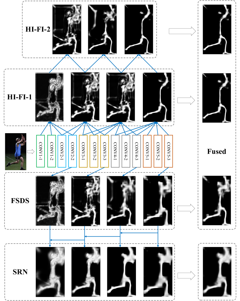
Figure 5: Illustration of Hi-Fi, FSDS Shen et al. (2016b) and SRN Ke et al. (2017).

3.3 Formulation

Here we formulate our approach for skeleton detection. Skeleton detection can be formulated as a pixel-wise binary classification problem. Given an input image $X=\{x_{j},j=1,...,|X|\}$, the goal of skeleton detection is to predict the corresponding skeleton map $\hat{Y}=\{\hat{y_{j}},j=1,...,|X|\}$, where $\hat{y_{j}}\in\{0,1\}$ is the predicted label of pixel $x_{j}$. $\hat{y_{j}}=1$ means pixel $x_{j}$ is predicted as a skeleton point, otherwise, pixel $x_{j}$ is the background.

Ground-truth Quantization.

Following FSDS Shen et al. (2016b), we supervise the side-outputs with ‘scale-associated’ skeleton ground-truths. To differentiate and supervise skeletons of different scales, skeletons are quantized into several classes according to their scales. The skeleton scale is defined as the distance between a skeleton point and its nearest boundary point. Assume $S=\{s_{j},j=1,...,|X|\}(s_{j}\in R)$ is the skeleton scale map, where $s_{j}$ represents the skeleton scale of pixel $x_{j}$. When $x_{j}$ is the background, $s_{j}=0$. Let $Q=\{q_{j},j=1,...,|X|\}$ be the quantized scale map, where $q_{j}$ is the quantized scale of pixel $x_{j}$. The quantized scale $q_{j}$ can be obtained by:

$$q_{j}=\begin{cases}m&\text{if $r_{m-1}<s_{j}\leqslant r_{m}$}\\ 0&\text{if $s_{j}=0$ or $s_{j}>r_{M}$},\end{cases}$$ (1)

where $r_{m}$ ($m=1,...,M$) is the receptive field of the $m$-th side-output (SO-$m$), with $r_{0}=0$, and $M$ is the number of side-outputs. For instance, pixel $x_{j}$ with scale $s_{j}=39$ is quantized as $q_{j}=3$, because $14=r_{2}<s_{j}\leqslant r_{3}=40$ (receptive fields of side-outputs are shown in Fig. 3 with numbers-in-boxes). All background pixels ($s_{j}=0$) and skeleton points out of scope of the network ($s_{j}>r_{M}$) are quantized as 0.

Supervise the Side-outputs.

Scale-associated side-output is only supervised by the skeleton with scale smaller than its receptive field. We denote ground-truth as $G^{m}=\{g^{m}_{j},j=1,...,|X|\}$, which is used to supervise SO-$m$. $G^{m}$ is modified from $Q$ with all quantized values larger than $m$ set to zero. $g^{m}_{j}$ can be obtained from $Q$ by:

$$g^{m}_{j}=\begin{cases}q_{j}&\text{if $q_{j}<m$}\\ 0&\text{otherwise}.\end{cases}$$ (2)

Supervising side-outputs with the quantized skeleton map turns the original binary classification problem into a multi-class problem.

Fuse the Side-outputs.

Suppose $P^{m}=\{p^{m}_{j,k},j=1,...,|X|,k=0,...,K^{m}\}$ is the predicted probability map of SO-$m$, in which $K^{m}$ is the number of quantized classes SO-$m$ can recognise. $p^{m}_{j,k}$ means the probability of pixel $x_{j}$ belonging to a quantized class #$k$, and index $j$ is over the spatial dimensions of the input image $X$. Obviously we have $\sum_{k=0}^{K^{m}}p^{m}_{j,k}=1$.

We fuse the probability maps from different side-outputs $P^{m}(m=1,...,M)$ with a weighted summation to obtain the final fused prediction $P=\{p_{j,k}\}$:

$$p_{j,k}=\sum_{m}w_{mk}\cdot p^{m}_{j,k},$$ (3)

where $p_{j,k}$ is the fused probability that pixel $x_{j}$ belongs to quantized class #$k$, $w_{mk}$ is the credibility of side-output $m$ on quantized class #$k$. Eq. (3) can be implemented with a simple ($1\times 1$) convolution.

Loss Function and Optimization.

We simultaneously optimize all the side-outputs $P^{m}(m=1,...,M)$ and the fused prediction $P$ in an end-to-end way. In HED Xie and Tu (2015), Xie and Tu introduce a class-balancing weight to address the problem of positive/negative unbalancing in boundary detection. This problem still exists in skeleton detection because most of the pixels are background. We use the class-balancing weight to offset the imbalance between skeletons and the background. Specifically, we define the balanced softmax loss $l(P,G)$ as:

$$\begin{split}l(P,G)=\sum_{j}\Big{[}-\beta^{m}\sum_{k\neq 0}\log(p^{m}_{j,k})1(g^{m}_{j}==k)-\\ (1-\beta^{m})\log(p^{m}_{j,0})1(g^{m}_{j}==0)\Big{]},\end{split}$$ (4)

where $P=h(X|\Theta)$ is the prediction from CNN, $G$ is the ground-truth, and $m$ is the index of side-outputs. $h(X|\Theta)$ is the model hypothesis taking image $X$ as input, parameterized by $\Theta$. $\beta^{m}=\left[\sum_{j=1}^{|X|}1(g^{m}_{j}\neq 0)\right]/|X|$ is a balancing factor, where $1(\cdot)$ is an indicator. The overall loss function can be expressed as follow:

$$\begin{split}\mathcal{L}\big{(}h(X|\Theta),G\big{)}&=\mathcal{L}_{\text{side}}+\mathcal{L}_{\text{fuse}}\\ &=\sum_{m=1}^{M}l(P^{m},G^{m})+l(P,Q),\end{split}$$ (5)

where $P^{m}$ and $G^{m}$ are prediction/ground-truth of SO-$m$ respectively, $G$ is the ground-truth of final fused output $P$.

All the parameters including the fusing weight $w_{mk}$ in Eq. (3) are part of $\Theta$. We can obtain the optimal parameters by a standard stochastic gradient descent (SGD):

$$(\Theta)^{*}=\operatorname*{argmin}\mathcal{L}.$$ (6)

Detect Skeleton with Pretrained Model.

Given trained parameters $\Theta$, the skeleton response map $\hat{Y}=\{\hat{y}_{j},j=1,...,|X|\}$ is obtained via:

$$\hat{y}_{j}=1-p_{j,0},$$ (7)

where $\hat{y}_{j}\in[0,1]$ indicates the probability that pixel $x_{j}$ belongs to the skeleton.

4 Experiments and Analysis

In this section, we discuss the implementation details and report the performance of the proposed method on several open benchmarks.

4.1 Datasets

The experiments are conducted on four popular skeleton datasets: WH-SYMMAX Shen et al. (2016a), SK-SMALL Shen et al. (2016b), SK-LARGE Shen et al. (2017) and SYM-PASCAL Ke et al. (2017). Images of these datasets are selected from other semantic segmentation datasets with human annotated object segmentation masks, and the skeleton ground-truths are extracted from segmentations. Objects of SK-SMALL and SK-LARGE are cropped from MSCOCO dataset with ‘well defined’ skeletons , and there is only one object in each image. SYM-PSCAL selects images from the PASCAL-VOC2012 dataset without cropping and here may be multiple objects in an image.

Some representative example images and corresponding skeleton ground-truths of these datasets are shown in Fig. 6.

\begin{overpic}[width=433.62pt]{figures/dataset-examples.png} \put(1.0,-4.0){\scriptsize{(a) SYM-PASCAL}} \put(26.0,-4.0){\scriptsize{(b) SK-SMALL}} \put(54.0,-4.0){\scriptsize{(c) SK-LARGE}} \put(79.0,-4.0){\scriptsize{(d) WH-SYMMAX}} \end{overpic}

Figure 6: Example images and corresponding skeleton ground-truths (red curves) of several skeleton datesets.

4.2 Implementation Details

We implement the proposed architecture based on the openly available caffe Jia et al. (2014) framework. The hyper-parameters and corresponding values are: base learning rate ($10^{-6}$), mini-batch size (1), momentum (0.9) and maximal iteration (40000). We decrease the learning rate every 10,000 iterations with factor 0.1.

We perform the same data augmentation operations with FSDS for fair comparison. The augmentation operations are: (1) random resize images (and gt maps) to 3 scales (0.8, 1, 1.2), (2) random left-right flip images (and gt maps); and (3) random rotate images (and gt maps) to 4 angles (0, 90, 180, 270).

4.3 Evaluation Protocol

The skeleton response map $\hat{Y}$ is obtained through Eq. (7), to which a standard non-maximal suppression (NMS) is then applied to obtain the thinned skeleton map for evaluation. We evaluate the performance of the thinned skeleton map $\hat{Y}$ in terms of F-measure= $2\frac{Precision\cdot Recall}{Precision+Recall}$ as well as the precision recall curve (PR-curve) w.r.t ground-truth $G$. By applying different thresholds to $\hat{Y}$, a series of precision/recall pairs are obtained to draw the PR-curve. The F-measure is obtained under the optimal threshold over the whole dataset.

4.4 Skeleton Detection

We test our method on four aforementioned datasets. Example images and ground-truths of these datasets are shown in Fig. 6, some detection results by different approaches are shown in  Fig. 8. Similar to RCF Liu et al. (2017) we perform multi-scale detection by resizing input images to different scales (0.5, 1, 1.5) and average their results. We compare the proposed approach with other competitors including one learning based method MIL Tsogkas and Kokkinos (2012), and several recent CNN-based methods: FSDS Shen et al. (2016b), SRN Ke et al. (2017), HED Xie and Tu (2015), RCF Liu et al. (2017)). FSDS and SRN are specialized skeleton detectors, HED and RCF are developed for edge detection. Quantitative results are shown in Fig. 7 and Tab.1, our proposed method outperforms the competitors in both terms of F-measure and PR-curve. Some representative detection results are shown in Fig. 8.

Comparison results in Tab. 1 reveal that with 1st-level hierarchical integration (Hi-Fi-1), our method (Hi-Fi-1) already outperforms others with a significant margin. Moreover, by integrating 1st-level integrated features we obtain the 2nd-level integration (Hi-Fi-2) and the performance witnesses a further improvement (Limited by the GPU memory, we didn’t implement Hi-Fi-3). Architecture details of Hi-Fi-1 and Hi-Fi-2 are illustrated in Fig. 3.

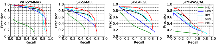
Figure 7: Precision Recall curves of recent CNN-based methods HED Xie and Tu (2015), RCF Liu et al. (2017), FSDS Shen et al. (2016b), SRN Ke et al. (2017) and one learning based method MIL Tsogkas and Kokkinos (2012).

\begin{overpic}[width=433.62pt]{figures/detection-examples} \put(0.2,-4.0){Ground-truth} \put(32.0,-4.0){FSDS} \put(58.0,-4.0){SRN} \put(77.0,-4.0){Ours (Hi-Fi)} \end{overpic}

Figure 8: Representative detection results. Our detected skeletons are more continuous and finer (thinner) than others.

Methods	WH- SYMMAX	SK- SMALL	SK-L ARGE	SYM- PASCAL
MIL	0.365	0.392	0.293	0.174
HED	0.732	0.542	0.497	0.369
RCF	0.751	0.613	0.626	0.392
FSDS	0.769	0.623	0.633	0.418
SRN	0.780	0.632	0.640	0.443
Hi-Fi	0.805	0.681	0.724	0.454

Table 1: F-measure comparison between different methods on four popular skeleton datasets. Our proposed Hi-Fi network outperforms other methods with an evident margin.

4.5 Ablation Study

We do ablation study on SK-LARGE dataset to further probe the proposed method.

Different Feature Integrating Mechanisms.

We compare different feature integrating mechanisms including: (1) FSDS Shen et al. (2016b), (2) SRN  Ke et al. (2017) with deep-to-shallow refinement, (3) Hi-Fi-1 with 1 level hierarchical integration ( Fig. 3 (Hi-Fi-1)), and (4) Hi-Fi-2 with 2 level hierarchical integration ( Fig. 3 (Hi-Fi-2)). Results are shown in Tab. 2.

FSDS	SRN	Hi-Fi-1	Hi-Fi-2
0.633	0.640	0.703	0.724

Table 2: Performance of different feature integration mechanisms.

Hierarchical Integration versus Direct Fusing.

To further justify the proposed hierarchical feature integration mechanism (Hi-Fi), we compare the proposed Hi-Fi network with another architecture described in Fig. 2 (c), which fuses features from all levels together at once.

The comparison results shown in Fig. 9 support our claim that “learning an integration of nearby feature levels is easier than learning combination of features of all levels”, as evidenced by a faster convergence and better converged performance.

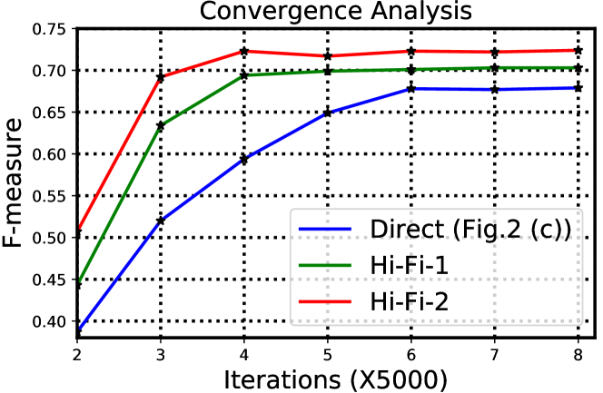
Figure 9: Hierarchical Feature Integration (Hi-Fi) versus Direct Fusing (Fig. 2 (c)).

Integrating $K$ Feature Levels at Each Step.

We also test models that fuse $K$ ($K=1,2,...,5$) consecutive feature levels at each step, and the results are summarized in Tab. 3. When $K=1$ the model reduces to FSDS where side-outputs are working independently. $K=2$ represents our proposed Hi-Fi (Hi-Fi-1 and Hi-Fi-2) which combines every two nearby feature levels, and $K=5$ is identical to Fig. 2 (c) that combines all feature levels at once.

$K$	1	2	3	4	5
F-measure	0.633	0.703	0.689	0.690	0.679

Table 3: Comparison of models that fuse $K$ feature levels at each step.

Failure Case Exploration.

Since our method achieves the least performance gain on SYM-PASCAL Ke et al. (2017), we analysis the failure cases on this dataset. We select top-5 worst detections (ranked by F-measure w.r.t ground-truths) shown in Fig. 10.

\begin{overpic}[width=433.62pt]{figures/failure-case-srn} \put(1.2,35.0){GT} \put(0.0,20.0){Hi-Fi} \put(0.25,6.0){SRN} \end{overpic}

Figure 10: The top-5 worst detections on SYM-PASCAL dataset. The results are ranked according to F-measure w.r.t ground-truths.

Failure cases on this dataset are mainly caused by the ambiguous annotations and not-well selected objects. Our method (and also others) cannot deal with ‘square-shaped’ objects like monitors and doors whose skeletons are hard to define and recognise.

5 Conclusion

We propose a new CNN architecture named Hi-Fi for skeleton detection. Our proposed method has two main advantages over existing systems: (a) it enables mutual refinement with both deep-to-shallow and shallow-to-deep guidance; (b) it recursively integrates nearby feature levels and supervises all intermediate integrations, which leads to a faster convergence and better performance. Experimental results on several benchmarks demonstrate that our method significantly outperforms the state-of-the-arts with a clear margin.

References

- Blum [1967] H. Blum. Models for the perception of speech and visual forms. In A Transformation for extracting new descriptors of shape, chapter 10, pages 363–380. MIT Press, Boston, MA, USA, 1967.
- Demirci et al. [2006] M Fatih Demirci, Ali Shokoufandeh, Yakov Keselman, Lars Bretzner, and Sven Dickinson. Object recognition as many-to-many feature matching. IJCV, 69(2):203–222, 2006.
- Girshick et al. [2011] Ross Girshick, Jamie Shotton, Pushmeet Kohli, Antonio Criminisi, and Andrew Fitzgibbon. Efficient regression of general-activity human poses from depth images. In ICCV, pages 415–422. IEEE, 2011.
- He et al. [2016] Kaiming He, Xiangyu Zhang, Shaoqing Ren, and Jian Sun. Deep residual learning for image recognition. In CVPR, pages 770–778, 2016.
- Hou et al. [2018] Qibin Hou, Ming-Ming Cheng, Xiaowei Hu, Ali Borji, Zhuowen Tu, and Philip Torr. Deeply supervised salient object detection with short connections. PAMI, 2018.
- Jang and Hong [2001] Jeong-Hun Jang and Ki-Sang Hong. A pseudo-distance map for the segmentation-free skeletonization of gray-scale images. In ICCV, volume 2, pages 18–23. IEEE, 2001.
- Jia et al. [2014] Yangqing Jia, Evan Shelhamer, Jeff Donahue, Sergey Karayev, Jonathan Long, Ross Girshick, Sergio Guadarrama, and Trevor Darrell. Caffe: Convolutional architecture for fast feature embedding. In ACMMM, pages 675–678. ACM, 2014.
- Ke et al. [2017] Wei Ke, Jie Chen, Jianbin Jiao, Guoying Zhao, and Qixiang Ye. Srn: Side-output residual network for object symmetry detection in the wild. In CVPR, July 2017.
- Liu et al. [2017] Yun Liu, Ming-Ming Cheng, Xiaowei Hu, Kai Wang, and Xiang Bai. Richer convolutional features for edge detection. In CVPR, 2017.
- Morse et al. [1993] Bryan S Morse, Stephen M Pizer, and Alan Liu. Multiscale medial analysis of medical images. In IPMI, pages 112–131. Springer, 1993.
- Sebastian et al. [2004] Thomas B Sebastian, Philip N Klein, and Benjamin B Kimia. Recognition of shapes by editing their shock graphs. PAMI, 26(5):550–571, 2004.
- Shen et al. [2016a] Wei Shen, Xiang Bai, Zihao Hu, and Zhijiang Zhang. Multiple instance subspace learning via partial random projection tree for local reflection symmetry in natural images. PR, 52:306–316, 2016.
- Shen et al. [2016b] Wei Shen, Kai Zhao, Yuan Jiang, Yan Wang, Zhijiang Zhang, and Xiang Bai. Object skeleton extraction in natural images by fusing scale-associated deep side outputs. CVPR, pages 222–230, 2016.
- Shen et al. [2017] Wei Shen, Kai Zhao, Yuan Jiang, Yan Wang, Xiang Bai, and Alan Yuille. Deepskeleton: Learning multi-task scale-associated deep side outputs for object skeleton extraction in natural images. TIP, 26(11):5298–5311, 2017.
- Shotton et al. [2013] Jamie Shotton, Toby Sharp, Alex Kipman, Andrew Fitzgibbon, Mark Finocchio, Andrew Blake, Mat Cook, and Richard Moore. Real-time human pose recognition in parts from single depth images. CACM, 56(1):116–124, 2013.
- Simonyan and Zisserman [2015] Karen Simonyan and Andrew Zisserman. Very deep convolutional networks for large-scale image recognition. In ICLR, 2015.
- Sironi et al. [2014] Amos Sironi, Vincent Lepetit, and Pascal Fua. Multiscale centerline detection by learning a scale-space distance transform. In CVPR, pages 2697–2704, 2014.
- Sun et al. [2012] Min Sun, Pushmeet Kohli, and Jamie Shotton. Conditional regression forests for human pose estimation. In CVPR, pages 3394–3401. IEEE, 2012.
- Tsogkas and Dickinson [2017] Stavros Tsogkas and Sven Dickinson. Amat: Medial axis transform for natural images. ICCV, 2017.
- Tsogkas and Kokkinos [2012] Stavros Tsogkas and Iasonas Kokkinos. Learning-based symmetry detection in natural images. In ECCV, pages 41–54. Springer, 2012.
- Xie and Tu [2015] Saining Xie and Zhuowen Tu. Holistically-nested edge detection. In ICCV, pages 1395–1403, 2015.
- Zeiler and Fergus [2014] Matthew D Zeiler and Rob Fergus. Visualizing and understanding convolutional networks. In ECCV, pages 818–833. Springer, 2014.
- Zhang et al. [2017] Pingping Zhang, Dong Wang, Huchuan Lu, Hongyu Wang, and Xiang Ruan. Amulet: Aggregating multi-level convolutional features for salient object detection. In ICCV, Oct 2017.