A Bramble-Pasciak conjugate gradient method for discrete Stokes equations with random viscosity

Abstract

We study the iterative solution of linear systems of equations arising from stochastic Galerkin finite element discretizations of saddle point problems. We focus on the Stokes model with random data parametrized by uniformly distributed random variables. We introduce a Bramble-Pasciak conjugate gradient method as a linear solver. This method is associated with a block triangular preconditioner which must be scaled using a properly chosen parameter. We show how the existence requirements of such a conjugate gradient method can be met in our setting. As a reference solver, we consider a standard MINRES method, which is restricted to symmetric preconditioning. We analyze the performance of the two different solvers depending on relevant physical and numerical parameters by means of eigenvalue estimates. For this purpose, we derive bounds for the eigenvalues of the relevant preconditioned sub-matrices. We illustrate our findings using the flow in a driven cavity as a numerical test case, where the viscosity is given by a truncated Karhunen-Loève expansion of a random field. In this example, a Bramble-Pasciak conjugate gradient method with a block triangular preconditioner converges faster than a MINRES method with a comparable block diagonal preconditioner in terms of iteration counts.

35R60, 60H15, 60H35, 65N22, 65N30, 65F08, 65F10, 65F15

1 Introduction

We consider a stochastic Galerkin finite element (SGFE) method [4, 16] for estimating statistical quantities in the context of Stokes problems with uncertain viscosity. SGFE methods assume a parametrization of the uncertain input in terms of a random vector with a given probability density. This allows a weak formulation of the governing equations in terms of an integral over both the spatial domain and the image domain of the random vector. An SGFE method is then defined by a Galerkin projection of the weak equations onto a finite dimensional subspace, namely the tensor product of a finite element (FE) space for the spatial dimensions times a multivariate global polynomial space for the stochastic dimensions. This leads to a block structured system of coupled equations, where each block can be interpreted as a finite element discretization of a deterministic problem.

Using global polynomials to model the dependence of the solution on the random data can lead to exponential convergence rates with respect to the number of stochastic degrees of freedom [3, 6]. If the necessary regularity assumptions are met, this can provide an advantage over more robust Monte Carlo-type sampling methods. Among global polynomial-based approaches, stochastic collocation methods [3, 16] are currently the most prominent competitors to stochastic Galerkin (SG) methods. Stochastic collocation methods benefit from their ability to estimate statistical quantities by uncoupled solutions of deterministic problems, just like Monte Carlo methods. SG methods, on the other hand, provide the opportunity to derive reliable error estimators and adaptive refinement schemes for the deterministic and stochastic parameter domains by exploiting Galerkin orthogonality [7, 10].

The efficient solution of SG systems of equations remains a challenge: While the block structured system can be decoupled for specific choices of basis functions in some cases [4], often a coupled system of equations needs to be solved. Iterative methods are usually employed for this task, because direct methods are not feasible for realistic problem sizes. The inherent ill-conditioning raises the question of efficient preconditioning.

The goal of this study is to derive an efficient preconditioned iterative method that takes advantage of the structural properties of the SGFE system of linear algebraic equations originating from a Stokes problem with random viscosity. Our research builds on results concerning preconditioned iterative solvers for partial differential equations with uncertain data, in particular elliptic problems [26, 29, 32] and saddle point problems [13, 27].

The MINRES method [24] is a standard iterative solver for symmetric indefinite saddle point problems. We propose a Bramble-Pasciak conjugate gradient (BPCG) method as a promising alternative. Such a method has been introduced in [8] for deterministic symmetric saddle point problems. An attractive feature of BPCG methods is that they allow the use of nonsymmetric preconditioners, which are not applicable within MINRES methods. The BPCG algorithm, however, relies on a scaling parameter which has to be determined additionally. We derive a BPCG method for Stokes problems with random viscosity by transferring the approach of [25] to a stochastic setting. In this context, the dependence of the iteration counts on stochastic discretization and model parameters is of particular importance. We focus on the dimensionality of the random parametrization, the degree of the stochastic polynomial approximation and the magnitude of the random variation. We show that the iteration counts of the proposed preconditioned solvers for the SGFE equations are largely independent on the discretization parameters. Our numerical experiments confirm these results and reveal that the BPCG solver often converges faster than a standard preconditioned MINRES method in terms of iteration counts.

The outcome of our study is the description and analysis of a BPCG solver for SGFE discretizations of Stokes problems with uniform random viscosity. With some minor adjustments, the solver can be used for Stokes flow with lognormal random viscosity as well [22]. In principle, it is possible to transfer our method to related classes of problems by exchanging individual building blocks. Other potential applications include mixed diffusion problems with random coefficient [13] and constrained optimization problems [2] where the data is uncertain.

The outline of the paper is as follows: We introduce the continuous setting for the Stokes problem with random viscosity in Section 2. We model the viscosity random field in terms of a Karhunen-Loève expansion in Section 3 and formulate assumptions to ensure that the viscosity is uniformly positive, see Section 4. In Section 5, we approximate the Stokes problem in finite dimensional spaces with a combination of Taylor-Hood finite elements and Legendre chaos polynomials. We derive a matrix representation of our problem and discuss preconditioning approaches in Section 6. We consider existing strategies from the FE and SG literature as building blocks for our SGFE preconditioners and derive bounds for the eigenvalues of the preconditioned SGFE Laplacian and Schur complements in Section 7. In Section 8, we discuss properties of the MINRES solver and state conditions under which a conjugate gradient (CG) method can be utilized to solve the SGFE problem. Based on the derived eigenvalue bounds, we predict the convergence behavior of the two iterative solvers with respect to different modeling and discretization parameters. The theoretic results and predictions are checked by means of numerical experiments in Section 9, where we also compare the iterative methods with respect to their performance. The work is eventually summarized and concluded in the final section.

2 Continuous formulation

We establish the framework for the strong form of the Stokes problem in the spatial and stochastic domain.

Let $D\subset\mathbb{R}^{2}$ be a bounded domain with sufficiently regular boundary $\partial D$ and spatial coordinates $x=(x_{1},x_{2})^{\text{T}}\in D$. Further, let $(\Omega,\mathcal{F},\mathbb{P})$ be a probability space, where $\Omega$ denotes the set of elementary events, $\mathcal{F}$ is a $\sigma$-algebra on $\Omega$ and $\mathbb{P}:\mathcal{F}\rightarrow[0,1]$ is a probability measure. The Stokes equations describe the behavior of a vector-valued velocity field $u=(u_{1},u_{2})^{\text{T}}$ and a scalar pressure field $p$ subject to viscous and external forcing.

Taking into account uncertainties in the input data, we model the viscosity as a random field $\nu=\nu(x,\omega),\,\nu:D\times\Omega\to\mathbb{R}$. From a physical point of view, motivating a spatially varying viscosity is rather difficult because the viscosity is a property of the fluid which is subject to transport. Nevertheless, we use this input model to demonstrate the applicability of our methodology in this general setting. Further, note that the physically relevant case of a spatially constant random viscosity is included as a special case, see also [27]. Since the uncertainty propagates through the model, the components of the solution are also defined in terms of random fields. Therefore, the strong form of the Stokes equations with uncertain viscosity reads: Find $u=u(x,\omega)$ and $p=p(x,\omega)$ such that, $\mathbb{P}$-almost surely,

$$-\nabla\cdot\big{(}\nu(x,\omega)\,\nabla u(x,\omega)\big{)}+\nabla p(x,\omega) =f(x) \mathrm{in}\hskip 5.69046ptD\times\Omega,$$

$$\nabla\cdot u(x,\omega) =0 \mathrm{in}\hskip 5.69046ptD\times\Omega,$$

$$u(x,\omega) =g(x) \mathrm{on}\hskip 5.69046pt\partial D\times\Omega.$$

For simplicity, we assume that $f=(f_{1},f_{2})^{\text{T}}$ is a deterministic volume force and $g=(g_{1},g_{2})^{\text{T}}$ is deterministic Dirichlet boundary data. Extending the model to stochastic forcing and boundary data would not introduce significant difficulties regarding analytical and numerical properties of the problem and is thus omitted.

3 Input modeling

In the following, we introduce a Karhunen-Loève expansion (KLE) of the viscosity random field and derive a criterion to ensure uniform positivity.

For the viscosity description, we restrict ourselves to second-order random fields, in particular $\nu\in L^{2}(\Omega,L^{2}(D))$. Thereby, it is possible to represent the random field $\nu(x,\omega)$ as a KLE [19, Theorem 5.28] of the form

(3.1) $$\nu(x,\omega)=\nu_{0}(x)+\sigma_{\nu}\sum_{m=1}^{\infty}\sqrt{\lambda_{m}}\nu_{m}(x)y_{m}(\omega),$$

where $\nu_{0}(x)$ is the mean field of the viscosity, i.e. $\nu_{0}(x)=\int_{\Omega}\nu(x,\omega)\hskip 2.84544pt\mathrm{d}\mathbb{P}(\omega)$ is the expected value of $\nu(x,\omega)$. Further, the pairs $(\lambda_{m},\nu_{m})_{m=1}^{\infty}$ are eigenvalues and eigenvectors of the integral operator associated with the covariance of the correlated random field. Finally, the stochastic parameters $y_{m},m=1,\dots,\infty$, are uncorrelated random variables with zero mean and unit variance. We assume that these random variables are stochastically independent. For further properties of the KLE, see [19, sections 5.4 and 7.4].

To show well-posedness of saddle point problems, it is required that the elliptic coefficient is positive and bounded. For simplicity, we state uniform positivity and boundedness using constants $\underline{\nu},\overline{\nu}>0$, independent of $x$ and $\omega$, such that

(3.2) $$0<\underline{\nu}\leq\nu(x,\omega)\leq\overline{\nu}<\infty\quad\text{a.e. in }D\times\Omega.$$

In the following, we make assumptions on the components of the expansion Eq. 3.1 to guarantee that Eq. 3.2 holds. First of all, we assume that the random variables are bounded and uniformly distributed in the infinite dimensional cube $\Xi:=[-\sqrt{3},\sqrt{3}]^{\mathbb{N}}$. We collect the random variables in a vector $y:=(y_{m}(\omega))_{m\in\mathbb{N}},\,y:\,\Omega\to\Xi$, such that $\|y_{m}\|_{L^{\infty}(\Omega)}=\sqrt{3}$ for $m\in\mathbb{N}$. Furthermore, we assume that the mean field $\nu_{0}(x)$ is a bounded positive function, i.e. there exists a constant $\underline{\nu}_{0}:=\operatorname*{ess\,inf}_{x\in D}\nu_{0}(x)>0$ and a constant $\overline{\nu}_{0}:=\operatorname*{ess\,sup}_{x\in D}\nu_{0}(x)<\infty$. Moreover, let $\sqrt{\lambda_{m}}\nu_{m}(x)\in L^{\infty}(D)$, $\chi_{m}:=\|\sqrt{\lambda_{m}}\nu_{m}\|_{L^{\infty}(D)}$ for all $m=1,\dots,\infty$, and assume that the sequence $(\chi_{m})_{m}\in\ell^{1}(\mathbb{N})$, $\chi:=\|(\chi_{m})_{m}\|_{\ell^{1}(\mathbb{N})}$. From these assumptions and Eq. 3.1, we derive

(3.3) $$\underline{\nu}_{0}-\sqrt{3}\,\sigma_{\nu}\,\chi\leq\nu(x,\omega)\leq\overline{\nu}_{0}+\sqrt{3}\,\sigma_{\nu}\,\chi,$$

for all $\omega\in\Omega$. Uniform positivity of $\nu(x,\omega)$ and consequently Eq. 3.2 follow under the assumption

(3.4) $$\underline{\nu}_{0}>\sqrt{3}\,\sigma_{\nu}\,\chi$$

with $\underline{\nu}=\underline{\nu}_{0}-\sqrt{3}\,\sigma_{\nu}\,\chi>0$ and $\overline{\nu}=\overline{\nu}_{0}+\sqrt{3}\,\sigma_{\nu}\,\chi$. Referring to Eq. 3.4, it is thus not possible to model an input viscosity with an arbitrarily large variance for any given mean field.

When the series representation is used in a discrete setting in Section 5, the infinite sum in Eq. 3.1 is truncated after $M$ terms, i.e.

(3.5) $$\nu(x,\omega)\approx\nu_{M}(x,\omega)=\nu_{0}(x)+\sigma_{\nu}\sum_{m=1}^{M}\sqrt{\lambda_{m}}\nu_{m}(x)y_{m}(\omega).$$

For a given $M$, the truncation error depends on the correlation length and the smoothness of the covariance operator [19, sections 5.4]. Assumption Eq. 3.4, stated for the infinite case, naturally also holds for the finite one.

Although we use the KLE Eq. 3.1 to describe the uncertain input, the methods presented in this work are not limited to this representation. They can be applied to any parametrized random field that fulfills the positivity and boundedness constraint Eq. 3.2. We will formulate our problem with respect to the deterministic range space $\Xi$ instead of $\Omega$. In the truncated case, the range space is the $M$-dimensional cube $\Xi^{M}:=\Xi_{1}\times\ldots\times\Xi_{M}$, $\Xi_{m}:=[-\sqrt{3},\sqrt{3}]$.

Due to the assumed stochastic independence of the random variables, the uniform measure on the infinite dimensional cube can be expressed by a tensor product of univariate uniform measures, i.e. $\rho:=\bigotimes_{m=1}^{\infty}\rho_{m}$ with $\rho_{m}(\mathrm{d}y_{m})=\mathrm{d}y_{m}/(2\sqrt{3})$.

As a consequence of the Doob-Dynkin lemma [23, Lemma 2.1.2], the velocity and pressure random fields can be parametrized with the vector $y$ as well.

4 Variational formulation

We establish a variational formulation of the Stokes problem with random data and discuss existence and uniqueness of weak solutions.

In order to formulate the weak equations, we use Bochner spaces $L^{2}_{\rho}(\Xi;X)$, where $X$ is a given Banach space. We consider spaces consisting of all equivalence classes of strongly measurable functions $v\,:\,\Xi\to X$ with norm

(4.1) $$\|v\|_{L^{2}_{\rho}(\Xi;X)}=\left(\int_{\Xi}\|v(\cdot,y)\|_{X}^{2}\,\rho(\mathrm{d}y)\right)^{1/2}<\infty.$$

As $X$ will always be a separable Hilbert space in our work, the Bochner spaces are isomorphic to the corresponding tensor product spaces $L^{2}_{\rho}(\Xi)\otimes X$ with norms $\|\cdot\|_{L^{2}_{\rho}(\Xi)\otimes X}:=\|\cdot\|_{L^{2}_{\rho}(\Xi;X)}$.

We mark function spaces containing vector-valued elements with bold symbols. Recalling the function spaces used for enclosed Stokes flow with deterministic data [18, section 3.2], we utilize $\boldsymbol{V}_{0}:=\{v\in\boldsymbol{H}^{1}(D)\,|\,v_{|}{{}_{\partial D}}=0\}$ for the vector-valued velocity field. As a corresponding norm, we use $\|v\|_{\boldsymbol{V}_{0}}:=\|\nabla v\|_{\boldsymbol{L}^{2}(D)}$ for $v\in\boldsymbol{V}_{0}$. For the scalar pressure field, we use the Sobolev space $W_{0}:=\{q\in L^{2}(D)\,|\,\smallint_{D}q(x)\hskip 2.84544pt\mathrm{d}x=0\}$ with norm $\|q\|_{W_{0}}:=\|q\|_{L^{2}(D)}$ for $q\in W_{0}$. The inhomogeneous Dirichlet conditions are homogenized using the function $u_{0}$ which is a lifting of the boundary data $g$ in the sense of the trace theorem.

Now, we introduce the tensor product spaces $\boldsymbol{\mathcal{V}}_{0}:=L_{\rho}^{2}(\Xi)\otimes\boldsymbol{V}_{0}$ and $\mathcal{W}_{0}:=L_{\rho}^{2}(\Xi)\otimes W_{0}$, which are denoted by calligraphic letters and which are Hilbert spaces as well. Further, we define a variational formulation on these product spaces: Find $(u,p)\in\boldsymbol{\mathcal{V}}_{0}\times\mathcal{W}_{0}$ such that

(4.2) $$\langle a(u,v)\rangle+\langle b(v,p)\rangle =\langle l(v)\rangle, \forall v\in\boldsymbol{\mathcal{V}}_{0},$$

$$\langle b(u,q)\rangle =\langle t(q)\rangle, \forall q\in\mathcal{W}_{0},$$

where the bilinear forms and linear functionals are given by

$$\langle a(u,v)\rangle :=\int_{\Xi}\int_{D}\nu(x,y)\,\nabla u(x,y)\cdot\nabla v(x,y)\hskip 2.84544pt\mathrm{d}x\,\rho(\mathrm{d}y), u,v\in\boldsymbol{\mathcal{V}}_{0},$$

$$\langle b(v,q)\rangle :=-\int_{\Xi}\int_{D}q(x,y)\,\nabla\cdot v(x,y)\hskip 2.84544pt\mathrm{d}x\,\rho(\mathrm{d}y), q\in\mathcal{W}_{0},\,v\in\boldsymbol{\mathcal{V}}_{0},$$

$$\langle l(v)\rangle =\int_{\Xi}\int_{D}f(x)\cdot v(x,y)\hskip 2.84544pt\mathrm{d}x\,\rho(\mathrm{d}y)-\langle a(u_{0},v)\rangle, v\in\boldsymbol{\mathcal{V}}_{0},$$

$$\langle t(q)\rangle =-\langle b(u_{0},q)\rangle, q\in\mathcal{W}_{0}.$$

Well-posedness of the weak formulation Eq. 4.2 can be established using the theory of mixed variational problems in [9], see also [21, Theorems 2.10 and 2.11]. The line of argument is similar when the mixed diffusion problem with uncertain input data is considered, see [6, 13].

5 Stochastic Galerkin finite element discretization

We introduce the discretizations of the tensor product spaces and establish the structure of the emerging system of equations.

5.1 Discrete subspaces

We use FE spaces $\boldsymbol{V}_{0}^{h}\subset\boldsymbol{V}_{0}$ and $W_{0}^{h}\subset W_{0}$ to discretize the spatial domain, where $h$ denotes the spatial mesh size. In particular, we choose stable Taylor-Hood $P_{2}/P_{1}$ elements on a regular triangulation [18, section 3.6.2]. They consist of $N_{u}$ continuous piecewise quadratic basis functions for the velocity space and $N_{p}$ continuous piecewise linear basis functions for the pressure space. The total number of FE degrees of freedom is denoted by $N:=(N_{u}+N_{p})$.

We truncate the KLE Eq. 3.1 after $M$ terms so that the random parameter domain reduces to the finite dimensional cube $\Xi^{M}$, see Eq. 3.5. We define a stochastic Galerkin space $S^{k}\subset L_{\rho}^{2}(\Xi^{M})$ by a complete $M$-variate Legendre chaos of total degree $k$. This is the appropriate basis for the chosen uniform input distribution according to the Wiener-Askey scheme [36], because the basis functions are orthonormal with respect to the measure $\rho$. The associated number of degrees of freedom is $Q:=\binom{M+k}{k}$.

Finally, we define the SGFE spaces $\boldsymbol{\mathcal{V}}_{0}^{kh}:=S^{k}\otimes\boldsymbol{V}_{0}^{h}\subset\boldsymbol{\mathcal{V}}_{0}$ and $\mathcal{W}_{0}^{kh}:=S^{k}\otimes W_{0}^{h}\subset\mathcal{W}_{0}$. The emerging discrete system of equations is of size $\text{dim}(\boldsymbol{\mathcal{V}}_{0}^{kh}\times\mathcal{W}_{0}^{kh})=QN$. Existence and uniqueness of a solution to the fully-discrete variational problem on the SGFE spaces again follows from the theory of mixed finite element problems [9, Theorem II.1.1]. For the mixed diffusion equations with uncertain input data, the analysis can be found in [6, Lemma 3.1].

5.2 Matrix formulation

We represent the solution fields and test functions in the finite element and stochastic Galerkin bases and insert them into the weak formulation Eq. 4.2. Together with the truncated KLE Eq. 3.5, this results in a matrix equation of the form

(5.1) $$\mathcal{C}\,\boldsymbol{z}=\boldsymbol{b},\quad\mathcal{C}\in\mathbb{R}^{QN\times QN},\quad\text{where}\quad\mathcal{C}:=\begin{bmatrix}\mathcal{A}&\mathcal{B}^{\text{T}}\\ \mathcal{B}&0\end{bmatrix},\quad\boldsymbol{z}:=\begin{bmatrix}\boldsymbol{u}\\ \boldsymbol{p}\end{bmatrix},\quad\boldsymbol{b}:=\begin{bmatrix}\boldsymbol{f}\\ \boldsymbol{t}\end{bmatrix}.$$

Here, $\boldsymbol{u}\in\mathbb{R}^{QN_{u}}$ and $\boldsymbol{p}\in\mathbb{R}^{QN_{p}}$ are the discrete velocity and pressure coefficient vectors, respectively. In order to distinguish objects on different spaces, we denote the matrices on the product spaces with calligraphic capital letters and the matrices on the FE and SG spaces with standard capital letters. The sub-matrices are given by

(5.2) $$\mathcal{A} =I\otimes A_{0}+\sum_{m=1}^{M}G_{m}\otimes A_{m}\, \in\mathbb{R}^{QN_{u}\times QN_{u}}, \boldsymbol{f} =\boldsymbol{g}_{0}\otimes\boldsymbol{w}\, \in\mathbb{R}^{QN_{u}},$$

(5.3) $$\mathcal{B} =I\otimes B \in\mathbb{R}^{QN_{p}\times QN_{u}}, \boldsymbol{t} =\boldsymbol{g}_{0}\otimes\boldsymbol{d} \in\mathbb{R}^{QN_{p}},$$

where the identity matrix $I\in\mathbb{R}^{Q\times Q}$ is a consequence of the orthonormality of the SG basis. The matrix $A_{0}\in\mathbb{R}^{N_{u}\times N_{u}}$ results from weighting the FE velocity Laplacian with the mean viscosity field $\nu_{0}(x)$. In the same manner, the matrices $A_{m}\in\mathbb{R}^{N_{u}\times N_{u}}$, $m=1,\dots,M$ are FE velocity Laplacians weighted with the fluctuation parts $\sigma_{\nu}\sqrt{\lambda_{m}}\nu_{m}(x)$, $m=1,\dots,M$, of Eq. 3.5. Further, the entries of the SG matrices $G_{m}\in\mathbb{R}^{Q\times Q}$ are expectations of products of two SG basis functions and one random variable $y_{m}$, $m=1,\dots,M$. Recalling the structure of the KLE in Eq. 3.5, we notice that the SGFE Laplacian $\mathcal{A}$ in Eq. 5.2 is similarly composed of a mean part – namely $I\otimes A_{0}$ – and a sum representing fluctuations around it.

6 Preconditioning

In order to improve the condition of the involved operators and accelerate the convergence of iterative solvers, we discuss different preconditioning strategies. We use existing approaches from the FE and SG literature as building blocks for our preconditioners and restate corresponding properties and results.

The SGFE matrix $\mathcal{C}\in\mathbb{R}^{QN\times QN}$ in Eq. 5.1 has a symmetric saddle point structure, like its deterministic FE counterpart of size $N\times N$, see [12, section 3.5]. Due to this structural analogy, it seems natural to transfer existing methods for deterministic saddle point problems to a stochastic context. This approach is also followed for other SGFE problems such as mixed diffusion [13] and the Navier-Stokes equations [27].

Introducing the Schur complement $\mathcal{S}:=-\mathcal{B}\mathcal{A}^{-1}\mathcal{B}^{\text{T}}$, we can formulate the following factorizations of the SGFE system matrix $\mathcal{C}$:

(6.1) $$\begin{bmatrix}\mathcal{A}&\mathcal{B}^{\text{T}}\\ \mathcal{B}&0\end{bmatrix}=\begin{bmatrix}I&0\\ \mathcal{BA}^{-1}&I\end{bmatrix}\begin{bmatrix}\mathcal{A}&0\\ 0&\mathcal{S}\end{bmatrix}\begin{bmatrix}I&\mathcal{A}^{-1}\mathcal{B}^{\text{T}}\\ 0&I\end{bmatrix}=\begin{bmatrix}\mathcal{A}&0\\ \mathcal{B}&\mathcal{S}\end{bmatrix}\begin{bmatrix}I&\mathcal{A}^{-1}\mathcal{B}^{\text{T}}\\ 0&I\end{bmatrix}.$$

The SGFE Laplacian $\mathcal{A}$ is positive definite due to the uniformly positive bounds on the viscosity field in Eq. 3.2, see also [21, Theorem 3.3]. The congruence transform in Eq. 6.1 then implies that the discrete SGFE problem is highly indefinite.

As a starting point for constructing preconditioners, we consider block diagonal and block triangular matrix structures motivated by the factorizations Eq. 6.1. They are established approaches in the context of saddle point problems, see [5]. In the setting of this work, such preconditioners rely on appropriate approximations of the SGFE matrices $\mathcal{A}$ and $\mathcal{S}$. These approximations are denoted by $\widetilde{\mathcal{A}}$ and $\widetilde{\mathcal{S}}$ in the following, respectively. The generic preconditioners are of the form

(6.2) $$\mathcal{P}_{\text{diag}}=\begin{bmatrix}\widetilde{\mathcal{A}}&0\\ 0&\widetilde{\mathcal{S}}\end{bmatrix},\quad\mathcal{P}_{\text{tri}}=\begin{bmatrix}\widetilde{\mathcal{A}}&0\\ \mathcal{B}&\widetilde{\mathcal{S}}\end{bmatrix}.$$

In addition to Eq. 6.2, we also make a structural simplification: We choose the SGFE preconditioners to be Kronecker products of one SG and one FE matrix (see also [13, 26, 27]):

(6.3) $$\widetilde{\mathcal{A}}:=\widetilde{G}_{A}\otimes\widetilde{A},\quad\widetilde{\mathcal{S}}:=\widetilde{G}_{S}\otimes\widetilde{S},$$

where $\widetilde{A}\in\mathbb{R}^{N_{u}\times N_{u}}$ and $\widetilde{S}\in\mathbb{R}^{N_{p}\times N_{p}}$ shall be approximations of the FE Laplacian and Schur complement, respectively. The matrices $\widetilde{G}_{A}$ and $\widetilde{G}_{S}$ are approximations of the SG matrices. When evaluating $\widetilde{\mathcal{A}}^{-1}\mathcal{A}$, one sees that $\widetilde{G}_{A}$ only acts on the SG matrices $I$ and $G_{m}$, and $\widetilde{A}$ only acts on the FE matrices $A_{0}$ and $A_{m}$, $m=1,\dots,M$. The eigenvalue analysis in Section 7.2 reveals that this works similarly for the preconditioned SGFE Schur complement.

Having fixed the structures in Eqs. 6.2 and 6.3, the preconditioning task is reduced to choosing appropriate $\widetilde{A},\widetilde{S},\widetilde{G}_{A}$ and $\widetilde{G}_{S}$. We do this step by step using established preconditioners from the FE and SG literature.

6.1 Finite element matrices

For the discrete Stokes equations with deterministic data, it is known that one multigrid V-cycle, denoted by $\widetilde{A}_{\text{mg}}$ in the following, is spectrally equivalent to the FE Laplacian $A$, see e.g. [12, section 2.5]. This means, there exist positive constants $\delta$ and $\Delta$, independent of $h$, such that

(6.4) $$\delta\leq\frac{\boldsymbol{v}^{\text{T}}A\boldsymbol{v}}{\boldsymbol{v}^{\text{T}}\widetilde{A}_{\text{mg}}\boldsymbol{v}}\leq\Delta,\quad\forall\boldsymbol{v}\in\mathbb{R}^{N_{u}}\backslash\{\boldsymbol{0}\}.$$

As $A_{0}$ and $A_{m}$, $m=1,\dots,M$ are FE Laplacians weighted with $\nu_{0}(x)$ and $\sigma_{\nu}\sqrt{\lambda_{m}}\nu_{m}(x)$, we can deduce

(6.5) $$0<\underline{\nu}_{0}\leq\frac{\boldsymbol{v}^{\text{T}}A_{0}\boldsymbol{v}}{\boldsymbol{v}^{\text{T}}A\boldsymbol{v}}\leq\overline{\nu}_{0},\quad-\sigma_{\nu}\chi_{m}\leq\frac{\boldsymbol{v}^{\text{T}}A_{m}\boldsymbol{v}}{\boldsymbol{v}^{\text{T}}A\boldsymbol{v}}\leq\sigma_{\nu}\chi_{m},\quad\forall\boldsymbol{v}\in\mathbb{R}^{N_{u}}\backslash\{\boldsymbol{0}\},$$

from the assumptions made in Section 3. A combination of Eqs. 6.4 and 6.5 then yields

(6.6) $$\underline{\nu}_{0}\,\delta\leq\frac{\boldsymbol{v}^{\text{T}}A_{0}\boldsymbol{v}}{\boldsymbol{v}^{\text{T}}\widetilde{A}_{\text{mg}}\boldsymbol{v}}\leq\overline{\nu}_{0}\,\Delta,\quad-\sigma_{\nu}\,\chi_{m}\,\Delta\leq\frac{\boldsymbol{v}^{\text{T}}A_{m}\boldsymbol{v}}{\boldsymbol{v}^{\text{T}}\widetilde{A}_{\text{mg}}\boldsymbol{v}}\leq\sigma_{\nu}\,\chi_{m}\,\Delta,\quad\forall\boldsymbol{v}\in\mathbb{R}^{N_{u}}\backslash\{\boldsymbol{0}\}.$$

By the help of the bounds Eq. 6.6 we now know how the multigrid preconditioner effects the spectrum of the FE matrices contained in the SGFE Laplacian $\mathcal{A}$. In particular, we note that the mesh size $h$ does not appear in the bounds.

For the Schur complement, we again start from an established result for enclosed Stokes flow: The pressure mass matrix $M_{p}$ is spectrally equivalent to the negative FE Schur complement [12, Theorem 3.22]:

(6.7) $$\gamma^{2}\leq\frac{\boldsymbol{q}^{\text{T}}BA^{-1}B^{\text{T}}\boldsymbol{q}}{\boldsymbol{q}^{\text{T}}M_{p}\,\boldsymbol{q}}\leq 1,\quad\forall\boldsymbol{q}\in\mathbb{R}^{N_{p}}\backslash\{\boldsymbol{0},\boldsymbol{1}\}.$$

By writing $\backslash\{\boldsymbol{0},\boldsymbol{1}\}$ we mean that all constant vectors $\boldsymbol{q}$ are excluded. This is necessary because they are in the nullspace of $B^{\text{T}}$ for enclosed flow [12, Section 3.3]. Further, $\gamma$ is the inf-sup constant of the chosen mixed FE approximation.

The pressure mass matrix is spectrally equivalent to its diagonal $D_{p}:=\operatorname{diag}(M_{p})$,

(6.8) $$\theta^{2}\leq\frac{\boldsymbol{q}^{\text{T}}M_{p}\boldsymbol{q}}{\boldsymbol{q}^{\text{T}}D_{p}\,\boldsymbol{q}}\leq\Theta^{2},\quad\forall\boldsymbol{q}\in\mathbb{R}^{N_{p}}\backslash\{\boldsymbol{0}\},$$

with positive constants $\theta^{2}$ and $\Theta^{2}$ depending only on the degree and type of finite elements applied [35]. For linear basis functions on triangles, as used for the pressure approximation in this work, $\theta^{2}=\frac{1}{2}$ and $\Theta^{2}=2$. Combining Eq. 6.7 and Eq. 6.8 results in the relation

(6.9) $$\theta^{2}\,\gamma^{2}\leq\frac{\boldsymbol{q}^{\text{T}}BA^{-1}B^{\text{T}}\boldsymbol{q}}{\boldsymbol{q}^{\text{T}}D_{p}\,\boldsymbol{q}}\leq\Theta^{2},\quad\forall\boldsymbol{q}\in\mathbb{R}^{N_{p}}\backslash\{\boldsymbol{0},\boldsymbol{1}\}.$$

The bound Eq. 6.9 reveals that preconditioning the negative FE Schur complement with the diagonal of the pressure mass matrix results in eigenvalue bounds independent of $h$. This result together with Eq. 6.6 is the starting point for analyzing the parameter dependence of the eigenvalues of the preconditioned SGFE matrices in Section 7.

Besides their spectral properties, the considered FE preconditioners are also attractive from a computational point of view as they can be applied with linear complexity. For the mentioned reasons, we use the multigrid V-cycle and the diagonal of the pressure mass matrix as FE building blocks for our SGFE preconditioners Eq. 6.3 such that $\widetilde{A}:=\widetilde{A}_{\text{mg}}$ and $\widetilde{S}:=D_{p}$.

6.2 Stochastic Galerkin matrices

Spectral properties and complexity considerations are also the basis for choosing SG preconditioners. Independence of the spectral bounds from the discretization parameters $k$ and $M$ is particularly desired. Because uniform random variables are used to model the uncertain viscosity, this independence comes for free: The eigenvalues of $G_{m}$, $m=1,\dots,M$, are bounded by the support of the random variables independently of the chaos degree $k$ [19, Theorem 9.62 and Corollary 9.65]. Furthermore, the number of terms kept in the truncated KLE does not influence the location of these eigenvalues but only their multiplicities [19, Corollary 9.64]. Using these results, we can state the bounds

(6.10) $$-\sqrt{3}\leq\frac{\boldsymbol{a}^{\text{T}}G_{m}\boldsymbol{a}}{\boldsymbol{a}^{\text{T}}\boldsymbol{a}}\leq\sqrt{3},\quad\forall\boldsymbol{a}\in\mathbb{R}^{Q}\backslash\{\boldsymbol{0}\},\quad m\in\mathbb{N}.$$

Preconditioners for SGFE matrices often rely on the so-called mean-based approximation  [26]. As the name suggests, it approximates the mean part of the SGFE problem. In the setting of this work, the associated mean SG matrix is the identity. Using the identity as an SG preconditioner works well for SG matrices originating from uniform random variables [26, 27] and is often the most efficient choice. This is a conclusion drawn in [29], where a more elaborate comparison of different SGFE preconditioners is conducted. Thus, we also rely on the mean-based approximation in our work, leading to the definition $\widetilde{G}_{A}=\widetilde{G}_{S}=I$.

When the fluctuation parts of the SGFE problem become more important, e.g. when the ratio $\sigma_{\nu}/\nu_{0}(x)$ increases, using only the mean information for the preconditioner might be insufficient. Then, one can resort to approaches which rely on higher moment information, see e.g. [32]. Although such methods could be implemented in our framework, they are computationally more expensive. As the size of the fluctuations is limited by (3.4) and the mean-based preconditioner is very cheap to apply, we only use this approach in our work.

7 Analysis of the preconditioned SGFE matrices

We derive bounds on the eigenvalues of three different matrices: the preconditioned SGFE Laplacian, the preconditioned SGFE Schur complement and the preconditioned approximate SGFE Schur complement. These bounds can be used as ingredients to construct eigenvalue bounds for the block diagonal and block triangular preconditioned system matrix utilizing results from the theory of saddle point problems.

As FE preconditioners, we decided to use one multigrid V-cycle $\widetilde{A}=\widetilde{A}_{\text{mg}}$ and the diagonal of the pressure mass matrix $\widetilde{S}=D_{p}$. To precondition the SG matrices, we use the approximation $\widetilde{G}_{A}=\widetilde{G}_{S}=I$. In the following, we consider two preconditioners with block structures according to Eq. 6.2 and identical building blocks:

(7.1) $$\mathcal{P}_{1}=\begin{bmatrix}\widetilde{\mathcal{A}}_{\text{mg}}&0\\ 0&\widetilde{\mathcal{S}}_{p}\end{bmatrix},\quad\mathcal{P}_{2}=\begin{bmatrix}a\,\widetilde{\mathcal{A}}_{\text{mg}}&0\\ \mathcal{B}&-\widetilde{\mathcal{S}}_{p}\end{bmatrix},\quad\text{with}\quad\widetilde{\mathcal{A}}_{\text{mg}}:=I\otimes\widetilde{A}_{\text{mg}},\quad\widetilde{\mathcal{S}}_{p}:=I\otimes D_{p}.$$

The scaling parameter $a\in\mathbb{R}$ and the negative sign of the Schur complement approximation are additional manipulations to the preconditioner $\mathcal{P}_{2}$ in Eq. 7.1. Although it is not immediately obvious, they have beneficial effects on the spectrum of the respective preconditioned system matrix. More details are given in Section 8.2.

7.1 The preconditioned SGFE Laplacian

The eigenvalue estimates for the preconditioned SGFE Laplacian $\widetilde{\mathcal{A}}_{\text{mg}}^{-1}\,\mathcal{A}$ can be derived as in [13], where the procedure is carried out for a preconditioned SGFE matrix in the context of a mixed diffusion problem with uncertain coefficient. The main difference between our approach and the one in [13, Lemma 4.6] is that we use a product estimate of the Rayleigh quotient similar to [28] to derive a lower bound for the eigenvalues of the preconditioned SGFE Laplacian. This bound is tighter than the one we would get by following the steps in [13].

Lemma 7.1.

Let the matrices $\mathcal{A}$ and $\widetilde{\mathcal{A}}_{\text{mg}}$ be defined as in Eq. 5.2 and Eq. 7.1, respectively. Then, the estimate

(7.2) $$\hat{\delta}\leq\frac{\boldsymbol{v}^{\text{T}}\mathcal{A}\,\boldsymbol{v}}{\boldsymbol{v}^{\text{T}}\widetilde{\mathcal{A}}_{\text{mg}}\,\boldsymbol{v}}\leq\hat{\Delta},\quad\forall\boldsymbol{v}\in\mathbb{R}^{QN_{u}}\backslash\{\boldsymbol{0}\},$$

holds with $\hat{\delta}:=(\underline{\nu}_{0}-\sqrt{3}\,\sigma_{\nu}\,\chi)\delta$ and $\hat{\Delta}:=(\overline{\nu}_{0}+\sqrt{3}\,\sigma_{\nu}\,\chi)\Delta$.

Proof 7.2.

We start with the upper bound:

(7.3) $$\lambda_{\text{max}}\left(\widetilde{\mathcal{A}}_{\text{mg}}^{-1}\,\mathcal{A}\right) =\max_{\boldsymbol{v}\in\mathbb{R}^{QN_{u}}\backslash\{\boldsymbol{0}\}}\frac{\boldsymbol{v}^{\text{T}}\left(I\otimes A_{0}+\sum_{m=1}^{M}G_{m}\otimes A_{m}\right)\boldsymbol{v}}{\boldsymbol{v}^{\text{T}}\left(I\otimes\widetilde{A}_{\text{mg}}\right)\boldsymbol{v}}$$

$$\leq\lambda_{\text{max}}\left(I\otimes\widetilde{A}_{\text{mg}}^{-1}A_{0}\right)+\sum_{m=1}^{M}\lambda_{\text{max}}\left(G_{m}\otimes\widetilde{A}_{\text{mg}}^{-1}A_{m}\right).$$

Considering the remaining terms, estimates for the eigenvalues of $I\otimes\widetilde{A}_{\text{mg}}^{-1}A_{0}$ are given in Eq. 6.6. Bounds for the eigenvalues of $G_{m}\otimes\widetilde{A}_{\text{mg}}^{-1}A_{m}$, for $m=1,\dots,M$, follow from Eqs. 6.6 and 6.10:

(7.4) $$-\sqrt{3}\,\sigma_{\nu}\,\chi_{m}\,\Delta\leq\frac{\boldsymbol{v}^{\text{T}}\left(G_{m}\otimes A_{m}\right)\boldsymbol{v}}{\boldsymbol{v}^{\text{T}}\left(I\otimes\widetilde{A}_{\text{mg}}\right)\boldsymbol{v}}\leq\sqrt{3}\,\sigma_{\nu}\,\chi_{m}\,\Delta,\quad\boldsymbol{v}\in\mathbb{R}^{QN_{u}}\backslash\{\boldsymbol{0}\}.$$

A subsequent summation over $m$ yields the desired estimate

(7.5) $$\sum_{m=1}^{M}\lambda_{\text{max}}(G_{m}\otimes\widetilde{A}_{\text{mg}}^{-1}A_{m})\leq\sqrt{3}\,\sigma_{\nu}\,\chi\,\Delta.$$

The upper bound $(\overline{\nu}_{0}+\sqrt{3}\,\sigma_{\nu}\,\chi)\Delta$ then follows when using Eqs. 6.6 and 7.5 in Eq. 7.3.

To derive a lower bound, we do not proceed in the same way as for the upper one but use a specific product representation as in [28, Lemma 3.2]:

(7.6) $$\lambda_{\text{min}}\left(\widetilde{\mathcal{A}}_{\text{mg}}^{-1}\,\mathcal{A}\right) =\min_{\boldsymbol{v}\in\mathbb{R}^{QN_{u}}\backslash\{\boldsymbol{0}\}}\frac{\boldsymbol{v}^{\text{T}}\left(I\otimes A_{0}+\sum_{m=1}^{M}G_{m}\otimes A_{m}\right)\boldsymbol{v}}{\boldsymbol{v}^{\text{T}}\left(I\otimes\widetilde{A}_{\text{mg}}\right)\boldsymbol{v}}$$

$$=\min_{\boldsymbol{v}\in\mathbb{R}^{QN_{u}}\backslash\{\boldsymbol{0}\}}\underbrace{\boldsymbol{v}^{\text{T}}\frac{\left(\mathcal{I}+\sum_{m=1}^{M}G_{m}\otimes A_{0}^{-1}A_{m}\right)\boldsymbol{v}}{\boldsymbol{v}^{\text{T}}\boldsymbol{v}}}_{(\text{I})}\underbrace{\frac{\boldsymbol{v}^{\text{T}}\boldsymbol{v}}{\boldsymbol{v}^{\text{T}}\left(I\otimes A_{0}^{-1}\widetilde{A}_{\text{mg}}\right)\boldsymbol{v}}}_{(\text{II})},$$

where $\mathcal{I}$ denotes the identity matrix of size $QN_{u}$. If the matrices contained in (I) and (II) are symmetric non-negative definite, we can bound $\lambda_{\text{min}}(\widetilde{\mathcal{A}}_{\text{mg}}^{-1}\mathcal{A})$ by the product of the minimum eigenvalues of those matrices [20, Chapter 9]. Both matrices are symmetric due to their symmetric building blocks. We are going to verify positive definiteness, starting with (I):

(7.7) $$\min_{\boldsymbol{v}\in\mathbb{R}^{QN_{u}}\backslash\{\boldsymbol{0}\}}\frac{\boldsymbol{v}^{\text{T}}\left(\mathcal{I}+\sum_{m=1}^{M}G_{m}\otimes A_{0}^{-1}A_{m}\right)\boldsymbol{v}}{\boldsymbol{v}^{\text{T}}\boldsymbol{v}} \geq 1+\sum_{m=1}^{M}\min_{\boldsymbol{v}\in\mathbb{R}^{QN_{u}}\backslash\{\boldsymbol{0}\}}\frac{\boldsymbol{v}^{\text{T}}\left(G_{m}\otimes A_{0}^{-1}A_{m}\right)\boldsymbol{v}}{\boldsymbol{v}^{\text{T}}\boldsymbol{v}}$$

$$\overset{\lx@cref{creftype~refnum}{eq_mean_Diff_Diff},\lx@cref{creftype~refnum}{ev_bounds_G_m}}{\geq}\underline{\nu}^{-1}_{0}(\underline{\nu}_{0}-\sqrt{3}\,\sigma_{\nu}\,\chi)\overset{\lx@cref{creftype~refnum}{eq_assumption_KL}}{>}0.$$

Since the bound in Eq. 7.7 is positive, the matrix in (I) is positive definite. The matrix in (II) is positive definite as well because all of its building blocks are positive definite, see Eq. 6.6. We can therefore apply the product bound and Eq. 7.7 to derive

(7.8) $$\lambda_{\text{min}}\left(\widetilde{\mathcal{A}}_{\text{mg}}^{-1}\,\mathcal{A}\right)\geq\underline{\nu}^{-1}_{0}(\underline{\nu}_{0}-\sqrt{3}\,\sigma_{\nu}\,\chi)\cdot\min_{\boldsymbol{v}\in\mathbb{R}^{QN_{u}}\backslash\{0\}}\frac{\boldsymbol{v}^{\text{T}}\left(I\otimes\widetilde{A}_{\text{mg}}^{-1}A_{0}\right)\boldsymbol{v}}{\boldsymbol{v}^{\text{T}}\boldsymbol{v}}.$$

Using the left bound of Eq. 6.6 in Eq. 7.8 then yields the lower bound $(\underline{\nu}_{0}-\sqrt{3}\,\sigma_{\nu}\,\chi)\delta$.

7.2 The preconditioned SGFE Schur complement

The eigenvalue bounds are derived as in Lemma 7.1 by additionally relying on the inf-sup stability of the FE approximation, see also [21, Lemma 4.6].

Lemma 7.3.

Let $\mathcal{S}=-\mathcal{B}\mathcal{A}^{-1}\mathcal{B}^{\text{T}}$ be defined with building blocks $\mathcal{A}$ and $\mathcal{B}$ according to Eq. 5.2 and Eq. 5.3. Further, let $\widetilde{\mathcal{S}}_{p}=I\otimes D_{p}$ according to Eq. 7.1. Then, the following estimate holds:

(7.9) $$\frac{\theta^{2}\gamma^{2}}{\overline{\nu}_{0}+\sqrt{3}\,\sigma_{\nu}\,\chi}\leq\frac{\boldsymbol{q}^{\text{T}}\,\mathcal{B}\mathcal{A}^{-1}\mathcal{B}^{\text{T}}\,\boldsymbol{q}}{\boldsymbol{q}^{\text{T}}\left(I\otimes D_{p}\right)\boldsymbol{q}}\leq\frac{\Theta^{2}}{\underline{\nu}_{0}-\sqrt{3}\,\sigma_{\nu}\,\chi},\quad\forall\boldsymbol{q}\in\mathbb{R}^{QN_{p}}\backslash\{\boldsymbol{0},\boldsymbol{1}\}.$$

Proof 7.4.

We start by considering

(7.10) $$(I\otimes A)^{-1}\mathcal{A}=I\otimes A^{-1}A_{0}+\sum_{m=1}^{M}G_{m}\otimes A^{-1}A_{m}.$$

Using Eqs. 6.5 and 6.10 with Eq. 7.10, we derive

(7.11) $$\underline{\nu}_{0}-\sqrt{3}\,\sigma_{\nu}\,\chi\leq\frac{\boldsymbol{v}^{\text{T}}(I\otimes A)^{-1}\boldsymbol{v}}{\boldsymbol{v}^{\text{T}}\mathcal{A}^{-1}\boldsymbol{v}} \leq\overline{\nu}_{0}+\sqrt{3}\,\sigma_{\nu}\,\chi$$

for all $\boldsymbol{v}\in\mathbb{R}^{QN_{u}}\backslash\{\boldsymbol{0}\}$. Proceeding as in the proof of [31, Lemma 2.4], we derive

(7.12) $$\boldsymbol{q}^{\text{T}}\widetilde{\mathcal{S}}_{p}^{-1}\mathcal{B}\mathcal{A}^{-1}\mathcal{B}^{\text{T}}\boldsymbol{q} \overset{\lx@cref{creftype~refnum}{eq_ev_bounds_SGFE_Schur_5}}{\leq}(\underline{\nu}_{0}-\sqrt{3}\,\sigma_{\nu}\,\chi)^{-1}\,\boldsymbol{q}^{\text{T}}\widetilde{\mathcal{S}}_{p}^{-1}\mathcal{B}(I\otimes A)^{-1}\mathcal{B}^{\text{T}}\boldsymbol{q}$$

$$\overset{\lx@cref{creftype~refnum}{eq_bound_Schur_diagMass}}{\leq}(\underline{\nu}_{0}-\sqrt{3}\,\sigma_{\nu}\,\chi)^{-1}\Theta^{2}\boldsymbol{q}^{\text{T}}\boldsymbol{q}$$

for $\boldsymbol{q}\in\mathbb{R}^{QN_{p}}\backslash\{\boldsymbol{1}\}$ which is the upper bound in the assertion. The lower bound is derived analogously using the upper bound in Eq. 7.11 and the lower bound in Eq. 6.9.

7.3 The preconditioned approximate SGFE Schur complement

We call $\mathcal{B}\widetilde{\mathcal{A}}_{\text{mg}}^{-1}\mathcal{B}^{\text{T}}$ the approximate SGFE Schur complement. The matrix looks like the original Schur complement, but the Laplacian is replaced by its preconditioner. Bounds on the eigenvalues of the preconditioned approximate Schur complement are derived in the following lemma.

Lemma 7.5.

Let $\widetilde{\mathcal{A}}_{\text{mg}}=I\otimes\widetilde{A}_{\text{mg}}$ and $\widetilde{S}_{p}=I\otimes D_{p}$ according to Eq. 7.1. Then, the following estimate holds:

(7.13) $$\delta\,\theta^{2}\gamma^{2}\leq\frac{\boldsymbol{q}^{\text{T}}\mathcal{B}\widetilde{\mathcal{A}}_{\text{mg}}^{-1}\mathcal{B}^{\text{T}}\boldsymbol{q}}{\boldsymbol{q}^{\text{T}}\widetilde{S}_{p}\boldsymbol{q}}\leq\Delta\,\Theta^{2},\quad\forall\boldsymbol{q}\in\mathbb{R}^{QN_{p}}\backslash\{\boldsymbol{0},\boldsymbol{1}\}.$$

Proof 7.6.

We follow the steps of the proof of [31, Lemma 2.4]. Inserting the definitions yields

(7.14) $$\boldsymbol{q}^{\text{T}}\widetilde{\mathcal{S}}_{p}^{-1}\mathcal{B}\widetilde{\mathcal{A}}_{\text{mg}}^{-1}\mathcal{B}^{\text{T}}\boldsymbol{q}=\boldsymbol{q}^{\text{T}}(I\otimes D_{p}^{-1}B\widetilde{A}_{\text{mg}}^{-1}B^{\text{T}})\boldsymbol{q}$$

for all $\boldsymbol{q}\in\mathbb{R}^{QN_{p}}$. As the identity matrix does not influence spectral bounds for the expression, the considerations can be reduced to the FE matrices on the right-hand side of Eq. 7.14:

$$\boldsymbol{q}^{\text{T}}D_{p}^{-1}B\widetilde{A}_{\text{mg}}^{-1}B^{\text{T}}\boldsymbol{q}\overset{\lx@cref{creftype~refnum}{eq_upper_bound_Diff_approxDiff}}{\leq}\Delta\,\boldsymbol{q}^{\text{T}}D_{p}^{-1}BA^{-1}B^{\text{T}}\boldsymbol{q}\overset{\lx@cref{creftype~refnum}{eq_bound_Schur_diagMass}}{\leq}\Delta\,\Theta^{2}\,\boldsymbol{q}^{\text{T}}\boldsymbol{q},$$

for $\boldsymbol{q}\in\mathbb{R}^{N_{p}}\backslash\{\boldsymbol{1}\}$. The upper bound in the assertion immediately follows and the lower one is derived analogously using the lower bounds in Eqs. 6.4 and 6.9.

Based on the bounds in the Lemmas 7.1, 7.3 and 7.5, existing convergence results are utilized in Section 8 to predict the convergence behavior of the iterative solvers that are presented.

8 Iterative solvers

As solvers for the coupled SGFE system, we compare a preconditioned MINRES method [24] with a BPCG method [8]. A similar comparison for Stokes flow with deterministic data can be found in [25]. We utilize existing results to make predictions about the convergence behavior of the linear solvers based on the eigenvalue bounds derived in Section 7. Finally, we comment on the complexity and implementation of the two solvers.

8.1 The MINRES method

The system matrix $\mathcal{C}$ of the SGFE Stokes problem Eq. 5.1 is symmetric and indefinite, see Eq. 6.1. The MINRES method is a standard Krylov subspace solver for systems of equations with such a structure. Because MINRES relies on the symmetry of the problem, it requires a symmetric preconditioner which must be positive definite as well. This excludes the block triangular preconditioner $\mathcal{P}_{2}$ in Eq. 7.1. Hence, we will use MINRES solely in combination with the block diagonal preconditioner $\mathcal{P}_{1}$.

MINRES is a short-recurrence method and applications of $\mathcal{C}$ and $\mathcal{P}_{1}^{-1}$ are the only matrix-vector operations necessary per iteration [12, Algorithm 4.1]. It is worth noticing that MINRES convergence does not rely on a scaling of the involved preconditioners and the solver can thus be considered parameter-free.

A standard convergence result for MINRES, as given in [12, Theorem 4.14], can be applied when eigenvalue bounds for the preconditioned system matrix are available. In our setting, eigenvalue bounds for $\mathcal{P}_{1}^{-1}\mathcal{C}$ are thus needed. They can be constructed based on the bounds derived in the Lemmas 7.1 and 7.5 using [13, Theorem 4.1], see also [21, section 4.2.4].

As a consequence, the convergence behavior of the MINRES method combined with the preconditioner $\mathcal{P}_{1}$ is influenced by the modeling and discretization parameters contained in the bounds in the Lemmas 7.1 and 7.5. The iteration counts should thus be asymptotically independent of the parameters that do not occur in those bounds, i.e. the mesh width $h$, the degree of the polynomial chaos $k$ and the dimension of the random input $M$. Nevertheless, the bounds still depend on the mean field $\nu_{0}(x)$ and the process standard deviation $\sigma_{\nu}$.

8.2 The Bramble-Pasciak conjugate gradient method

When the triangular preconditioner $\mathcal{P}_{2}$ in Eq. 7.1 is applied instead of $\mathcal{P}_{1}$, the preconditioned system matrix $\mathcal{P}_{2}^{-1}\mathcal{C}$ is nonsymmetric. There does not exist a short recurrence for generating an orthogonal Krylov subspace basis for every nonsymmetric matrix [14]. As an alternative, one can use a short-recurrence and construct a Krylov subspace basis which is not orthogonal, thereby loosing the minimization property of the method, see the Bi-CGSTAB algorithm [34]. The other option is to maintain the orthogonality of the basis at the expense of a full-recurrence orthogonalization procedure, as it is done for GMRES [30].

There are special nonsymmetric problems for which an orthogonal Krylov subspace basis can be constructed with short recurrence [14]. The block triangular preconditioned system matrix $\mathcal{P}_{2}^{-1}\mathcal{C}$ is such a case due to the manipulations introduced to $\mathcal{P}_{2}$ in the beginning of Section 7. This is shown in the following lemma.

Lemma 8.1.

Let $a$ in Eq. 7.1 be set to $a=a_{\delta}\hat{\delta}$, with $0<a_{\delta}<1$ and $\hat{\delta}$ as in Lemma 7.1. Then, the matrix

(8.1) $$\mathcal{H}:=\begin{bmatrix}\mathcal{A}-a_{\delta}\hat{\delta}\widetilde{\mathcal{A}}_{\text{mg}}&0\\ 0&\widetilde{\mathcal{S}}_{p}\end{bmatrix},$$

with $\widetilde{\mathcal{A}}_{\text{mg}}$ and $\widetilde{\mathcal{S}}_{p}$ as in Eq. 7.1, defines an inner product. Moreover, the triangular preconditioned system matrix $\mathcal{P}_{2}^{-1}\mathcal{C}$, with $\mathcal{C}$ and $\mathcal{P}_{2}$ according to Eqs. 5.1 and 7.1, respectively, is $\mathcal{H}$-symmetric and $\mathcal{H}$-positive definite, i.e.

(8.2) $$\mathcal{H}\mathcal{P}_{2}^{-1}\mathcal{C}=(\mathcal{P}_{2}^{-1}\mathcal{C})^{T}\mathcal{H},$$

(8.3) $$\boldsymbol{w}^{\text{T}}\mathcal{H}\mathcal{P}_{2}^{-1}\mathcal{C}\boldsymbol{w}>0,\hskip 56.9055pt\forall\boldsymbol{w}\in\mathbb{R}^{QN}\backslash\{\boldsymbol{0}\}.$$

Proof 8.2.

First of all, we make sure that the matrix $\mathcal{H}$ defines an inner product, i.e. check that it is symmetric and positive definite. Subsequently, we establish Eq. 8.2 and Eq. 8.3.

The symmetry of $\mathcal{H}$ is verified by noting that the building blocks of the matrices on the diagonal are symmetric. To verify positive definiteness of $\mathcal{H}$, we consider its diagonal blocks separately. The lower diagonal block $\widetilde{\mathcal{S}}_{p}=I\otimes D_{P}$ is positive definite because its Kronecker factors are positive definite, see [12, Section 3.5]. The investigation of the upper diagonal block is more intricate: The matrix $\mathcal{A}-a_{\delta}\hat{\delta}\widetilde{\mathcal{A}}_{\text{mg}}$ is positive definite if

(8.4) $$\frac{\boldsymbol{v}^{\text{T}}(\mathcal{A}-a_{\delta}\hat{\delta}\widetilde{\mathcal{A}}_{\text{mg}})\boldsymbol{v}}{\boldsymbol{v}^{\text{T}}\boldsymbol{v}}=\frac{\boldsymbol{v}^{\text{T}}\mathcal{A}\boldsymbol{v}}{\boldsymbol{v}^{\text{T}}\boldsymbol{v}}-\frac{\boldsymbol{v}^{\text{T}}a_{\delta}\hat{\delta}\widetilde{\mathcal{A}}_{\text{mg}}\boldsymbol{v}}{\boldsymbol{v}^{\text{T}}\boldsymbol{v}}>0\quad\forall\boldsymbol{v}\in\mathbb{R}^{QN_{u}}\backslash\{\boldsymbol{0}\}.$$

We can express this condition equivalently by rearranging Eq. 8.4:

(8.5) $$\min_{\boldsymbol{v}\in\mathbb{R}^{QN_{u}}\backslash\{\boldsymbol{0}\}}\frac{\boldsymbol{v}^{\text{T}}\mathcal{A}\boldsymbol{v}}{\boldsymbol{v}^{\text{T}}a_{\delta}\hat{\delta}\widetilde{\mathcal{A}}_{\text{mg}}\boldsymbol{v}}>1.$$

From Eq. 7.2 and $0<a_{\delta}<1$, we can deduce $\lambda_{\text{min}}(a_{\delta}^{-1}\hat{\delta}^{-1}\widetilde{\mathcal{A}}_{\text{mg}}^{-1}\mathcal{A})\geq a_{\delta}^{-1}>1$, which eventually ensures the positive definiteness of $\mathcal{A}-a_{\delta}\hat{\delta}\widetilde{\mathcal{A}}_{\text{mg}}$ and thereby the positive definiteness of $\mathcal{H}$.

In order to see that Eq. 8.2 holds, we perform the matrix-matrix products on both sides of the equals sign and ascertain that the results are identical. Condition Eq. 8.3 is established based on a matrix factorization in the form of a congruence transform, see [21, Lemma 4.9].

As a consequence, the nonsymmetric system associated with $\mathcal{P}_{2}^{-1}\mathcal{C}$ can be solved with a CG method in the $\mathcal{H}\mathcal{P}_{2}^{-1}\mathcal{C}$-inner product. However, this approach also has disadvantages: Firstly, the preconditioner $\widetilde{\mathcal{A}}_{\text{mg}}$ must be scaled such that Eq. 8.5 holds, i.e. the scaling parameter $a$ must be chosen properly. This can be done using the analytically derived bound Eq. 7.2, as was shown in Lemma 8.1. When this bound is too pessimistic, using the scaling based on the analytical estimate might lead to higher iteration counts than using the correct scaling. In such cases, determining the scaling by computing $\lambda_{\text{min}}(\widetilde{\mathcal{A}}_{\text{mg}}^{-1}\mathcal{A})$ numerically could be beneficial, though resulting in increased computational costs. We investigate the influence of the scaling on the convergence behavior of the BPCG method in Table 1. Secondly, the naive BPCG procedure is formulated in the $\mathcal{H}\mathcal{P}_{2}^{-1}\mathcal{C}$-inner product. Additional matrix-vector operations could arise from the evaluation of quantities in that inner product. Fortunately, CG methods have several properties which can be exploited to reformulate the algorithm [1]. Using these reformulations, it is possible to derive a BPCG algorithm which needs only one extra matrix-vector operation per iteration compared to preconditioned MINRES: a multiplication with $\mathcal{B}$, which originates from the definition of $\mathcal{P}_{2}$ in Eq. 7.1, see [25]. As the matrix $\mathcal{B}$ is block diagonal, however, this operation is cheap compared to a multiplication with $\mathcal{A}$, which is not block diagonal. Because of this feature, the BPCG method is particularly interesting in the SGFE setting.

A standard convergence result for CG methods such as [17, Theorem 9.4.12] relies on eigenvalue bounds for the preconditioned system matrix. For the block triangular preconditioned matrix $\mathcal{P}_{2}^{-1}\mathcal{C}$, these bounds can be constructed based on [37, Theorem 4.1], using the bounds in Lemma 7.1 and a scaled version of the bounds in Lemma 7.3, see [21, section 4.2.5]. Following the same line of argumentation as for the MINRES method in Section 8.1, we use this convergence result to predict the convergence behavior of the BPCG solver with respect to different problem parameters: We claim that the convergence of the method is asymptotically independent of the parameters which do not occur in the bounds in the Lemmas 7.1 and 7.3. Consequently, the iteration counts should be asymptotically independent of the spatial mesh width $h$, the chaos degree $k$ and the dimension $M$ of the random input. The mean field $\nu_{0}(x)$ and the process standard deviation $\sigma_{\nu}$ remain in the bounds.

9 Numerical test case

We investigate the convergence behavior of the two iterative methods discussed in Section 8 by the help of a numerical example. Furthermore, we check the theoretical predictions and compare the performance of the solvers.

In order to parametrize the uncertain viscosity properly with a moderate number of random variables, we use the separable exponential covariance function $C_{\nu}:D\times D\to\mathbb{R}$ defined by $C_{\nu}(x,z)=\sigma^{2}_{\nu}\,e^{-|x_{1}-z_{1}|/b_{1}-|x_{2}-z_{2}|/b_{2}}$, where the scalars $b_{1}$ and $b_{2}$ are the correlation lengths in the $x_{1}$ and $x_{2}$ direction, respectively. The eigenpairs of the two-dimensional KLE can be constructed by combining the eigenpairs of two one-dimensional equations, which have an analytical representation [15, section 5.3], [19, section 7.1].

As a numerical test case, we consider a regularized lid-driven cavity [12, section 3.1] on the unit square $D=[-0.5,0.5]\times[-0.5,0.5]$. We use no-slip conditions for the velocity field everywhere on the domain boundary except at the top lid, where we prescribe a parabolic flow profile $u(x)=(1-16x_{1}^{4},0)^{T}$. The volume forces $f(x)$ are set to zero. If not specified otherwise, we use the following default parameter values for the simulations:

(9.1) $$h=0.01,\quad k=2,\quad M=10,\quad\nu_{0}=1,\quad\sigma_{\nu}=0.1,\quad b_{1}=b_{2}=1.$$

The multigrid method is part of both of our preconditioners in Eq. 7.1. For the following simulations, we use the algebraic multigrid implemented in the IFISS package [11] with two point Gauss-Seidel pre-and post-smoothing sweeps. Numerical experiments in [12, section 2.5] suggest that relation Eq. 6.4 is then fulfilled with constants $\delta\approx 0.85$ and $\Delta\approx 1.15$. All other computations are carried out in our own finite element implementation [33] in MATLAB.

In the following, we compare the iterative methods discussed in Section 8. We consider the $\mathcal{P}_{1}$-preconditioned MINRES ($\mathcal{P}_{1}$-MINRES) and the $\mathcal{P}_{2}$-preconditioned BPCG, with the analytical scaling $a=\hat{\delta}$ according to Lemma 7.1 ($\mathcal{P}^{ana}_{2}$-BPCG) and with the scaling computed by numerically approximating $\lambda_{\text{min}}(\widetilde{\mathcal{A}}_{\text{mg}}^{-1}\mathcal{A})$ ($\mathcal{P}^{num}_{2}$-BPCG). In fact, we should set $a<\hat{\delta}$, see Lemma 8.1. The results below, however, suggest that the solver is robust with respect to small variations of $a$. We look at the iteration counts necessary to reduce the Euclidean norm of the relative residual below $10^{-6}$, i.e. the numbers $n$ such that $\|\boldsymbol{r}^{(n)}\|=\|\boldsymbol{b}-\mathcal{C}\boldsymbol{z}^{(n)}\|\leq 10^{-6}\|\boldsymbol{b}\|$. Here, $\boldsymbol{z}^{(n)}$ denotes the $n$-th iterate. We use the zero vector as initial guess, i.e. $\boldsymbol{z}^{(0)}=\boldsymbol{0}$.

At first, we want to assess the influence of the scaling factor $a$ introduced in Section 7 on the convergence of the BPCG method. Therefore, we define the value $a^{*}$ such that $\mathcal{A}-a^{*}\widetilde{\mathcal{A}}_{\text{mg}}$ is bordering positive definiteness and solve the reference problem for different ratios of $a/a^{*}$. We calculate $a^{*}$ with MATLAB’s (version 8.6.0) numerical eigensolver eigs, i.e. $a^{*}\approx\lambda_{\text{min}}(\widetilde{\mathcal{A}}_{\text{mg}}^{-1}\mathcal{A})$. Corresponding iteration counts for $\mathcal{P}_{2}^{num}$-BPCG are displayed in Table 1. We note that the minimum iteration count of 27 is attained for $a/a^{*}=1$. The analytical bound according to Lemma 7.1, which implies $a/a^{*}=0.48$, leads to an increased iteration count of 36. This means that the analytical bound is too pessimistic in the sense of overfulfilling the positive definiteness requirement. For $a/a^{*}>1$, we can not theoretically guarantee that the algorithm converges. Still, we could not observe divergent behavior in our experiments. From the results in Table 1, we deduce that the iteration counts are robust with respect to moderate variations around the optimal scaling $a=a^{*}$.

Table 1: Iteration counts for $\mathcal{P}^{num}_{2}$-BPCG using different values of the relative scaling $a/a^{*}$. The boldfaced ratio corresponds to the analytical bound according to Lemma 7.1.

$a/a^{*}$	0.1	0.2	0.4	$\boldsymbol{0.48}$	0.6	0.8	1.0	1.2	1.4	2.0	3	5	10
$n$	46	41	38	36	34	30	27	27	30	32	38	45	58

In the following, we compare the performance of $\mathcal{P}_{1}$-MINRES, $\mathcal{P}^{ana}_{2}$-BPCG and $\mathcal{P}^{num}_{2}$-BPCG with respect to the variation of different problem parameters. To reduce the computational costs associated with numerically computing the scaling factor for $\mathcal{P}^{num}_{2}$-BPCG, we solve the associated eigenproblems on the coarsest mesh with mesh size $h=0.1$ in the following examples. As $h$ does not appear in the corresponding eigenvalue bounds in Eq. 7.2, the scaling on the coarse mesh should be close to the scaling on the actual mesh.

The iteration counts for different values of the mesh size $h$ are displayed in the top left plot of Fig. 1. The $\mathcal{P}_{1}$-MINRES solver needs the most iterations and the numerically scaled BPCG converges faster than the analytically scaled one. We observe that the iteration counts do not increase when refining the mesh but rather decrease moderately for all three methods. This matches the predictions made at the end of the Sections 8.1 and 8.2, which suggested that the convergence does not degrade when the mesh is refined. We are not aware of a theoretical explanation for the decrease in iteration counts.

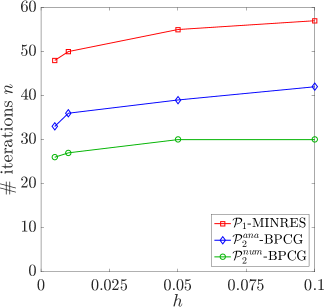
(a)

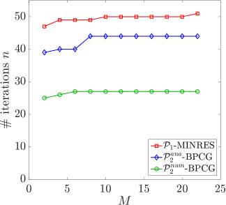
(b)

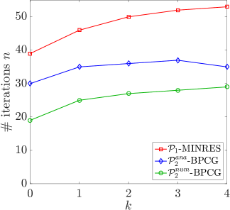
(c)

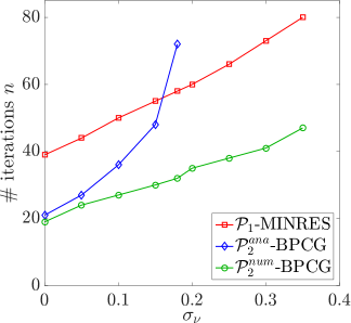
(d)

Figure 1: Iteration counts for $\mathcal{P}_{1}$-MINRES (red), $\mathcal{P}^{ana}_{2}$-BPCG (blue) and $\mathcal{P}^{num}_{2}$-BPCG (green) using different values of the mesh size $h$ (top left), the KLE truncation index $M$ (top right), the degree of the polynomial chaos $k$ (bottom left) and the standard deviation $\sigma_{\nu}$ (bottom right).

The influence of the KLE truncation index $M$ on the convergence of the iterative solvers is displayed in the top right plot of Fig. 1. When increasing $M$, the iteration counts grow slightly up to a certain threshold and then basically stay constant for all three solvers. Asymptotic independence of $M$ thus occurs as predicted. $\mathcal{P}_{1}$-MINRES again has the highest iteration counts followed by $\mathcal{P}^{ana}_{2}$-BPCG and $\mathcal{P}^{num}_{2}$-BPCG.

In Fig. 1, iteration counts for different values of the chaos degree $k$ are displayed on the bottom left. For almost all considered chaos degrees, the three solvers exhibit a slight growth in iteration counts with increasing $k$. For $\mathcal{P}_{1}$-MINRES and $\mathcal{P}^{num}_{2}$-BPCG, this behavior can be observed up to the considered order where for $\mathcal{P}^{ana}_{2}$-BPCG, the iteration counts decrease at the end. The theory did not suggest a dependence on $k$, so the asymptotic regime is apparently not reached yet. We can verify this by looking at the eigenvalues of the stochastic Galerkin matrices $G_{m}$, $m=1,\dots,M$, for $k=3$: $\lambda_{\text{max}}(G_{m})=1.4915$, i.e. the eigenvalues do not immediately fill the whole possible range $[-\sqrt{3},\sqrt{3}]$. In fact, for $k=4$ we get the maximum eigenvalue $\lambda_{\text{max}}(G_{m})=1.570$, which means that increasing the degree of the polynomial chaos leads to new, larger eigenvalues, thereby increasing the iteration count. We suspect that the decrease in iteration counts for $\mathcal{P}^{ana}_{2}$-BPCG has the same cause: For increasing $k$, the analytical scaling improves as it relies on the theoretical bound $\pm\sqrt{3}$.

Figure 1 (bottom right) contains results for different values of the standard deviation $\sigma_{\nu}$. We observe that the iteration counts of all three methods noticeably increase with $\sigma_{\nu}$. This is due to the fact that $\sigma_{\nu}$ directly influences the bounds in the Lemmas 7.1 and 7.3. For the analytically scaled $\mathcal{P}^{ana}_{2}$-BPCG, this influence is particularly pronounced and the algorithm converges merely up to $\sigma_{\nu}=0.18$. This is because the scaling factor $\hat{\delta}$ in Lemma 7.1 contains the term $\underline{\nu}_{0}-\sqrt{3}\,\sigma_{\nu}\,\chi$ which is also the lower bound for the viscosity in Eq. 3.3. In the numerical examples, this term becomes negative for $\sigma_{\nu}>0.18$. Consequently, we can not theoretically guarantee well-posedness of the discrete problem for $\sigma_{\nu}>0.18$ as assumption Eq. 3.4 no longer holds. Still, computing $\lambda_{\text{min}}(\widetilde{\mathcal{A}}_{\text{mg}}^{-1}\mathcal{A})$ numerically showed that the discrete problem is well-posed up to $\sigma_{\nu}\approx 0.35$, independent of the chaos degree. Consequently, we need a lower bound tighter than the one in Eq. 3.3 to make $\mathcal{P}^{ana}_{2}$-BPCG work for $\sigma>0.18$. Yet, for moderate values of $\sigma_{\nu}$, $\mathcal{P}_{1}$-MINRES needs the most iterations, followed by $\mathcal{P}^{ana}_{2}$-BPCG and $\mathcal{P}^{num}_{2}$-BPCG.

10 Conclusion

Based on the SGFE discretization of the Stokes model with random viscosity, we have investigated the efficient solution of the resulting system of equations by means of two suitable preconditioned iterative methods. We have linked the convergence behavior of the solvers to the eigenvalue bounds of the respective relevant sub-matrices. Because the eigenvalue bounds of $\mathcal{P}_{1}^{-1}\mathcal{C}$ and $P_{2}^{-1}\mathcal{C}$ depend on the same parameters, we expect the iteration counts of $\mathcal{P}_{1}$-MINRES and the $\mathcal{P}_{2}$-BPCG methods to depend on these parameters, too. This has been confirmed by numerical experiments. In particular, we have observed the following:

• The mesh size does not have a significant influence on the iteration counts. This is in line with the predictions and results from the use of the spectrally equivalent FE preconditioners.

• The iteration numbers are asymptotically independent of the KLE truncation index. This is an effect of the conditions imposed on the parametrized random viscosity.

• There is a slight increase of iteration counts when the discretization of the random parameter domain is refined. This has been explained by the observation that the eigenvalues do not immediately occupy the whole predicted interval, but fill it steadily as the chaos degree grows. Still, as the uniform random variables are bounded and appear linearly in the input, the condition of the SG matrices is bounded independently of the polynomial chaos degree.

• The condition of the problem critically depends on the variance of the data in relation to its expectation. If the variance becomes too large, the problem even becomes ill-posed. This is reflected by the fact that the convergence deteriorates as the variance increases.

The preconditioner used in the BPCG method contains a scaling to ensure positive definiteness of the matrix $\mathcal{H}$ and $\mathcal{H}$-positive definiteness of the preconditioned system matrix $\mathcal{P}_{2}^{-1}\mathcal{C}$. The optimal scaling parameter is given by the minimum eigenvalue of the preconditioned SGFE Laplacian, as confirmed by the numerical experiments. Still, the numerical costs associated with this eigenvalue problem are prohibitive. We have derived an analytical value for the scaling based on knowledge of the parametrized random input. Numerical tests performed with this value resulted in a reduction of the iteration counts by up to a factor of about 1.5 compared to the reference preconditioned MINRES. The only regime where the analytically scaled BPCG performed worse is close to the analytically derived limit of positivity of the viscosity. We also used the BPCG method with a numerically computed scaling. This approach converged faster than the analytically scaled solver and resulted in a reduction of iteration counts by up to a factor of 2 compared to the preconditioned MINRES method.

Concerning the eigenvalue analysis and the numerical tests, we summarize that the BPCG solver with block triangular preconditioner has the same qualitative properties as block diagonal preconditioned MINRES. When a proper scaling parameter is available, the use of a BPCG solver can result in a noticeable reduction of iteration counts compared to the application of the parameter-free MINRES method with block diagonal preconditioner. At the same time, applying the block triangular preconditioner is only marginally more expensive.

References

- [1] S. F. Ashby, T. A. Manteuffel, and P. E. Saylor, A taxonomy for conjugate gradient methods, SIAM J. Numer. Anal., 27 (1990), pp. 1542–1568, https://doi.org/10.1137/0727091.
- [2] O. Axelsson and M. Neytcheva, Preconditioning methods for linear systems arising in constrained optimization problems, Numer. Lin. Alg. Appl., 10 (2003), pp. 3–31, https://doi.org/10.1002/nla.310.
- [3] I. Babuška, F. Nobile, and R. Tempone, A stochastic collocation method for elliptic partial differential equations with random input data, SIAM J. Numer. Anal., 45 (2007), pp. 1005–1034, https://doi.org/10.1137/050645142.
- [4] I. Babuška, R. Tempone, and G. E. Zouraris, Galerkin finite element approximations of stochastic elliptic partial differential equations, SIAM J. Numer. Anal., 42 (2004), pp. 800–825, https://doi.org/10.1137/S0036142902418680.
- [5] M. Benzi, G. H. Golub, and J. Liesen, Numerical solution of saddle point problems, Acta Numer., 14 (2005), pp. 1–137, https://doi.org/10.1017/S0962492904000212.
- [6] A. Bespalov, C. E. Powell, and D. Silvester, A priori error analysis of stochastic Galerkin mixed approximations of elliptic PDEs with random data, SIAM J. Numer. Anal., 50 (2012), pp. 2039–2063, https://doi.org/10.1137/110854898.
- [7] A. Bespalov and D. Silvester, Efficient adaptive stochastic Galerkin methods for parametric operator equations, SIAM J. Sci. Comput., 38 (2016), pp. A2118–A2140, https://doi.org/10.1137/15M1027048.
- [8] J. H. Bramble and J. E. Pasciak, A preconditioning technique for indefinite systems resulting from mixed approximations of elliptic problems, Math. Comp., 50 (1988), pp. 1–17, https://doi.org/10.1090/S0025-5718-1988-0917816-8.
- [9] F. Brezzi and M. Fortin, Mixed and Hybrid Finite Element Methods, Springer, New York, 1991.
- [10] M. Eigel, C. J. Gittelson, C. Schwab, and E. Zander, Adaptive stochastic Galerkin FEM, Comput. Methods Appl. Mech. Engrg., 270 (2014), pp. 247–269, https://doi.org/10.1016/j.cma.2013.11.015.
- [11] H. C. Elman, A. Ramage, and D. J. Silvester, IFISS: a computational laboratory for investigating incompressible flow problems, SIAM Rev., 56 (2014), pp. 261–273, https://doi.org/10.1137/120891393.
- [12] H. C. Elman, D. J. Silvester, and A. J. Wathen, Finite Elements and Fast Iterative Solvers: with Applications in Incompressible Fluid Dynamics, Oxford Univ. Press, Oxford, 2nd ed., 2014.
- [13] O. G. Ernst, C. E. Powell, D. J. Silvester, and E. Ullmann, Efficient solvers for a linear stochastic Galerkin mixed formulation of diffusion problems with random data, SIAM J. Sci. Comput., 31 (2009), pp. 1424–1447, https://doi.org/10.1137/070705817.
- [14] V. Faber and T. Manteuffel, Necessary and sufficient conditions for the existence of a conjugate gradient method, SIAM J. Numer. Anal., 21 (1984), pp. 352–362, https://doi.org/10.1137/0721026.
- [15] R. G. Ghanem and P. D. Spanos, Stochastic Finite Elements: A Spectral Approach, Springer, New York, 1991.
- [16] M. D. Gunzburger, C. G. Webster, and G. Zhang, Stochastic finite element methods for partial differential equations with random input data, Acta Numer., 23 (2014), pp. 521–650, https://doi.org/10.1017/S0962492914000075.
- [17] W. Hackbusch, Iterative Solution of Large Sparse Systems of Equations, Springer, New York, 1994.
- [18] V. John, Finite Element Methods for Incompressible Flow Problems, Springer, Cham, Switzerland, 2016.
- [19] G. J. Lord, C. E. Powell, and T. Shardlow, An Introduction to Computational Stochastic PDEs, Cambridge University Press, New York, 2014.
- [20] A. W. Marshall and I. Olkin, Inequalities: Theory of Majorization and Its Applications, Academic Press, New York, 1st ed., 1979.
- [21] C. Müller, Iterative solvers for stochastic Galerkin discretizations of Stokes flow with random data, PhD thesis, TU Darmstadt, 2018.
- [22] C. Müller, S. Ullmann, and J. Lang, A Bramble-Pasciak conjugate gradient method for discrete Stokes problems with lognormal random viscosity, in Recent Advances in Computational Engineering, ICCE 2017, M. Schäfer, M. Behr, M. Mehl, and B. Wohlmuth, eds., vol. 124 of Lect. Notes Comput. Sci. Eng., Cham, 2018, Springer, https://doi.org/10.1007/978-3-319-93891-2_5.
- [23] B. Oksendal, Stochastic Differential Equations: An Introduction With Applications, Springer, Berlin, 5th ed., 1998.
- [24] C. C. Paige and M. A. Saunders, Solution of sparse indefinite systems of linear equations, SIAM J. Numer. Anal., 12 (1975), pp. 617–629, https://doi.org/10.1137/0712047.
- [25] J. Peters, V. Reichelt, and A. Reusken, Fast iterative solvers for discrete Stokes equations, SIAM J. Sci. Comput., 27 (2005), pp. 646–666, https://doi.org/10.1137/040606028.
- [26] C. E. Powell and H. C. Elman, Block-diagonal preconditioning for spectral stochastic finite-element systems, IMA J. Numer. Anal., 29 (2009), pp. 350–375, https://doi.org/10.1093/imanum/drn014.
- [27] C. E. Powell and D. J. Silvester, Preconditioning steady-state Navier–Stokes equations with random data, SIAM J. Sci. Comput., 34 (2012), pp. A2482–A2506, https://doi.org/10.1137/120870578.
- [28] I. Pultarová, Adaptive algorithm for stochastic Galerkin method, Appl. Math., 60 (2015), pp. 551–571, https://doi.org/10.1007/s10492-015-0111-9.
- [29] E. Rosseel and S. Vandewalle, Iterative solvers for the stochastic finite element method, SIAM J. Sci. Comput., 32 (2010), pp. 372–397, https://doi.org/10.1137/080727026.
- [30] Y. Saad and M. H. Schultz, GMRES: A generalized minimal residual algorithm for solving nonsymmetric linear systems, SIAM J. Sci. and Stat. Comput., 7 (1986), pp. 856–869, https://doi.org/10.1137/0907058.
- [31] D. Silvester and A. Wathen, Fast iterative solution of stabilised Stokes systems part II: using general block preconditioners, SIAM J. Numer. Anal., 31 (1994), pp. 1352–1367, https://doi.org/10.1137/0731070.
- [32] E. Ullmann, A Kronecker product preconditioner for stochastic Galerkin finite element discretizations, SIAM J. Sci. Comput., 32 (2010), pp. 923–946, https://doi.org/10.1137/080742853.
- [33] S. Ullmann, Triangular Taylor Hood finite elements, 2017, https://www.mathworks.com/matlabcentral/fileexchange/49169. Version 1.4.
- [34] H. A. van der Vorst, Bi-CGSTAB: A fast and smoothly converging variant of Bi-CG for the solution of nonsymmetric linear systems, SIAM J. Sci. and Stat. Comput., 13 (1992), pp. 631–644, https://doi.org/10.1137/0913035.
- [35] A. J. Wathen, On relaxation of Jacobi iteration for consistent and generalized mass matrices, Commun. Appl. Numer. Methods, 7 (1991), pp. 93–102, https://doi.org/10.1002/cnm.1630070203.
- [36] D. Xiu and G. E. Karniadakis, The Wiener–Askey polynomial chaos for stochastic differential equations, SIAM J. Sci. Comput., 24 (2002), pp. 619–644, https://doi.org/10.1137/S1064827501387826.
- [37] W. Zulehner, Analysis of iterative methods for saddle point problems: a unified approach, Math. Comp., 71 (2001), pp. 479–505, http://www.jstor.org/stable/2698830.