Scaling Behavior in the 3D Random Field $XY$ Model

Abstract

We have performed studies of the 3D random field $XY$ model on $L\times L\times L$ simple cubic lattices with periodic boundary conditions, with a random field strength of $h_{r}$ = 1.875, for $L=64$ and $L=96$, using a parallelized Monte Carlo algorithm. We present results for the angle-averaged magnetic structure factor, $S(k)$ at $T=1.00$, which appears to be the temperature at which small jumps in the magnetization per spin and the energy per spin occur. The results indicate the existence of an approximately logarithmic divergence of $S(k)$ as $k\to 0$. This suggests that the lower critical dimension for long range order in this model is three.

I Introduction

The behavior of the three-dimensional (3D) random-field $XY$ model (RFXYM) at low temperatures and weak to moderate random field strengths continues to be controversial. A detailed calculation by LarkinLar70 showed that, in the limit that the number of spin components, $n$, becomes infinite, the ferromagnetic phase becomes unstable when the spatial dimension of the lattice is less than or equal to four, $d\leq 4$. Dimensional reduction argumentsIM75 ; AIM76 appeared to show that the long-range order is unstable for $d\leq 4$ for any finite $n\geq 2$. However, there are several reasons for questioning whether dimensional reduction can be trusted for $XY$, i.e. $n=2$, spins.

Some time ago, Monte Carlo calculationsGH96 ; Fis97 showed that there was a line in the temperature vs. random-field plane of the phase diagram of the three-dimensional (3D) random-field $XY$ model (RFXYM), at which the magnetic structure factor becomes large as the wave-number $k$ becomes small. Additional calculationsFis07 indicated that there appeared to be small jumps in the magnetization and the energy of $L=64$ lattices at a random field strength of $h_{r}=2.0$, at a temperature somewhat below $T=1.0$. Further calculationsFis10 showing similar behavior for other values of the random field strength were also performed. If such behavior persists for larger values of $L$, this would demonstrate that there is a ferromagnetic phase at weak to moderate random fields and low temperatures for this model.

Since there have been substantial improvements in computing hardware and software over the last ten years, the author felt it worthwhile to conduct a new Monte Carlo study of this model using parallel processing. The results of that study for $L=64$ and $L=96$ will be presented here. The extension of the methods used here to $L=128$ lattices is currently in progress.

II The Model

For fixed-length classical spins the Hamiltonian of the RFXYM is

$$H~{}=~{}-J\sum_{\langle ij\rangle}\cos(\phi_{i}-\phi_{j})~{}-~{}h_{r}\sum_{i}\cos(\phi_{i}-\theta_{i})\,.$$ (1)

Each $\phi_{i}$ is a dynamical variable which takes on values between 0 and $2\pi$. The $\langle ij\rangle$ indicates here a sum over nearest neighbors on a simple cubic lattice of size $L\times L\times L$. We choose each $\theta_{i}$ to be an independent identically distributed quenched random variable, with the probability distribution

$$P(\theta_{i})~{}=~{}1/2\pi\,$$ (2)

for $\theta_{i}$ between 0 and $2\pi$. We set the exchange constant to $J=1$, with no loss of generality. This Hamiltonian is closely related to models of vortex lattices and charge density waves.GH96 ; Fis97

LarkinLar70 studied a model for a vortex lattice in a superconductor. His model replaces the spin-exchange term of the Hamiltonian with a harmonic potential, so that each $\phi_{i}$ is no longer restricted to lie in a compact interval. He argued that for any non-zero value of $h_{r}$ this model has no ferromagnetic phase on a lattice whose dimension $d$ is less than or equal to four. The Larkin approximation is equivalent to a model for which the number of spin components, $n$, is sent to infinity. A more intuitive derivation of this result was given by Imry and Ma,IM75 who assumed that the increase in the energy of an $L^{d}$ lattice when the order parameter is twisted at a boundary scales as $L^{d-2}$ for all $n>1$, just as it would for $h_{r}=0$. Using this assumption, they argued that when $d\leq 4$ there is a length $\lambda$, now called the Imry-Ma length, at which the energy which can be gained by aligning a spin domain with its local random field exceeds the energy cost of forming a domain wall. From this they claimed that the magnetization would decay to zero when the system size, $L$, exceeds $\lambda$.

Within a perturbative $\epsilon$-expansion one finds the phenomenon of “dimensional reduction”. The critical exponents of any $d$-dimensional $O(n)$ random-field model appear to be identical to those of an ordinary $O(n)$ model of dimension $d-2$. For the $n=1$ (RFIM) case, this was soon shown rigorously to be incorrect for $d<4$.Imb84 ; BK87 More recently, extensive numerical results for the Ising case have been obtained for $d=4$ and $d=5$.FMPS17a ; FMPS17b They determined that dimensional reduction is ruled out numerically in the Ising case for $d=4$, but not for $d=5$.FMPS17c

Because translation invariance is broken for any non-zero $h_{r}$, it seems quite implausible to the current author that the twist energy for Eqn. (1) scales as $L^{d-2}$, even though this is correct to all orders in perturbation theory. An alternative derivation by Aizenman and Wehr,AW89 ; AW90 which claims to be mathematically rigorous, also makes an assumption equivalent to translation invariance. Although the average over the probability distribution of random fields restores translation invariance, one must take the infinite volume limit first. It is not correct to interchange the infinite volume limit with the average over random fields. This problem of the interchange of limits is equivalent to the existence of replica symmetry breaking. The existence of replica symmetry breaking in random field models was first shown by Mezard and Young,MY92 about two years after the work of Aizenman and Wehr. Mezard and Young emphasized the Ising case, and the fact that this applies for all finite $n$ seems to have been overlooked by many people for a number of years. A functional renormalization group calculation going to two-loop order was performed by Tissier and Tarjus,TT06 and independently by Le Doussal and Wiese.LW06 They found that there was a stable critical fixed point of the renormalization group for some range of $d$ below four dimensions in the $n=2$ random field case. However, it is not clear from their calculation what the nature of the low-temperature phase is, or whether this fixed point is stable down to $d=3$. Tarjus and TissierTT08 later presented an improved version of this calculation, which explains more explicitly why dimensional reduction fails for the $n=2$ case when $d\leq 4$.

III Structure factor

The magnetic structure factor, $S(\vec{\bf k})=\langle|\vec{\bf M}(\vec{\bf k})|^{2}\rangle$, for $XY$ spins is

$$S(\vec{\bf k})~{}=~{}L^{-3}\sum_{i,j}\cos(\vec{\bf k}\cdot\vec{\bf r}_{ij})\langle\cos(\phi_{i}-\phi_{j})\rangle\,,$$ (3)

where $\vec{\bf r}_{ij}$ is the vector on the lattice which starts at site $i$ and ends at site $j$, and here the angle brackets denote a thermal average. For a random field model, unlike a random bond model, the longitudinal part of the magnetic susceptibility, $\chi$, which is given by

$$T\chi(\vec{\bf k})~{}=~{}1-M^{2}~{}+~{}L^{-3}\sum_{i\neq j}\cos(\vec{\bf k}\cdot\vec{\bf r}_{ij})(\langle\cos(\phi_{i}-\phi_{j})\rangle~{}-~{}Q_{ij})\,,$$ (4)

is not the same as $S$ even above $T_{c}$. For $XY$ spins,

$$Q_{ij}~{}=~{}\langle\cos(\phi_{i})\rangle\langle\cos(\phi_{j})\rangle~{}+~{}\langle\sin(\phi_{i})\rangle\langle\sin(\phi_{j})\rangle\,,$$ (5)

and

$$M^{2}~{}=~{}L^{-3}\sum_{i}Q_{ii}~{}=~{}L^{-3}\sum_{i}\langle\cos(\phi_{i})\rangle^{2}~{}+~{}\langle\sin(\phi_{i})\rangle^{2}\,.$$ (6)

When there is a ferromagnetic phase transition, $S(\vec{\bf k}=0)$ has a stronger divergence than $\chi(\vec{\bf k}=0)$.

The scalar quantity $\langle M^{2}\rangle$, when averaged over a set of random samples of the random fields, is a well-defined function of the lattice size $L$ for finite lattices. With high probability, it will approach its large $L$ limit smoothly as $L$ increases. The vector $\vec{\bf M}$, on the other hand, is not really a well-behaved function of $L$ for an $XY$ model in a random field. Knowing the local direction in which $\vec{\bf M}$ is pointing, averaged over some small part of the lattice, may not give us a strong constraint on what $\langle\vec{\bf M}\rangle$ for the entire lattice will be. When we look at the behavior for all $k$, instead of merely looking at $k=0$, we get a much better idea of what is really happening.

IV Numerical results for $S(k)$

In this work, we will present results for the average over angles of $S(\vec{\bf k})$, which we write as $S(k)$. The data were obtained from $L\times L\times L$ simple cubic lattices with $L=64$ and $L=96$ using periodic boundary conditions. The calculations were done using a clock model which has 8 equally spaced dynamical states at each site. In addition, there is a static random phase at each site which was chosen to be $0,\pi/12$ or $\pi/6$ with equal probability. It has been known for some time that a model of this type, without the random-field term, is in the universality class of the pure $XY$ model under most conditions, even if the number of dynamical states of each spin is only 3.Fis92 Under conditions of very low temperature, this model may undergo an incommensurate-to-commensurate type of charge-density wave phase transition. Thus it is expected that, when we include the random-field term, the model will behave essentially as a random-field $XY$ model, as long as we do not attempt to work at very low temperature.Fis97

The strength of the random field for which data were obtained is $h_{r}$ = 1.875. This value was chosen in order to make the value of $T_{c}$ close to 1.00. The direction of the random field at site $i$, $\theta_{i}$, was chosen randomly from the set of the 24th roots of unity, independently at each site. Since $\theta_{i}$ has 24 possible values, our past experience with models of this type indicates that there is no possibility that the discretization will affect the behavior near $T=1.00$ in an observable way.

The computer program uses three independent pseudorandom number generators: one for choosing the values of the $\theta_{i}$, one for setting the static random phases, and a third one for the Monte Carlo spin flips, which are performed by a single-spin-flip heat-bath algorithm. The pseudorandom number generator used for the Monte Carlo spin flips was the library function $random\_number$, supplied by the Intel Fortran compiler, which is suitable for parallel computation. The spin-flip subroutine was parallelized using OpenMP, by taking advantage of the fact that the simple cubic lattice is two colorable. It was run on Intel multicore processors of the Bridges Regular Memory machine at the Pittsburgh Supercomputer Center. The code was checked by setting $h_{r}=0$, and seeing that the known behavior of the pure ferromagnetic 3D XY model was reproduced correctly.

24 different realizations of the random fields $\theta_{i}$ were studied for $L=64$, and another 24 samples were studied for $L=96$. Each lattice was started off in a random spin state at $T=2.25$, above the $T_{c}$ for the pure model, and cooled slowly to $T=1.00$. At $T=1.00$, the sample was relaxed until an apparent equilibrium was reached over an appropriate time scale. For $L=64$ this time scale was 163,840 Monte Carlo steps per spin (MCS), and for $L=96$ this was increased to at least 655,360 MCS. Some $L=96$ samples required relaxation for up to three times longer.

After each sample was relaxed at $T=1.00$, a sequence of 8 equilibrated spin states obtained at intervals of 20,480 MCS for $L=64$ or 40,960 MCS for $L=96$ was Fourier transformed to calculate $S(\vec{bfk})$, and then averaged over the sequence of 8 spin states. The data were then binned according to the value of $k^{2}$, to give the angle-averaged $S(k)$. Finally, an average over the 24 samples was performed for each $L$. The average magnetization per spin at $T=1.00$ of these slowly cooled samples was $0.139\pm 0.011$ for $L=64$, and $0.080\pm 0.011$ for $L=96$.

Data were also obtained for the same sets of samples using ordered initial states and warming to $T=1.00$. At least two, and sometimes more initial ordered states were used for each sample. The initial magnetization directions used were chosen to be close to the direction of the magnetization of the slowly cooled sample with the same set of random fields. This type of initial state was chosen because it was found in the earlier workFis07 that this is the way to find the lowest energy minima in the phase space. The data from the initial condition which gave the lowest average energy for a given sample was then selected for further analysis and comparison with the slowly cooled state data from that sample. The relaxation procedure at $T=1.00$ for the warmed states was the same one used for the cooled states, and the calculation of $S(k)$ proceeded in the same way. The average magnetization per spin of these selected warmed states was $0.239\pm 0.010$ for $L=64$, and $0.157\pm 0.011$ for $L=96$.

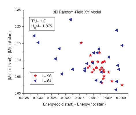
Figure 1: (color online) Jump in the magnetization vs. jump in the energy for $L=64$ and $L=96$ simple cubic lattices with $h_{r}=1.875$ at $T=1.00$. States with hot start and ordered start initial conditions are compared for each sample.

In order to compare the $L=64$ data with the $L=96$ data, the energy per spin difference and the magnetization per spin difference between the cooled state and the warmed state at $T=1.00$ were computed for each sample. The results are shown in a scatter plot in Fig. 1. We see that the distributions do not show any significant correlation between the energy difference and the magnetization difference for the $L=64$ samples. For the $L=96$ samples there is a weak tendency for the size of the jump in the magnetization to be correlated with the size of the jump in the energy. The distribution is rather broad for $L=64$, and significantly narrower for $L=96$.

The center of the $L=64$ distribution is at $\delta|M|=0.100\pm 0.011$ and $\delta E=-0.00113\pm 0.00019$, while the center of the $L=96$ distribution is at $\delta|M|=0.077\pm 0.006$ and $\delta E=-0.00078\pm 0.00006$. The conjecture that $\delta|M|$ and $\delta E$ will scale to zeroFis07 as $L\to\infty$ is consistent with these data. There is some indication that $\delta|M|$ scales more slowly than $\delta E$, but more data are needed before any quantitative estimate of the rates of convergence of these parameters can be made. The author is planning to make such estimates when data for $L=128$ samples become available.

The average specific heat of the $L=64$ samples at $T=1.00$ is $0.7797\pm 0.0019$ for the cooled samples, and $0.7815\pm 0.0028$ for the heated samples. The corresponding numbers for $L=96$ are $0.7802\pm 0.0028$ and $0.7854\pm 0.0026$. The fact that the specific heat of the cooled samples is lower than the specific heat of the somewhat more magnetized heated samples is expected. The fact that the difference between them is very small means that there is not much energy associated with the disappearance of the magnetic long-range order. The fact that the jump in the specific heat seems to be slightly larger for $L=96$ than for $L=64$ is normal for a weakly first-order phase transition. The fact that the jump is so small also means that we are not looking at a normal second order phase transition.

The uncertainty in our estimate of the $T_{c}$, the temperature of the phase transition, is about an order of magnitude less than the extrapolated shift in temperature which would be needed to make the jump in energy between the heated samples and the cooled samples disappear. However, the free-energy minimum of a cold-start sample actually becomes clearly unstable at a temperature a few percent higher than $T=1.00$.

Now we turn to the data for the structure factor. The average $S(k)$ for the 24 $L=96$ samples at $T=1.00$ is shown in Fig. 2. $S(k)$ is computed separately for the heated sample data and the cooled sample data, but it is difficult to see any difference between them. These data are very similar to the earlier dataFis07 for $h_{r}=2$ at $T=0.875$. The change in the slope of the data points now occurs near $k=0.11$ instead of $k=0.14$, but this is about what is expected from using the somewhat lower value of $h_{r}$. From this log-log plot, it is not clear how to extrapolate the data to small $k$.

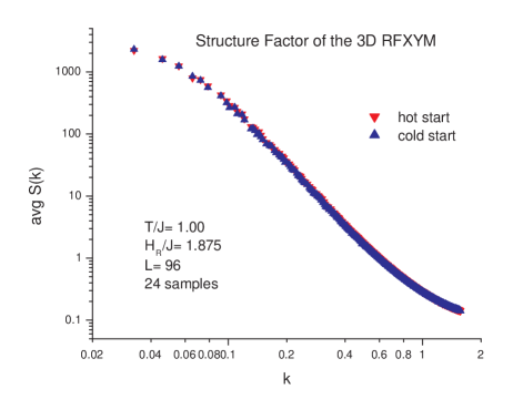
Figure 2: (color online) Angle-averaged structure factor vs. $k$ for $96\times 96\times 96$ lattices with $h_{r}=1.875$ at temperature T = 1.00. Both the $x$-axis and the $y$-axis are scaled logarithmically. One $\sigma$ statistical errors are approximately the size of the plotting symbols.

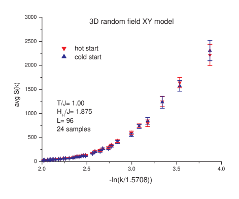
Figure 3: (color online) Angle-averaged structure factor vs. (- ln(k/1.5708)) for $96\times 96\times 96$ lattices with $h_{r}=1.875$ at temperature T = 1.00. One $\sigma$ statistical errors are shown.

To clarify the behavior at small $k$, we replot the same $L=96$ data for the structure factor on a linear scale in Fig. 3. The scaling for the $x$-axis is chosen so that the edge of the Brillouin zone would be at $x=0$, but only the small-$k$ part of the data are shown on the graph. From Fig. 3 it is clear that we have no evidence for a finite correlation length at $L=96$. However, these data also appear to rule out the possibility that $S(k)$ behaves like $k^{4-\bar{\eta}}$ with $1<\bar{\eta}\leq 2$ as $k\to 0$, which would be required for hyperscaling to hold.

A divergence of $S(k)$ as $k\to 0$ like $\ln(k)$, or some power of $\ln(k)$, is a strong indicator that the lower critical dimension of the RFXYM is exactly equal to three. The author is not aware of another example of this type of behavior in a model with quenched random disorder, and much remains to be learned. It would be very exciting if similar behavior was observed by doing experiments on physical systems which are believed to be in the universality class of this model.

V Discussion

It is straightforward to calculate the interaction energy of the spins with the random field. We merely need to calculate the value of the second sum in the Hamiltonian as a function of the temperature. When this is done at $h_{r}=1.875$, it turns out that the value of the random-field energy has a maximum at about $T=1.75$ Below that temperature, the ferromagnetic bonds become increasingly successful in pulling the directions of the local spins away from the directions of their local random fields. Of course, there is nothing magic about $T=1.75$. The temperature at which the maximum value in the random-field energy will occur will be a function of the value of $h_{r}$. This effect is not accounted for in the Imry-Ma argument.

Finding that $S(k)$ diverges at low temperatures in the RFXYM as $k\to 0$ is not surprising. This behavior follows from the results of AharonyAha78 for models which have a probability distribution for the random fields which is not isotropic. According to Aharony’s calculation, if this distribution is even slightly anisotropic, then we should see a crossover to RFIM behavior. We knowImb84 ; BK87 that in $d=3$ the RFIM is ferromagnetic at low temperature if the random fields are not very strong. The instability to even a small anisotropy in the random field distribution should induce a diverging response in $S(k)$ as $k\to 0$ for the RFXYM in $d=3$. A similar effect in a related, but somewhat different, model was found by Minchau and Pelcovits.MP85 .

There has been no attempt in this work to equilibrate samples at temperatures below the apparent critical temperature. Therefore we have no data which directly address the question of whether the RFXYM shows true ferromagnetism in $d=3$. If we assume that the average $|M|$ of finite samples is subextensive, i.e. the net magnetic moment grows more slowly than $L^{3}$ as $L\to\infty$, then it would follow from the above argument that there should not be any divergence of $S(k)$ for $k\to 0$ in $d=3$ in the cases $n\geq 3$. If this were the case, then the behavior of random field $O(n)$ models in $d=3$ would be remarkably parallel to the case of the ordinary $O(n)$ ferromagnets in $d=2$. One might hope to find a relatively simple reason for such an effect.

About five years ago, numerical studies of the RFXYM were performed by Garanin. Chudnovsky and Proctor.GCP13 These authors were interested in studying lattices of very large $L$. Such lattices were much too large for the simulations to be able to reach a thermal equilibrium, and they did not use any Boltzmann factors in their dynamics. Thus the results are some kind of simulated annealing, and it is not clear what the meaning of their end states is. The work being reported here always used Boltzmann factors to relax the state of the lattice. It is not possible to make any quantitative comparison, because they only study low energy states, and give no results for the behavior at the phase transition. In further work,PGC14 these authors extend their methods to models with other numbers of spin components. They claim that the 3D $n=3$ spin model in a random field of $h_{r}=1.5$ also has a stable ferromagnetic phase at low temperature, but do not give an estimate of $T_{c}$. They also claim that for 2D, the RFXYM has a ferromagnetic state for $h_{r}=0.5$, which is surely incorrect. Therefore the reliability of their methods is highly questionable. The functional renormalization group calculationsTT06 ; LW06 ; TT08 do not give any support for the existence of a ferromagnetic phase for the $n=3$ random field case for $d\leq 4$.

There is another model which is more similar to the random-field $XY$ model than the random-field Ising model is. That model is the 3-state Potts model in a random field (RFPM). In the absence of the random-field term, a 3D 3-state Potts model has a first-order phase transition, with a substantial latent heat at $T_{c}$. In 1989, two groups presented independent arguments showing that models like this should no longer have a latent heat when the random-field term is added to the Hamiltonian. Aizenman and WehrAW89 proved that the latent heat must vanish in the limit $L\to\infty$. Hui and BerkerHB89 argued that the vanishing of the latent heat implied that a critical fixed point should exist. This author does not see, however, why such a fixed point, with its associated divergent correlation length, should generally exist in a model which has no translation symmetry, except in those cases where the randomness is an irrelevant operator.Har74 It is certainly true that there are some cases where such fixed points have been found using $\epsilon$-expansion calculations. Subextensive singularities in the specific heat and the magnetization are completely consistent with the Aizenman-Wehr Theorem.

VI Summary

In this work we have performed Monte Carlo studies of the 3D RFXYM on $L=64$ and $L=96$ simple cubic lattices, with a random field strength of $h_{r}=1.875$. We compare the properties of slowly cooled states and slowly heated states at $T=1.00$, which is our estimate of the temperature at which there appears to be a phase transition. We display results for the change in energy and the change in magnetization at this temperature, as a function of the lattice size. At the phase transition we measure small jumps in the magnetization per spin and the energy per spin. However, it is likely that these jumps are subextensive, meaning that they probably scale to zero as $L\to\infty$. We also compute results for the structure factor, $S(k)$, under these conditions. For $L=96$ the structure factor appears to be have an approximately logarithmic divergence in the small $k$ limit. These characteristics are consistent with the idea that the lower critical dimension of this model is exactly three.

- (1) A. I. Larkin, Zh. Eksp. Teor. Fiz. 58, 1466 (1970) [Sov. Phys. JETP 31, 784 (1970)].
- (2) Y. Imry and S.-K. Ma, Phys. Rev. Lett. 35, 1399 (1975).
- (3) A. Aharony, Y. Imry and S.-K. Ma, Phys. Rev. Lett. 36, 1364 (1976).
- (4) M. J. P. Gingras and D. A. Huse, Phys. Rev. B 53, 15193 (1996).
- (5) R. Fisch, Phys. Rev. B 55, 8211 (1997).
- (6) R. Fisch, Phys. Rev. B 76, 214435 (2007).
- (7) R. Fisch, arXiv:1001.3397.
- (8) J. Z. Imbrie, Phys. Rev. Lett. 53, 1747 (1984).
- (9) J. Bricmont and A. Kupiainen, Phys. Rev. Lett. 59, 1829 (1987).
- (10) N. G. Fytas, V. Martin-Mayor, M. Picco and N. Sourlas, J. Stat.Mech. 033302 (2017).
- (11) N. G. Fytas, V. Martin-Mayor, M. Picco and N. Sourlas, Phys. Rev. E 95, 042117 (2017).
- (12) N. G. Fytas, V. Martin-Mayor, M. Picco and N. Sourlas, arXiv:1711.09597v3.
- (13) M. Aizenman and J. Wehr, Phys. Rev. Lett. 62, 2503 (1989); erratum: Phys. Rev. Lett. 64, 1311 (1990).
- (14) M. Aizenman and J. Wehr, Commun. Math. Phys. 130, 489 (1990).
- (15) M. Mezard and A. P. Young, Europhys. Lett. 18, 653 (1992).
- (16) M. Tissier and G. Tarjus, Phys. Rev. Lett. 96, 087202 (2006); Phys. Rev B 74, 214419 (2006).
- (17) P. Le Doussal and K. J. Wiese, Phys. Rev. Lett. 96, 197202 (2006).
- (18) M. Tissier and G. Tarjus, Phys. Rev B 78, 024204 (2008).
- (19) R. Fisch, Phys. Rev. B 46, 242 (1992).
- (20) A. Aharony, Phys. Rev. B 18, 3328 (1978).
- (21) B. J. Minchau and R. A. Pelcovits, Phys. Rev. B 32, 3081 (1985).
- (22) D. A. Garanin, E. M. Chudnovsky and T. Proctor, Phys. Rev. B 88, 224418 (2013).
- (23) T. C. Proctor, D. A. Garanin and E. M. Chudnovsky, Phys. Rev. Lett. 112, 097201 (2014).
- (24) K. Hui and A. N. Berker, Phys. Rev. Lett. 62, 2507 (1989).
- (25) A. B. Harris, J. Phys. C 7, 1671 (1974).