On a numerical upper bound for the extended Goldbach conjecture
David Quarel
david.quarel@anu.edu.au
June 2017
A thesis submitted for the degree of Bachelor of Science (Advanced) (Honours)
of the Australian National University
Revised December 2017
![[Uncaptioned image]](/html/1801.01813/assets/x1.png)
Declaration
The work in this thesis is my own except where otherwise stated.
David Quarel
Acknowledgements
I wish to thank my supervisor Tim Trudgian. His advice and weekly meetings provided much needed support whenever I’d get stuck on a problem or become disheartened. I find myself in the most fortunate position of finishing honours in mathematics with the same person as when I started it, way back in 2013 when I took MATH1115.111I still remember the hilarious anecdote in class about cutting a cake “coaxially”.
Having the most engaging lecturer during my first year of undergraduate helped to foster my interest in mathematics, and I’ve yet to see any other lecturer at this university take the time to write letters of congratulations to those that did well in their course.
Abstract
The Goldbach conjecture states that every even number can be decomposed as the sum of two primes. Let denote the number of such prime decompositions for an even . It is known that can be bounded above by
where denotes Chen’s constant. It is conjectured [20] that . In 2004, Wu [54] showed that . We attempted to replicate his work in computing Chen’s constant, and in doing so we provide an improved approximation of the Buchstab function ,
based on work done by Cheer and Goldston [6]. For each interval , they expressed as a Taylor expansion about . We expanded about the point , so was never evaluated more than away from the center of the Taylor expansion, which gave much stronger error bounds.
Issues arose while using this Taylor expansion to compute the required integrals for Chen’s constant, so we proceeded with solving the above differential equation to obtain , and then integrating the result. Although the values that were obtained undershot Wu’s results, we pressed on and refined Wu’s work by discretising his integrals with finer granularity. The improvements to Chen’s constant were negligible (as predicted by Wu). This provides experimental evidence, but not a proof, that were Wu’s integrals computed on smaller intervals in exact form, the improvement to Chen’s constant would be similarly negligible. Thus, any substantial improvement on Chen’s constant likely requires a radically different method to what Wu provided.
Notation and terminology
In the following, usually denote primes.
Notation
-
GRH
Generalised Riemann hypothesis.
-
TGC
Ternary Goldbach conjecture.
-
GC
Goldbach conjecture.
-
FTC
Fundamental theorem of calculus.
-
is an asymptotic upper bound for , that is, there exists constants and such that for all , .
-
is an asymptotic lower bound for , that is, there exists constants and such that for all , . Equivalent to .
-
is an asymptotic tight bound for , that is, . Implies that and .
-
Twin primes constant, §1.10
-
Number of primes less than .
-
Set of all primes .
-
Set of all numbers with at most prime factors. Also denoted for brevity.
-
Sifting function, §2.1.
-
Set of numbers to be sifted by a sieve .
-
-
for some square-free .
-
Characteristic function on a set . Equals 1 if , 0 otherwise.
-
Usually denotes a set of primes.
-
Shorthand for , denotes the main term in an approximation to a sieve.
-
The remainder, or error term, for an approximation to a sieve.
-
Chen’s constant, §1.8.
-
Buchstab’s function, §4.1.
-
Euler–Mascheroni constant.
-
Möbius function.
-
Euler totient function.
-
Linnik–Goldbach constant, §1.9.
-
The cardinality of the set .
-
Greatest common divisor of and . Sometimes denoted if is ambiguous and could refer to an ordered pair.
-
Least common multiple of and .
-
Dirichlet convolution of and , defined as
-
divides , i.e. there exists some such that .
-
does not divide
-
Logarithmic integral,
Chapter 1 History of Goldbach problems
1.1 Origin
One of the oldest and most difficult unsolved problems in mathematics is the
Goldbach conjecture (sometimes called the Strong Goldbach conjecture), which originated during
correspondence between Christian Goldbach
and Leonard Euler in 1742. The Goldbach conjecture states that “Every even integer can be expressed as the sum of two primes” [17].
For example,
Evidently, this decomposition need not be unique. The Goldbach Conjecture has been verified by computer search for all even [12], but the proof for all even integers remains open.***Weakening Goldbach to be true for only sufficiently large is also an open problem. Some of the biggest steps towards solving the Goldbach conjecture include Chen’s theorem [44] and the Ternary Goldbach conjecture [23].
1.2 Properties of
As the Goldbach conjecture has been unsolved for over 250 years, a lot of work has gone into solving weaker statements, usually by weakening the statement that is the sum of two primes. Stronger statements have also been explored. We define as the number of ways can be decomposed into the sum of two primes. The Goldbach conjecture is then equivalent to for all . As grows larger, more primes exist beneath (approximately many, from the prime number theorem) that could be used to construct a sum for . Thus, we expect large numbers to have many prime decompositions. And indeed empirically this seems to be the case.

Below are some examples of prime decompositions of even numbers.
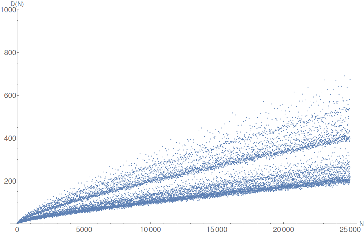
Intuitively, we would expect that as grows large, should likewise grow large. The extended Goldbach conjecture [20] asks how grows asymptotically. As expected, the conjectured formula for grows without bound as increases (Figure 1.2).
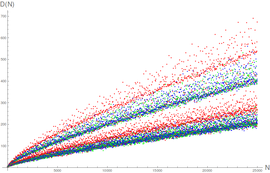
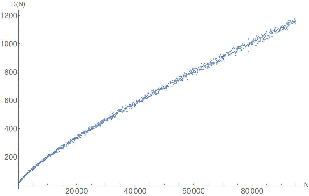
We can see from the plots that the points of cluster into bands, and also shares this property (Figure 1.2). The plot of called “Goldbach’s Comet” [14], which has many interesting properties. We plot , and colour each point either red, green or blue if is 0, 1 or 2 respectively (Figure 1.4). [14]. We can see the bands of colours are visibly separated. If is plotted only for prime multiples of an even number [2], say
the resulting plot is almost a straight line (Figure 1.4).
1.3 Ternary Goldbach conjecture
The Ternary Goldbach conjecture (TGC) states that “every odd integer greater than 5 can be expressed as the sum of three primes”. This statement is directly implied by the Goldbach conjecture, as if every even can be expressed as , where prime, we can express all odd integers greater than 5 as three primes
In 1923, Hardy and Littlewood [20] showed that, under the assumption of the generalised Riemann hypothesis (GRH), the TGC is true for all sufficiently large odd numbers. They also specified how (the number of ways can be decomposed as the sum of three primes) grows asymptotically
| (1.1) |
where
Using the Taylor expansion of and the fact that every term in the sum is positive, we obtain the inequality
Hence by induction, for all non-negative sequences
| (1.2) |
Therefore we may note that must converge, as
We also note that the product over all primes dividing in (1.1) grows slowly compared to the main term, as for all
We have from Mertens’ theorem [10] that
| (1.3) |
Combining this with the following inequality
| (1.4) |
we obtain
which gives an asymptotic lower bound on
This gives a stronger version of the TGC, as it implies that the number of different ways that an odd integer can be decomposed as the sum of three primes can be arbitrarily large. In 1937, Vinogradov improved this result by removing the dependency on GRH [50].
An explicit value for how large needs to be before the TGC holds was found by Borozdin, who showed that is sufficient [16]. In 1997, the TGC was shown to be conditionally true for all odd by Deshouillers et al, [11] under the assumption of GRH. The unconditional TGC was further improved by Liu and Wang [34] in 2002, who showed that Borozdin’s constant can be reduced to . Thus, in principle, all that was needed to prove the TGC was to check that it held for all . Given that the number of particles in the universe , no improvements to computational power would likely help. Further mathematical work was necessary.
1.4 Extended Goldbach conjecture
Hardy and Littlewood’s paper [20] discuss how one can directly obtain an asymptotic formula (conditional on GRH) for the numbers of ways even can be decomposed into the sum of four primes. Let be the number of such ways.
| (1.5) |
where
The asymptotic formulae for and are very similar (checking convergence and the long term behaviour of is the same proof as for ). Hardy–Littlewood claim that one can easily generalise their work to obtain an asymptotic formula for for . However, for , the results do not easily generalise:
“It does not fail in principle, for it leads to a definite result which appears to be correct; but we cannot overcome the difficulties of the proof…”[20, p. 32]
The following asymptotic formula for was thus conjectured [20]
| (1.6) |
where
Now denotes the twin primes constant (see 1.10), and each term in the infinite product in is greater than 1. Thus, , which provides an asymptotic lower bound of
| (1.7) |
Hence, (1.6) implies the Goldbach conjecture (for large ), which should indicate the difficulty of the problem.
There has been progress in using (1.6) as a way to construct an upper bound for , by seeking the smallest values of (hereafter referred to as Chen’s constant) such that
| (1.8) |
Upper bounds for have been improved over the years, but recent improvements have been small222We remind the reader than is conjectured to be 2. (see Table 1.1). Recent values have been obtained by various sieve theory methods by constructing large sets of weighted inequalities (the one in Wu’s paper has 21 terms!). However, the reductions in are minuscule. One would suspect that any further improvements would require a radically new method, instead of complicated inequalities with more terms.
1.5 The Linnik–Goldbach problem
The Linnik–Goldbach problem [41] is another weaker form of the GC, which asks for the smallest values of such that for all sufficient large even ,
| (1.9) |
That is, we can express as the sum of two primes and at most powers of two (we refer to as the Linnik–Goldbach constant). In 1953, Linnik [30] proved that there exists some finite such that the statement holds, but did not include an explicit value for . (See Table 1.2 for historical improvements on .) The methods of Heath-Brown and Puchta [22], and of Pintz and Ruzsa [40] show that satisfies (1.9) if
for particular constants .
Here, is the twin primes constant, given by
| (1.10) |
The infinite product for is easily verified as convergent, as for all integers
So is an infinite product, with each term strictly between 0 and 1. Therefore, . The value of is easily computed: Wrench provides truncated to 42 decimal places [52]. As far as lowering the value of , improvements on the other constants will be required.
Now, is defined by
where
and is the Möbius function. It has been shown by Khalfalah–Pintz [39] that
| (1.11) |
So since is easily computed, we can convert (1.11) to
| (1.12) |
It is remarked by Khalfalah–Pintz that estimating is very difficult, and that any further progress is unlikely. The remaining constants are defined by similarly complicated expressions (see [41]). Platt and Trudgian [41] make improvements on both and , by showing that one can take
and obtain unconditionally that , a near miss for . Platt–Trudgian remark that any further improvements in estimating using their method with more computational power would be limited. Obtaining by improving Chen’s constant (assuming all others constants used by Platt–Trudgian are the same) would require , which is close to the best known value of . This provides a motivation for reducing .
| assuming GRH | Year | Author | |
|---|---|---|---|
| - | 1951 | Linnik [29] | |
| - | 1953 | Linnik [30] | |
| 54000 | - | 1998 | Liu, Liu and Wang [31] |
| 25000 | - | 2000 | H.Z.Li [28] |
| - | 200 | 1999 | Liu, Liu and Wang [32] |
| 2250 | 160 | 1999 | T.Z.Wang [51] |
| 1906 | - | 2001 | H.Z.Li [27] |
| 13 | 7 | 2002 | Heath-Brown and Puchta∗ [22] |
| 12 | - | 2011 | Liu and Lü [33] |
1.6 History of Romanov’s constant
In 1849, de Polignac conjectured that every odd can be written as a sum of an odd prime and a power of two. He found a counterexample , but an interesting question that follows is how many counterexamples are there? Are there infinitely many? If so, how common are they among the integers? If we let
| (1.13) |
| (1.14) |
then denotes the density of these decomposable numbers, and and provide upper and lower bounds respectively.
Romanov [43] proved in 1934 that , though he did not provide an estimate on the value of . An explicit lower bound on was not shown until 2004, with Chen–Sun [8] who proved . Habsieger–Roblot [18] improved both bounds, obtaining . Pintz [38] obtained , but under the assumption of Wu Dong Hua’s value of Chen’s constant , the proof of which is flawed [48].
Since for an odd prime , it is trivial to show that . Van de Corput [49] and Erdős [13] proved in 1950 that . In 1983, Romani [42] computed for all and noted that the minima were located when was a power of two. He then constructed an approximation to , by using an approximation to the prime counting function
then using the Taylor expansion of to obtain a formula for with unknown coefficients
By using the precomputed values for , the unknown coefficients may be estimated, thus extrapolating values for . Using this method, Romani conjectured that .
Bomberi’s [42] probabilistic approach, which randomly generates probable primes (as they are computationally faster to find than primes, and pseudoprimes‡‡‡A composite number that a probabilistic primality test incorrectly asserts is prime. are uncommon enough that it does not severely alter the results) in the interval , in such a way that the distribution closely matches that of the primes, is also used to compute . The values obtained closely match Romani’s work, and so it is concluded that is a reasonable estimate.
The lower bound to Romonov’s constant , the Linnik–Goldbach constant and Chen’s constant are all related. There is a very complicated connection relating and [38], but here we prove a simple property relating and .
Proposition.
If , then [38].
Proof.
If for an even we have that more than of the numbers up to can be written as the sum of an odd prime and a power of two, then no even can be written as since is odd. So more than of the odd numbers up to can be written in this way. If we construct a set of pairs of odd integers
where , then by the pigeon-hole principle, there must exist a pair such that
Therefore
Pintz also proved the following theorems [38].
Theorem 1.6.1.
If holds, then .
This can be combined with the proposition above to obtain a relationship between and , although Pintz also shows a weaker estimate on is sufficient.
Theorem 1.6.2.
If , then and consequently .
As an explicit lower bound for did not appear until 2004, and this bound is much lower than the expected given by Romani, attempting to improve by improving appears a difficult task.
1.7 Chen’s theorem
Chen’s theorem [26] is another weaker form of Goldbach, which states that every sufficiently large even integer is the sum of two primes, or a prime and a semiprime (product of two primes). By letting denotes the number of ways can be decomposed in this manner, Chen attempts to get a lower bound on the number of ways can be decomposed as , where is some number with no more than three prime factors, using sieve theory methods. He then removes the representations where [19]. By doing so, Chen obtains that there exists some constant such that if is even and , then
where is the same function used for the conjectured tight bound of (see 1.6). We have the asymptotic lower bound (see 1.7)
so this implies that for all sufficiently large even
In 2015, Yamada [55] proved that letting is sufficient for the above to hold.
Chapter 2 Preliminaries for Wu’s paper
2.1 Summary
Wu [54] proved that . He obtained this result by expressing the Goldbach conjecture as a linear sieve, and finding an upper bound on the size of the sieved set. The upper bound constructed is very complicated, using a series of weighted inequalities with 21(!) terms. The approximation to the sieve is computed using numerical integration, weighting the integrals over judicially chosen intervals. Few intervals (9), over which to discretise the integration are used, thereby reducing the problem to a linear optimisation with 9 equations.
“If we divide the interval into more than 9 subintervals, we can certainly obtain a better result. But the improvement is minuscule.”[54, p. 253]
The main objective of this paper is to quantify how “minuscule” the improvement is.
2.2 Preliminaries of sieve theory
A sieve is an algorithm that takes a set of integers and sifts out, or removes, particular integers in the set based on some properties.
The classic example is the Sieve of Eratosthenes [21, Chpt 1], an algorithm devised by Erathosthenes in the 3rd century BC to generate all prime numbers below some bound. The algorithm proceeds as follows: Given the first primes , list the integers from 2 to . For each prime in the set , strike out all multiples of in the list starting from . All remaining numbers are primes below , as the first number that is composite and not struck out by this procedure must share no prime factors with . So .
This method of generating a large set of prime numbers is efficient, as by striking off the multiples of each prime from a list of numbers, the only operations used is addition and memory lookup. Contrast this with primality testing via trial division, as integer division is slower than integer addition. O’Neill [36] showed that to generate all primes up to a bound , the Sieve of Eratosthenes takes operations whereas repeated trial division would take operations. Moreover, the Sieve of Eratosthenes does not use division in computing the primes, only addition.
Sieve theory is concerned with estimating the size of the sifted set. Formally, given a finite set , a set of primes and some number , we define the sieve function [21]
| (2.1) |
i.e. by taking the set and removing the elements that are divisible by some prime with , the number of elements left over is . Removing the elements of in this manner is called sifting. Analogous to a sieve that sorts through a collection of objects and only lets some through, the unsifted numbers are those in that do not have a prime factor in . Many problems in number theory can be re-expressed as a sieve, and thus attacked. We provide an example related to the Goldbach conjecture included in [21]. For a given even , let
Then
Now since for all , both and must be prime, as if not, either or has a prime factor , which implies (impossible) or (also impossible). Hence
Now for all primes , if , then , hence
So this particular choice of sieve is a lower bound for . If we have a particular (possibly infinite) subset of the integers , we may wish to take all numbers in less that or equal to , denoted***In the literature, it is common to use instead of , and it is implicitly understood that only includes the numbers less than some .
and ask how fast grows with . For example, if were the set of all even numbers,
the size of the set of would be computed as:
It is usually more difficult to figure out how sets grow. Likewise, an exact formula is usually impossible. Therefore, the best case is usually an asymptotic tight bound. For example, if , the set of all primes, then the prime number theorem [1, p. 9] gives
The main aim of sieve theory is to decompose as the sum of a main term and an error term , such that dominates for large . We can then obtain an asymptotic formula for [19]. This partially accounts for the many proofs in number theory that only work for some extremely large , where can be gargantuan (see the Ternary Goldbach conjecture in Chapter 1), as the main term may only dominate the error term for very large values. In some cases it can only be shown that the main term eventually dominates the error term, no explicit value as to how large needs to be before this occurs is required.
Now, for a given subset , we choose a main term†††Note that since depends on , we would normally write , but we wished to stick to convention. that is hopefully a good approximation of .
We denote
for some square-free number . For each prime , we assign a value for the function , with the constraint that , so that
By defining
for all square-free , we ensure that is a multiplicative function. We now define the error term (sometimes called the remainder term):
So we have that
where (hopefully) the main term dominates the error term . Given a set of prime numbers , we define
We can rewrite the sieve using two identities of the Möbius function and multiplicative functions.
Theorem 2.2.1.
[1, Thm 2.1] If then
| (2.2) |
Proof.
The case is trivial. For , write the prime decomposition of as . Since when is divisible by a square, we need only consider divisors of of the form , where each is either zero or one, (i.e., divisors that are products of distinct primes). Enumerating all possible products made from , we obtain
∎
Theorem 2.2.2.
[1, Thm 2.18] If is multiplicative ‡‡‡A function is multiplicative if whenever . we have
| (2.3) |
Proof.
Let
Then is multiplicative, as
So by letting , we have
Now since is zero for , the only non-zero terms that are divisors of are and .
∎
Now given this, we can rewrite the sieve as
| (2.4) |
as we sum over all such that is square-free, as the Möbius function is only non-zero for square-free inputs. Using the approximation to , we obtain
| (2.5) |
Writing
we obtain
Then, by using the triangle inequality, we obtain the worst case remainder when all the terms in the sum are one
| (2.6) |
This is the Sieve of Eratosthenes–Legendre, which crudely bounds the error between the actual sieved set and the approximations generated by choosing and . Sometimes, even approximating this sieve proves too difficult, so the problem is weakened before searching for an upper or lower bound. For example, see (1.7). For an upper bound, we search for functions that act as upper bounds to , in the sense that
| (2.7) |
Then
| (2.8) |
Minimising the upper bound while ensuring satisfies (2.7) and has sufficiently small support (to reduce the size of the summation) is, in general, very difficult. Nevertheless, this method is used by Chen [26] to construct the following upper bounds of sieves that we have related to the Goldbach conjecture and the twin primes conjecture §§§The twin primes conjecture asserts the existence of infinitely many primes for which is also prime. Examples include 3 and 5, 11 and 13, 41 and 43, ….
| (2.9) |
| (2.10) |
where is the set of all integers with 1 or 2 prime factors.
The first sieve is a near miss for approximating the Goldbach sieve, and weakens the Goldbach conjecture to allow sums of primes, or a prime and a semiprime¶¶¶A semiprime is a product of two primes.. The second sieve similarly weakens the twin primes conjecture. Thus, Chen’s sieves imply that there are infinitely many primes such that is either prime or semiprime, and that every sufficiently large even integer can be decomposed into the sum of a prime and a semiprime. However, the asymptotic bounds above do not show constants that may be present, so “sufficiently large” could be very large indeed.
2.3 Selberg sieve
Let and for , let be arbitrary real numbers. By (2.4), we can construct the upper bound
| (2.11) |
By squaring and rearranging the order of summations [19], we obtain
| (2.12) |
This is used to construct an upper bound for the sieve in the same form as (2.8).
| (2.13) |
Now one can choose the other remaining constants so that the main term is as small an upper bound as possible, while ensuring dominates . Since this is in general very difficult even for simple sequences , Selberg looked at the more restricted case of setting all the constants
and then choosing the remaining terms to minimise , which is now a quadratic in . Having fewer terms to deal with makes it easier to control, and hence to bound the size of the remainder term .
Chapter 3 Examining Wu’s paper
In this chapter we look at the section of Wu’s paper needed to compute .
3.1 Chen’s method
Chen wished to take the set
and apply a sieve to it, keeping only the integers in that are prime. This leaves the set of all primes of the form , which (due to double counting) is asymptotic to .
The goal is to approximate the sieve , as described in Chapter 2. Chen uses the sieve Selberg [45] used to prove , which has some extra constraints on the multiplicative function in the main term, to make it easier to estimate. Define
| (3.1) |
and suppose there exists a constant such that
| (3.2) |
Then the Rosser–Iwaniec [25] linear sieve is given by
| (3.3) | ||||
| (3.4) |
where and are the solutions of the following coupled differential equations, ***The astute reader will note the similarity between and the Buchstab function (see 4.1)
| (3.5) | |||||
| (3.6) |
The Rosser–Iwaniec sieve is a more refined version of Selbergs sieve, as the error terms and have some restrictions that, informally, (or ) can be decomposed into the convolution of two other functions . We will be concerned only with (3.3), as we only need to find an upper bound for the sieve. Lower bounds on the sieve would imply the Goldbach conjecture, which would be difficult. Chen improved on the sieve (3.3) by introducing two new functions and such that (3.3) holds with and in place of and respectively [54].
| (3.7) |
Chen proved that and (which is obviously a required property, as otherwise these functions would make the bound on worse) using three set of complicated inequalities (the largest had 43 terms!).
3.2 Wu’s improvement
Wu followed the same line of reasoning as Chen, but created a new set of inequalities that describe the functions and . Wu’s inequalities are both simpler (having only 21 terms) and make for a tighter bound on . We will not look into the inequalities, but rather a general overview of the method Wu used. For full details, see [54, p. 233].
Let be a sufficiently small number, and . Define
| (3.8) |
Let such that .
Define
| (3.10) |
where is a arithmetical function that is the Dirchlet convolution of a collection of characteristic functions
where
and are real numbers satisfying a set of inequalities[54, p. 244]. Informally, the inequalities state that the terms are ordered in size, bounded below by
and that no one term can be too large. Each term is bounded above by both and the previous terms .
So if any one term is big, the rest of the terms beyond will be constrained to be small.
can be thought of as breaking up the sieve into smaller parts, where the set that is being sieved over is only those elements in that are multiples of , and the index of summation is given by the , as will be zero everywhere expect on its set of support. Breaking up the sieve this was allows Wu to prove some weighted inequalities reated to , that would ordinarily be too difficult to prove in general for the entire sieve.
Now for and we defined and as the supremum of such that for all and functions comprised of the convolution of no more than characteristic functions, the following inequalities hold
| (3.12) |
Wu shows that both and are decreasing, and defines
| (3.13) |
Now it is very difficult to get an explicit form of or , or to even conclude anything about the behaviour beyond it is decreasing. Wu proceeds by proving the following integral equations
| (3.14) |
These integral equations are still difficult to work with, as all Wu proves about and is that is decreasing on , and is increasing on , and is decreasing on .
Wu proves an upper bound for the smaller parts of the sieve
where the terms are the dreaded 21 terms in Wu’s weighted inequality [54, p.233].
3.3 A lower bound for
Now to get an upper bound on the sieve, Wu needs to compute . The integral equation is difficult to resolve, so it is weakened to give a lower bound for , given the following Wu obtains two lower bounds for ,
Proposition 3.3.1.
For and , we have
| (3.15) |
where is given by
| (3.16) |
and where is given by
The equations and are derived from Wu’s sieve inequalities, and they provide a way to rewrite the complicated integral equations (3.14) into an inequality that can be attacked.
Proposition 3.3.2.
For and such that
are all satisfied, then
| (3.19) |
where is given by
| (3.20) |
and where is given by
| (3.21) |
and the domains of integration are
| (3.22) |
This large set of integrals is derived by finding an integral equation that provides an upper bound for each term of the form
Taking the sum of all these integrals will give a bound for , and hence for . The terms are given by
The function is given by
| (3.23) |
, together with the terms, are derived by a complicated Lemma [54, p. 248] relating three separate integral inequality equations.
where
| (3.24) |
where
All of these complicated integrals are a way of bounding Wu’s 21 term inequality. For each term in the inequality, it has a corresponding integral. For example, here is one term from the inequality,
| (3.25) |
which corresponds to
The sieve is related to the function , as is part of the upper bound for the sieve (3.7). Now if we define the Dickman function by
| (3.26) |
then we can actually write and in terms of and [19].
| (3.27) | ||||
| (3.28) |
which provides a way to link the Buchstab function back to the sieve.
3.4 Discretising the integral
Wu comments that obtaining an exact solution is very difficult, and provides a lower bound on by splitting up the integrals in 3.15 and 3.19 into 9 pieces. By letting and for , and the fact that is decreasing on the interval , Wu obtains
| (3.29) |
where
and
| (3.30) |
where
Now is given as a linear combination of all the other values, which simplifies the problem from resolving a complicated integral equation, to a simple linear optimisation problem. These discretisations of the integrals can be written as matrix equations.
| (3.31) |
Thus 3.29 and 3.30 can be rewritten as
| (3.32) |
Wu further simplifies the problem by simply changing the inequality to an equality, and solves the system of simultaneous linear equations. This provides a lower bound to the linear optimisation problem given. So the equation below is solved for , which is easy to do.
| (3.33) |
Thus, we obtain that
| (3.34) |
Chen’s constant is then equal to the largest element in the vector , as that corresponds to a lower bound for at some point . Bounds on give us bounds on the sieve, by (3.7). Naturally, we choose the best element in (i.e. the largest) to get the best bound on . It happens to be that the first element in is always the biggest, as the function is maximised at approximately . Now, by taking and in the sum of sieves (3.10)
By letting
and from the definition of ,
Therefore, [54, p. 253]
where is the first element of the vector (3.34).
Thus, Wu obtains an upper bound for Chen’s constant.
Chapter 4 Approximating the Buchstab function
In this section we examine how the Buchstab Function (which appears in most of Wu’s integrals) is computed.
4.1 Background
The Buchstab function is defined by the following delay differential equation***The definition of is very similar to the other difference equations and (3.5) and (3.6).
| (4.1) |
From the graph it appears that quickly approaches a constant value. Buchstab [4] showed that
| (4.2) |
(where is the Euler–Mascheroni constant) and that the convergence is faster than exponential, i.e
| (4.3) |
Hua [24] gave a much stronger bound
| (4.4) |
A slightly stronger bound was obtained numerically in Mathematica over the interval of interest,
The Buchstab function is related to rough numbers; numbers whose prime factors all exceed some value. If we define
| (4.5) |
i.e. the number of positive integers with no prime divisors below , the following limit holds [9]
| (4.6) |
If we define
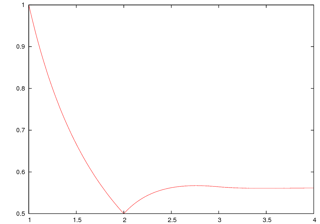
then mimics a decaying periodic function, i.e something that has similar properties to . The period of is slowly increasing, and is expected to limit to 1. Also, it has been shown that in every interval of length 1, has at least one, but no more than two, zeros. [6] If we let , and denote the critical points of the Buchstab function, [6] we have that are local minimums that are strictly increasing, and are local maximums that are strictly decreasing, in the sense that
| (4.7) | ||||
| (4.8) |
This allows us to obtain the trivial bound
| (4.9) |
Importantly, the Buchstab function decays very quickly to a constant, which makes approximating it easy for the purposes of computing Chen’s constant. For , has a closed form, and since it converges so quickly to , we can set to be a constant when is sufficiently large. Cheer–Goldston published a table of the critical points and zeros of , and by using the critical points
we can conclude using (4.7) that
| (4.10) |
For the purposes of numerically integrating , we only consider the region , as beyond that, we can set for and bound the error by (4.10).
4.2 A piecewise Taylor expansion
A closed form for the Buchstab function can be defined in a piecewise manner for each interval , as the difference equation can be rearranged such that the value in a particular interval depends on its predecessor.
Theorem 4.2.1.
Proof.
is defined for all , so by integrating (4.1),
and then by changing variables
Restrict such that .
Observe that is a constant. Call this constant .
Choose .
To force the Buchstab function to be continuous, we assume that the piecewise splines agree at the knots, that is,
So and hence
∎
By definition, . To obtain , apply (4.11).
All values of can, in principle, be obtained by repeating the above process, but they cannot be expressed in terms of elementary functions, as
is a non-elementary integral. The technique Cheer–Goldston [6] used expresses each as a power series about .
| (4.12) |
For the case of , both and are analytic, so we may write them in terms of their power series about . Cheer–Goldston shows that by doing this, one obtains
| (4.13) | ||||
| (4.14) |
We note that
Whence it follows that
To obtain the value of in general, we follow the method of Marsaglia et al. [35] and substitute (4.12) into (4.11) to obtain
| (4.15) |
The Taylor expansion of can be shown to converge uniformly in the interval , as
Hence by the Weierstrass M-test[15], the series for is uniformly convergent for . This allows us to compute the integral of the Taylor series of , (and thereby compute ) by swapping the order of the sum and the integral, by the Fubini-Tonelli theorem [46]. By using (4.11) we can prove by induction that the Taylor series of converges uniformly for . This allows interchange of the sums and integrals in (4.15). Thus, we obtain
By making a substitution we obtain
By subsequently equating coefficients of like terms we obtain the following recursive formula for , for all .
| (4.16) | ||||
| (4.17) |
where the base case and are given in (4.13). Now one can define the Buchstab function in a piecewise manner
| (4.18) |
4.2.1 Errors of Taylor expansion
In computing , we truncate the Taylor expansion to some degree , and then compute the coefficients of the resulting polynomials to a given accuracy [6]. Denote the approximation of as , and define the error to be . Define the worst case error as
By substuting into (4.11), Cheer–Goldston [6] shows that one obtains a new approximation for , with a new error term of
| (4.19) |
By repeating this argument and then by induction,
So the accuracy of holds for the rest of the , excluding computational errors due to machine precision arithmetic ‡‡‡Real number arithmetic on a computer is implemented using floating point numbers, which only have finite accuracy. Hence, every operation introduces rounding errors, and with enough operations, can cause issues with the final result.[6]. (If needed, Mathematica supports arbitrary precision arithmetic, so the magnitude of the computations errors could be made arbitrarily small.)
The error is easily computed, as by the Taylor remainder theorem [47], for every there exists a such that
| (4.20) |
Then by definition, the error term (for a Taylor expansion to order ) can be written as
| (4.21) |
So if is approximated with a power series up to order , then the maximum error for anywhere is .
4.2.2 Improving Cheer and Goldston’s Method
The approximation of the Buchstab function was improved, by computing the power series for each about . This way, was evaluated at most away from the centre of the Taylor expansion. In the previous case, could be evaluated up to 1 away from the centre. This provided a much lower error for the same degree Taylor expansion, improving the accuracy of all results using the Buchstab function. By a similar technique as above, by expanding about the middle of each interval we obtain
| (4.22) |
where
| (4.23) | ||||
| (4.24) | ||||
| (4.25) |
Applying the Taylor remainder theorem, we calculate the error of the Taylor expansion of , truncated to terms:
| (4.26) |
The coefficient can be bounded above, as
So,
| (4.27) |
Hence the error bound is improved:
| (4.28) |
which is better than the old error bound (4.21) by an exponential factor. Again, by a similar argument to (4.19), this error can be shown to hold everywhere. In practice this is a rather weak error bound, as the actual error is much less. By computing
for , (rejecting the first few until the points settle out) and plotting the values on a log plot, we observe the values form a line. By fitting a curve of the form
to this line, the asymptotic behaviour of the numerical upper bound error is deduced to be approximately . The base case for the above derivations was done with instead of as the Taylor expansion of converges slowly. The corresponding error bounds obtained are much weaker. One could, in principle, use as the base case and thus obtain a much stronger error bound for , but as mentioned above, is not an elementary function. So, is the best we could hope to use. If one used the power series expression of to compute the error bounds, each would be defined in terms of as shown,
and so, expanded out in full, the formulas for the coefficients would become (even more) unwieldy. Since the error decreases exponentially quickly with respect to the degree of the polynomial, our implementation of the Buchstab function (given above) was deemed sufficient.
Chapter 5 Numerical computations
We proceeded by implementing the above in Mathematica, using the definition of the Buchstab function given in Chapter 4. The approximation to the Buchstab function used is defined as
where is the Taylor polynomial approximation to around , to some degree (4.22). The Buchstab function was approximated using a polynomial spline over intervals, and declared equal to the limit (4.2) beyond the interval.
5.1 Justifying Integration Method
We attempted to compute the first of Wu’s integrals (3.18) without maximising with respect to
| (5.1) |
but ran into several problems. Using Mathematica’s inbuilt integration routine, the computation would either finish quickly, or never halt, depending on the value of chosen. It was discovered that the function could only be integrated for large , such that would always be in the constant region. These problems were not resolved. Instead, we integrated the Buchstab function by computing an anti-derivative of , and applying the fundamental theorem of calculus (FTC), three times.
We can show that FTC validly applies in this instance. As is a piecewise spline of polynomials, it is continuous everywhere except at the points where the splines meet. Using two theorems about Lebesgue integration [46]
Theorem 5.1.1.
If is integrable, and , then is integrable.
Theorem 5.1.2.
If is integrable on , then there exists an absolutely continuous function such that almost everywhere, and in fact we may take .
The Buchstab function is strictly positive and bounded, as (4.9). The Taylor approximation will also be non-negative and bounded, as we can easily bound the difference between and to be less than any (4.28). Thus if is defined using many splines, we can bound above by a constant on the interval . Beyond , is constant, so is integrable on any interval of the form for some . We can thus obtain FTC as
We remove the maximisation over , and set to be a function dependant on . We can convert the domain of integration
into three definite integrals, which is more suitable to apply FTC.
| (5.2) |
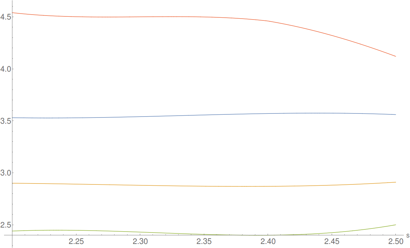
it was expected that the FTC could be used 3 times to compute , however the values computed were nonsense. When attempting to replicate the entry in Wu’s table (5.1) for , we expected and obtained a large negative result, or so. It is believed that since was defined in a piecewise manner, integrating would involve resolving many inequalities, which would only increase in complexity after three integrations.
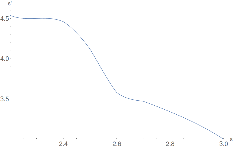
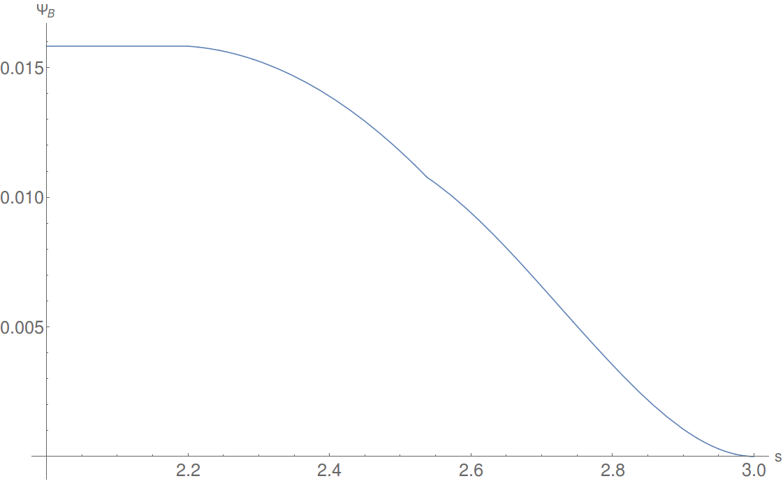
Attempts to numerically integrate were successful, however it was much faster to use Mathematica to numerically solve the differential delay equation defining the Buchstab function (4.1) with standard numerical ODE solver routines, obtain a numerical solution for , and numerically integrate the result. The resulting values were also closer to Wu’s. The following table includes Wu’s results, compared to the results we obtained.
| (Wu) | (Wu) | ||||||||
|---|---|---|---|---|---|---|---|---|---|
| 1 | 2.2 | 4.54 | 3.53 | 2.90 | 2.44 | 0.01582635 | 0.01615180 | ||
| 2 | 2.3 | 4.50 | 3.54 | 2.88 | 2.43 | 0.01224797 | 0.01547663 | ||
| 3 | 2.4 | 4.46 | 3.57 | 2.87 | 2.40 | 0.01389875 | 0.01406834 | ||
| 4 | 2.5 | 4.12 | 3.56 | 2.91 | 2.50 | 0.01177605 | 0.01187935 | ||
| 5 | 2.6 | 3.58 | 0.00940521 | 0.00947409 | |||||
| 6 | 2.7 | 3.47 | 0.00655895 | 0.00659089 | |||||
| 7 | 2.8 | 3.34 | 0.00353675 | 0.00354796 | |||||
| 8 | 2.9 | 3.19 | 0.00105665 | 0.00105838 | |||||
| 9 | 3.0 | 3.00 | 0.00000000 | 0.00000000 |
Given an , Wu chose the parameters to maximise or . All the values we calculated were an overshoot of Wu’s results, so it was not surprising that we obtained a smaller value for Chen’s constant (3.32). For , the values of Wu gave were verified to maximise our version of , by trying all values , which is given by the constraint on (3.17). So even though our did not match Wu’s, both were maximised at the same points. This indicated that we could use our “poor mans” to investigate the behaviour of , but not to compute exact values for it.
When computing the values for this table, we first wanted to see for a fixed and , how varied as a function of . It was determined that the function did not grow too quickly near the maximum, and as grew large, tended to a constant, which is consistent with quickly tending to . Thus, we can apply simple numerical maximisation techniques, without getting trapped in local maxima, or missing the maximum because the function changes too quickly. We only need to maximise over a small interval , and we obtain the maximal value by computing for a few points in the interval of interest, choosing the maximum point, and then computing again for a collection of points in a small neighbourhood about the previous maximum. This is iterated a few times until the required accuracy is obtained. (Listing 1).
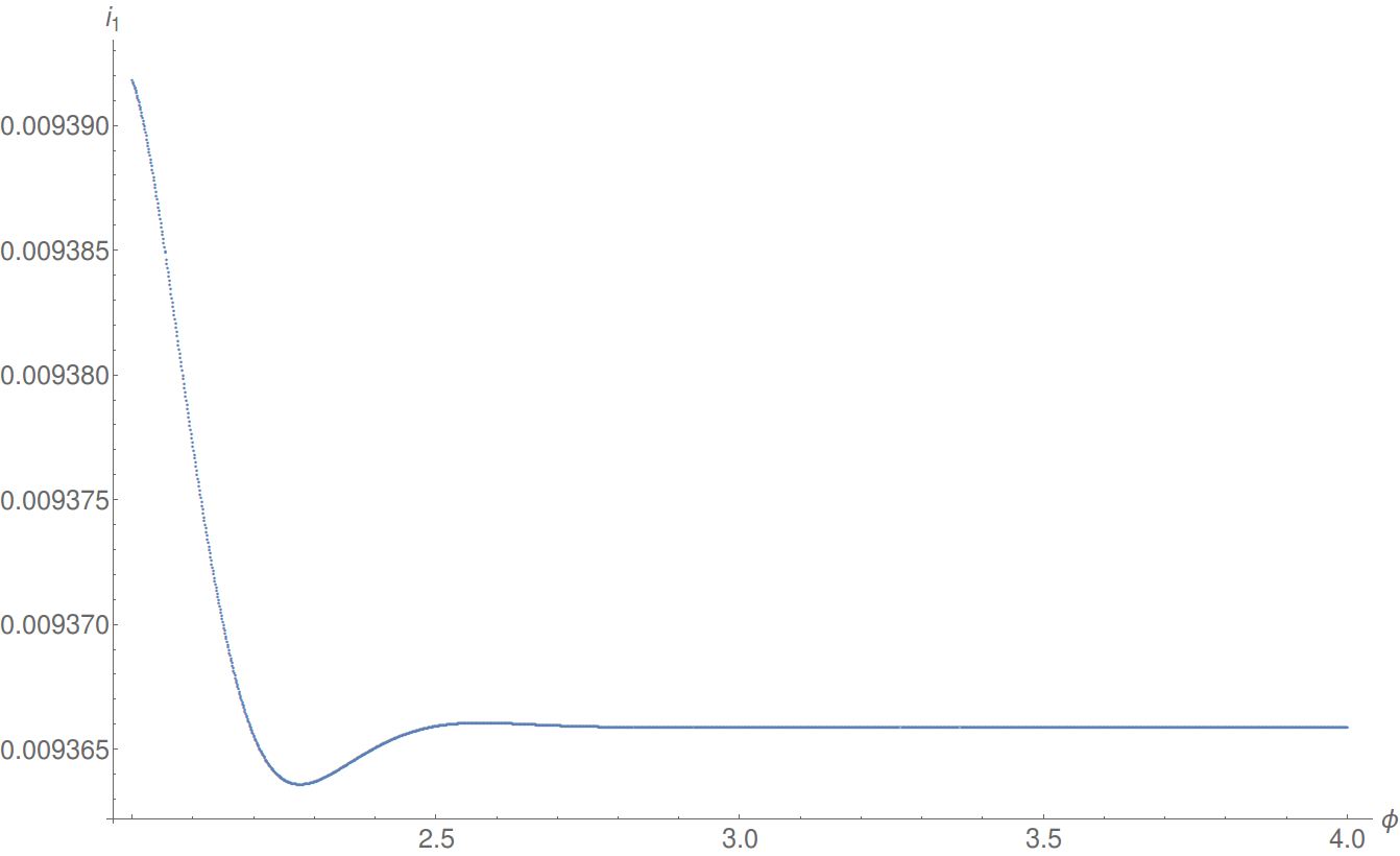
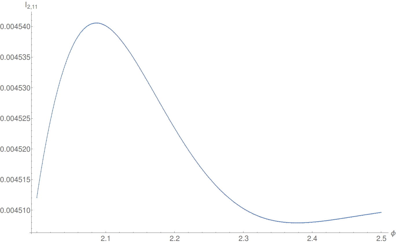
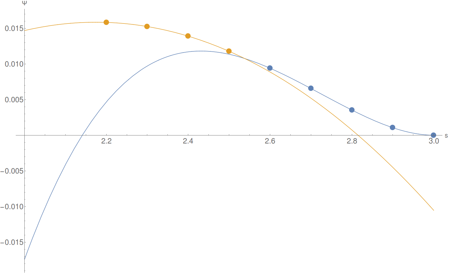
Initially, it seemed odd that for all the values of and that were tried, appeared to always be maximal when . The actual maximum for occurs at a point , but was being cut off by the constraint that . It seemed unusual to us that Wu would maximise an integral over , when the integral is always maximal when . However, for some of the other integrals in (3.21), the function was maximal at some point . This behaviour is made clear when we plot (Figure 5.2) as a function of , for a fixed value of and .
For some of the integrals needed to compute , the numerical integration did not converge. Whether this was a property of the integrals (i.e. they were not defined for those particular values of ) or a symptom of how the numerical integration routines in Mathematica operate was not determined. To maximise the integrals with respect to , we could no longer assume they were defined for all . Instead, it was found that for each integral, there would be a corresponding value such that the method of numerical integration converged for all . This value of was computed by method of bisection (Listing 2).
and can now be computed, and thus (3.17) and (3.20) can be easily computed using standard numerical integration techniques. This gives the entries of the vector (3.31). Computing the matrix (3.31) is comparatively easy, as each element of the matrix is the integral of either (see 3.16) or (see 3.16) over an interval, which is easily computed numerically. Thus, the system of linear equations (where is the identity matrix) can be solved for . This is compared to the value for that Wu obtained.
| (5.3) |
So from these vectors, we use (3.34) to obtain two different values for , ours and Wu’s,
| (5.4) |
which seems to be an improvement on Chen’s constant, but since the calculations used to obtain this value are numerical in nature and don’t match Wu’s results, it can be hard to conclude anything useful from them. Nonetheless, the effect on Chen’s constant of sampling with finer granularity was investigated. We could no longer use the table Wu had given (5.1), so we had to numerically optimise over both and . Each evaluation of is very expensive, as we have to compute each of the integrals given in (3.21). This means it is computationally difficult to compute without the corresponding parameters , as for an interval size of points, we now need to compute points, which can quickly become infeasible. We focused on increasing the sample size for , by diving the interval of into , and increasing the resolution of sampling in the interval . By defining
we use the same values before (See 5.1) for and then compute new values of for each new value of , so we evaluate at 40 points instead of 5. We can then compute by numerically maximising over , in a similar fashion to computing (See Listing 1). Note that depends on , so we are optimising with respect to two variables, and . We also need to recompute the matrix given by (3.31) on the new set of intervals. Thus, the component of is now given by
| (5.5) |
So we now have a new matrix and vector with which to solve .
Once that was complete, we redid the calculations again with even finer granularity for , choosing
These calculations were run in parallel on a computer equipped with an i5-3570K CPU overclocked to 3.80Ghz, and with 6GB of RAM.
| Points | Time | Time | ||
|---|---|---|---|---|
| Wu | - | - | 0.0223938 | 7.82085 |
| 5 | 1m27s | s | 0.0227655 | 7.8178752 |
| 40 | 11m31s | 10s | 0.0228800 | 7.81696 |
| 400 | 1h53m | 11m12s | 0.0229275 | 7.81658 |
The time taken to compute additional intervals increases rapidly, the projected time for 4000 intervals would take longer than a day to compute, with likely minimal improvement on the constant.
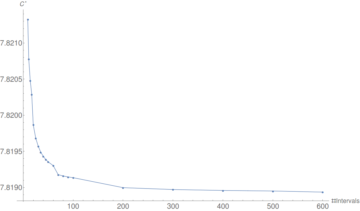
5.2 Interpolating Wu’s data
Since is complicated to evaluate, we looked at approximating it by interpolation, so see what effects additional values of would have on Chen’s constant. We assume the best possible case where possible, to obtain the best possible value for . By demonstrating that even under the best assumptions the improvements on are minimal, this should indicate that improving using Wu’s integrals will give a similarly small improvement. appears to be decreasing by Chen’s table, and so too for , so we interpolate the points with Mathematica in-built interpolation routine. By plotting the interpolant of and , we can see one overtakes the other at around . This is why Wu had split up his table in this way, choosing for the lower half and for the upper, to get the best possible bound.
We define
| (5.6) |
where is the point where . Thus, is the best case scenario, by essentially taking the maximum of the two upper bounds. We need the values for to compute , as we need to compute the matrix , which in turn depends on the values of (see 5.5). So we obtain those variables by interpolation also.
We then discretise the interval from coarse to fine, and calculate the new value of for each of these discretisations. In doing so, we can get an estimate as to how much additional intervals of integration impact the value of . After computing for a varying number of intervals, from Wu’s original 9 up to 600 (which took 84 minutes, 40 seconds on the same hardware used to compute Table 5.2), we can clearly see that adding more intervals does make a slight difference, but there are diminishing returns beyond a hundred or so. One would expect not to make any gains on by attempting to compute a million intervals.
Chapter 6 Summary
6.1 Buchstab function
We have improved on the approximation of the Buchstab function that Cheer–Goldston [6] gave. We used a spline, where each polynomial in the spline is the Taylor expansion of about the centre of the interval , whereas Cheer–Golston expanded about the right endpoint of this interval. We derived an implicit formula for the coefficients for the power series
where each is defined in terms of the previous values for , and the values of are derived from the Taylor expansion of
The coefficients are more complicated than the ones Cheer–Goldston obtained, but when the Taylor approximation of is truncated to degree , we show that the corresponding error is less than (4.28) versus Cheer–Goldston’s error bound of .
Although the spline is not continuous at the knots, the size of the discontinuities can be made arbitrarily small by increasing the degree of the power series.
6.2 Chen’s constant
An attempt was made to use our approximation to the Buchstab function to evaluate the integrals Wu gave, to place an upper bound on . This was not successful, so instead we numerically solved the ODE that defined , and numerically evaluated Wu’s integrals instead. This gave us approximately the same results as Wu. Wu resolved a set of functional inequalities using a discretisation of into 9 pieces, so we replicated the results, and then increased the resolution for the section of the interval from 5 points to 40, and then 400. The corresponding change in was as expected, minimal. The relative difference in between sampling 5 points and 400 points in the interval was only . This leads us to believe that we should expect similar results, had we computed an exact form of Wu’s integrals.
We interpolated the values of and the variables required from Wu’s data, and (under the assumption that these interpolations are a reasonable approximation to the exact form), we have shown that Wu was indeed right in asserting that cutting into more subintervals would result in a better value for , but only by a minuscule amount.
Wu gives us that is decreasing on . The constraint on the parameter is that , but Wu’s discretisation starts at . Wu claims this was chosen as attains its maximum at approximately . How close this value of is to the true maximal value is not stated, so this could be another avenue for improvement. One could explore the value of in a small neighbourhood around , to see what the true maximum is.
Slightly nudging this value left of to, say, might mean a better upper bound for , and thus a better value for Chen’s constant.
6.3 Future work
There is still a lot of work that could be done to decrease Chen’s constant. The obvious improvement is to find a way to compute ***Whenever is mentioned in this section, take it to mean both and . using the approximation of given above. We could also look at attempting to get the current implementation of running quicker, which would allow sampling more points in the interval , and finding the coefficients that make maximal, as the current version of is too slow to optimise over 5 variables simultaneously. We could look at more clever ways to maximise using more advanced numerical maximisation methods. The behaviour of is not pathological, in the sense that the functions appear to have some degree of smoothness, and the derivative is not too large. It seems true that are locally concave †††A function is concave if for any two points , the unique line that intersects and satisfies for all . near the local maximum, so once values for the variables have been found that bring near the maximum, one could then run a battery of standard convex optimisation techniques on the problem.
We could also look at alternative forms of approximating . Since we are never concerned with the values of at single points, but rather the integral of over intervals, we could look to approximations of on each interval that minimise the error
as Taylor expansions are by no means the best polynomial approximation with respect to error. Chebyshev ‡‡‡The Chebyshev polynomials are a set of polynomials defined by the recursive formula . They have the property that the error incurred by using them to approximate a function is more uniformly distributed over the interval the function is being approximated. Taylor series are exact at a single point, and the error tends to grow quickly as points move away from the center of the expansion [5]. or Hermite §§§Hermite polynomials are similar to Chebyshev polynomials, but Hermite polynomial approximation also takes into account the derivative of the function being approximated, and attempts to match both the values of the function, and it’s derivative [5]. polynomials are ideal for this purpose, and the speed of computing the approximation is not a concern, as we only need to compute the polynomial approximation of once. So the new Chebyshev approximation would be identical to the current approximation, but the polynomials would have different coefficients. We could also look at Bernstein polynomials. ¶¶¶The Bernstein polynomials are a family of polynomials, given by . This is the Bernstein polynomial for the function . It can be shown that i.e. that converges to uniformly.[15]
As is continuous, we have by the Weierstrass Approximation Theorem[15] that for any and any interval there exists a polynomial such that . Bernstein polynomials provide a constructive way to find such a polynomial . This might prove beneficial as integrating in (3.18) would prove easier if were represented as a single polynomial instead of a spline, but since is not smooth and in fact has a cusp at , the degree of a polynomial required to closely match to within say everywhere could be massive.
None of these piecewise polynomial implementations of would fix the problem of integrating (3.18), but if that problem were solved, it might permit Wu’s values to be more accurately replicated.
For more rigorous ways of showing the difficulty of improving , we could compute some additional points for Wu’s table (5.1), and then interpolate the result. The interpolation method did remarkably well at demonstrating the negligible improvements to by a finer discretisation. However, with so few points to interpolate, it is difficult to argue that our interpolant functions for are actually representative of the behaviour of . Ideally, we would want to, either by analytic or numeric methods, create an upper bound for that is in a sense “too good”, and then use that to compute . If the resulting value for was only a very small change from Wu’s value, then that provides very strong evidence that sizeable improvements on cannot be made by using Wu’s method.
Appendix A
All the code used for the results in this thesis was written in Mathematica. Important sections of the code are here, with a brief description of what they relate to. The full code used in the thesis is available upon request.
A.1 Code
Implementation of
d[n_] := If[Mod[n/2, 2] == 0, deven[n], dodd[n]]
deven[n_] := Module[{t = 0, p = 2},
     While[p <= n/2, If[PrimeQ[n - p], t++]; p = NextPrime[p]]; t]
dodd[n_] := Module[{t = 0, p = 2},
     While[p <= n/2 - 1, If[PrimeQ[n - p], t++]; p = NextPrime[p]];
  If[PrimeQ[n/2], t++]; t]
Taylor expansion of the Buchstab function .
w2*Exact[u_] := (Log[u - 1] + 1)/u;
degreeT = 10;
precisionT = MachinePrecision;
intervalsT = 5;
wT[1, u_] :=
  Evaluate[N[Normal[Series[1/u, {u, 1 + 1/2, degreeT}]], precisionT]];
wT[2, u_] :=
  Evaluate[N[
    Normal[Series[w2Exact[u], {u, 2 + 1/2, degreeT}]],
    precisionT]];
aw2 =
  N[Evaluate[
    CoefficientList[wT[2, u] /. u -> x + 2 + 1/2, x]],
   precisionT];
Clear[aw];
aw[k_, 2] := aw2[[k + 1]]
aw[0, j_] :=
 aw[0, j] = (1/(j + 1/2))*
   Sum[(aw[k, j - 1]/2^k)*(j + (-1)^k/(2*(k + 1))),
         {k, 0, degreeT}]
aw[k_, j_] :=
 aw[k, j] = (1/(j + 1/2))*(aw[k - 1, j - 1]/k - aw[k - 1, j])
wT[j_, u_] :=
 ReleaseHold[
  Hold[Sum[aw[k, j]*(u - (j + 1/2))^k, {k, 0, degreeT}]]]
wLim = Exp[-EulerGamma];
wA[u_] := Boole[u > intervalsT + 1]*wLim +
     Sum[Boole[Inequality[k, LessEqual, u, Less, k + 1]]*wT[k,
     u], {k, 1, intervalsT}]
Numerical solution to .
wN[u_] := Evaluate[w[u] /.
NDSolve[{D[u*w[u], u] == w[u - 1], w[u /; u <= 2] == 1/u}, w,
      {u, 1, 30}, WorkingPrecision -> 50]];
Defining unsafeIntegral to blindly apply FTC without checking for validity.
unsafeIntegrate[f_] := f;
unsafeIntegrate[f_, var__,
  rest___] :=
 (unsafeIntegrate[(Integrate[f, var[[1]]] /.
      var[[1]] -> var[[3]]), rest]
   - unsafeIntegrate[(Integrate[f, var[[1]]] /. var[[1]] -> var[[2]]),
     rest])
Numerically evaluating (3.18)
i1phiN[p_, sp_, s_] :=
  Quiet[ReleaseHold[NIntegrate[Boole[t <= u <= v]
  Ψ*wN[(p - t - u - v)/u]*(1/(t*u^2*v)),
      {u, sp, s}, {t, sp, s}, {v, sp, s}, MaxRecursion -> 10,
      WorkingPrecision -> MachinePrecision, MaxPoints -> 100000,
      ΨAccuracyGoal -> 20]]][[1]]
Numerically evaluating (3.21)
i2[i_, p_, s_, sp_, k1_, k2_, k3_] :=
  Piecewise[{{NIntegrate[Boole[t <= u <= v]
  Ψ*wN[(p - t - u - v)/u]*(1/(t*u^2*v)),
       {t, 1/k1, 1/k3}, {u, 1/k1, 1/k3}, {v, 1/k1, 1/k3},
       MaxRecursion -> 10,
       WorkingPrecision -> MachinePrecision, MaxPoints -> 100000,
       AccuracyGoal -> 20][[1]],
     i == 9},
     {NIntegrate[Boole[t <= u]*wN[(p - t - u - v)/u]*(1/(t*u^2*v)),
       {t, 1/k1, 1/k2}, {u, 1/k1, 1/k2}, {v, 1/k2, 1/s},
       MaxRecursion -> 10,
       WorkingPrecision -> MachinePrecision, MaxPoints -> 100000,
       AccuracyGoal -> 20][[1]],
     i == 10},
     {NIntegrate[Boole[u <= v]
     Ψ*wN[(p - t - u - v)/u]*(1/(t*u^2*v)),
       {t, 1/k1, 1/k2}, {u, 1/k2, 1/k3}, {v, 1/k2, 1/k3},
       MaxRecursion -> 10,
       WorkingPrecision -> MachinePrecision, MaxPoints -> 100000,
       AccuracyGoal -> 20][[1]],
     i == 11},
     {NIntegrate[Boole[t <= u]*wN[(p - t - u - v)/u]*(1/(t*u^2*v)),
       {t, 1/sp, 1/k1}, {u, 1/sp, 1/k1}, {v, 1/k3, 1/s},
       MaxRecursion -> 10,
       WorkingPrecision -> MachinePrecision, MaxPoints -> 100000,
       AccuracyGoal -> 20][[1]],
     i == 12},
     {NIntegrate[wN[(p - t - u - v)/u]*(1/(t*u^2*v)),
     {t, 1/sp, 1/k1}, {u, 1/k1, 1/k2}, {v, 1/k2, 1/s},
     MaxRecursion -> 10, WorkingPrecision ->
        MachinePrecision, MaxPoints -> 100000,
        AccuracyGoal -> 20][[1]],
        i == 13},
    {NIntegrate[Boole[u <= v]*wN[(p - t - u - v)/u]*(1/(t*u^2*v)),
    {t, 1/sp, 1/k1}, {u, 1/k2, 1/s}, {v, 1/k2, 1/s},
    MaxRecursion -> 10, WorkingPrecision ->
        MachinePrecision, MaxPoints -> 100000, AccuracyGoal -> 20][[1]],
        i == 14},
    {NIntegrate[wN[(p - t - u - v)/u]*(1/(t*u^2*v)),
    {t, 1/k1, 1/k2}, {u, 1/k2, 1/k3}, {v, 1/k3, 1/s},
    MaxRecursion -> 10, WorkingPrecision -> MachinePrecision,
       MaxPoints -> 100000, AccuracyGoal -> 20][[1]],
       i == 15},
    {NIntegrate[Boole[t <= u <= v <= w]
    *wN[(p - t - u - v - w)/v]*(1/(t*u*v^2*w)),
       {t, 1/k2, 1/k3}, {u, 1/k2, 1/k3}, {v, 1/k2, 1/k3},
       {w, 1/k2, 1/k3},
       MaxRecursion -> 10, WorkingPrecision -> MachinePrecision,
       MaxPoints -> 100000,
       AccuracyGoal -> 20][[1]],
       i == 16},
    {NIntegrate[Boole[t <= u <= v]
    *wN[(p - t - u - v - w)/v]*(1/(t*u*v^2*w)),
       {t, 1/k2, 1/k3}, {u, 1/k2, 1/k3}, {v, 1/k2, 1/k3},
       {w, 1/k3, 1/s},
       MaxRecursion -> 10, WorkingPrecision -> MachinePrecision,
       MaxPoints -> 100000,
       AccuracyGoal -> 20][[1]],
       i == 17},
    {NIntegrate[Boole[t <= u && v <= w]
    *wN[(p - t - u - v - w)/v]*(1/(t*u*v^2*w)),
       {t, 1/k2, 1/k3}, {u, 1/k2, 1/k3},
       {v, 1/k3, 1/s}, {w, 1/k3, 1/s},
       MaxRecursion -> 10, WorkingPrecision -> MachinePrecision,
       MaxPoints -> 100000,
       AccuracyGoal -> 20][[1]], i == 18},
    {NIntegrate[Boole[u <= v <= w]
    *wN[(p - t - u - v - w)/v]*(1/(t*u*v^2*w)),
       {t, 1/k1, 1/k2}, {u, 1/k3, 1/s}, {v, 1/k3, 1/s},
       {w, 1/k3, 1/s}, MaxRecursion -> 10,
       WorkingPrecision -> MachinePrecision,
       MaxPoints -> 100000, AccuracyGoal -> 20][[1]],
     i == 19},
     {NIntegrate[Boole[u <= v <= w]
     *wN[(p - t - u - v - w - x)/w]*
        (1/(t*u*v*w^2*x)), {t, 1/k2, 1/k3}, {u, 1/k3, 1/s},
        {v, 1/k3, 1/s}, {w, 1/k3, 1/s},
       {x, 1/k3, 1/s}, MaxRecursion -> 10,
       WorkingPrecision -> MachinePrecision,
       MaxPoints -> 100000,
       AccuracyGoal -> 20][[1]], i == 20},
    {NIntegrate[Boole[t <= u <= v <= w <= x <= y]
    Ψ*wN[(p - t - u - v - w - x - y)/x]*
        (1/(t*u*v*w*x^2*y)), {t, 1/k3, 1/s},
        {u, 1/k3, 1/s}, {v, 1/k3, 1/s},
       {w, 1/k3, 1/s}, {x, 1/k3, 1/s}, {y, 1/k3, 1/s},
       MaxRecursion -> 10,
       WorkingPrecision -> MachinePrecision, MaxPoints -> 100000,
       AccuracyGoal -> 20][[1]],
     i == 21}}]
Setting up Wu’s data
k1L[x_] := {3.53, 3.54, 3.57, 3.56}[[x]];
k2L[x_] := {2.9, 2.88, 2.87, 2.91}[[x]];
k3L[x_] := {2.44, 2.43, 2.4, 2.5}[[x]];
sL[i_] := Piecewise[{{1, i == 0}, {2.1 + 0.1*i, i > 0}}];
spL[i_] := {4.54, 4.5, 4.46, 4.12, 3.58, 3.47, 3.34, 3.19, 3.}[[i]];
Defining
psi2comp[i_, s_, s2_, k1_, k2_,
  k3_] := (-2/5)*Integrate[Log[t - 1]/t, {t, 2, s2 - 1}] -
     (2/5)*Integrate[Log[t - 1]/t, {t, 2, k1 - 1}] -
     (1/5)*Integrate[Log[t - 1]/t, {t, 2, k2 - 1}] +
     (1/5)*
   Integrate[Log[s2*t - 1]/(t*(1 - t)), {t, 1 - 1/s, 1 - 1/s2}] +
     (1/5)*
   Integrate[Log[k1*t - 1]/(t*(1 - t)), {t, 1 - 1/k3, 1 - 1/k1}] +
     (-2/5)*Sum[i2comp[i, k], {k, 9, 21}]
where i2comp gives the output of (Listing 1)
i2comp[i_, k_] := Map[Last, \[Phi]Mout[[i]]][[k - 8]]
Part of
i2Sum[i_, s_, sp_, k1_, k2_, k3_] :=
   (-2/5)*Sum[i2[k, \[Phi]Max[k, i], sL[i], spL[i],
   ΨΨ k1L[i], k2L[i], k3L[i]], {k, 9, 19}];
Implementation of (Listing 1), numerical maximisation of with respect to .
i1testMax[i_, tolmax_] := Module[{tol = 0.1, pMax, pL = pLB[i, k], pH = 5},
   While[tol > tolmax,
     pMax = MaximalBy[monitorParallelTable[Quiet[{p, i2[k, p, sL[i], spL[i], k1L[i],
              k2L[i], k3L[i]]}], {p, pL, pH, tol}, 1], Last][[1]][[1]];
      pL = Max[pMax - tol, 2]; pH = pMax + tol; tol = tol/10];
    {pMax, i2[k, pMax, sL[i], spL[i], k1L[i], k2L[i], k3L[i]]}]
Implementation of (Listing 2) to find the smallest such that the integral is still defined.
i1Find[i_, k_, {p_, pL_, pH_, tol_}] :=
  Piecewise[{{2, Quiet[Check[Quiet[i2[k, 2, sL[i], spL[i], k1L[i], k2L[i],
  k3L[i]]],
        "Null"]] != "Null"}, {i2Find2[i, k, {p, pL, pH, tol}], True}}]
i2Find[i_, k_, {p_, pL_, pH_, tol_}] :=
  Piecewise[{{(pH + pL)/2, pH - pL < tol &&
      Quiet[Check[Quiet[i2[k, (pL + pH)/2, sL[i], spL[i], k1L[i], k2L[i], k3L[i]]],
         "Null"]] != "Null"}, {i2Find2[i, k, {p, pL, (pH + pL)/2, tol}],
     Quiet[Check[Quiet[i2[k, (pL + pH)/2, sL[i], spL[i], k1L[i], k2L[i], k3L[i]]],
        "Null"]] != "Null"}, {i2Find2[i, k, {p, (pH + pL)/2, pH, tol}],
     Quiet[Check[i2[k, (pH + pL)/2, sL[i], spL[i], k1L[i], k2L[i], k3L[i]],
     "Null"]] ==
      "Null"}}]
i2Find[i_, k_, {p_, pL_, pH_, tol_}] :=
  Piecewise[{{2, Quiet[Check[Quiet[i2[k, 2, sL[i], spL[i], k1L[i], k2L[i],
  k3L[i]]],
        "Null"]] != "Null"}, {i2Find2[i, k, {p, pL, pH, tol}], True}}]
i2Find2[i_, k_, {p_, pL_, pH_, tol_}] :=
  Piecewise[{{(pH + pL)/2, pH - pL < tol &&
      Quiet[Check[Quiet[i2[k, (pL + pH)/2, sL[i], spL[i], k1L[i], k2L[i],
      k3L[i]]],
         "Null"]] != "Null"}, {i2Find2[i, k, {p, pL, (pH + pL)/2, tol}],
     Quiet[Check[Quiet[i2[k, (pL + pH)/2, sL[i], spL[i], k1L[i], k2L[i],
     k3L[i]]],
        "Null"]] != "Null"}, {i2Find2[i, k, {p, (pH + pL)/2, pH, tol}],
     Quiet[Check[i2[k, (pH + pL)/2, sL[i], spL[i], k1L[i], k2L[i], k3L[i]],
     "Null"]] ==
      "Null"}}]
Computing (5.5).
 al[i_, s_, sp_, k1_, k2_, k3_] := Piecewise[{{k1 - 2, i == 1},
 {sp - 2, i == 2},
      {sp - sp/s - 1, i == 3}, {sp - sp/k2 - 1, i == 4},
      {sp - sp/k3 - 1, i == 5},
      {sp - (2*sp)/k2, i == 6}, {sp - sp/k1 - sp/k3, i == 7},
      {sp - sp/k1 - sp/k2, i == 8},
      {k1 - k1/k2 - 1, i == 9}}];
 sig0[t_] := sig[3, t + 2, t + 1]/(1 - [3, 5, 4]);
 sig[a_, b_, c_] :=
 ΨEvaluate[unsafeIntegrate[(1/t)*Log[c/(t - 1)], {t, a, b}]];
 Xi1[t_, s_, sp_] := (0[t]/(2*t))*Log[16/((s - 1)*(sp - 1))] +
     (Boole[sp - 2 <= t <= 3]/(2*t))*Log[(t + 1)^2/((s - 1)*(sp - 1))] +
     (Boole[sp - 2 <= t <= sp - sp/s - 1]/(2*t))*Log[(t + 1)/((s - 1)*
     (sp - 1 - t))];
 a1Int[a_, b_, s_, sp_] := NIntegrate[Xi1[t, s, sp], {t, a, b}];
 a1[i_, j_] := a1Int[sL[j - 1], sL[j], sL[i], spL[i]];
and (3.23)
Xi2[t_, s_, sp_, k1_, k2_, k3_] :=
   (0[t]/(5*t))*Log[1024/((s - 1)*(sp - 1)*(k1 - 1)*(k2 - 1)
   *(k3 - 1))] +
   (Boole[sp - 2 <= t <= 3]/(5*t))*Log[(t + 1)^5/((s - 1)*
   (sp - 1)*(k1 - 1)*(k2 - 1)*(k3 - 1))] +
   (Boole[k1 - k1/k2 - 1 <= t <= k1 - 2]/(5*t))*
     Log[(t + 1)/((k2 - 1)*(k1 - 1 - t))] +
     (Boole[sp - sp/k3 - 1 <= t <= sp - 2]/(5*t))*
     Log[(t + 1)/((k3 - 1)*(sp - 1 - t))] +
     (Boole[sp - sp/s - 1 <= t <= sp - 2]/(5*t))*
     Log[(t + 1)/((s - 1)*(sp - 1 - t))] +
     (Boole[k1 - 2 <= t <= sp - 2]/(5*t))*
     Log[(t + 1)^2/((k1 - 1)*(k2 - 1))] +
     (Boole[sp - sp/k1 - sp/k3 <= t <= sp - sp/k3 - 1]/
      (5*t*(1 - t/sp)))*Log[sp^2/((k1*sp - sp - k1*t)*(k3*sp - sp - k3*t))]
       + (Boole[sp - sp/k3 - 1 <= t <= sp - sp/k1 - sp/k2]/(5*t*(1 - t/sp)))*
     Log[(sp*(sp - 1 - t))/(k1*sp - sp - k1*t)] +
    (Boole[sp - (2*sp)/k2 <= t <= sp - sp/k1 - sp/k2]/(5*t*(1 - t/sp)))*
     Log[sp/(k2*sp - sp - k2*t)] + (Boole[sp - sp/k1 - sp/k2 <= t <= sp - 2]/
      (5*t*(1 - t/sp)))*Log[sp - 1 - t];

a2Int[a_, b_, s_, sp_, k1_, k2_, k3_]
Ψ:= NIntegrate[Xi2[t, s, sp, k1, k2, k3], {t, a, b}];

a2[i_, j_] := a2Int[sL[j - 1], sL[j], sL[i], spL[i], k1L[i], k2L[i], k3L[i]];
Solving the matrix equations (3.32)
bChen = {0.015826357,
  0.015247971,
  0.013898757,
  0.011776059,
  0.009405211,
  0.006558950,
  0.003536751,
  0.001056651,
  0};
aMat = Table[a[i, j], {i, 1, 9}, {j, 1, 9}];
MatrixForm[LinearSolve[IdentityMatrix[9] - aMat, bVec]]
Code to interpolate Wu’s data and integrate over many intervals.
psi1data = Table[{sL[i], 1[[i - 4]]}, {i, 5, 9}];
psi2data = Table[{sL[i], 2[[i]]}, {i, 1, 4}];

int1 = Interpolation[psi1data];
int2 = Interpolation[psi2data];

root = s /. FindRoot[int1[s] - int2[s], {s, 2.55}];

interpsi[s_] :=
ΨPiecewise[{{int2[2.2], 2 <= s <= 2.2}, {int2[s], 2.2 <= s <= root},
     {int1[s], root <= s <= 3}}];

spdata = Table[{sL[i], spL[i]}, {i, 1, 9}]
k1data = Table[{sL[i], k1L[i]}, {i, 1, 4}];
k2data = Table[{sL[i], k2L[i]}, {i, 1, 4}];
k3data = Table[{sL[i], k3L[i]}, {i, 1, 4}];

intk1 = Interpolation[k1data];
intk2 = Interpolation[k2data];
intk3 = Interpolation[k3data];
intSp = Interpolation[spdata]

a1Int[a_, b_, s_, sp_] := NIntegrate[Xi1[t, s, sp], {t, a, b}]

sint[i_, d_] := sint[i, d] = Piecewise[{{1, i == 0},
      {Range[22/10, 3, (3 - 22/10)/(d - 1)][[i]], i > 0}}];

a1[i_, j_, d_]
Ψ:= a1Int[sint[j - 1, d], sint[j, d], sint[i, d], intSp[sint[i, d]]];

a2Int[a_, b_, s_, sp_, k1_, k2_, k3_]
Ψ:= NIntegrate[Xi2[t, s, sp, k1, k2, k3], {t, a, b}];

a2[i_, j_, d_]
Ψ:= a2Int[sint[j - 1, d], sint[j, d], sint[i, d], intSp[sint[i, d]],
    intk1[sint[i, d]], intk2[sint[i, d]], intk3[sint[i, d]]];

a[i_, j_, d_]
Ψ:= Piecewise[{{a1[i, j, d], sint[i, d] > root},
     {a2[i, j, d], sint[i, d] < root}}];

aMat[d_] := ParallelTable[a[i, j, d], {i, 1, d}, {j, 1, d}];
bsec[i_, d_] := interpsi[sint[i, d]];
bVec[d_] := Table[interpsi[sint[i, d]], {i, 1, d}];
xVec[d_] := LinearSolve[IdentityMatrix[d] - aMat[d], bVec[d]];
chen[d_] := 8*(1 - xVec[d][[1]])

Quiet[Function[x, AbsoluteTiming[{x, chen[x]}]] /@ {200, 300, 400, 500, 600}]
Bibliography
- [1] T. Apostol. Introduction to Analytic Number Theory. Undergraduate Texts in Mathematics. Springer, New York, 1998.
- [2] J. Baker. Excel and the Goldbach comet. Spreadsheets in Education (eJSiE), 2(2):2, 2007.
- [3] E. Bombieri and H. Davenport. Small differences between prime numbers. Proceedings of the Royal Society of London A: Mathematical, Physical and Engineering Sciences, 293:1–18, 1966.
- [4] A. Buchstab. Asymptotic estimate of one general number-theoretic function (Russian). Mat. Sat., 2 (44):1239–1246, 1937.
- [5] R. Burden, J. D. Faires, and A. Reynolds. Numerical analysis (1985). Prindle, Weber & Schmidt, 1985.
- [6] A. Y. Cheer and D. A. Goldston. A differential delay equation arising from the sieve of Eratosthenes. Mathematics of computation, 55(191):129–141, 1990.
- [7] J.-R. CHEN. On the Goldbach’s problem and the sieve methods. Scientia Sinica, 21(6):701–739, 1978.
- [8] Y.-G. Chen and X.-G. Sun. On romanoff’s constant. Journal of Number Theory, 106(2):275–284, 2004.
- [9] N. G. de Bruijn. On the number of uncancelled elements in the sieve of eratosthenes. Indag. math., 12:247–256, 1950.
- [10] J. De Koninck and F. Luca. Analytic Number Theory: Exploring the Anatomy of Integers. Graduate studies in mathematics. American Mathematical Society, 2012.
- [11] J.-M. Deshouillers, G. Effinger, H. Te Riele, and D. Zinoviev. A complete Vinogradov 3-primes theorem under the Riemann hypothesis. Electronic Research Announcements of the American Mathematical Society, 3(15):99–104, 1997.
- [12] T. O. e Silva. Goldbach conjecture verification, 2017. [Online; accessed 31-January-2017].
- [13] P. Erdös. On integers of the form and some related problems. Summa Brasil. Math., 2:113–125, 1950.
- [14] H. F. Fliegel and D. S. Robertson. Goldbach’s comet: the numbers related to Goldbach’s conjecture. Journal of Recreational Mathematics, 21(1):1–7, 1989.
- [15] R. Goldberg. Methods of real analysis. Blaisdell book in the pure and applied sciences. Blaisdell Pub. Co., 1964.
- [16] S. W. Golomb. The invincible primes. The Sciences, 25(2):50–57, 1985.
- [17] R. Guy. Unsolved problems in number theory. Problem books in mathematics. Springer-Verlag, 1994.
- [18] L. Habsieger and X.-F. Roblot. On integers of the form . Acta Arithmetica, 122(1):45–50, 2006.
- [19] H. Halberstam and H. Richert. Sieve methods. L.M.S. monographs. Academic Press, 1974.
- [20] G. H. Hardy and J. E. Littlewood. Some problems of ‘partitio numerorum’; iii: On the expression of a number as a sum of primes. Acta Mathematica, 44(1):1–70, 1923.
- [21] D. Heath-Brown. Lectures on sieves. arXiv preprint math/0209360, 2002.
- [22] D. R. Heath-Brown and J.-C. Puchta. Integers represented as a sum of primes and powers of two. arXiv preprint math/0201299, 2002.
- [23] H. A. Helfgott. The ternary Goldbach conjecture is true. arXiv preprint arXiv:1312.7748, 2013.
- [24] L.-K. Hua. Estimation of an integral. Sci. Sinica, 4:393–402, 1951.
- [25] H. Iwaniec. A new form of the error term in the linear sieve. Acta Arithmetica, 37(1):307–320, 1980.
- [26] C. JING-RUN. On the representation of a larger even integer as the sum of a prime and the product of at most two primes. SCIENCE CHINA Mathematics, 16(2):157, 1973.
- [27] H. Li. The number of powers of 2 in a representation of large even integers by sums of such powers and of two primes (ii). Acta Arithmetica, 96:369–379, 2001.
- [28] H. Z. Li. The number of powers of 2 in a representation of large even integers by sums of such powers and of two primes. ACTA ARITHMETICA-WARSZAWA-, 92(3):229–237, 2000.
- [29] Y. V. Linnik. Prime numbers and powers of two. Trudy Matematicheskogo Instituta imeni VA Steklova, 38:152–169, 1951.
- [30] Y. V. Linnik. Addition of prime numbers with powers of one and the same number. Matematicheskii Sbornik, 74(1):3–60, 1953.
- [31] J. Liu, M. Liu, and T. Wang. The number of powers of 2 in a representation of large even integers ii. Science in China Series A: Mathematics, 41(12):1255–1271, 1998.
- [32] J. Liu, M.-C. Liu, and T. Wang. On the almost Goldbach problem of linnik. Journal de théorie des nombres de Bordeaux, 11(1):133–147, 1999.
- [33] Z. Liu and G. LÜ. Density of two squares of primes and powers of 2. International Journal of Number Theory, 7(05):1317–1329, 2011.
- [34] T. Z. W. M. C. Liu. On the Vinogradov bound in the three primes Goldbach conjecture. Acta Arithmetica, 105(2):133–175, 2002.
- [35] G. Marsaglia, A. Zaman, and J. C. Marsaglia. Numerical solution of some classical differential-difference equations. Mathematics of Computation, 53(187):191–201, 1989.
- [36] M. E. O’NEILL. The genuine sieve of eratosthenes. Journal of Functional Programming, 19(01):95–106, 2009.
- [37] C.-D. Pan. A new application of the yu. v. linnik large sieve method. Chinese Math. Acta, 5:642–652, 1964.
- [38] J. Pintz. A note on romanov’s constant. Acta Mathematica Hungarica, 112(1-2):1–14, 2006.
- [39] J. Pintz and A. Khalfalah. On the representation of Goldbach numbers by a bounded number of powers of two. Proceedings Elementary and Analytic Number Theory, 2004.
- [40] J. Pintz and I. Ruzsa. On linnik’s approximation to Goldbach’s problem, i. Acta Arithmetica, 109(2):169–194, 2003.
- [41] D. Platt and T. Trudgian. Linnik’s approximation to Goldbach’s conjecture, and other problems. Journal of Number Theory, 153:54–62, 2015.
- [42] F. Romani. Computations concerning primes and powers of two. Calcolo, 20(3):319–336, 1983.
- [43] N. Romanoff. Über einige sätze der additiven zahlentheorie. Mathematische Annalen, 109(1):668–678, 1934.
- [44] P. Ross. On chen’s theorem that each large even number has the form or . Journal of the London Mathematical Society, 2(4):500–506, 1975.
- [45] A. Selberg. On elementary methods in primenumber-theory and their limitations. Den 11te Skandinaviske Matematikerkongress (Trondheim, 1949), Johan Grundt Tanums Forlag, Oslo, pages 13–22, 1952.
- [46] E. M. Stein and R. Shakarchi. Real analysis: measure theory, integration, and Hilbert spaces. Princeton University Press, 2009.
- [47] J. Stewart. Calculus. Cengage Learning, 2015.
- [48] T. Trudgian and J. Wu. Personal correspondance. 2013.
- [49] J. G. van der Corput. On de polignac’s conjecture. Simon Stevin, 27:99–105, 1950.
- [50] I. M. Vinogradov. Representation of an odd number as a sum of three primes. Dokl. Akad. Nauk. SSR 15, page 291–294, 1937.
- [51] T. Wang. On linnik’s almost Goldbach theorem. Science in China Series A: Mathematics, 42(11):1155–1172, 1999.
- [52] J. W. Wrench Jr. Evaluation of artin’s constant and the twin-prime constant. Mathematics of Computation, pages 396–398, 1961.
- [53] D. H. Wu. An improvement of j. r. chen’s theorem. Shanghai Keji Daxue Xuebao, pages 94–99, 1997.
- [54] J. Wu. Chen’s double sieve, Goldbach’s conjecture and the twin prime problem. Acta Arithmetica, 114:215–273, 2004.
- [55] T. Yamada. Explicit chen’s theorem. arXiv preprint arXiv:1511.03409, 2015.