Contour-time approach to the Bose-Hubbard model in the strong coupling regime: Studying two-point spatio-temporal correlations at the Hartree-Fock-Bogoliubov level

Abstract

We develop a formalism that allows the study of correlations in space and time in both the superfluid and Mott insulating phases of the Bose-Hubbard Model. Specifically, we obtain a two particle irreducible effective action within the contour-time formalism that allows for both equilibrium and out of equilibrium phenomena. We derive equations of motion for both the superfluid order parameter and two-point correlation functions. To assess the accuracy of this formalism, we study the equilibrium solution of the equations of motion and compare our results to existing strong coupling methods as well as exact methods where possible. We discuss applications of this formalism to out of equilibrium situations.

1 Introduction

The out of equilibrium dynamics of cold atoms trapped in optical lattices has received considerable attention in recent years [1, 2, 3, 4, 5, 6]. The ability to tune experimental parameters over a wide range of values in real time makes these systems very versatile and gives the opportunity to study quantum systems out of equilibrium in a controlled fashion. Quantum quenches, in which parameters in the Hamiltonian are varied in time faster than the system can respond adiabatically, e.g. when a system is driven through a quantum critical point, are a protocol that is natural to study in this context and have been studied intensely both theoretically and experimentally.

The Bose-Hubbard model (BHM) [7] has been shown to describe interacting ultracold bosons in an optical lattice [8], allowing the opportunity for experiments to probe the out of equilibrium dynamics of the model [8, 9, 10, 11, 12, 13, 14, 15, 16, 17, 18, 19, 20, 21, 22, 23, 24, 25]. The BHM is a particularly convenient context for studying quantum quenches as it displays a quantum phase transition between the superfluid and Mott-insulator phases (or vice versa) as the ratio of intersite hopping $J$ to the on-site repulsion $U$ is varied, as observed by Greiner et al. [9]. Theoretical studies of the BHM suggest that whether equilibration occurs or not after a quantum quench depends sensitively on the initial and final values of $J/U$ and the chemical potential [26, 27, 28, 29, 30, 31, 32, 33]. In the case of quenches from superfluid (large $J/U$) to Mott insulator (small $J/U$) there have been suggestions that there may be aging behaviour and glassiness that might be experimentally observable in two time correlations or in violations of the fluctuation dissipation theorem [26, 27, 28, 31, 33, 6]. In the alternative quench from Mott insulator to superfluid, it has been suggested that Kibble-Zurek [34, 35, 36] scaling of defects should be observed [37, 38], which has recently been tested experimentally [10].

In experiments, the combination of a harmonic trap and small $J/U$ leads to a wedding cake structure of the equilibrium density, with alternating Mott insulating and superfluid regions [39, 40]. The presence of Mott insulating regions has been predicted to retard relaxation to equilibrium after a quench to small $J/U$ by impeding mass transport of bosons through these regions [41, 42] which has also been observed experimentally [43]. This gives a picture in which relaxation after a quench takes place in two steps – fast relaxation to local equilibrium followed by slower relaxation via mass transport [41, 44].

In addition to slow dynamics, several analytical and numerical studies have also shown a Lieb-Robinson-like [45] bound of a maximal velocity which leads to a light-cone like spreading of density correlations in one dimensional systems for quenches from the superfluid to Mott-insulating regime as well as quenches within the superfluid [46] or Mott-insulating phases [29, 47, 42, 48]. The latter case was recently observed experimentally by Cheneau et al. [49]. Similar predictions have been made for higher dimensional systems [50, 51, 46]. The results summarized above motivate the study of the temporal and spatial correlations of the BHM after a quantum quench in order to elucidate the dynamics observed after quenches.

A generic problem in the theoretical description of quantum quenches is that it is necessary to have a formalism that is able to describe the physics in the phases on both sides of a quantum critical point. In the case of the Bose Hubbard model, numerical approaches such as exact diagonalization and the time-dependent density matrix renormalization group (t-DMRG) [26, 47, 42, 52, 53, 49, 24] can be essentially exact in all parts of parameter space but are limited by system size and usually are practical only in one dimension. For dimensions higher than one, methods such as time-dependent Gutzwiller mean field theory [4, 54, 55, 41] and dynamical mean field theory [32] have been used which can capture the presence of a quantum phase transition, but in their simplest form do not capture spatial correlations, although there has been work on including perturbative corrections [56, 57, 50, 58, 59, 60, 61]. An analytical approach based on using two Hubbard Stratonovich transformations to capture both weak-coupling and strong-coupling physics in the same formalism was developed by Sengupta and Dupuis [62]. Within their effective theory, they performed a mean-field calculation of the superfluid order parameter and a Bogoliubov (1-loop) approximation to the two-point Green’s function to study the excitation spectrum. Their work was generalized by one of us from an equilibrium theory to out of equilibrium by using the Schwinger-Keldysh formalism to obtain a one-particle irreducible (1PI) effective action which was then used to study the superfluid order parameter after a quench [31].

Here, we extend the approach developed in Ref. [31] to obtain a two-particle irreducible (2PI) effective action using the contour-time formalism, which is a generalisation of the Schwinger-Keldysh formalism. In the 2PI approach, the evolution of the order parameter and the two-point Green’s functions are treated on the same footing [63] which allows us to describe correlations both in the broken symmetry (superfluid) phase and the Mott phase. Moreover, the method provides a systematic way to go beyond the mean-field or the 1-loop approximation. We obtain two main results. First, we develop the 2PI strong coupling formalism for the BHM. Second, we derive equations of motion within a Hartree-Fock-Bogoliubov-Popov approximation suitable for both equilibrium and out of equilibrium calculations. We obtain equilibrium solutions of these equations that allow us to obtain phase boundaries and excitation spectra that we compare to previous equilibrium results obtained in a 1-loop calculation [62] and numerically exact results where possible.

This paper is structured as follows. In Section 2, we describe the model that we study and derive the 2PI effective action for the BHM. In Section 3, we obtain the equations of motion for both the order parameter and the two-particle Green’s function by taking appropriate variations of the 2PI effective action. In Section 4, we study the equilibrium solution of the equations of motion at the HFBP level. Finally in Section 5 we discuss our results and present our conclusions.

2 Model and formalism

In this section we introduce the Bose Hubbard model and discuss the generalization of the 1PI approach developed in Ref. [31] to a 2PI effective action within the Schwinger-Keldysh formalism. The Hamiltonian for the BHM, allowing for a time dependent hopping term, is

$$\hat{H}_{\text{BHM}}\left(t\right) = \hat{H}_{J}\left(t\right)+\hat{H}_{0},$$ (1)

where

$$\hat{H}_{J}\left(t\right) = -\sum_{\left\langle\vec{r}_{1},\vec{r}_{2}\right\rangle}J_{\vec{r}_{1}\vec{r}_{2}}\left(t\right)\left(\hat{a}_{\vec{r}_{1}}^{\dagger}\hat{a}_{\vec{r}_{2}}+\hat{a}_{\vec{r}_{2}}\hat{a}_{\vec{r}_{1}}^{\dagger}\right),$$ (2)

$$\hat{H}_{0}=\hat{H}_{U}-\mu\hat{N}=\frac{U}{2}\sum_{\vec{r}}\hat{n}_{\vec{r}}\left(\hat{n}_{\vec{r}}-1\right)-\mu\sum_{\vec{r}}\hat{n}_{\vec{r}},$$ (3)

with $\hat{a}_{\vec{r}}^{\dagger}$ and $\hat{a}_{\vec{r}}$ annihilation and creation operators for bosons on lattice site $\vec{r}$ respectively, $\hat{n}_{\vec{r}}\equiv\hat{a}_{\vec{r}}^{\dagger}\hat{a}_{\vec{r}}$ the number operator, $U$ the interaction strength, and $\mu$ the chemical potential. The notation $\left\langle\vec{r}_{1},\vec{r}_{2}\right\rangle$ indicates a sum over nearest neighbours only. We allow $J_{\vec{r}_{1}\vec{r}_{2}}\left(t\right)$, the hopping amplitude between sites $\vec{r}_{1}$ and $\vec{r}_{2}$, to be time dependent.

2.1 Contour-time formalism

We use the contour-time formalism [64, 65, 66, 67, 68, 69], which treats time as a complex variable lying along a contour. For systems initially prepared in thermal states, which we consider here, one can work with a contour $C$ of the form illustrated in Fig. 1. One obtains the imaginary-time Matsubara formalism, which is restricted to equilibrium problems, by setting $t_{f}=t_{i}$. If one does not work in the Matsubara formalism, $t_{f}$ can be set to $\infty$ without loss of generality [70]. Furthermore, if one were to set instead $t_{i}\to-\infty$, then one can obtain the real-time Schwinger-Keldysh closed-time path, which is suitable for both equilibrium and out of equilibrium problems, as the imaginary part of the contour would not contribute anything to the dynamics of the system. By setting $t_{i}\to-\infty$, one is effectively discarding transient effects. Since we are interested in studying transient phenomena, we do not set $t_{i}\to-\infty$ and instead work with the general contour illustrated in Fig. 1. A number of authors have applied contour-time approaches to the BHM [71, 31, 72, 73, 74, 63, 75, 76, 77, 78, 79] – our work differs from previous approaches in that we apply a 2PI approach within the contour formalism that is appropriate for strong coupling as well as weak coupling [63, 76].

Figure 1: Contour for a system initially prepared at time $t_{i}$ in a thermal state with inverse temperature $\beta$. $t_{f}$ is the maximum real-time considered in the problem, which may be set to $t_{f}\to\infty$ without loss of generality.

2.2 Green’s functions and the 1PI generating functionals

To characterize spatio-temporal correlations in the BHM we calculate contour-ordered Green’s functions (COGFs). We generalize the work in Ref. [31] to include Green’s functions with unequal numbers of annihilation and creation operators to allow for the study of broken symmetry phases. We frequently use the compact notation $\hat{a}_{\vec{r}}^{a}$ for the bosonic fields, defined by

$$\hat{a}_{\vec{r}}^{1}\equiv\hat{a}_{\vec{r}},\quad\hat{a}_{\vec{r}}^{2}\equiv\hat{a}_{\vec{r}}^{\dagger}.$$ (4)

We define the $n$-point COGF as [69]

$$G_{\vec{r}_{1}\ldots\vec{r}_{n}}^{a_{1}\ldots a_{n}}\left(\tau_{1},\ldots,\tau_{n}\right) \equiv \left(-i\right)^{n-1}\text{Tr}\left\{\hat{\rho}_{i}T_{C}\left[\hat{a}_{\vec{r}_{1}}^{a_{1}}\left(\tau_{1}\right)\ldots\hat{a}_{\vec{r}_{n}}^{a_{n}}\left(\tau_{n}\right)\right]\right\}$$ (5)

$$\equiv \left(-i\right)^{n-1}\left\langle T_{C}\left[\hat{a}_{\vec{r}_{1}}^{a_{1}}\left(\tau_{1}\right)\ldots\hat{a}_{\vec{r}_{n}}^{a_{n}}\left(\tau_{n}\right)\right]\right\rangle_{\hat{\rho}_{i}},$$

where $\hat{\rho}_{i}$ is the state operator for a thermal state representing the initial state of our system

$$\hat{\rho}_{i} = \frac{e^{-\beta\hat{H}_{\text{BHM}}\left(t_{i}\right)}}{\text{Tr}\left\{e^{-\beta\hat{H}_{\text{BHM}}\left(t_{i}\right)}\right\}},$$ (6)

and $\hat{a}_{\vec{r}}^{a}\left(\tau\right)$ are the bosonic fields in the Heisenberg picture with respect to $\hat{H}_{\text{BHM}}\left(\tau\right)$ [Eq. (1)]

$$\hat{a}_{\vec{r}}^{a}\left(\tau\right) = U^{\dagger}\left(\tau,\tau_{i}\right)\hat{a}_{\vec{r}}^{a}U\left(\tau,\tau_{i}\right),$$ (7)

$$U\left(\tau,\tau^{\prime}\right) = T_{C}\left[e^{-i\int_{C\left(\tau,\tau^{\prime}\right)}d\tau^{\prime\prime}\hat{H}_{\text{BHM}}\left(\tau^{\prime\prime}\right)}\right].$$ (8)

Here we have introduced explicitly the complex contour time argument $\tau$, the sub-contour $C\left(\tau,\tau^{\prime}\right)$ which goes from $\tau$ to $\tau^{\prime}$ along the contour $C$, and the contour time ordering operator $T_{C}$, which orders strings of operators according to their position on the contour, with operators at earlier contour times placed to the right. Note that the presence of $T_{C}$ in Eq. (5) leads to symmetry under permutations $\left\{p_{1},\ldots,p_{n}\right\}$ of the sequence $\left\{1,\ldots,n\right\}$:

$$G_{\vec{r}_{1}\ldots\vec{r}_{n}}^{a_{1}\ldots a_{n}}\left(\tau_{1},\ldots,\tau_{n}\right) = G_{\vec{r}_{p_{1}}\ldots\vec{r}_{p_{n}}}^{a_{p_{1}}\ldots a_{p_{n}}}\left(\tau_{p_{1}},\ldots,\tau_{p_{n}}\right).$$ (9)

At times it will be useful to express the contour time $\tau$ in terms of a contour label $\alpha$ (commonly called a Keldysh index) indicating a contour time located on $C_{\alpha}$ and a positive real parameter $s$ such that

$$\tau=\left(\alpha,s\right)=\begin{cases}t_{i}+s+i0^{+},&\text{if }\alpha=+,\\ t_{i}+s+i0^{-},&\text{if }\alpha=-,\\ t_{i}-is+i0^{-},&\text{if }\alpha=\mathcal{T},\end{cases}$$ (10)

e.g. we can rewrite the bosonic fields $\hat{a}_{\vec{r}}^{a}\left(\tau\right)$ as

$$\hat{a}_{\vec{r},\alpha}^{a}\left(s\right) \equiv \hat{a}_{\vec{r}}^{a}\left(\tau\right),$$ (11)

and the COGFs in Eq. (5) as

$$G_{\vec{r}_{1}\ldots\vec{r}_{n},\alpha_{1}\ldots\alpha_{n}}^{a_{1}\ldots a_{n}}\left(s_{1},\ldots,s_{n}\right) \equiv G_{\vec{r}_{1}\ldots\vec{r}_{n}}^{a_{1}\ldots a_{n}}\left(\tau_{1},\ldots,\tau_{n}\right)$$ (12)

$$= \left(-i\right)^{n-1}\left\langle T_{C}\left[\hat{a}_{\vec{r}_{1},\alpha_{1}}^{a_{1}}\left(s_{1}\right)\ldots\hat{a}_{\vec{r}_{n},\alpha_{n}}^{a_{n}}\left(s_{n}\right)\right]\right\rangle_{\hat{\rho}_{i}}.$$

In order for the Heisenberg fields $\hat{a}_{\vec{r}}^{a}\left(\tau\right)$ to be well-defined, we need to analytically continue the BHM Hamiltonian [Eq. (1)]. For the contour considered in this paper, $\hat{H}_{\text{BHM}}\left(\tau\right)$ is analytically continued as follows

$$\hat{H}_{\text{BHM}}\left(\tau\right)=\hat{H}_{\text{BHM},\alpha}\left(s\right)\equiv\begin{cases}\hat{H}_{\text{BHM}}\left(s\right),&\text{if }\alpha=+,\\ \hat{H}_{\text{BHM}}\left(s\right),&\text{if }\alpha=-,\\ \hat{H}_{\text{BHM}}\left(t_{i}\right),&\text{if }\alpha=\mathcal{T}.\end{cases}$$ (13)

The COGFs above can be derived from a generating functional $\mathcal{Z}\left[f\right]$ defined as

$$\mathcal{Z}\left[f\right] \equiv \text{Tr}\left\{\hat{\rho}_{i}T_{C}\left[e^{i\int_{C}d\tau\sum_{\vec{r}}f_{\vec{r}}^{\overline{a}}\left(\tau\right)\hat{a}_{\vec{r}}^{a}\left(\tau\right)}\right]\right\}$$ (14)

$$= \text{Tr}\left\{\hat{\rho}_{i}T_{C}\left[e^{i\left(\int_{C_{+}}+\int_{C_{-}}+\int_{C_{\mathcal{T}}}\right)d\tau\sum_{\vec{r}}f_{\vec{r}}^{\overline{a}}\left(\tau\right)\hat{a}_{\vec{r}}^{a}\left(\tau\right)}\right]\right\}$$

$$= \text{Tr}\left\{\hat{\rho}_{i}T_{C}\left[e^{i\left(\int_{0}^{\infty}ds\sum_{\vec{r}}f_{\vec{r},+}^{\overline{a}}\left(s\right)\hat{a}_{\vec{r},+}^{a}\left(s\right)+\int_{0}^{\infty}\left(-ds\right)\sum_{\vec{r}}f_{\vec{r},-}^{\overline{a}}\left(s\right)\hat{a}_{\vec{r},-}^{a}\left(s\right)+\int_{0}^{\beta}\left(-ids\right)\sum_{\vec{r}}f_{\vec{r},\mathcal{T}}^{\overline{a}}\left(s\right)\hat{a}_{\vec{r},\mathcal{T}}^{a}\left(s\right)\right)}\right]\right\}$$

$$= \text{Tr}\left\{\hat{\rho}_{i}T_{C}\left[e^{i\int_{0}^{s_{\alpha\alpha^{\prime}}^{f}}ds\sum_{\vec{r}}\tau_{\alpha\alpha^{\prime}}^{3}f_{\vec{r},\alpha}^{\overline{a}}\left(s\right)\hat{a}_{\vec{r},\alpha^{\prime}}^{a}\left(s\right)}\right]\right\},$$

where

$$\hat{\tau}^{3} = \left(\begin{array}[]{ccc}1&0&0\\ 0&-1&0\\ 0&0&-i\end{array}\right)$$ (18)

in the $\left(+,-,\mathcal{T}\right)$ basis,

$$s_{\alpha\alpha^{\prime}}^{f} = \begin{cases}\infty,&\text{if }\alpha=\alpha^{\prime}=+\,{\rm or}\,-,\\ \beta,&\text{if }\alpha=\alpha^{\prime}=\mathcal{T},\\ 0,&\text{otherwise},\end{cases}$$ (19)

the $f$s are source currents, the overscored index in $f_{\vec{r},\alpha}^{\overline{a}}\left(s\right)$ is defined by

$$f_{\vec{r},\alpha}^{\overline{a}}\left(s\right) = \sigma_{1}^{aa^{\prime}}f_{\vec{r},\alpha}^{a^{\prime}}\left(s\right),$$ (20)

and $\sigma_{i}$ is the $i^{\text{th}}$ Pauli matrix, i.e. $\overline{1}=2$ and $\overline{2}=1$. We use the Einstein summation convention for both the Keldysh and Nambu indices, i.e. matching indices implies a summation over all possible values of those indices. It is clear from the definition above that the generating functional is normalized such that $\mathcal{Z}\left[f=0\right]=1$.

To derive the COGFs in Eq. (12) from $\mathcal{Z}\left[f\right]$, we take appropriate functional derivatives with respect to the sources and set the sources to zero afterwards

$$G_{\vec{r}_{1}\ldots\vec{r}_{n},\alpha_{1}\ldots\alpha_{n}}^{a_{1}\ldots a_{n}}\left(s_{1},\ldots,s_{n}\right) = i\left(-1\right)^{n}\left(\left[\tau^{3}\right]_{\alpha_{1}\alpha_{1}^{\prime}}^{\dagger}\ldots\left[\tau^{3}\right]_{\alpha_{n}\alpha_{n}^{\prime}}^{\dagger}\right)$$ (21)

$$\quad\times\left.\frac{1}{\mathcal{Z}\left[f=0\right]}\frac{\delta^{n}\mathcal{Z}\left[f\right]}{\delta f_{\vec{r}_{1},\alpha_{1}^{\prime}}^{\overline{a_{1}}}\left(s_{1}\right)\ldots\delta f_{\vec{r}_{n},\alpha_{n}^{\prime}}^{\overline{a_{n}}}\left(s_{n}\right)}\right|_{f=0}.$$

2.3 Path integral form of $\mathcal{Z}\left[f\right]$

We cast the generating functional $\mathcal{Z}\left[f\right]$ in the path integral form [67], which for the case of the BHM is [31]

$$\mathcal{Z}\left[f\right] = \int\left[\mathcal{D}a^{a}\right]e^{iS_{\text{BHM}}\left[a\right]+iS_{f}\left[a\right]},$$ (22)

where $S_{\text{BHM}}$ is the action for the BHM, and $\int\left[\mathcal{D}a^{a}\right]$ is the coherent-state measure. We absorb overall constants into the measure as they will cancel out in the calculation of the COGFs due to the factor of $1/\mathcal{Z}\left[f=0\right]$ in Eq. (21). Note that in the path-integral formalism $a_{\vec{r},\alpha}^{1}=a_{\vec{r},\alpha}$ and $a_{\vec{r},\alpha}^{2}=a_{\vec{r},\alpha}^{*}$. In this formalism, we can rewrite averages of the form $\left\langle T_{C}\left[\ldots\right]\right\rangle_{\hat{\rho}_{i}}$ as follows

$$\left\langle T_{C}\left[\hat{a}_{\vec{r}_{1},\alpha_{1}}^{a_{1}}\left(s_{1}\right)\ldots\hat{a}_{\vec{r}_{n},\alpha_{n}}^{a_{n}}\left(s_{n}\right)\right]\right\rangle_{\hat{\rho}_{i}} \equiv \left\langle a_{\vec{r}_{1},\alpha_{1}}^{a_{1}}\left(s_{1}\right)\ldots a_{\vec{r}_{n},\alpha_{n}}^{a_{n}}\left(s_{n}\right)\right\rangle_{S_{\text{BHM}}},$$ (23)

where contour ordering is now implicit in the path integral representation [80]. In addition to the generating functional, we make extensive use of the generator of connected COGFs (CCOGFs) defined by

$$W\left[f\right] \equiv -i\ln\mathcal{Z}\left[f\right].$$ (24)

The $n$-point CCOGF $G_{\vec{r}_{1}\ldots\vec{r}_{n},\alpha_{1}\ldots\alpha_{n}}^{a_{1}\ldots a_{n},c}\left(s_{1},\ldots,s_{n}\right)$ can be obtained from $W\left[f\right]$ by calculating

$$G_{\vec{r}_{1}\ldots\vec{r}_{n},\alpha_{1}\ldots\alpha_{n}}^{a_{1}\ldots a_{n},c}\left(s_{1},\ldots,s_{n}\right) = \left.\left(-1\right)^{n-1}\left(\left[\tau^{3}\right]_{\alpha_{1}\alpha_{1}^{\prime}}^{\dagger}\ldots\left[\tau^{3}\right]_{\alpha_{n}\alpha_{n}^{\prime}}^{\dagger}\right)\frac{\delta^{n}W\left[f\right]}{\delta f_{\vec{r}_{1},\alpha_{1}^{\prime}}^{\overline{a_{1}}}\left(s_{1}\right)\ldots\delta f_{\vec{r}_{n},\alpha_{n}^{\prime}}^{\overline{a_{n}}}\left(s_{n}\right)}\right|_{f=0}$$ (25)

$$\equiv \left(-i\right)^{n-1}\left\langle a_{\vec{r}_{1},\alpha_{1}}^{a_{1}}\left(s_{1}\right)\ldots a_{\vec{r}_{n},\alpha_{n}}^{a_{n}}\left(s_{n}\right)\right\rangle_{S_{\text{BHM}}}^{c},$$

where $\left\langle\ldots\right\rangle^{c}$ indicates that only connected diagrams are kept. Note that the CCOGFs satisfy the same symmetry property as the COGFs

$$G_{\vec{r}_{1}\ldots\vec{r}_{n},\alpha_{1}\ldots\alpha_{n}}^{a_{1}\ldots a_{n},c}\left(s_{1},\ldots,s_{n}\right) = G_{\vec{r}_{p_{1}}\ldots\vec{r}_{p_{n}},\alpha_{p_{1}}\ldots\alpha_{p_{n}}}^{a_{p_{1}}\ldots a_{p_{n}},c}\left(s_{p_{1}},\ldots,s_{p_{n}}\right).$$ (26)

2.4 Keldysh rotation

For the $n$-point CCOGF defined in Eq. (25) there are $3^{n}$ Keldysh components. However, as a consequence of causality, we can eliminate $\sum_{m=0}^{n-1}\left(\begin{smallmatrix}n\\ m\end{smallmatrix}\right)$ of these components by performing the following transformation on the bosonic fields [65]

$$\left(\begin{array}[]{c}a_{+}\left(t\right)\\ a_{-}\left(t\right)\\ a_{\mathcal{T}}\left(t\right)\end{array}\right)\longrightarrow\left(\begin{array}[]{c}\tilde{a}_{q}\left(t\right)\\ \tilde{a}_{c}\left(t\right)\\ \tilde{a}_{\mathcal{T}}\left(t\right)\end{array}\right)=\hat{L}\left(\begin{array}[]{c}a_{+}\left(t\right)\\ a_{-}\left(t\right)\\ a_{\mathcal{T}}\left(t\right)\end{array}\right),$$ (27)

with

$$\hat{L} = \frac{1}{\sqrt{2}}\left(\begin{array}[]{ccc}1&-1&0\\ 1&1&0\\ 0&0&\sqrt{2}\end{array}\right),$$ (31)

where $\tilde{a}_{q}$ and $\tilde{a}_{c}$ are the quantum and classical components of the field respectively [74, 81, 82, 83], and $\tilde{a}_{\mathcal{T}}=a_{\mathcal{T}}$. After the above basis transformation $\left(+,-,\mathcal{T}\right)\to\left(q,c,\mathcal{T}\right)$, the matrix $\tau^{3}$ becomes

$$\hat{\tau}^{1} = \left(\begin{array}[]{ccc}0&1&0\\ 1&0&0\\ 0&0&-i\end{array}\right),$$ (35)

the limits of integration become

$$s_{\alpha\alpha^{\prime}}^{f} = \begin{cases}\infty,&\text{if }\left\{\alpha,\alpha^{\prime}\right\}\in P\left(\left\{q,c\right\}\right),\\ \beta,&\text{if }\alpha=\alpha^{\prime}=\mathcal{T},\\ 0,&\text{otherwise},\end{cases}$$ (36)

and $P\left(\left\{x_{m}\right\}_{m=1}^{n}\right)$ is the set of all permutations of the sequence $\left\{x_{m}\right\}_{m=1}^{n}$.

After performing the above Keldysh transformation, any COGFs $\tilde{G}_{\vec{r}_{1}\ldots\vec{r}_{n},\alpha_{1}\ldots\alpha_{n}}^{a_{1}\ldots a_{n}}\left(s_{1},\ldots,s_{n}\right)$ with at least one quantum $\alpha$-index and no classical $\alpha$-indices will vanish. To see this, consider the following COGF

$$\tilde{G}_{\vec{r}_{1}\ldots\vec{r}_{n},\underbrace{\mathcal{T}\ldots\mathcal{T}}_{m\text{ terms}}\underbrace{q\ldots q}_{n-m\text{ terms}}}^{a_{1}\ldots a_{n}}\left(s_{1},\ldots,s_{n}\right)$$

$$\quad=\left(-i\right)^{n-1}\left\langle T_{C}\left[\hat{\tilde{a}}_{\vec{r}_{1},\mathcal{T}}^{a_{1}}\left(s_{1}\right)\ldots\hat{\tilde{a}}_{\vec{r}_{m},\mathcal{T}}^{a_{m}}\left(s_{m}\right)\hat{\tilde{a}}_{\vec{r}_{m+1},q}^{a_{m+1}}\left(s_{m+1}\right)\ldots\hat{\tilde{a}}_{\vec{r}_{n},q}^{a_{n}}\left(s_{n}\right)\right]\right\rangle_{\hat{\rho}_{i}}$$

$$\quad=\frac{\left(-i\right)^{n-1}}{2^{(n-m)/2}}\left\langle T_{C}\left[\hat{a}_{\vec{r}_{1},\mathcal{T}}^{a_{1}}\left(s_{1}\right)\ldots\hat{a}_{\vec{r}_{m},\mathcal{T}}^{a_{m}}\left(s_{m}\right)\right.\right.$$

$$\left.\left.\phantom{\quad=\frac{\left(-i\right)^{n-1}}{2^{(n-m)/2}}}\quad\left\{\hat{a}_{\vec{r}_{m+1},+}^{a_{m+1}}\left(s_{m+1}\right)-\hat{a}_{\vec{r}_{m+1},-}^{a_{m+1}}\left(s_{m+1}\right)\right\}\ldots\left\{\hat{a}_{\vec{r}_{n},+}^{a_{n}}\left(s_{n}\right)-\hat{a}_{\vec{r}_{n},-}^{a_{n}}\left(s_{n}\right)\right\}\right]\right\rangle_{\hat{\rho}_{i}}$$

$$\quad=\frac{\left(-i\right)^{n-1}}{2^{(n-m)/2}}\left\langle T_{C}\left[\hat{a}_{\vec{r}_{1},\mathcal{T}}^{a_{1}}\left(s_{1}\right)\ldots\hat{a}_{\vec{r}_{m},\mathcal{T}}^{a_{m}}\left(s_{m}\right)\right]\right.$$

$$\left.\phantom{\quad=\frac{\left(-i\right)^{n-1}}{2^{(n-m)/2}}}\quad\times T_{C}\left[\left\{\hat{a}_{\vec{r}_{m+1},+}^{a_{m+1}}\left(s_{m+1}\right)-\hat{a}_{\vec{r}_{m+1},-}^{a_{m+1}}\left(s_{m+1}\right)\right\}\ldots\left\{\hat{a}_{\vec{r}_{n},+}^{a_{n}}\left(s_{n}\right)-\hat{a}_{\vec{r}_{n},-}^{a_{n}}\left(s_{n}\right)\right\}\right]\right\rangle_{\hat{\rho}_{i}}.$$ (37)

Following the argument given in Ref. [74], multiplying out the products in the second $T_{C}\left[\ldots\right]$ yields $2^{n-m}$ path-ordered terms. The key point to note is that within any one of these path-ordered products the position of the field with the largest $s$ does not depend on its Keldysh index. This implies that for each path-ordered product there is another path-ordered product is which is identical except with opposite sign. Therefore every term cancels out. It immediately follows that the associated CCOGFs vanish as well:

$$\tilde{G}_{\vec{r}_{1}\ldots\vec{r}_{n},\underbrace{\mathcal{T}\ldots\mathcal{T}}_{m\text{ terms}}\underbrace{q\ldots q}_{n-m\text{ terms}}}^{a_{1}\ldots a_{n},c}\left(s_{1},\ldots,s_{n}\right) = 0,\quad 0\leq m<n.$$ (38)

Moreover, any permutation of the Keldysh indices in Eq. (38) will also yield a vanishing CCOGF. Since there are $\left(\begin{smallmatrix}n\\ m\end{smallmatrix}\right)$ distinct permutations for fixed $n$ and $m$, there are $\sum_{m=0}^{n-1}\left(\begin{smallmatrix}n\\ m\end{smallmatrix}\right)$ components that will vanish in total. This completes the proof. Note that if we were working with a closed-time path, where there is no imaginary appendix to the contour, we recover the special case where only $\left(\begin{smallmatrix}n\\ 0\end{smallmatrix}\right)=1$ Keldysh component vanishes, namely $\tilde{G}_{\vec{r}_{1}\ldots\vec{r}_{n},q\ldots q}^{a_{1}\ldots a_{n},c}\left(s_{1},\ldots,s_{n}\right)$ [65, 74].

After performing the Keldysh transformation, the BHM action takes the form [31] (dropping tildes)

$$S_{\text{BHM}} = \frac{1}{2}\int_{0}^{s_{\alpha_{1}\alpha_{2}}^{f}}ds\sum_{\vec{r}}\left[a_{\vec{r},\alpha_{1}}^{a_{1}}\left(s\right)\left(\left[\tau^{0}\right]_{\alpha_{1}\alpha_{3}}^{\dagger}\tau_{\alpha_{3}\alpha_{2}}^{1}\sigma_{2}^{a_{1}a_{2}}\partial_{s}\right)a_{\vec{r},\alpha_{2}}^{a_{2}}\left(s\right)\right]+S_{J}+S_{U},$$ (39)

where

$$S_{J} = \frac{1}{2}\int_{0}^{s_{\alpha_{1}\alpha_{2}}^{f}}ds\sum_{\left\langle\vec{r}_{1}\vec{r}_{2}\right\rangle}a_{\vec{r}_{1},\alpha_{1}}^{a_{1}}\left(s\right)\left(2J_{\vec{r}_{1}\vec{r}_{2}}\tau_{\alpha_{1}\alpha_{2}}^{1}\sigma_{1}^{a_{1}a_{2}}\right)a_{\vec{r}_{2},\alpha_{2}}^{a_{2}}\left(s\right),$$ (40)

$$S_{U} = \frac{1}{4!}\int_{0}^{s_{\alpha_{1}\alpha_{2}\alpha_{3}\alpha_{4}}^{f}}ds\sum_{\vec{r}}\left(-U\zeta_{\alpha_{1}\alpha_{2}\alpha_{3}\alpha_{4}}^{a_{1}a_{2}a_{3}a_{4}}\right)a_{\vec{r},\alpha_{1}}^{a_{1}}\left(s\right)a_{\vec{r},\alpha_{2}}^{a_{2}}\left(s\right)a_{\vec{r},\alpha_{3}}^{a_{3}}\left(s\right)a_{\vec{r},\alpha_{4}}^{a_{4}}\left(s\right),$$ (41)

$$\hat{\tau}^{0} = \left(\begin{array}[]{ccc}1&0&0\\ 0&1&0\\ 0&0&-i\end{array}\right),$$ (45)

$$\zeta_{\alpha_{1}\alpha_{2}\alpha_{3}\alpha_{4}}^{a_{1}a_{2}a_{3}a_{4}} = 2\tau_{\alpha_{1}\alpha_{2}\alpha_{3}\alpha_{4}}\sigma^{a_{1}a_{2}a_{3}a_{4}},$$ (46)

$$\tau_{\alpha_{1}\alpha_{2}\alpha_{3}\alpha_{4}} = \begin{cases}\frac{1}{2},&\text{if }\left\{\alpha_{m}\right\}_{m=1}^{4}\in P\left(\left\{q,c,c,c\right\}\right)\bigcup P\left(\left\{c,q,q,q\right\}\right),\\ -i,&\text{if }\left\{\alpha_{m}\right\}_{m=1}^{4}=\left\{\mathcal{T},\mathcal{T},\mathcal{T},\mathcal{T}\right\},\\ 0,&\text{otherwise},\end{cases}$$ (47)

$$\sigma^{a_{1}a_{2}a_{3}a_{4}} = \begin{cases}1,&\text{if }\left\{a_{m}\right\}_{m=1}^{4}\in P\left(\left\{1,1,2,2\right\}\right),\\ 0,&\text{otherwise},\end{cases}$$ (48)

$$s_{\alpha_{1}\alpha_{2}\alpha_{3}\alpha_{4}}^{f} = \begin{cases}\infty,&\text{if }\left\{\alpha_{m}\right\}_{m=1}^{4}\in P\left(\left\{q,c,c,c\right\}\right)\bigcup P\left(\left\{c,q,q,q\right\}\right),\\ \beta,&\text{if }\left\{\alpha_{m}\right\}_{m=1}^{4}=\left\{\mathcal{T},\mathcal{T},\mathcal{T},\mathcal{T}\right\},\\ 0,&\text{otherwise}.\end{cases}$$ (49)

In the $\left(q,c,\mathcal{T}\right)$ basis, the source term becomes

$$S_{f} = \int_{0}^{s_{\alpha_{1}\alpha_{2}}^{f}}ds\sum_{\vec{r}}\tau_{\alpha_{1}\alpha_{2}}^{1}f_{\vec{r},\alpha_{1}}^{\overline{a}}\left(s\right)a_{\vec{r},\alpha_{2}}^{a}\left(s\right),$$ (50)

and the CCOGFs are

$$G_{\vec{r}_{1}\ldots\vec{r}_{n},\alpha_{1}\ldots\alpha_{n}}^{a_{1}\ldots a_{n},c}\left(s_{1},\ldots,s_{n}\right) = \left.\left(-1\right)^{n-1}\left(\left[\tau^{1}\right]_{\alpha_{1}\alpha_{1}^{\prime}}^{\dagger}\ldots\left[\tau^{1}\right]_{\alpha_{n}\alpha_{n}^{\prime}}^{\dagger}\right)\frac{\delta^{n}W\left[f\right]}{\delta f_{\vec{r}_{1},\alpha_{1}^{\prime}}^{\overline{a_{1}}}\left(s_{1}\right)\ldots\delta f_{\vec{r}_{n},\alpha_{n}^{\prime}}^{\overline{a_{n}}}\left(s_{n}\right)}\right|_{f=0}.$$ (51)

2.5 Effective theory for the Bose-Hubbard model

In order to study quench dynamics in the BHM, we make use of an effective theory that can describe both the weak and strong coupling limits of the model in the same formalism. Such an approach was developed in imaginary time by Sengupta and Dupuis [62] by using two Hubbard-Stratonovich transformations and generalized to real-time in Ref. [31]. A similar real-time theory was also obtained based on a Ginzburg-Landau approach using the Schwinger-Keldysh technique [72, 73, 74]. A brief discussion of the derivation of the effective theory along with minor corrections to several expressions presented in Ref. [31] is given in A. The effective theory obtained in Ref. [31] for the $z$ fields (which are obtained after two Hubbard Stratonovich transformations and have the same correlations as the original $a$ fields [62]) is

$$S\left[z\right] = \frac{1}{2}\int_{0}^{s_{\alpha\alpha^{\prime}}^{f}}\left(\tau_{\alpha\alpha^{\prime}}^{1}ds\right)\sum_{\left\langle\vec{r}_{1}\vec{r}_{2}\right\rangle}z_{\vec{r}_{1},\alpha}^{\overline{a}}\left(s\right)\left[2J_{\vec{r}_{1}\vec{r}_{2}}\left(s\right)\right]z_{\vec{r}_{2},\alpha^{\prime}}^{a}\left(s\right)$$ (52)

$$+\frac{1}{2}\sum_{\vec{r}}\prod_{m=1}^{2}\left[\int_{0}^{s_{\alpha_{m}\alpha_{m}^{\prime}}^{f}}\left(\tau_{\alpha_{m}\alpha_{m}^{\prime}}^{1}ds_{m}\right)z_{\vec{r},\alpha_{m}}^{a_{m}}\left(s_{m}\right)\right]\left[\left(\mathcal{G}^{c}\right)^{-1}\right]_{\alpha_{1}^{\prime}\alpha_{2}^{\prime}}^{\overline{a_{1}}\overline{a_{2}}}\left(s_{1},s_{2}\right)$$

$$+\frac{1}{4!}\sum_{\vec{r}}\prod_{m=1}^{4}\left[\int_{0}^{s_{\alpha_{m}\alpha_{m}^{\prime}}^{f}}\left(\tau_{\alpha_{m}\alpha_{m}^{\prime}}^{1}ds_{m}\right)z_{\vec{r},\alpha_{m}}^{a_{m}}\left(s_{m}\right)\right]u_{\alpha_{1}^{\prime}\alpha_{2}^{\prime}\alpha_{3}^{\prime}\alpha_{4}^{\prime}}^{\overline{a_{1}}\overline{a_{2}}\overline{a_{3}}\overline{a_{4}}}\left(s_{1},s_{2},s_{3},s_{4}\right),$$

where $\left(\mathcal{G}^{c}\right)^{-1}$ is the inverse of the two-point CCOGF in the atomic limit (i.e. $J=0$), $u^{\left(4\right)}$ is

$$u_{\alpha_{1}\alpha_{2}\alpha_{3}\alpha_{4}}^{a_{1}a_{2}a_{3}a_{4}}\left(s_{1},s_{2},s_{3},s_{4}\right) = -\prod_{m=1}^{4}\left[\int_{0}^{s_{\alpha_{m}^{\prime}\alpha_{m}^{\prime\prime}}^{f}}\left(\tau_{\alpha_{m}^{\prime}\alpha_{m}^{\prime\prime}}^{1}ds_{m}^{\prime}\right)\left[\left(\mathcal{G}^{c}\right)^{-1}\right]_{\alpha_{m}\alpha_{m}^{\prime}}^{a_{m}a_{m}^{\prime}}\left(s_{m},s_{m}^{\prime}\right)\right]$$ (53)

$$\left.\phantom{-\prod_{m=1}^{4}}\quad\times\mathcal{G}_{\alpha_{1}^{\prime\prime}\alpha_{2}^{\prime\prime}\alpha_{3}^{\prime\prime}\alpha_{4}^{\prime\prime}}^{\overline{a_{1}^{\prime}}\overline{a_{2}^{\prime}}\overline{a_{3}^{\prime}}\overline{a_{4}^{\prime}},c}\left(s_{1}^{\prime},s_{2}^{\prime},s_{3}^{\prime},s_{4}^{\prime}\right)\right.,$$

and the inverse of an arbitrary two-point function $X$ satisfies

$$\int_{0}^{s_{\alpha_{3}\alpha_{3}^{\prime}}^{f}}ds_{3}\sum_{\vec{r}_{3}}\left[X^{-1}\right]_{\vec{r}_{1}\vec{r}_{3},\alpha_{1}\alpha_{3}}^{a_{1}a_{3}}\left(s_{1},s_{3}\right)\left(\tau_{\alpha_{3}\alpha_{3}^{\prime}}^{1}\tau_{\alpha_{2}\alpha_{2}^{\prime}}^{1}X_{\vec{r}_{3}\vec{r}_{2},\alpha_{3}^{\prime}\alpha_{2}^{\prime}}^{\overline{a_{3}}\overline{a_{2}}}\left(s_{3},s_{2}\right)\right)$$

$$\quad\equiv\delta_{\vec{r}_{1}\vec{r}_{2}}\delta_{\alpha_{1}\alpha_{2}}\delta^{a_{1}a_{2}}\delta\left(s_{1}-s_{2}\right).$$ (54)

Both $\left(\mathcal{G}^{c}\right)^{-1}$ and $u^{\left(4\right)}$ are independent of site index $\vec{r}$, hence we write them without site labels. However, throughout this paper we occasionally include the site labels when it serves to provide more clarity to the reader. One would have to include the site labels if for instance one considers the BHM with a harmonic potential as is realised experimentally.

Equation (52) is the key result from Ref. [31] that we use to develop the 2PI formalism in Section 2.6. However, before applying the 2PI formalism to this action, we need to include an additional correction term:

$$S_{\text{correction}}\left[z\right] = \frac{1}{2}\sum_{\vec{r}}\prod_{m=1}^{2}\left[\int_{0}^{s_{\alpha_{m}\alpha_{m}^{\prime}}^{f}}\left(\tau_{\alpha_{m}\alpha_{m}^{\prime}}^{1}ds_{m}\right)z_{\vec{r},\alpha_{m}}^{a_{m}}\left(s_{m}\right)\right]\tilde{u}_{\alpha_{1}^{\prime}\alpha_{2}^{\prime}}^{\overline{a_{1}}\overline{a_{2}}}\left(s_{1},s_{2}\right),$$ (55)

where $\tilde{u}^{\left(2\right)}$ contains an infinite set of diagrams, although here we truncate it keeping only the lowest order term:

$$\tilde{u}_{\alpha_{1}\alpha_{2}}^{a_{1}a_{2}}\left(s_{1},s_{2}\right) = -\frac{1}{2!}\prod_{m=3}^{4}\left[\int_{0}^{s_{\alpha_{m}^{\prime}\alpha_{m}^{\prime\prime}}^{f}}\left(\tau_{\alpha_{m}^{\prime}\alpha_{m}^{\prime\prime}}^{1}ds_{m}\right)\right]u_{\alpha_{1}\alpha_{2}\alpha_{3}\alpha_{4}}^{a_{1}a_{2}a_{3}a_{4}}\left(s_{1},s_{2},s_{3},s_{4}\right)\left\{i\mathcal{G}_{\tau_{3}\tau_{4}}^{\overline{a_{3}}\overline{a_{4}},c}\left(s_{3},s_{4}\right)\right\}.$$ (56)

This correction term ensures that our equations of motion are accurate to first order in $\mathcal{G}^{\left(4\right),c}$ (see A for further discussion). Moreover, it ensures that the equations of motion for the two-point CCOGF we derive in Section 3 are exact in the atomic ($J=0$) limit, which is essential when considering quenches beginning in the atomic limit. This action also gives the exact two-point CCOGF in the noninteracting ($U=0$) limit [62]. These features make this theory particularly appealing for the study of quench dynamics, since it gives the hope that one can accurately describe the behaviour of the system in both the superfluid and Mott-insulating regimes [6].

Using the symmetry relation in Eq. (26), we also note that $\left(G^{c}\right)^{-1}$, $\tilde{u}^{\left(2\right)}$ and $u^{\left(4\right)}$ satisfy the following symmetry relations (correcting Ref. [31])

$$\left[\left(G^{c}\right)^{-1}\right]_{\vec{r}_{1}\vec{r}_{2},\alpha_{1}\alpha_{2}}^{a_{1}a_{2}}\left(s_{1},s_{2}\right) = \left[\left(G^{c}\right)^{-1}\right]_{\vec{r}_{p_{1}}\vec{r}_{p_{2}},\alpha_{p_{1}}\alpha_{p_{2}}}^{a_{p_{1}}a_{p_{2}}}\left(s_{p_{1}},s_{p_{2}}\right),$$ (57)

$$\tilde{u}_{\alpha_{1}\alpha_{2}}^{a_{1}a_{2}}\left(s_{1},s_{2}\right) = \tilde{u}_{\alpha_{p_{1}}\alpha_{p_{2}}}^{a_{p_{1}}a_{p_{2}}}\left(s_{p_{1}},s_{p_{2}}\right),$$ (58)

$$u_{\alpha_{1}\alpha_{2}\alpha_{3}\alpha_{4}}^{a_{1}a_{2}a_{3}a_{4}}\left(s_{1},s_{2},s_{3},s_{4}\right) = u_{\alpha_{p_{1}}\alpha_{p_{2}}\alpha_{p_{3}}\alpha_{p_{4}}}^{a_{p_{1}}a_{p_{2}}a_{p_{3}}a_{p_{4}}}\left(s_{p_{1}},s_{p_{2}},s_{p_{3}},s_{p_{4}}\right).$$ (59)

Similar symmetry relations for four-point functions were noted in Refs. [6, 73, 74].

2.6 2PI Formalism and the effective action

In order to obtain the full two-point CCOGF (the “full propagator” from now on), which encodes non-local spatial and temporal correlations, we adopt a 2PI approach. Unlike 1PI approaches [31, 72, 73, 74], the 2PI formalism describes the evolution of the mean field (i.e. superfluid order parameter for the BHM) and the full propagator on equal footing [63]. Several authors [63, 75, 76] have applied the 2PI formalism to the BHM to derive equations of motion for the mean field and the full propagator for weak interactions.

Here, we develop a real-time 2PI approach based on the strong-coupling theory of Sengupta and Dupuis [62, 31] to capture behaviour of correlations across a quantum quench. We adopt a compact notation where we write an arbitrary function $X$ as

$$X_{\vec{r}_{1}\ldots\vec{r}_{n},\tau_{1}\ldots\tau_{n}}^{a_{1}\ldots a_{n}}\equiv X_{\vec{r}_{1}\ldots\vec{r}_{n}}^{a_{1}\ldots a_{n}}\left(\tau_{1}\ldots\tau_{n}\right)=X_{\vec{r}_{1}\ldots\vec{r}_{n},\alpha_{1}\ldots\alpha_{n}}^{a_{1}\ldots a_{n}}\left(s_{1}\ldots s_{n}\right).$$ (60)

We extend the Einstein summation convention to the $\tau$ subindices such that for two arbitrary functions $X$ and $Y$ we have

$$\sum_{\vec{r}}X_{\vec{r},\tau}^{a}Y_{\vec{r},\tau}^{\overline{a}} = \sum_{\vec{r}}\int_{0}^{s_{\alpha\alpha^{\prime}}^{f}}\left(\tau_{\alpha\alpha^{\prime}}^{1}ds\right)X_{\vec{r},\alpha}^{a}\left(s\right)Y_{\vec{r},\alpha^{\prime}}^{\overline{a}}\left(s\right).$$ (61)

We can rewrite Eq. (52) (with the correction term [Eq. (55)] included) in the condensed notation as

$$S\left[z\right] = \frac{1}{2!}\sum_{\vec{r}_{1}\vec{r}_{2}}\left[g_{0}^{-1}\right]_{\vec{r}_{1}\vec{r}_{2},\tau_{1}\tau_{2}}^{a_{1}a_{2}}z_{\vec{r}_{1},\tau_{1}}^{\overline{a_{1}}}z_{\vec{r}_{2},\tau_{2}}^{\overline{a_{2}}}+\frac{1}{4!}u_{\tau_{1}\tau_{2}\tau_{3}\tau_{4}}^{a_{1}a_{2}a_{3}a_{4}}\sum_{\vec{r}}z_{\vec{r},\tau_{1}}^{\overline{a_{1}}}z_{\vec{r},\tau_{2}}^{\overline{a_{2}}}z_{\vec{r},\tau_{3}}^{\overline{a_{3}}}z_{\vec{r},\tau_{4}}^{\overline{a_{4}}},$$ (62)

where we have introduced the generalized inverse bare propagator $g_{0}^{-1}$

$$\left[g_{0}^{-1}\right]_{\vec{r}_{1}\vec{r}_{2},\tau_{1}\tau_{2}}^{a_{1}a_{2}} = \left[\left(\mathcal{G}^{c}\right)^{-1}\right]_{\vec{r}_{1}\vec{r}_{2},\tau_{1}\tau_{2}}^{a_{1}a_{2}}+2J_{\vec{r}_{1}\vec{r}_{2},\tau_{1}\tau_{2}}^{a_{1}a_{2}}-\frac{1}{2!}\delta_{\vec{r}_{1}\vec{r}_{2}}u_{\tau_{1}\tau_{2}\tau_{3}\tau_{4}}^{a_{1}a_{2}a_{3}a_{4}}\left(i\mathcal{G}_{\vec{r}_{1}\vec{r}_{1},\tau_{3}\tau_{4}}^{\overline{a_{3}}\overline{a_{4}},c}\right),$$ (63)

with

$$\left[\left(\mathcal{G}^{c}\right)^{-1}\right]_{\vec{r}_{1}\vec{r}_{2},\tau_{1}\tau_{2}}^{a_{1}a_{2}} = \delta_{\vec{r}_{1}\vec{r}_{2}}\left[\left(\mathcal{G}^{c}\right)^{-1}\right]_{\alpha_{1}\alpha_{2}}^{a_{1}a_{2}}\left(s_{1},s_{2}\right),$$ (64)

$$J_{\vec{r}_{1}\vec{r}_{2},\tau_{1}\tau_{2}}^{a_{1}a_{2}} = J_{\vec{r}_{1}\vec{r}_{2}}\left(s_{1}\right)\left[\tau^{1}\right]_{\alpha_{1}\alpha_{2}}^{\dagger}\sigma_{1}^{a_{1}a_{2}}\delta\left(s_{1}-s_{2}\right).$$ (65)

In the 2PI formalism [84, 70], physical quantities are expressed in terms of the mean field $\phi$ and the full propagator $G^{c}$

$$\phi_{\vec{r}_{1},\tau_{1}}^{a_{1}} \equiv \left\langle z_{\vec{r}_{1},\tau_{1}}^{a_{1}}\right\rangle,$$ (66)

$$iG_{\vec{r}_{1}\vec{r}_{2},\tau_{1}\tau_{2}}^{a_{1}a_{2},c} = \left\langle z_{\vec{r}_{1},\tau_{1}}^{a_{1}}z_{\vec{r}_{2},\tau_{2}}^{a_{2}}\right\rangle-\left\langle z_{\vec{r}_{1},\tau_{1}}^{a_{1}}\right\rangle\left\langle z_{\vec{r}_{2},\tau_{2}}^{a_{2}}\right\rangle.$$ (67)

Note that $G^{c}$ is symmetric: $G_{\vec{r}_{1}\vec{r}_{2},\tau_{1}\tau_{2}}^{a_{1}a_{2},c}=G_{\vec{r}_{2}\vec{r}_{1},\tau_{2}\tau_{1}}^{a_{2}a_{1},c}$. The equations of motion for $\phi$ and $G^{c}$ are obtained by requiring the 2PI effective action $\Gamma\left[\phi,G^{c}\right]$ be stationary with respect to variations of $\phi$ and $G^{c}$. This is similar to the 1PI case where the equations of motion for $\phi$ are obtained by requiring the 1PI effective action $\Gamma\left[\phi\right]$ to be stationary with respect to variations of $\phi$. The full propagator from the 2PI effective action allows one to take into account broken symmetry states [84, 70], which is necessary to describe quenches in the superfluid regime.

To obtain the effective action we define the 2PI generating functional for Green’s functions $\mathcal{Z}\left[f,K\right]$

$$\mathcal{Z}\left[f,K\right]=e^{iW\left[f,K\right]}=\int\left[\mathcal{D}z^{a}\right]e^{iS\left[z\right]+i\sum_{\vec{r}_{1}}f_{\vec{r}_{1},\tau_{1}}^{a_{1}}z_{\vec{r}_{1},\tau_{1}}^{\overline{a_{1}}}+\frac{i}{2}\sum_{\vec{r}_{1}\vec{r}_{2}}K_{\vec{r}_{1}\vec{r}_{2},\tau_{1}\tau_{2}}^{a_{1}a_{2}}z_{\vec{r}_{1},\tau_{1}}^{\overline{a_{1}}}z_{\vec{r}_{2},\tau_{2}}^{\overline{a_{2}}}},$$ (68)

where in addition to the single-particle source current $f$, we have included a (symmetric) two-particle source current $K$. Note that $\phi$ and $G^{c}$ are obtained by calculating the following functional derivatives of $W\left[f,K\right]$:

$$\phi_{\vec{r}_{1},\tau_{1}}^{a_{1}}=\frac{\delta W\left[f,K\right]}{\delta f_{\vec{r}_{1},\tau_{1}}^{\overline{a_{1}}}},\qquad\frac{1}{2}\left(\phi_{\vec{r}_{1},\tau_{1}}^{a_{1}}\phi_{\vec{r}_{2},\tau_{2}}^{a_{2}}+iG_{\vec{r}_{1}\vec{r}_{2},\tau_{1}\tau_{2}}^{a_{1}a_{2},c}\right)=\frac{\delta W\left[f,K\right]}{\delta K_{\vec{r}_{1}\vec{r}_{2},\tau_{1}\tau_{2}}^{\overline{a_{1}}\overline{a_{2}}}}.$$ (69)

These equations implicitly give $f$ and $K$ as functions of $\phi$ and $G^{c}$: $f=f\left[\phi,G^{c}\right]$ and $K=K\left[\phi,G^{c}\right]$. The 2PI effective action $\Gamma\left[\phi,G^{c}\right]$ is formally defined as the double Legendre transform of $W\left[f,K\right]$

$$\Gamma\left[\phi,G\right] = W\left[f,K\right]-\sum_{\vec{r}_{1}}f_{\vec{r}_{1},\tau_{1}}^{a_{1}}\phi_{\vec{r}_{1},\tau_{1}}^{\overline{a_{1}}}-\frac{1}{2}\sum_{\vec{r}_{1}\vec{r}_{2}}K_{\vec{r}_{1}\vec{r}_{2},\tau_{1}\tau_{2}}^{a_{1}a_{2}}\left(\phi_{\vec{r}_{1},\tau_{1}}^{\overline{a_{1}}}\phi_{\vec{r}_{2},\tau_{2}}^{\overline{a_{2}}}+iG_{\vec{r}_{1}\vec{r}_{2},\tau_{1}\tau_{2}}^{\overline{a_{1}}\overline{a_{2}},c}\right),$$ (70)

where $f$ and $K$ should be understood as being expressed in terms of $\phi$ and $G^{c}$. The following identities can be derived [84, 70] from Eq. (70)

$$\frac{\delta\Gamma\left[\phi,G^{c}\right]}{\delta\phi_{\vec{r}_{1},\tau_{1}}^{\overline{a_{1}}}} = -f_{\vec{r}_{1},\tau_{1}}^{a_{1}}-\sum_{\vec{r}_{1}\vec{r}_{2}}K_{\vec{r}_{1}\vec{r}_{2},\tau_{1}\tau_{2}}^{a_{1}a_{2}}\phi_{\vec{r}_{2},\tau_{2}}^{\overline{a_{2}}},$$ (71)

$$\frac{\delta\Gamma\left[\phi,G^{c}\right]}{\delta G_{\vec{r}_{1}\vec{r}_{2},\tau_{1}\tau_{2}}^{\overline{a_{1}}\overline{a_{2}},c}} = -\frac{i}{2}K_{\vec{r}_{1}\vec{r}_{2},\tau_{1}\tau_{2}}^{a_{1}a_{2}}.$$ (72)

Defining

$$\left[D^{-1}\right]_{\vec{r}_{1}\vec{r}_{2},\tau_{1}\tau_{2}}^{a_{1}a_{2}} = \frac{\delta^{2}S\left[\phi\right]}{\delta\phi_{\vec{r}_{1},\tau_{1}}^{\overline{a_{1}}}\delta\phi_{\vec{r}_{2},\tau_{2}}^{\overline{a_{2}}}}$$ (73)

$$= \left[g_{0}^{-1}\right]_{\vec{r}_{1}\vec{r}_{2},\tau_{1}\tau_{2}}^{a_{1}a_{2}}+\frac{1}{2!}\delta_{\vec{r}_{1}\vec{r}_{2}}u_{\tau_{1}\tau_{2}\tau_{3}\tau_{4}}^{a_{1}a_{2}a_{3}a_{4}}\phi_{\vec{r}_{1},\tau_{3}}^{\overline{a_{3}}}\phi_{\vec{r}_{1},\tau_{4}}^{\overline{a_{4}}},$$

the effective action can be shown to take the form [84, 70]

$$\Gamma\left[\phi,G^{c}\right] = S\left[\phi\right]+\frac{i}{2}\text{Tr}\left\{\ln\left[\left(G^{c}\right)^{-1}\right]\right\}+\frac{i}{2}\sum_{\vec{r}_{1}\vec{r}_{2}}\left[D^{-1}\right]_{\vec{r}_{1}\vec{r}_{2},\tau_{1}\tau_{2}}^{a_{1}a_{2}}G_{\vec{r}_{2}\vec{r}_{1},\tau_{2}\tau_{1}}^{\overline{a_{2}}\overline{a_{1}},c}+\Gamma_{2}\left[\phi,G^{c}\right]+\text{const},$$ (74)

where $\Gamma_{2}\left[\phi,G^{c}\right]$ is the sum of all 2PI connected vacuum diagrams in the theory with vertices determined by the action

$$S_{\text{int}}\left[\varphi;\phi\right] = u_{\tau_{1}\tau_{2}\tau_{3}\tau_{4}}^{a_{1}a_{2}a_{3}a_{4}}\sum_{\vec{r}}\left\{\frac{1}{3!}\varphi_{\vec{r},\tau_{1}}^{\overline{a_{1}}}\varphi_{\vec{r},\tau_{2}}^{\overline{a_{2}}}\varphi_{\vec{r},\tau_{3}}^{\overline{a_{3}}}\phi_{\vec{r},\tau_{4}}^{\overline{a_{4}}}+\frac{1}{4!}\varphi_{\vec{r},\tau_{1}}^{\overline{a_{1}}}\varphi_{\vec{r},\tau_{2}}^{\overline{a_{2}}}\varphi_{\vec{r},\tau_{3}}^{\overline{a_{3}}}\varphi_{\vec{r},\tau_{4}}^{\overline{a_{4}}}\right\},$$ (75)

and the propagator lines determined by $G^{c}$, i.e.

$$\Gamma_{2}\left[\phi,G^{c}\right] = -i\ln\left\{\left(\det\left\{iG^{c}\right\}\right)^{-1/2}\int\mathcal{D}\left[\varphi\right]e^{\frac{i}{2!}\sum_{\vec{r}_{1}\vec{r}_{2}}\left[\left(G^{c}\right)^{-1}\right]_{\vec{r}_{1}\vec{r}_{2},\tau_{1}\tau_{2}}^{a_{1}a_{2}}\varphi_{\vec{r}_{1},\tau_{1}}^{\overline{a_{1}}}\varphi_{\vec{r}_{2},\tau_{2}}^{\overline{a_{2}}}}e^{iS_{\text{int}}\left[\varphi;\phi\right]}\right\}^{\text{2PI}}.$$ (76)

One can use Eq. (76) along with Wick’s theorem to generate all the diagrams in $\Gamma_{2}\left[\phi,G^{c}\right]$.

Figure 2: Diagrammatic expansion of $\Gamma_{2}$ up to second-order in the four-point vertex $u^{\left(4\right)}$ (as shown as a solid dot), showing (a) the double-bubble diagram, (b) the setting sun diagram, and (c) the basketball diagram.

Figure 3: Diagrammatic representation of $u_{\tau_{1}\tau_{2}\tau_{3}\tau_{4}}^{a_{1}a_{2}a_{3}a_{4}}$, $G_{\vec{r}_{1}\vec{r}_{2},\tau_{1}\tau_{2}}^{a_{1}a_{2},c}$, and $\phi_{\vec{r}_{1},\tau_{1}}^{a_{1}}$.

The diagrammatic expansion of $\Gamma_{2}\left[\phi,G^{c}\right]$ is shown in Fig. 2 up to second-order in the four-point vertex $u^{\left(4\right)}$. The solid dots represent the interaction vertices $u^{\left(4\right)}$, the solid lines represent $G^{c}$, and the dashed lines represent $\phi$ (as illustrated in Fig. 3). In this paper, we only consider the first diagram in Fig. 2, i.e. the double-bubble (D.B.) diagram, which was also considered (along with the remaining two diagrams) in Refs. [63, 76] where the BHM was studied at weak coupling. However, there is an important distinction between the calculations here and those in Refs. [63, 76], which is that the interaction vertices in Refs. [63, 76] are local in both space and time, whereas the interaction vertices we consider are local in space but nonlocal in time – this leads to additional features in the equations of motion. The contribution from the D.B. diagram is

$$\Gamma_{2}^{\left(\text{D.B.}\right)} = \frac{1}{8}u_{\tau_{1}\tau_{2}\tau_{3}\tau_{4}}^{a_{1}a_{2}a_{3}a_{4}}\sum_{\vec{r}}\left(iG_{\vec{r}\vec{r},\tau_{1}\tau_{2}}^{\overline{a_{1}}\overline{a_{2}},c}\right)\left(iG_{\vec{r}\vec{r},\tau_{3}\tau_{4}}^{\overline{a_{3}}\overline{a_{4}},c}\right).$$ (77)

3 Equations of motion

To calculate the equations of motion, first we use Eqs. (71) and (72) and set the sources to zero, giving

$$\frac{\delta S}{\delta\phi_{\vec{r}_{1},\tau_{1}}^{\overline{a_{1}}}}+\frac{i}{2}\left[\sum_{\vec{r}_{2}\vec{r}_{3}}\frac{\delta\left[D^{-1}\right]_{\vec{r}_{2}\vec{r}_{3},\tau_{2}\tau_{3}}^{a_{2}a_{3}}}{\delta\phi_{\vec{r}_{1},\tau_{1}}^{\overline{a_{1}}}}G_{\vec{r}_{3}\vec{r}_{2},\tau_{3}\tau_{2}}^{\overline{a_{3}}\overline{a_{2}},c}\right]+\frac{\delta\Gamma_{2}}{\delta\phi_{\vec{r}_{1},\tau_{1}}^{\overline{a_{1}}}}=0,$$ (78)

and

$$i\left[\left(G^{c}\right)^{-1}\right]_{\vec{r}_{1}\vec{r}_{2},\tau_{1}\tau_{2}}^{a_{1}a_{2}} = i\left[D^{-1}\right]_{\vec{r}_{1}\vec{r}_{2},\tau_{1}\tau_{2}}^{a_{1}a_{2}}-i\left[\Sigma^{\left(2\text{PI}\right)}\right]_{\vec{r}_{1}\vec{r}_{2},\tau_{1}\tau_{2}}^{a_{1}a_{2}},$$ (79)

where the second equation is Dyson’s equation with

$$\left[\Sigma^{\left(2\text{PI}\right)}\right]_{\vec{r}_{1}\vec{r}_{2},\tau_{1}\tau_{2}}^{a_{1}a_{2}} \equiv 2i\frac{\delta\Gamma_{2}}{\delta G_{\vec{r}_{1}\vec{r}_{2},\tau_{1}\tau_{2}}^{\overline{a_{1}}\overline{a_{2}},c}},$$ (80)

the 2PI self energy.

Given the form of the bare propagator in our strong-coupling theory, the equations of motion Eq. (78) and (79) in their above formulations are not suitable for dynamical calculations. We begin by reformulating Eq. (78). First, we explicitly calculate the first term in Eq. (78)

$$\frac{\delta S}{\delta\phi_{\vec{r}_{1},\tau_{1}}^{\overline{a_{1}}}} = \sum_{\vec{r}_{2}}\left[\left(\mathcal{G}^{c}\right)^{-1}\right]_{\vec{r}_{1}\vec{r}_{2},\tau_{1}\tau_{2}}^{a_{1}a_{2}}\phi_{\vec{r}_{2},\tau_{2}}^{\overline{a_{2}}}+\sum_{\vec{r}_{2}}2J_{\vec{r}_{1}\vec{r}_{2},\tau_{1}\tau_{2}}^{a_{1}a_{2}}\phi_{\vec{r}_{2},\tau_{2}}^{\overline{a_{2}}}$$ (81)

$$-\frac{1}{2!}u_{\tau_{1}\tau_{2}\tau_{3}\tau_{4}}^{a_{1}a_{2}a_{3}a_{4}}\phi_{\vec{r}_{1},\tau_{2}}^{\overline{a_{2}}}\left(i\mathcal{G}_{\vec{r}_{1}\vec{r}_{1},\tau_{3}\tau_{4}}^{\overline{a_{3}}\overline{a_{4}},c}\right)+\frac{1}{3!}u_{\tau_{1}\tau_{2}\tau_{3}\tau_{4}}^{a_{1}a_{2}a_{3}a_{4}}\phi_{\vec{r}_{1},\tau_{2}}^{\overline{a_{2}}}\phi_{\vec{r}_{1},\tau_{3}}^{\overline{a_{3}}}\phi_{\vec{r}_{1},\tau_{4}}^{\overline{a_{4}}}.$$

The second term in Eq. (78) can be written as

$$\frac{i}{2}\left[\sum_{\vec{r}_{2}\vec{r}_{3}}\frac{\delta\left[D^{-1}\right]_{\vec{r}_{2}\vec{r}_{3},\tau_{2}\tau_{3}}^{a_{2}a_{3}}}{\delta\phi_{\vec{r}_{1},\tau_{1}}^{\overline{a_{1}}}}G_{\vec{r}_{3}\vec{r}_{2},\tau_{3}\tau_{2}}^{\overline{a_{3}}\overline{a_{2}},c}\right] = \frac{1}{2!}u_{\tau_{1}\tau_{2}\tau_{3}\tau_{4}}^{a_{1}a_{2}a_{3}a_{4}}\phi_{\vec{r}_{1},\tau_{2}}^{\overline{a_{2}}}\left(iG_{\vec{r}_{1}\vec{r}_{1},\tau_{3}\tau_{4}}^{\overline{a_{3}}\overline{a_{4}},c}\right).$$ (82)

We act on both sides of Eq. (78) with $\mathcal{G}^{c}$ from the left and rearrange terms to get

$$\phi_{\vec{r}_{1},\tau_{1}}^{a_{1}} = \mathcal{G}_{\vec{r}_{1}\vec{r}_{2},\tau_{1}\tau_{2}}^{a_{1}a_{2},c}\Omega_{\vec{r}_{1},\tau_{2}}^{\overline{a_{2}}},$$ (83)

where we have introduced the quantity

$$\Omega_{\vec{r}_{1},\tau_{1}}^{a_{1}} = -\sum_{\vec{r}_{2}}2J_{\vec{r}_{1}\vec{r}_{2},\tau_{1}\tau_{2}}^{a_{1}a_{2}}\phi_{\vec{r}_{2},\tau_{2}}^{\overline{a_{2}}}-\frac{1}{3!}u_{\tau_{1}\tau_{2}\tau_{3}\tau_{4}}^{a_{1}a_{2}a_{3}a_{4}}\phi_{\vec{r}_{1},\tau_{2}}^{\overline{a_{2}}}\phi_{\vec{r}_{1},\tau_{3}}^{\overline{a_{3}}}\phi_{\vec{r}_{1},\tau_{4}}^{\overline{a_{4}}}$$ (84)

$$-\frac{1}{2!}u_{\tau_{1}\tau_{2}\tau_{3}\tau_{4}}^{a_{1}a_{2}a_{3}a_{4}}\phi_{\vec{r}_{1},\tau_{2}}^{\overline{a_{2}}}\left(iG_{\vec{r}_{1}\vec{r}_{1},\tau_{3}\tau_{4}}^{\overline{a_{3}}\overline{a_{4}},c}-i\mathcal{G}_{\vec{r}_{1}\vec{r}_{1},\tau_{3}\tau_{4}}^{\overline{a_{3}}\overline{a_{4}},c}\right)-\frac{\delta\Gamma_{2}}{\delta\phi_{\vec{r}_{1},\tau_{1}}^{\overline{a_{1}}}}.$$

Eq. (83) is a much more suitable form for dynamical calculations.

Next we reformulate Eq. (79) into a more appropriate form. First, we separate $\left[D^{-1}\right]_{\vec{r}_{1}\vec{r}_{2},\tau_{1}\tau_{2}}^{a_{1}a_{2}}$ as follows

$$\left[D^{-1}\right]_{\vec{r}_{1}\vec{r}_{2},\tau_{1}\tau_{2}}^{a_{1}a_{2}} = \left[\left(\mathcal{G}^{c}\right)^{-1}\right]_{\vec{r}_{1}\vec{r}_{2},\tau_{1}\tau_{2}}^{a_{1}a_{2}}-\left[\Sigma^{\left(1\right)}\right]_{\vec{r}_{1}\vec{r}_{2},\tau_{1}\tau_{2}}^{a_{1}a_{2}},$$ (85)

where

$$\left[\Sigma^{\left(1\right)}\right]_{\vec{r}_{1}\vec{r}_{2},\tau_{1}\tau_{2}}^{a_{1}a_{2}} = -2J_{\vec{r}_{1}\vec{r}_{2},\tau_{1}\tau_{2}}^{a_{1}a_{2}}+\frac{1}{2!}\delta_{\vec{r}_{1}\vec{r}_{2}}u_{\tau_{1}\tau_{2}\tau_{3}\tau_{4}}^{a_{1}a_{2}a_{3}a_{4}}\left(i\mathcal{G}_{\vec{r}_{1}\vec{r}_{1},\tau_{3}\tau_{4}}^{\overline{a_{3}}\overline{a_{4}},c}\right)-\frac{1}{2!}\delta_{\vec{r}_{1}\vec{r}_{2}}u_{\tau_{1}\tau_{2}\tau_{3}\tau_{4}}^{a_{1}a_{2}a_{3}a_{4}}\phi_{\vec{r}_{1},\tau_{3}}^{\overline{a_{3}}}\phi_{\vec{r}_{1},\tau_{4}}^{\overline{a_{4}}},$$ (86)

is the $1$-loop contribution to the total self energy. If we define the full self energy as

$$\Sigma_{\vec{r}_{1}\vec{r}_{2},\tau_{1}\tau_{2}}^{a_{1}a_{2}} \equiv \left[\Sigma^{\left(1\right)}\right]_{\vec{r}_{1}\vec{r}_{2},\tau_{1}\tau_{2}}^{a_{1}a_{2}}+\left[\Sigma^{\left(2\text{PI}\right)}\right]_{\vec{r}_{1}\vec{r}_{2},\tau_{1}\tau_{2}}^{a_{1}a_{2}},$$ (87)

then Eq. (79) becomes

$$i\left[\left(G^{c}\right)^{-1}\right]_{\vec{r}_{1}\vec{r}_{2},\tau_{1}\tau_{2}}^{a_{1}a_{2}} = i\left[\left(\mathcal{G}^{c}\right)^{-1}\right]_{\vec{r}_{1}\vec{r}_{2},\tau_{1}\tau_{2}}^{a_{1}a_{2}}-i\Sigma_{\vec{r}_{1}\vec{r}_{2},\tau_{1}\tau_{2}}^{a_{1}a_{2}}.$$ (88)

After rearranging a few terms, one obtains

$$G_{\vec{r}_{1}\vec{r}_{2}\tau_{1}\tau_{2}x_{2}}^{a_{1}a_{2},c} = \mathcal{G}_{\vec{r}_{1}\vec{r}_{2},\tau_{1}\tau_{2}}^{a_{1}a_{2},c}+\sum_{\vec{r}_{3}\vec{r}_{4}}\mathcal{G}_{\vec{r}_{1}\vec{r}_{3},\tau_{1}\tau_{3}}^{a_{1}a_{3},c}\Sigma_{\vec{r}_{3}\vec{r}_{4},\tau_{3}\tau_{4}}^{\overline{a_{3}}\overline{a_{4}}}G_{\vec{r}_{4}\vec{r}_{2},\tau_{4}\tau_{2}}^{a_{4}a_{2},c},$$ (89)

which is a more suitable form for dynamical calculations. That being said, the form shown here is still not particularly amenable to solution. We now discuss simplifications that allow us to obtain equations of motion that are easier to solve.

3.1 Low-frequency approximation

Equations (83) and (89), whilst having a compact form in our notation, contain as many as four time-integrals, making it computationally expensive to solve the equations numerically. This suggests that some level of approximation is required in order to obtain more physical insight from the equations above. Following Refs. [31], we focus on the low frequency components of the equations of motion. In a quench protocol this would correspond to considering changes that are slow enough that the equations of motion are dominated by low frequency terms. The approximation also applies to equilibrium calculations where there is no quench at all.

The low-frequency approximation we consider involves taking the static-limit of the four-point vertex $u^{\left(4\right)}$. If we only consider values of the chemical potential away from the degeneracy points between adjacent Mott lobes, i.e. $\mu\not\approx Ur$, with $r$ an integer, then the static limit of $u^{\left(4\right)}$ can be expressed as [62, 31, 74]

$$u_{\tau_{1}\tau_{2}\tau_{3}\tau_{4}}^{a_{1}a_{2}a_{3}a_{4}} \approx -u_{1}\delta\left(s_{1}-s_{2}\right)\delta\left(s_{1}-s_{3}\right)\delta\left(s_{1}-s_{4}\right)\zeta_{\alpha_{1}\alpha_{2}\alpha_{3}\alpha_{4}}^{a_{1}a_{2}a_{3}a_{4}}$$ (90)

$$+iu_{2}^{2}\left[\delta\left(s_{1}-s_{2}\right)\delta\left(s_{3}-s_{4}\right)\eta_{\alpha_{1}\alpha_{2}\alpha_{3}\alpha_{4}}^{a_{1}a_{2}a_{3}a_{4}}+\left\{2\leftrightarrow 3\right\}+\left\{2\leftrightarrow 4\right\}\right],$$

where $u_{1}$ and $u_{2}^{2}$ are defined in D, $\zeta_{\alpha_{1}\alpha_{2}\alpha_{3}\alpha_{4}}^{a_{1}a_{2}a_{3}a_{4}}$ is defined in Eq. (46) and

$$\eta_{\alpha_{1}\alpha_{2}\alpha_{3}\alpha_{4}}^{a_{1}a_{2}a_{3}a_{4}} \equiv \sigma_{1}^{a_{1}a_{2}}\sigma_{1}^{a_{3}a_{4}}\begin{cases}\tau_{\alpha_{1}\alpha_{2}}^{1}\tau_{\alpha_{3}\alpha_{4}}^{1}&\text{if }\alpha_{m}=q\text{ or }c\text{ for }m=1,\ldots 4\\ 0&\text{otherwise}\end{cases}.$$ (91)

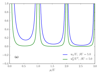
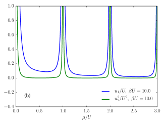
Figure 4: (Color online) (a) Plot of $u_{1}$ and $u_{2}^{2}$ as a function of $\mu/U$ for inverse temperature $\beta U=5.0$; and (b) for $\beta U=10.0$.

Numerical evaluation of $u_{1}$ and $u_{2}^{2}$ for a homogeneous system, shown in Fig. 4 demonstrates that unless $\mu/U$ is close to an integer, the $u_{1}$ terms will dominate the $u_{2}^{2}$ terms. Moreover, for low temperatures, $u_{2}^{2}$ becomes negligible and goes to zero as $\beta\to\infty$. Hence, to simplify the equations of motion, we further assume that the temperature is sufficiently low such that $u_{2}^{2}$ can be safely ignored. The end result is that the equations of motion contain single time-integrals only.

3.2 Keldysh structure of $\phi$, $G^{c}$, $\Omega$, $\Sigma$

Before presenting numerical results, it is worth discussing the explicit Keldysh structure of the mean field $\phi$, full propagator $G^{c}$, and their respective interaction terms $\Sigma$ and $\Omega$. Starting with the mean field $\phi$, we have

$$\left[\phi\right] = \left(\begin{array}[]{c}0\\ \sqrt{2}\phi_{\vec{r}_{1}}^{a_{1}}\left(s_{1}\right)\\ \phi_{\vec{r}_{1}}^{a_{1}}\left(s^{\prime}=0\right)\end{array}\right),$$ (95)

where $\phi_{\vec{r}_{1}}^{a_{1}}\left(s_{1}\right)$ is the superfluid order parameter

$$\phi_{\vec{r}_{1}}^{a_{1}}\left(s_{1}\right) = \left\langle\hat{a}_{\vec{r}_{1}}^{a_{1}}\left(t_{i}+s_{1}\right)\right\rangle_{\hat{\rho}_{i}}.$$ (96)

Note that $\phi_{\vec{r}_{1}}^{2}\left(s_{1}\right)=\left[\phi_{\vec{r}_{1}}\left(s_{1}\right)\right]^{*}$. Then, following Ref. [85], we can express $G^{c}$ as follows

$$\left[G^{c}\right] = \left(\begin{array}[]{ccc}0&G_{\vec{r}_{1}\vec{r}_{2}}^{a_{1}a_{2},\left(A\right)}\left(s_{1},s_{2}\right)&0\\ G_{\vec{r}_{1}\vec{r}_{2}}^{a_{1}a_{2},\left(R\right)}\left(s_{1},s_{2}\right)&G_{\vec{r}_{1}\vec{r}_{2}}^{a_{1}a_{2},\left(K\right)}\left(s_{1},s_{2}\right)&\sqrt{2}G_{\vec{r}_{1}\vec{r}_{2}}^{a_{1}a_{2},\left(\rceil\right)}\left(s_{1},s_{2}\right)\\ 0&\sqrt{2}G_{\vec{r}_{1}\vec{r}_{2}}^{a_{1}a_{2},\left(\lceil\right)}\left(s_{1},s_{2}\right)&iG_{\vec{r}_{1}\vec{r}_{2}}^{a_{1}a_{2},\left(M\right)}\left(s_{1},s_{2}\right)\end{array}\right),$$ (100)

with

$$G_{\vec{r}_{1}\vec{r}_{2}}^{a_{1}a_{2},\left(R\right)}\left(s_{1},s_{2}\right) \equiv -i\Theta\left(s_{1}-s_{2}\right)\left\langle\hat{a}_{\vec{r}_{1}}^{a_{1}}\left(t_{i}+s_{1}\right)\hat{a}_{\vec{r}_{2}}^{a_{2}}\left(t_{i}+s_{2}\right)-\hat{a}_{\vec{r}_{2}}^{a_{2}}\left(t_{i}+s_{2}\right)\hat{a}_{\vec{r}_{1}}^{a_{1}}\left(t_{i}+s_{1}\right)\right\rangle_{\hat{\rho}_{i}}^{c},$$ (101)

$$G_{\vec{r}_{1}\vec{r}_{2}}^{a_{1}a_{2},\left(A\right)}\left(s_{1},s_{2}\right) \equiv i\Theta\left(s_{2}-s_{1}\right)\left\langle\hat{a}_{\vec{r}_{1}}^{a_{1}}\left(t_{i}+s_{1}\right)\hat{a}_{\vec{r}_{2}}^{a_{2}}\left(t_{i}+s_{2}\right)-\hat{a}_{\vec{r}_{2}}^{a_{2}}\left(t_{i}+s_{2}\right)\hat{a}_{\vec{r}_{1}}^{a_{1}}\left(t_{i}+s_{1}\right)\right\rangle_{\hat{\rho}_{i}}^{c},$$ (102)

$$G_{\vec{r}_{1}\vec{r}_{2}}^{a_{1}a_{2},\left(K\right)}\left(s_{1},s_{2}\right) \equiv -i\left\langle\hat{a}_{\vec{r}_{1}}^{a_{1}}\left(t_{i}+s_{1}\right)\hat{a}_{\vec{r}_{2}}^{a_{2}}\left(t_{i}+s_{2}\right)+\hat{a}_{\vec{r}_{2}}^{a_{2}}\left(t_{i}+s_{2}\right)\hat{a}_{\vec{r}_{1}}^{a_{1}}\left(t_{i}+s_{1}\right)\right\rangle_{\hat{\rho}_{i}}^{c},$$ (103)

$$G_{\vec{r}_{1}\vec{r}_{2}}^{a_{1}a_{2},\left(\lceil\right)}\left(s_{1},s_{2}\right) \equiv -i\left\langle\hat{a}_{\vec{r}_{1}}^{a_{1}}\left(t_{i}-is_{1}\right)\hat{a}_{\vec{r}_{2}}^{a_{2}}\left(t_{i}+s_{2}\right)\right\rangle_{\hat{\rho}_{i}}^{c},$$ (104)

$$G_{\vec{r}_{1}\vec{r}_{2}}^{a_{1}a_{2},\left(\rceil\right)}\left(s_{1},s_{2}\right) \equiv -i\left\langle\hat{a}_{\vec{r}_{2}}^{a_{2}}\left(t_{i}-is_{2}\right)\hat{a}_{\vec{r}_{1}}^{a_{1}}\left(t_{i}+s_{1}\right)\right\rangle_{\hat{\rho}_{i}}^{c},$$ (105)

$$G_{\vec{r}_{1}\vec{r}_{2}}^{a_{1}a_{2},\left(M\right)}\left(s_{1},s_{2}\right) \equiv -\left(\Theta\left(s_{1}-s_{2}\right)\left\langle\hat{a}_{\vec{r}_{1}}^{a_{1}}\left(t_{i}-is_{1}\right)\hat{a}_{\vec{r}_{2}}^{a_{2}}\left(t_{i}-is_{2}\right)\right\rangle_{\hat{\rho}_{i}}^{c}\right.$$ (106)

$$\phantom{-}\left.\quad+\Theta\left(s_{2}-s_{1}\right)\left\langle\hat{a}_{\vec{r}_{2}}^{a_{2}}\left(t_{i}-is_{2}\right)\hat{a}_{\vec{r}_{1}}^{a_{1}}\left(t_{i}-is_{1}\right)\right\rangle_{\hat{\rho}_{i}}^{c}\right),$$

where $G^{\left(R\right)}$ and $G^{\left(A\right)}$ are the retarded and advanced Green’s functions respectively, $G^{\left(K\right)}$ is the Keldysh or Kinetic Green’s function, $G^{\left(\lceil\right)}$ and $G^{\left(\rceil\right)}$ are the left and right Green’s functions respectively, and $G^{\left(M\right)}$ is the Matsubara Green’s function.

Next we have $\Omega$, which takes on the following Keldysh structure

$$\left[\Omega\right] = \left(\begin{array}[]{c}0\\ \sqrt{2}\Omega_{\vec{r}_{1}}^{a_{1}}\left(s_{1}\right)\\ \Omega_{\vec{r}_{1}}^{a_{1}}\left(s^{\prime}=0\right)\end{array}\right),$$ (110)

where to first order in $u_{1}$ we have

$$\Omega_{\vec{r}_{1}}^{a_{1}}\left(s_{1}\right) \approx -\sum_{\vec{r}_{2}}2J_{\vec{r}_{1}\vec{r}_{2}}\left(t_{i}+s_{1}\right)\phi_{\vec{r}_{2}}^{a_{1}}\left(s_{1}\right)+u_{1}\left|\phi_{\vec{r}_{1}}\left(s_{1}\right)\right|^{2}\phi_{\vec{r}_{1}}^{a_{1}}\left(s_{1}\right)$$ (111)

$$\phantom{-\sum_{\vec{r}_{2}}}+\frac{u_{1}}{2}\sigma^{a_{1}a_{2}a_{3}a_{4}}\phi_{\vec{r}_{1}}^{\overline{a_{2}}}\left(s_{1}\right)\left\{iG_{\vec{r}_{1}\vec{r}_{1}}^{\overline{a_{3}}\overline{a_{4}},\left(K\right)}\left(s_{1},s_{1}\right)-i\mathcal{G}^{\overline{a_{3}}\overline{a_{4}},\left(K\right)}\left(s^{\prime}=0\right)\right\}.$$

The self energy $\Sigma$ is similar in structure to $G$ where we have

$$\left[\Sigma\right] = \left(\begin{array}[]{ccc}0&\Sigma_{\vec{r}_{1}\vec{r}_{2}}^{a_{1}a_{2},\left(A\right)}\left(s_{1},s_{2}\right)&0\\ \Sigma_{\vec{r}_{1}\vec{r}_{2}}^{a_{1}a_{2},\left(R\right)}\left(s_{1},s_{2}\right)&\Sigma_{\vec{r}_{1}\vec{r}_{2}}^{a_{1}a_{2},\left(K\right)}\left(s_{1},s_{2}\right)&\sqrt{2}\Sigma_{\vec{r}_{1}\vec{r}_{2}}^{a_{1}a_{2},\left(\rceil\right)}\left(s_{1},s_{2}\right)\\ 0&\sqrt{2}\Sigma_{\vec{r}_{1}\vec{r}_{2}}^{a_{1}a_{2},\left(\lceil\right)}\left(s_{1},s_{2}\right)&i\Sigma_{\vec{r}_{1}\vec{r}_{2}}^{a_{1}a_{2},\left(M\right)}\left(s_{1},s_{2}\right)\end{array}\right),$$ (115)

where $\Sigma^{\left(R\right)}$ and $\Sigma^{\left(A\right)}$ have the same properties of causality as $G^{\left(R\right)}$ and $G^{\left(A\right)}$ respectively. To first order in $u_{1}$, we have

$$\Sigma_{\vec{r}_{1}\vec{r}_{2}}^{a_{1}a_{2},\left(R,A\right)}\left(s_{1},s_{2}\right)$$

$$\quad\approx\delta\left(s_{1}-s_{2}\right)\left(-2\sigma_{1}^{a_{1}a_{2}}J_{\vec{r}_{1}\vec{r}_{2}}\left(t_{i}+s_{1}\right)+u_{1}\delta_{\vec{r}_{1}\vec{r}_{2}}\sigma^{a_{1}a_{2}a_{3}a_{4}}\phi_{\vec{r}_{1}}^{\overline{a_{3}}}\left(s_{1}\right)\phi_{\vec{r}_{1}}^{\overline{a_{4}}}\left(s_{1}\right)\right.$$

$$\left.\quad\phantom{\delta\left(s_{1}-s_{2}\right)}\quad+\frac{u_{1}}{2}\delta_{\vec{r}_{1}\vec{r}_{2}}\sigma^{a_{1}a_{2}a_{3}a_{4}}\left\{iG_{\vec{r}_{1}\vec{r}_{1}}^{\overline{a_{3}}\overline{a_{4}},\left(K\right)}\left(s_{1},s_{1}\right)-i\mathcal{G}^{\overline{a_{3}}\overline{a_{4}},\left(K\right)}\left(s^{\prime}=0\right)\right\}\right),$$ (116)

$$\Sigma_{\vec{r}_{1}\vec{r}_{2}}^{a_{1}a_{2},\left(M\right)}\left(s_{1},s_{2}\right)$$

$$\quad\approx\delta\left(s_{1}-s_{2}\right)\left(-2\sigma_{1}^{a_{1}a_{2}}J_{\vec{r}_{1}\vec{r}_{2}}\left(t_{i}\right)+u_{1}\delta_{\vec{r}_{1}\vec{r}_{2}}\sigma^{a_{1}a_{2}a_{3}a_{4}}\phi_{\vec{r}_{1}}^{\overline{a_{3}}}\left(s^{\prime}=0\right)\phi_{\vec{r}_{1}}^{\overline{a_{4}}}\left(s^{\prime}=0\right)\right.$$ (117)

$$\left.\phantom{\quad\approx\delta\left(s_{1}-s_{2}\right)}\quad+\frac{u_{1}}{2}\delta_{\vec{r}_{1}\vec{r}_{2}}\sigma^{a_{1}a_{2}a_{3}a_{4}}\times\left\{iG_{\vec{r}_{1}\vec{r}_{1}}^{\overline{a_{3}}\overline{a_{4}},\left(K\right)}\left(s^{\prime}=0,s^{\prime}=0\right)-i\mathcal{G}^{\overline{a_{3}}\overline{a_{4}},\left(K\right)}\left(s^{\prime}=0\right)\right\}\right),$$ (118)

and

$$\Sigma_{\vec{r}_{1}\vec{r}_{2}}^{a_{1}a_{2},\left(K,\lceil,\rceil\right)}\left(s_{1},s_{2}\right) \approx 0.$$ (119)

Lastly, we rewrite the equations of motion Eqs. (83) and (89) explicitly in terms of the various Keldysh components (i.e. $R,A,K,\lceil,\rceil,M$)

$$\phi_{\vec{r}_{1}}^{a_{1}}\left(s_{1}\right) = \sum_{\vec{r}_{2}}\int_{0}^{\infty}ds_{2}\,\mathcal{G}_{\vec{r}_{1}\vec{r}_{2}}^{a_{1}a_{2},\left(R\right)}\left(s_{1},s_{2}\right)\Omega_{\vec{r}_{2}}^{\overline{a_{2}}}\left(s_{2}\right)-i\sum_{\vec{r}_{2}}\left\{\int_{0}^{\beta}ds_{2}\,\mathcal{G}_{\vec{r}_{1}\vec{r}_{2}}^{a_{1}a_{2},\left(\rceil\right)}\left(s_{1},s_{2}\right)\right\}\Omega_{\vec{r}_{2}}^{\overline{a_{2}}}\left(s^{\prime}=0\right),$$ (120)

$$G_{\vec{r}_{1}\vec{r}_{2}}^{a_{1}a_{2},\left(R\right)}\left(s_{1},s_{2}\right) = \mathcal{G}_{\vec{r}_{1}\vec{r}_{2}}^{a_{1}a_{2},\left(R\right)}\left(s_{1},s_{2}\right)$$ (121)

$$+\sum_{\vec{r}_{3}\vec{r}_{4}}\int_{0}^{\infty}\int_{0}^{\infty}ds_{3}ds_{4}\,\mathcal{G}_{\vec{r}_{1}\vec{r}_{3}}^{a_{1}a_{3},\left(R\right)}\left(s_{1},s_{3}\right)\Sigma_{\vec{r}_{3}\vec{r}_{4}}^{\overline{a_{3}}\overline{a_{4}},\left(R\right)}\left(s_{3},s_{4}\right)G_{\vec{r}_{4}\vec{r}_{2}}^{a_{4}a_{2},\left(R\right)}\left(s_{4},s_{2}\right),$$

$$G_{\vec{r}_{1}\vec{r}_{2}}^{a_{1}a_{2},\left(A\right)}\left(s_{1},s_{2}\right) = \mathcal{G}_{\vec{r}_{1}\vec{r}_{2}}^{a_{1}a_{2},\left(A\right)}\left(s_{1},s_{2}\right)$$ (122)

$$+\sum_{\vec{r}_{3}\vec{r}_{4}}\int_{0}^{\infty}\int_{0}^{\infty}ds_{3}ds_{4}\,\mathcal{G}_{\vec{r}_{1}\vec{r}_{3}}^{a_{1}a_{3},\left(A\right)}\left(s_{1},s_{3}\right)\Sigma_{\vec{r}_{3}\vec{r}_{4}}^{\overline{a_{3}}\overline{a_{4}},\left(A\right)}\left(s_{3},s_{4}\right)G_{\vec{r}_{4}\vec{r}_{2}}^{a_{4}a_{2},\left(A\right)}\left(s_{4},s_{2}\right),$$

$$G_{\vec{r}_{1}\vec{r}_{2}}^{a_{1}a_{2},\left(K\right)}\left(s_{1},s_{2}\right) = \mathcal{G}_{\vec{r}_{1}\vec{r}_{2}}^{a_{1}a_{2},\left(K\right)}\left(s_{1},s_{2}\right)$$ (123)

$$+\sum_{\vec{r}_{3}\vec{r}_{4}}\int_{0}^{\infty}\int_{0}^{\infty}ds_{3}ds_{4}\,\mathcal{G}_{\vec{r}_{1}\vec{r}_{3}}^{a_{1}a_{3},\left(R\right)}\left(s_{1},s_{3}\right)\Sigma_{\vec{r}_{3}\vec{r}_{4}}^{\overline{a_{3}}\overline{a_{4}},\left(R\right)}\left(s_{3},s_{4}\right)G_{\vec{r}_{4}\vec{r}_{2}}^{a_{4}a_{2},\left(K\right)}\left(s_{4},s_{2}\right)$$

$$+\sum_{\vec{r}_{3}\vec{r}_{4}}\int_{0}^{\infty}\int_{0}^{\infty}ds_{3}ds_{4}\,\mathcal{G}_{\vec{r}_{1}\vec{r}_{3}}^{a_{1}a_{3},\left(K\right)}\left(s_{1},s_{3}\right)\Sigma_{\vec{r}_{3}\vec{r}_{4}}^{\overline{a_{3}}\overline{a_{4}},\left(A\right)}\left(s_{3},s_{4}\right)G_{\vec{r}_{4}\vec{r}_{2}}^{a_{4}a_{2},\left(A\right)}\left(s_{4},s_{2}\right)$$

$$-2i\sum_{\vec{r}_{3}\vec{r}_{4}}\int_{0}^{\beta}\int_{0}^{\beta}ds_{3}ds_{4}\,\mathcal{G}_{\vec{r}_{1}\vec{r}_{3}}^{a_{1}a_{3},\left(\rceil\right)}\left(s_{1},s_{3}\right)\Sigma_{\vec{r}_{3}\vec{r}_{4}}^{\overline{a_{3}}\overline{a_{4}},\left(M\right)}\left(s_{3},s_{4}\right)G_{\vec{r}_{4}\vec{r}_{2}}^{a_{4}a_{2},\left(\lceil\right)}\left(s_{4},s_{2}\right),$$

$$G_{\vec{r}_{1}\vec{r}_{2}}^{a_{1}a_{2},\left(\lceil\right)}\left(s_{1},s_{2}\right) = \mathcal{G}_{\vec{r}_{1}\vec{r}_{2}}^{a_{1}a_{2},\left(\lceil\right)}\left(s_{1},s_{2}\right)$$ (124)

$$+\sum_{\vec{r}_{3}\vec{r}_{4}}\int_{0}^{\beta}\int_{0}^{\beta}ds_{3}ds_{4}\,\mathcal{G}_{\vec{r}_{1}\vec{r}_{3}}^{a_{1}a_{3},\left(M\right)}\left(s_{1},s_{3}\right)\Sigma_{\vec{r}_{3}\vec{r}_{4}}^{\overline{a_{3}}\overline{a_{4}},\left(M\right)}\left(s_{3},s_{4}\right)G_{\vec{r}_{4}\vec{r}_{2}}^{a_{4}a_{2},\left(\lceil\right)}\left(s_{4},s_{2}\right)$$

$$+\sum_{\vec{r}_{3}\vec{r}_{4}}\int_{0}^{\infty}\int_{0}^{\infty}ds_{3}ds_{4}\,\mathcal{G}_{\vec{r}_{1}\vec{r}_{3}}^{a_{1}a_{3},\left(\lceil\right)}\left(s_{1},s_{3}\right)\Sigma_{\vec{r}_{3}\vec{r}_{4}}^{\overline{a_{3}}\overline{a_{4}},\left(A\right)}\left(s_{3},s_{4}\right)G_{\vec{r}_{4}\vec{r}_{2}}^{a_{4}a_{2},\left(A\right)}\left(s_{4},s_{2}\right),$$

$$G_{\vec{r}_{1}\vec{r}_{2}}^{a_{1}a_{2},\left(M\right)}\left(s_{1},s_{2}\right) = \mathcal{G}_{\vec{r}_{1}\vec{r}_{2}}^{a_{1}a_{2},\left(M\right)}\left(s_{1},s_{2}\right)$$ (125)

$$+\sum_{\vec{r}_{3}\vec{r}_{4}}\int_{0}^{\beta}\int_{0}^{\beta}ds_{3}ds_{4}\,\mathcal{G}_{\vec{r}_{1}\vec{r}_{3}}^{a_{1}a_{3},\left(M\right)}\left(s_{1},s_{3}\right)\Sigma_{\vec{r}_{3}\vec{r}_{4}}^{\overline{a_{3}}\overline{a_{4}},\left(M\right)}\left(s_{3},s_{4}\right)G_{\vec{r}_{4}\vec{r}_{2}}^{a_{4}a_{2},\left(M\right)}\left(s_{4},s_{2}\right),$$

where the various Keldysh components of $\mathcal{G}^{c}$ can be found in C. Equations (120)–(125), along with Eqs. (116)–(119) and Eq. (111) together form one of the main results of this paper. These can be readily used to study out of equilibrium dynamics for strongly interacting systems. By considering only terms up to first order in $u_{1}$, our approximation can be thought of in some sense as a Hartree-Fock-Bogoliubov (HFB) approximation in the strong-coupling regime. In future works we will study these equations of motion for various nonequilibrium scenarios. In the remainder of this paper however, we study the equilibrium solutions to the equations of motion above, going beyond the work in Ref. [62] in which only the equilibrium solutions at the one-loop level in the imaginary-time formalism were studied.

4 Equilibrium solution

In studying the equilibrium solution to the equations of motion derived in the previous section we consider a homogeneous system at zero temperature. As a result, it is easier to work in $\vec{k}$-space rather than real space. In equilibrium, the mean field equation of motion Eq. (120) reduces to [85]

$$\phi = \mathcal{G}^{12,\left(R\right)}\left(\omega^{\prime}=0\right)\Omega^{2}\left(s^{\prime}=0\right),$$ (126)

where we used the fact that the superfluid order parameter is constant in time, $\phi^{1}\left(s_{1}\right)=\phi$. Expressions for $\mathcal{G}^{12,\left(R\right)}\left(\omega\right)$ and $\mathcal{G}^{12,\left(R\right)}\left(\omega^{\prime}=0\right)$ are given by Eqs. (230) and (233) respectively. We also have that in equilibrium all the various real-time Green’s functions may be expressed in terms of the spectral function $G^{\left(\rho\right)}$

$$G_{\vec{k}}^{12,\left(\rho\right)}\left(\omega\right) = -2\ \text{Im}\left[G_{\vec{k}}^{12,\left(R\right)}\left(\omega\right)\right].$$ (127)

One can calculate $G^{\left(K\right)}$ from $G^{\left(\rho\right)}$ via the fluctuation dissipation theorem (FDT) [70, 85], which at zero temperature is

$$G_{\vec{k}}^{12,\left(K\right)}\left(\omega\right) = -iG_{\vec{k}}^{12,\left(\rho\right)}\left(\omega\right)\text{sgn}\left(\omega\right),$$ (128)

hence one need only focus on the $G^{\left(R\right)}$ equation of motion directly. In equilibrium, it is easier to work in frequency space, hence we may rewrite the $G^{\left(R\right)}$ equation of motion as [85]

$$G_{\vec{k}}^{a_{1}a_{2},\left(R\right)}\left(\omega\right) = \mathcal{G}^{a_{1}a_{2},\left(R\right)}\left(\omega\right)+\sum_{a_{3}a_{4}}\mathcal{G}^{a_{1}a_{3},\left(R\right)}\left(\omega\right)\Sigma_{\vec{k}}^{\overline{a_{3}}\overline{a_{4}},\left(R\right)}G_{\vec{k}}^{a_{4}a_{2},\left(R\right)}\left(\omega\right),$$ (129)

where

$$\Sigma_{\vec{k}}^{12,\left(R\right)}=\Sigma_{\vec{k}}^{21,\left(R\right)}=\epsilon_{\vec{k}}+2u_{1}\left\{\left|\phi\right|^{2}+\left(n-n_{0}\right)\right\},$$ (130)

$$\Sigma_{\vec{k}}^{11,\left(R\right)} = \frac{1}{2}u_{1}\left\{2\left(\phi^{1}\right)^{2}+iG_{\vec{r}^{\prime}=\mathbf{0}}^{11\left(K\right)}\left(s^{\prime}=0\right)\right\},$$ (131)

$$\Sigma_{\vec{k}}^{22,\left(R\right)} = \frac{1}{2}u_{1}\left\{2\left(\phi^{2}\right)^{2}+iG_{\vec{r}^{\prime}=\mathbf{0}}^{22\left(K\right)}\left(s^{\prime}=0\right)\right\},$$ (132)

$$\epsilon_{\vec{k}} = -2J\sum_{i=0}^{d}\cos\left(k_{i}a\right),$$ (133)

and $n$ and $n_{0}$ are the average particle densities for $J\neq 0$ and $J=0$ respectively. Note that

$$n_{0} = \left\lceil\mu/U\right\rceil.$$ (134)

With a bit of algebra, one can show that

$$G_{\vec{k}}^{12,\left(R\right)}\left(\omega\right) = \frac{\left[\left\{\mathcal{G}_{\vec{k}}^{21,\left(R\right)}\left(\omega\right)\right\}^{-1}-\Sigma_{\vec{k}}^{21,\left(R\right)}\right]}{\left[\left\{\mathcal{G}^{21,\left(R\right)}\left(\omega\right)\right\}^{-1}-\Sigma_{\vec{k}}^{21,\left(R\right)}\right]\left[\left\{\mathcal{G}^{12,\left(R\right)}\left(\omega\right)\right\}^{-1}-\Sigma_{\vec{k}}^{12,\left(R\right)}\right]-\left|\Sigma_{\vec{k}}^{22,\left(R\right)}\right|^{2}},$$ (135)

$$G_{\vec{k}}^{22,\left(R\right)}\left(\omega\right) = \frac{\Sigma_{\vec{k}}^{22,\left(R\right)}}{\left[\left\{\mathcal{G}^{21,\left(R,\right)}\left(\omega\right)\right\}^{-1}-\Sigma_{\vec{k}}^{21,\left(R\right)}\right]\left[\left\{\mathcal{G}^{12,\left(R\right)}\left(\omega\right)\right\}^{-1}-\Sigma_{\vec{k}}^{12,\left(R\right)}\right]-\left|\Sigma_{\vec{k}}^{22,\left(R\right)}\right|^{2}}.$$ (136)

From here, the next step is to simplify $G_{\vec{k}}^{12,\left(R\right)}\left(\omega\right)$ by starting from Eq. (135) and then applying Eq. (127) to obtain an expression for $G_{\vec{k}}^{12,\left(\rho\right)}\left(\omega\right)$. One can then express $G_{\vec{k}}^{12,\left(\rho\right)}\left(\omega\right)$ in the Lehmann representation

$$G_{\vec{k}}^{12,\left(\rho\right)}\left(\omega\right) = 2\pi\sum_{s}\left\{z_{\vec{k}}^{\left(s,+\right)}\delta\left(\omega-\Delta E_{\vec{k}}^{\left(s,+\right)}\right)-z_{\vec{k}}^{\left(s,-\right)}\delta\left(\omega+\Delta E_{\vec{k}}^{\left(s,-\right)}\right)\right\},$$ (137)

where $s$ is the branch number, $\Delta E_{\vec{k}}^{\left(s,+\right)}$ and $\Delta E_{\vec{k}}^{\left(s,-\right)}$ are the particle and hole excitation energies respectively, and $z_{\vec{k}}^{\left(s,\pm\right)}$ are the corresponding spectral weights. Once written in this form, we can simply read off the expressions for the desired quantities. We do this in the following by considering the Mott insulator and superfluid cases separately.

4.1 Mott insulator phase

In the Mott insulator phase, $\phi=\left|\Sigma_{\vec{k}}^{22,\left(R,A\right)}\right|^{2}=0$ and Eq. (135) reduces to

$$G_{\vec{k}}^{12,\left(R\right)}\left(\omega\right) = \frac{1}{\left[\left\{\mathcal{G}^{12,\left(R\right)}\left(\omega\right)\right\}^{-1}-\Sigma_{\vec{k}}^{12,\left(R\right)}\left(\omega\right)\right]}.$$ (138)

One can rewrite Eq. (138) as

$$G_{\vec{k}}^{12,\left(R\right)}\left(\omega\right) = z_{\text{MI},\vec{k}}^{\left(+\right)}\frac{1}{\left(\omega-\Delta E_{\text{MI},\vec{k}}^{\left(+\right)}\right)+i0^{+}}-z_{\text{MI},\vec{k}}^{\left(-\right)}\frac{1}{\left(\omega+\Delta E_{\text{MI},\vec{k}}^{\left(-\right)}\right)+i0^{+}},$$ (139)

where

$$\Delta E_{\text{MI},\vec{k}}^{\left(\pm\right)} = \frac{\mp B_{\vec{k}}+\sqrt{\left(B_{\vec{k}}\right)^{2}-4C_{\vec{k}}}}{2},$$ (140)

$$B_{\vec{k}} = -\left\{\Delta\mathcal{E}^{\left(+\right)}-\Delta\mathcal{E}^{\left(-\right)}\right\}-\Sigma_{\vec{k}}^{12,\left(R\right)},$$ (141)

$$C_{\vec{k}} = -\left(U+\mu\right)\left\{\Sigma_{\vec{k}}^{12,\left(R\right)}-\left\{\mathcal{G}^{12,\left(R\right)}\left(\omega^{\prime}=0\right)\right\}^{-1}\right\},$$ (142)

$$z_{\text{MI},\vec{k}}^{\left(\pm\right)} = \frac{\left(U+\mu\right)\pm\Delta E_{\text{MI},\vec{k}}^{\left(\pm\right)}}{\Delta E_{\text{MI},\vec{k}}^{\left(+\right)}+\Delta E_{\text{MI},\vec{k}}^{\left(-\right)}},$$ (143)

and $\Delta\mathcal{E}^{\left(\pm\right)}$ are the excitation energies in the atomic limit (i.e $J=0$)

$$\Delta\mathcal{E}^{\left(+\right)} \equiv \mathcal{E}_{n_{0}+1}-\mathcal{E}_{n_{0}},$$ (144)

$$\Delta\mathcal{E}^{\left(-\right)} \equiv \mathcal{E}_{n_{0}-1}-\mathcal{E}_{n_{0}},$$ (145)

$$\mathcal{E}_{n} \equiv \frac{U}{2}n\left(n-1\right)-n\mu.$$ (146)

Using Eq. (127) along with the Sokhotski-Plemelj theorem

$$\frac{1}{x+i0^{\pm}} = \mp i\pi\delta\left(x\right)+\mathcal{P}\left(\frac{1}{x}\right),$$ (147)

we obtain for the spectral function

$$G_{\vec{k}}^{12,\left(\rho\right)}\left(\omega\right) = 2\pi\left\{z_{\text{MI},\vec{k}}^{\left(+\right)}\delta\left(\omega-\Delta E_{\text{MI},\vec{k}}^{\left(+\right)}\right)-z_{\text{MI},\vec{k}}^{\left(-\right)}\delta\left(\omega+\Delta E_{\text{MI},\vec{k}}^{\left(-\right)}\right)\right\}.$$ (148)

By comparing Eq. (148) to Eq. (137), it is clear that $\Delta E_{\text{MI},\vec{k}}^{\left(\pm\right)}$ and $z_{\text{MI},\vec{k}}^{\left(\pm\right)}$ are the excitation energies and spectral weights respectively.

4.1.1 Calculating $n_{\vec{k}}$ and $n$

At the HFB level, one needs to calculate $\Delta E_{\text{MI},\vec{k}}^{\left(\pm\right)}$ and $z_{\text{MI},\vec{k}}^{\left(\pm\right)}$ in a self-consistent way since there is no closed-form expression for the self energy $\Sigma_{\vec{k}}^{12,\left(R\right)}$. This becomes evident when one notes that $\Sigma_{\vec{k}}^{12,\left(R\right)}$ depends on $n$, which in turn depends on $n_{\vec{k}}$ through

$$n = \int_{1^{\text{st}}\text{B.Z.}}\frac{d\vec{k}}{\left(2\pi\right)^{d}}n_{\vec{k}},$$ (149)

which in turn depends on $G_{\vec{k}}^{12,\left(K\right)}\left(s^{\prime}=0\right)$ through

$$n_{\vec{k}} = \frac{1}{2}\left\{iG_{\vec{k}}^{12,\left(K\right)}\left(s^{\prime}=0\right)-1\right\},$$ (150)

in the Mott insulator phase. Using Eq. (128) we obtain for $G_{\vec{k}}^{12,\left(K\right)}\left(\omega\right)$

$$G_{\vec{k}}^{12,\left(K\right)}\left(\omega\right) = -2\pi i\left\{z_{\text{MI},\vec{k}}^{\left(+\right)}\delta\left(\omega-\Delta E_{\text{MI},\vec{k}}^{\left(+\right)}\right)+z_{\text{MI},\vec{k}}^{\left(-\right)}\delta\left(\omega+\Delta E_{\text{MI},\vec{k}}^{\left(-\right)}\right)\right\},$$ (151)

and therefore

$$n_{\vec{k}} = \frac{1}{2}\left\{i\int_{-\infty}^{\infty}\frac{d\omega}{2\pi}G_{\vec{k}}^{a_{1}a_{2},\left(K\right)}\left(\omega\right)-1\right\}$$ (152)

$$= \frac{1}{2}\left(z_{\text{MI},\vec{k}}^{\left(+\right)}+z_{\text{MI},\vec{k}}^{\left(-\right)}-1\right).$$

Hence the self-consistent solution can be formulated as follows:

1. Make an initial guess for $n$.

2. Use $n$ to calculate $\Sigma_{\vec{k}}^{12,\left(R\right)}$ via Eq. (130).

3. Use $\Sigma_{\vec{k}}^{12,\left(R\right)}$ to calculate $\Delta E_{\text{MI},\vec{k}}^{\left(\pm\right)}$ via Eqs. (140)–(142).

4. Use $\Delta E_{\text{MI},\vec{k}}^{\left(\pm\right)}$ to calculate $z_{\text{MI},\vec{k}}^{\left(\pm\right)}$ via Eq. (143).

5. Use $z_{\text{MI},\vec{k}}^{\left(\pm\right)}$ to calculate $n_{k}$ via Eq. (152).

6. Use $n_{\vec{k}}$ to recalculate $n$ via Eq. (149).

7. Repeat steps 2 to 6 until self-consistency is reached.

In Fig. 5, we compare the 1-loop and HFB equilibrium solutions in the Mott-insulating phase by calculating the excitation energies $\Delta E_{\text{MI},\vec{k}}^{\left(\pm\right)}$, the spectral weights $z_{\text{MI},\vec{k}}^{\left(\pm\right)}$, and the quasi-momentum distribution $n_{\vec{k}}$ for a square lattice system with $\mu/U=0.42$, $J/U=0.04$, and $\beta U=\infty$. The 1-loop solution, which was studied in Ref. [62], amounts to approximating the self-energy by $\Sigma_{\vec{k}}^{12,\left(R\right)}=\epsilon_{\vec{k}}$ in the Mott-insulating phase. From Fig. 5 we see that there is little qualitative change in the excitation energies between the two approximations. The same can be said for the spectral weights for values of $\vec{k}$ well away from zero, however there are appreciable differences in the long-wavelength limit. These differences can be more clearly visualised in the quasi-momentum distribution where we see that the $\vec{k}=0$ peak is sharper in the 1-loop approximation than the HFB approximation.

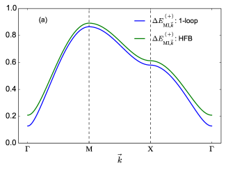
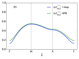
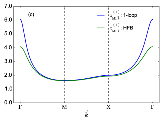
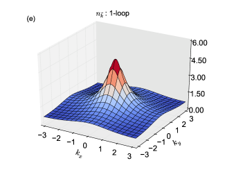
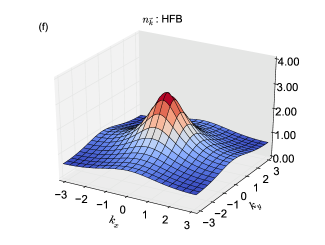
Figure 5: (Color online) Comparisons between the 1-loop and the HFB equilibrium solution in the Mott-insulating phase. The parameters used were $d=2$, $N_{s}=1000^{2}$, $\mu/U=0.42$, $J/U=0.04$, $\beta U=\infty$. (a) The particle excitation energy $\Delta E_{\text{MI},\vec{k}}^{\left(+\right)}$, (b) the hole excitation energy $\Delta E_{\text{MI},\vec{k}}^{\left(-\right)}$, (c) the particle spectral weight $z_{\text{MI},\vec{k}}^{\left(+\right)}$, (d) the hole spectral weight $z_{\text{MI},\vec{k}}^{\left(-\right)}$, (e) the quasi-momentum distribution $n_{\vec{k}}$ in the 1-loop approximation, (f) $n_{\vec{k}}$ in the HFB approximation. Note that $\Gamma=\left(0,0\right)$, $M=\left(\pi,\pi\right)$, and $X=\left(\pi,0\right)$.

One way to account for the differences in the spectral weights is to consider how well each solution scheme approximates the phase boundary between Mott insulating and superfluid phases. In Fig. 6 we compare the mean-field (MF) and HFB approximations of the phase boundary along with the exact calculation. Figure 6 clearly shows that there is significant quantitative improvement in the phase boundary calculation when going from the MF level to the HFB level. Moreover, in 1 dimension, where the MF approximation is expected to be poor, we have a clear qualitative improvement in the phase boundary calculation. The closer we are to the phase boundary (in the Mott-insulator phase), the sharper the $\vec{k}=0$ peak is in $n_{\vec{k}}$. Since the MF approximation always underestimates the location of the phase boundary more than the HFB approximation, the 1-loop approximation – which uses the MF approximation of $\phi$ – will wrongly predict a sharper peak as compared to that in the HFB case. Equivalently, the 1-loop approximation will always overestimate the values of the spectral weights in the neighbourhood of $\vec{k}=0$.

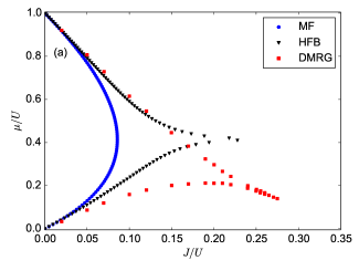
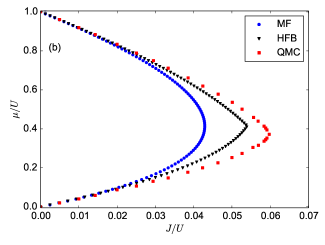
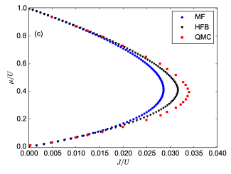
Figure 6: (Color online) Comparisons between the MF and the HFB approximations of the phase boundary along with the exact solution for $\beta U=\infty$: (a) $d=1$, (b) $d=2$, (c) $d=3$. The exact data was taken from Fig. 3 in Ref. [86] for $d=1$, Fig. 1 in Ref. [87] for $d=2$, and Fig. 3 in Ref. [88] for $d=3$.

Another way to assess the accuracy of the two approximation schemes in the Mott-insulating phase is to look at the average particle density $n$ [Eq. (149)]. In the Mott-insulating phase, $n=\left\lceil\mu/U\right\rceil$. For the same parameter values mentioned above, we have

$$n \approx 1.22,\qquad\text{(1-loop)},$$ (153)

$$n \approx 1.08,\qquad\text{(HFB)},$$ (154)

$$n = 1.00,\qquad\text{(exact)},$$ (155)

where we see that the HFB approximation yields a significant improvement as compared to the 1-loop approximation.

4.2 Superfluid phase

In the superfluid phase, $\phi$ and $\Sigma_{\vec{k}}^{22,\left(R,A\right)}$ are non-zero, hence we must use the full form of Eq. (135). We begin by calculating $\phi$ from Eqs. (126) and (111). Without loss of generality, we can assume that $\phi$ is real which further implies that the quantities $iG_{\vec{r}=\mathbf{0}}^{11,\left(K\right)}\left(s^{\prime}=0\right)$ and $iG_{\vec{r}=\mathbf{0}}^{22,\left(K\right)}\left(s^{\prime}=0\right)$ are real. Based on these assumptions we obtain

$$\phi = \sqrt{\frac{\left\{\mathcal{G}^{12,\left(R\right)}\left(\omega^{\prime}=0\right)\right\}^{-1}+2dJ}{u_{1}}-2\left(n-n_{0}\right)-\frac{1}{2}\left\{iG_{\vec{r}=\mathbf{0}}^{22,\left(K\right)}\left(s^{\prime}=0\right)\right\}}.$$ (156)

As is clear from Eq. (156) the mean field $\phi$ needs to be solved self-consistently along with the full propagator $G$. We now calculate $G^{\left(R\right)}$. Starting from Eq. (135), one can show that

$$G_{\vec{k}}^{12,\left(R\right)}\left(\omega\right) = \frac{\left(\omega^{+}+\Delta E_{\text{MI},\vec{k}}^{\left(+\right)}\right)\left(\omega^{+}-\Delta E_{\text{MI},\vec{k}}^{\left(-\right)}\right)\left(\omega^{+}+\left\{U+\mu\right\}\right)}{\left(\omega^{+}-\Delta E_{\text{SF},\vec{k}}^{\left(1\right)}\right)\left(\omega^{+}+\Delta E_{\text{SF},\vec{k}}^{\left(1\right)}\right)\left(\omega^{+}-\Delta E_{\text{SF},\vec{k}}^{\left(2\right)}\right)\left(\omega^{+}+\Delta E_{\text{SF},\vec{k}}^{\left(2\right)}\right)},$$ (157)

where

$$\Delta E_{\text{SF},\vec{k}}^{\left(s\right)} = \sqrt{\frac{-\tilde{B}_{\vec{k}}-\left(-1\right)^{s}\sqrt{\left(\tilde{B}_{\vec{k}}\right)^{2}-4\tilde{C}_{\vec{k}}}}{2}},$$ (158)

$$\tilde{B}_{\vec{k}} = \left|\Sigma_{\vec{k}}^{22,\left(R\right)}\right|^{2}-\left(\Delta E_{\text{MI},\vec{k}}^{\left(+\right)}\right)^{2}-\left(\Delta E_{\text{MI},\vec{k}}^{\left(-\right)}\right)^{2},$$ (159)

$$\tilde{C}_{\vec{k}} = \left(\Delta E_{\text{MI},\vec{k}}^{\left(+\right)}\Delta E_{\text{MI},\vec{k}}^{\left(-\right)}\right)^{2}-\left(U+\mu\right)^{2}\left|\Sigma_{\vec{k}}^{22,\left(R\right)}\right|^{2},$$ (160)

In a moment we will show that the $\Delta E_{\text{SF},\vec{k}}^{\left(s\right)}$ are the excitation energies in the SF phase. Before doing so, it is worth commenting on our approximation for the self energy in the superfluid phase. In E we show that in the full HFB approximation the excitation spectrum is not gapless, violating Goldstone’s Theorem, whereas if we ignore contributions from the anomalous Keldysh Green’s function $iG_{\vec{r}=0}^{22,\left(K\right)}\left(s^{\prime}=0\right)$ there is a gapless spectrum. The latter scheme is called the HFB-Popov (HFBP) approximation [89]. Thus in the HFBP approximation we have

$$\Sigma_{\vec{k}}^{22,\left(R\right)} = u_{1}\left(\phi\right)^{2},$$ (161)

$$\phi = \sqrt{\frac{\left\{\mathcal{G}^{12,\left(R\right)}\left(\omega^{\prime}=0\right)\right\}^{-1}+2dJ}{u_{1}}-2\left(n-n_{0}\right)}.$$ (162)

The HFBP approximation is most accurate for values of the chemical potential away from integer values which is evident from the fact that $G_{\vec{k}}^{22,\left(R\right)}\left(\omega\right)$ (and hence $G_{\vec{r}=\mathbf{0}}^{22,\left(K\right)}\left(s^{\prime}=0\right)$) is proportional to $\Sigma_{\vec{k}}^{22,\left(R\right)}$, which in turn is proportional to $u_{1}$, which is small for values of the chemical potential away from integer values. Therefore $iG_{\vec{r}=\mathbf{0}}^{22,\left(K\right)}\left(s^{\prime}=0\right)$ ought to be smaller than the average particle density $n$ by a factor of $u_{1}$.

For the remainder of this section, we apply the HFBP approximation. Since the energy spectrum is gapless in this approximation, i.e. $\Delta E_{\text{SF},\vec{k}\to 0}^{\left(2\right)}\to 0$, care must be taken in calculating the spectral function from the retarded Green’s function. Hence we will break the calculations up into two cases: the general case $\vec{k}\neq 0$ and the special case $\vec{k}=0$. We start with the general case.

4.2.1 $\vec{k}\neq 0$

When $\vec{k}\neq 0$, we can derive the spectral function from the retarded Green’s function as we did above in Sec. 4.1 using the Sokhotski-Plemelj formula as we did in the MI case [Eq. (147)]

$$G_{\vec{k}}^{12,\left(\rho\right)}\left(\omega\right) = 2\pi\left\{z_{\text{SF},\vec{k}}^{\left(1,+\right)}\delta\left(\omega-\Delta E_{\text{SF},\vec{k}}^{\left(1\right)}\right)-z_{\text{SF},\vec{k}}^{\left(1,-\right)}\delta\left(\omega+\Delta E_{\text{SF},\vec{k}}^{\left(1\right)}\right)\right.$$ (163)

$$\left.\qquad+z_{\text{SF},\vec{k}}^{\left(2,+\right)}\delta\left(\omega-\Delta E_{\text{SF},\vec{k}}^{\left(2\right)}\right)-z_{\text{SF},\vec{k}}^{\left(2,-\right)}\delta\left(\omega+\Delta E_{\text{SF},\vec{k}}^{\left(2\right)}\right)\right\},$$

where

$$z_{\text{SF},\vec{k}}^{\left(s,\pm\right)} = \left(-1\right)^{s+1}\frac{\left(\Delta E_{\text{SF},\vec{k}}^{\left(s\right)}\pm\Delta E_{\text{MI},\vec{k}}^{\left(+\right)}\right)\left(\Delta E_{\text{SF},\vec{k}}^{\left(s\right)}\mp\Delta E_{\text{MI},\vec{k}}^{\left(-\right)}\right)\left(\left\{U+\mu\right\}\pm\Delta E_{\text{SF},\vec{k}}^{\left(s\right)}\right)}{2\Delta E_{\text{SF},\vec{k}}^{\left(s\right)}\left[\left(\Delta E_{\text{SF},\vec{k}}^{\left(1\right)}\right)^{2}-\left(\Delta E_{\text{SF},\vec{k}}^{\left(2\right)}\right)^{2}\right]}.$$ (164)

It is clear from Eq. (163) that $\Delta E_{\text{SF},\vec{k}}^{\left(s\right)}$ and $z_{\text{SF},\vec{k}}^{\left(s,\pm\right)}$ are the excitation energies and spectral weights respectively. Moreover, for each branch the particle excitation energy is equal to the hole excitation energy. Using Eq. (128) we have for the Keldysh Green’s function

$$G_{\vec{k}}^{12,\left(K\right)}\left(\omega\right) = -2\pi i\left\{z_{\text{SF},\vec{k}}^{\left(1,+\right)}\delta\left(\omega-\Delta E_{\text{SF},\vec{k}}^{\left(1\right)}\right)+z_{\text{SF},\vec{k}}^{\left(1,-\right)}\delta\left(\omega+\Delta E_{\text{SF},\vec{k}}^{\left(1\right)}\right)\right.$$ (165)

$$\left.\qquad\qquad+z_{\text{SF},\vec{k}}^{\left(2,+\right)}\delta\left(\omega-\Delta E_{\text{SF},\vec{k}}^{\left(2\right)}\right)+z_{\text{SF},\vec{k}}^{\left(2,-\right)}\delta\left(\omega+\Delta E_{\text{SF},\vec{k}}^{\left(2\right)}\right)\right\}.$$

4.2.2 $\vec{k}=0$

In the zero-quasi-momentum case, $G_{\vec{k}}^{12,\left(K\right)}\left(\omega\right)$ becomes

$$G_{\vec{k}=0}^{12,\left(R\right)}\left(\omega\right) = \frac{\left(\omega^{+}+\Delta E_{\text{MI},\vec{k}=0}^{\left(+\right)}\right)\left(\omega^{+}-\Delta E_{\text{MI},\vec{k}=0}^{\left(-\right)}\right)\left(\omega^{+}+\left\{U+\mu\right\}\right)}{\left(\omega^{+}-\Delta E_{\text{SF},\vec{k}=0}^{\left(1\right)}\right)\left(\omega^{+}+\Delta E_{\text{SF},\vec{k}=0}^{\left(1\right)}\right)\left(\omega^{+}\right)^{2}}.$$ (166)

One cannot use the same Sokhotski-Plemelj formula as we did above in deriving the spectral function, instead one must used a generalized version of the formula

$$\frac{f\left(x\right)}{\left(x+i0^{\pm}-x_{0}\right)^{n}} = \mp i\pi f^{\left(n-1\right)}\left(x_{0}\right)\delta\left(x-x_{0}\right)+\Gamma\left(n\right)\mathcal{P}\left\{\frac{f\left(x\right)}{\left(x-x_{0}\right)^{n}}\right\}.$$ (167)

Doing so yields the following spectral function

$$G_{\vec{k}=0}^{12,\left(\rho\right)}\left(\omega\right) = 2\pi\left\{z_{\text{SF},\vec{k}=0}^{\left(1,+\right)}\delta\left(\omega-\Delta E_{\text{SF},\vec{k}=0}^{\left(1\right)}\right)-z_{\text{SF},\vec{k}=0}^{\left(1,-\right)}\delta\left(\omega+\Delta E_{\text{SF},\vec{k}=0}^{\left(1\right)}\right)\right.$$ (168)

$$\left.\qquad+\lim_{\vec{k}\to 0}\left[z_{\text{SF},\vec{k}}^{\left(2,+\right)}-z_{\text{SF},\vec{k}}^{\left(2,-\right)}\right]\delta\left(\omega\right)\right\},$$

where

$$\lim_{\vec{k}\to 0}\left[z_{\text{SF},\vec{k}}^{\left(2,+\right)}-z_{\text{SF},\vec{k}}^{\left(2,-\right)}\right] = \frac{\left(U+\mu\right)\left(\Delta E_{\text{MI},\vec{k}=0}^{\left(+\right)}-\Delta E_{\text{MI},\vec{k}=0}^{\left(-\right)}\right)-\Delta E_{\text{MI},\vec{k}=0}^{\left(+\right)}\Delta E_{\text{MI},\vec{k}=0}^{\left(-\right)}}{\left(\Delta E_{\text{SF},\vec{k}=0}^{\left(1\right)}\right)^{2}}.$$ (169)

In both $\vec{k}$ cases, $G_{\vec{k}}^{12,\left(\rho\right)}\left(\omega\right)$ is both properly normalized and signed [62].

In the case where $\vec{k}=0$, one needs to be careful when calculating $G_{\vec{k}=0}^{12,\left(K\right)}\left(\omega\right)$ as the FDT [Eq. (128)] is ill-defined for $\omega=0$. Fortunately, $G_{\vec{k}}^{12,\left(K\right)}\left(\omega\right)=0$ (see F for a proof). Therefore we have for $G_{\vec{k}=0}^{12,\left(K\right)}\left(\omega\right)$

$$G_{\vec{k}=0}^{12,\left(K\right)}\left(\omega=0\right) = 0,$$ (170)

$$G_{\vec{k}=0}^{12,\left(K\right)}\left(\omega\neq 0\right) = -2\pi i\left\{z_{\text{SF},\vec{k}}^{\left(1,+\right)}\delta\left(\omega-\Delta E_{\text{SF},\vec{k}}^{\left(1\right)}\right)+z_{\text{SF},\vec{k}}^{\left(1,-\right)}\delta\left(\omega+\Delta E_{\text{SF},\vec{k}}^{\left(1\right)}\right)\right\}.$$ (171)

4.2.3 Calculating $n_{\vec{k}}$ and $n$

One can calculate $n_{\vec{k}}$ from

$$n_{\vec{k}} = \frac{1}{2}\left\langle iG_{\vec{k}}^{12,\left(K\right)}\left(s^{\prime}=0\right)+2\left\{\left(2\pi\right)^{d}\delta_{\vec{k},\mathbf{0}}\right\}\left|\phi\right|^{2}-1\right\rangle,$$ (172)

where

$$iG_{\vec{k}}^{12,\left(K\right)}\left(t^{\prime}=0\right) = \begin{cases}z_{\text{SF},\vec{k}^{\prime}}^{\left(1,+\right)}+z_{\text{SF},\vec{k}^{\prime}}^{\left(1,-\right)}+z_{\text{SF},\vec{k}^{\prime}}^{\left(2,+\right)}+z_{\text{SF},\vec{k}^{\prime}}^{\left(2,-\right)}&\text{if }\vec{k}\neq 0\\ z_{\text{SF},\vec{k}}^{\left(1,+\right)}+z_{\text{SF},\vec{k}}^{\left(1,-\right)}&\text{if }\vec{k}=0\end{cases}.$$ (173)

And lastly, the average particle density $n$ is calculated using Eq. (149). Therefore, at the HFBP level, the system can be solved self-consistently as follows:

1. Make an initial guess for $n$.

2. Use $n$ to calculate $\phi$ via Eq. (156).

3. Use $n$ and $\phi$ to calculate $\Sigma_{\vec{k}}^{12,\left(R\right)}$ and $\Sigma_{\vec{k}}^{22,\left(R\right)}$ via Eqs. (130) and (161).

4. Use $\Sigma_{\vec{k}}^{12,\left(R\right)}$ to calculate $\Delta E_{\text{SF},\vec{k}}^{\left(s\right)}$ via Eqs. (140)–(142) and (158)–(160).

5. Use $\Delta E_{\text{SF},\vec{k}}^{\left(s\right)}$ to calculate $z_{\text{SF},\vec{k}}^{\left(s,\pm\right)}$ via Eqs. (164) and (169).

6. Use $z_{\text{SF},\vec{k}}^{\left(s,\pm\right)}$ to calculate $n_{k}$ via Eqs. (172) and (173).

7. Use $n_{\vec{k}}$ to recalculate $n$ via Eq. (149).

8. Repeat steps 2 to 7 until self-consistency is reached.

In Fig. 7, we compare the 1-loop and HFBP equilibrium solutions in the superfluid phase by calculating the excitation energies $\Delta E_{\text{SF},\vec{k}}^{\left(s\right)}$ and the spectral weights $z_{\text{SF},\vec{k}}^{\left(s,\pm\right)}$ for a square lattice system with $\mu/U=0.36$, $J/U=0.07$, and $\beta U=\infty$. The 1-loop solution amounts to approximating the self-energy by $\Sigma_{\vec{k}}^{12,\left(R\right)}=\epsilon_{\vec{k}}+2u_{1}\left|\phi\right|^{2}$ and $\Sigma_{\vec{k}}^{22,\left(R\right)}=u_{1}\left(\phi\right)^{2}$ in the superfluid phase. We see that there is little qualitative change in the excitation energies between the two approximations. Moreover, the spectral weights in the second branch $s=2$ change very little as well. We do observe appreciable differences in the spectral weights for the first branch $s=1$ in the long-wavelength limit, similar to the Mott-insulator case. As was argued for in the Mott-insulator case, since the HFBP calculation yields a more accurate phase boundary, we believe this method will also yield a more accurate result for $z_{\text{SF},\vec{k}}^{\left(1,\pm\right)}$ in the long-wavelength limit as compared to the 1-loop result.

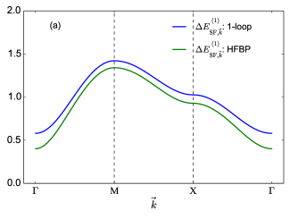
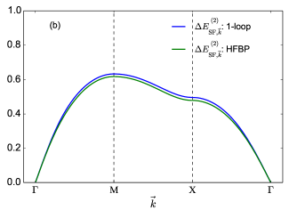
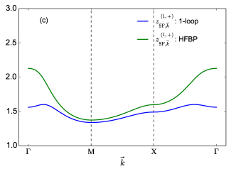
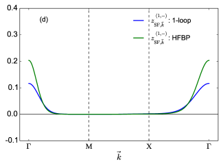
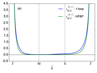
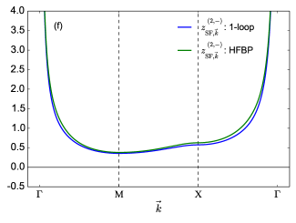
Figure 7: (Color online) Comparisons between the 1-loop and the HFBP equilibrium solution in the superfluid phase. The parameters used were $d=2$, $N_{s}=1000^{2}$, $\mu/U=0.36$, $J/U=0.07$, $\beta U=\infty$. (a) The first particle/hole excitation energy branch $\Delta E_{\text{SF},\vec{k}}^{\left(1\right)}$, (b) the second particle/hole excitation energy branch $\Delta E_{\text{SF},\vec{k}}^{\left(2\right)}$, (c) the particle spectral weight $z_{\text{SF},\vec{k}}^{\left(1,+\right)}$for the first branch, (d) the hole spectral weight $z_{\text{SF},\vec{k}}^{\left(1,-\right)}$for the first branch, (e) the particle spectral weight $z_{\text{SF},\vec{k}}^{\left(2,+\right)}$for the second branch, (f) the hole spectral weight $z_{\text{SF},\vec{k}}^{\left(2,-\right)}$for the second branch. Note that $\Gamma=\left(0,0\right)$, $M=\left(\pi,\pi\right)$, and $X=\left(\pi,0\right)$.

4.3 Phase boundary

To calculate the phase boundary, we make a slight modification to our solution scheme for the MI phase. The modification comes from the extra step of calculating the critical hopping $J_{c}$. Consider again the $\phi$-equation Eq. (156). At the boundary, $\phi=G_{\vec{r}=\mathbf{0}}^{22,\left(K\right)}\left(s^{\prime}=0\right)=0$. Solving for $J$ we get

$$J_{c} = \frac{1}{2d}\left\{2u_{1}\left(n-n_{0}\right)-\left\{\mathcal{G}^{12,\left(R\right)}\left(\omega^{\prime}=0\right)\right\}^{-1}\right\}.$$ (174)

With this established, we can outline the phase boundary solution as follows

1. Make an initial guess for the average particle density $n$

2. Use $n$ to calculate the hopping $J_{c}$, see Eq. (174)

3. Use $n$ and $J_{c}$ to calculate the self-energy $\Sigma_{\vec{k}}^{12,\left(R\right)}$, see Eq. (130)

4. Use $\Sigma_{\vec{k}}^{12,\left(R\right)}$ to calculate $\Delta E_{\text{MI},\vec{k}}^{\left(\pm\right)}$ via Eqs. (140)–(142).

5. Use $\Delta E_{\text{MI},\vec{k}}^{\left(\pm\right)}$ to calculate $z_{\text{MI},\vec{k}}^{\left(\pm\right)}$ via Eq. (143).

6. Use $z_{\text{MI},\vec{k}}^{\left(\pm\right)}$ to calculate $n_{k}$ via Eq. (152).

7. Use $n_{\vec{k}}$ to recalculate $n$ via Eq. (149).

8. Repeat steps 2 to 7 until self-consistency is reached.

This calculation ends up reproducing the phase boundary found from the Mott insulating side since the anomalous Green’s functions vanish at the phase boundary.

5 Discussion and Conclusions

The ability to address single sites in cold atom experiments [11] has allowed for experimental exploration of spatio-temporal correlations in the BHM [49]. This has led to theoretical investigations of these correlations in both one [48] and higher dimensions [46, 51, 59, 61] in the presence of a quench. In dimensions higher than one, where numerical approaches are limited, a theoretical challenge has been to develop a framework which can treat correlations in both the superfluid and Mott insulating phases over the course of a quench. An important result in this paper is that we have developed a formalism that allows for the description of the space and time dependence of correlations in both phases during a quench. The specific approach we took was to derive a 2PI effective action for the BHM using the contour-time technique building on the 1PI real-time strong-coupling theory developed in Ref. [31] which generalized the imaginary-time theory developed in Ref. [62]. From this 2PI effective action we were able to derive equations of motion that treat the superfluid order parameter and the full two-point Green’s functions on equal footing. We emphasise that our formalism is applicable even in the limit of low occupation number per site.

Even at the level of the 1PI real-time theory, the quartic coupling becomes non-local in time, which in the 2PI theory leads to complicated expressions in the equations of motion, involving up to four time integrals, even at the first order in the interaction vertices. We showed that by taking a low frequency approximation, this complexity can be reduced to at most a single time integral. The equations of motion obtained at this point are somewhat similar to previous 2PI studies of the out of equilibrium dynamics of interacting bosons [63, 75, 90, 91, 92, 93]. However, in contrast to these previous studies, the equations of motion we obtain are a series of integral equations rather than integro-differential equations.

We showed that taking a HFB(P) approximation of the 2PI effective action yields significant improvements to the calculation of the particle density and phase boundary when compared to the 1-loop approximation considered in Ref. [62]. Our results also suggest that the HFB(P) approximation gives a better account of the spectral weights in the long-wavelength limit. These improvements in the equilibrium case suggest that our formalism should be suitable for accurately describing spatio-temporal correlations in nonequilibrium scenarios.

The space and time dependence of correlations after a quantum quench give insight into the propagation of excitations generated by that quench, and hence we hope that the formalism we have developed here will allow further theoretical investigation of the excitations after quenches in the BHM, to complement experimental efforts in the same direction. In future work we plan to investigate a broad range of quench protocols, including quenches in the Mott phase where one can study the light-cone-like spreading of single-particle correlations. Other quench protocols of interests are those beginning in the superfluid phase and then ending in the Mott phase. In such scenarios, one may be interested in studying for example the possibility of aging-like phenomena. Lastly, we plan to investigate generalizations such as the inclusion of a harmonic trap, coupling to a bath [71, 94] or a multicomponent BHM.

Appendix A Deriving the strong-coupling effective theory

In this appendix, we briefly review the derivation of the effective theory for the BHM [Eq. 52] and make note of some minor mistakes in Ref. [31] (all of these mistakes relate to mislabelling of Keldysh indices – numerical results in Ref. [31] are unaffected). The derivation given in Ref. [31] was for the case of the Schwinger-Keldysh contour, here we extend the derivation to the more general contour illustrated in Fig. 1. We make use of the compact notation introduced in Section 2.6 when it is helpful.

We start with the generating functional $\mathcal{Z}\left[f\right]$

$$\mathcal{Z}\left[f\right] = \int\left[\mathcal{D}a^{a}\right]e^{\frac{i}{2!}\sum_{\vec{r}_{1}\vec{r}_{2}}\left(2J_{\vec{r}_{1}\vec{r}_{2},\tau_{1}\tau_{2}}^{\overline{a_{1}}\overline{a_{2}}}\right)a_{\vec{r}_{1},\tau_{1}}^{a_{1}}a_{\vec{r}_{2},\tau_{2}}^{a_{2}}+iS_{0}\left[a\right]+iS_{f}\left[a\right]},$$ (175)

where $J_{\vec{r}_{1}\vec{r}_{2},\tau_{1}\tau_{2}}^{a_{1}a_{2}}$ is defined in Eq. (65), $S_{f}\left[a\right]$ is defined in Eq. (50), and

$$S_{0} = \frac{1}{2}\int_{0}^{s_{\alpha_{1}\alpha_{2}}^{f}}ds\sum_{\vec{r}}\left[a_{\vec{r},\alpha_{1}}^{a_{1}}\left(s\right)\left(\left[\tau^{0}\right]_{\alpha_{1}\alpha_{3}}^{\dagger}\tau_{\alpha_{3}\alpha_{2}}^{1}\sigma_{2}^{a_{1}a_{2}}\partial_{s}\right)a_{\vec{r},\alpha_{2}}^{a_{2}}\left(s\right)\right]+S_{U}\left[a\right],$$ (176)

is the atomic part of the BHM action. Next we introduce an auxiliary field $\psi$ via a complex Hubbard-Stratonovich transformation [62, 31] so the generating functional $\mathcal{Z}\left[f\right]$ takes the form

$$\mathcal{Z}\left[f\right] = \int\left[\mathcal{D}\psi^{a}\right]\int\left[\mathcal{D}a^{a}\right]e^{-\frac{i}{2!}\sum_{\vec{r}_{1}\vec{r}_{2}}\left(\frac{1}{2}\left[J^{-1}\right]_{\vec{r}_{1}\vec{r}_{2},\tau_{1}\tau_{2}}^{\overline{a_{1}}\overline{a_{2}}}\right)\psi_{\vec{r}_{1},\tau_{1}}^{a_{1}}\psi_{\vec{r}_{2},\tau_{2}}^{a_{2}}-iS_{\psi}\left[a\right]+iS_{0}\left[a\right]+iS_{f}\left[a\right]},$$ (177)

where

$$S_{\psi}\left[a\right] = \sum_{\vec{r}}\psi_{\vec{r},\tau}^{\overline{a}}a_{\vec{r},\tau}^{a}.$$ (178)

We can eliminate the $iS_{f}$ term in Eq. (177) by making a field substitution, $\psi_{\vec{r},\tau}^{a}\to-\psi_{\vec{r},\tau}^{a}+f_{\vec{r},\tau}^{a}$, which gives

$$\mathcal{Z}\left[f\right] = \int\left[\mathcal{D}\psi^{a}\right]e^{-\frac{i}{2!}\sum_{\vec{r}_{1}\vec{r}_{2}}\left(\frac{1}{2}\left[J^{-1}\right]_{\vec{r}_{1}\vec{r}_{2},\tau_{1}\tau_{2}}^{\overline{a_{1}}\overline{a_{2}}}\right)\left(\psi_{\vec{r}_{1},\tau_{1}}^{a_{1}}-f_{\vec{r}_{1},\tau_{1}}^{a_{1}}\right)\left(\psi_{\vec{r}_{2},\tau_{2}}^{a_{2}}-f_{\vec{r}_{2},\tau_{2}}^{a_{2}}\right)+iW_{0}\left[\psi\right]},$$ (179)

where

$$e^{iW_{0}\left[\psi\right]} = \frac{1}{\mathcal{N}_{0}}\int\left[\mathcal{D}a^{a}\right]e^{iS_{0}\left[a\right]+iS_{\psi}\left[a\right]},$$ (180)

$$\mathcal{N}_{0} = \int\left[\mathcal{D}a^{a}\right]e^{iS_{0}\left[a\right]},$$ (181)

In obtaining Eq. (179) we absorbed a factor of $\mathcal{N}_{0}$ into the $\psi$-measure $\int\left[\mathcal{D}\psi^{a}\right]$. Comparing Eq. (180) with Eq. (22), we see that $W_{0}\left[\psi\right]$ is the generator of atomic CCOGFs $\mathcal{G}^{c}$ for the bosonic field $a$. The CCOGFs considered explicitly by the authors in Ref. [31] were

$$\mathcal{G}_{\vec{r},\alpha_{1}\ldots\alpha_{n}\alpha_{1}^{\prime}\ldots\alpha_{n}^{\prime}}^{n,c}\left(s_{1},\ldots,s_{n},s_{1}^{\prime}\ldots,s_{n}^{\prime}\right)$$

$$\quad\equiv\mathcal{G}_{\underbrace{\vec{r}\ldots\vec{r}}_{2n\text{ terms}},\alpha_{1}\ldots\alpha_{n}\alpha_{1}^{\prime}\ldots\alpha_{n}^{\prime}}^{\overbrace{1\ldots 1}^{n\text{ terms}}\overbrace{2\ldots 2}^{n\text{ terms}},c}\left(s_{1},\ldots,s_{n},s_{1}^{\prime}\ldots,s_{n}^{\prime}\right)$$

$$\quad=\left(-1\right)\left(\left[\tau^{1}\right]_{\alpha_{1}\alpha_{1}^{\prime\prime}}^{\dagger}\ldots\left[\tau^{1}\right]_{\alpha_{n}\alpha_{n}^{\prime\prime}}^{\dagger}\left[\tau^{1}\right]_{\alpha_{1}^{\prime}\alpha_{1}^{\prime\prime\prime}}^{\dagger}\ldots\left[\tau^{1}\right]_{\alpha_{n}^{\prime}\alpha_{n}^{\prime\prime\prime}}^{\dagger}\right)$$

$$\quad\phantom{=}\quad\times\left.\frac{\delta^{2n}W_{0}\left[\psi\right]}{\delta f_{\vec{r},\alpha_{1}^{\prime\prime}}^{*}\left(s_{1}\right)\ldots\delta f_{\vec{r},\alpha_{n}^{\prime\prime}}^{*}\left(s_{n}\right)\delta f_{\vec{r},\alpha_{1}^{\prime\prime\prime}}\left(s_{1}^{\prime}\right)\ldots\delta f_{\vec{r},\alpha_{n}^{\prime\prime\prime}}\left(s_{n}^{\prime}\right)}\right|_{\psi=0}$$

$$\quad=i\left(-1\right)^{n}\left\langle a_{\vec{r},\alpha_{1}}\left(s_{1}\right)\ldots a_{\vec{r},\alpha_{n}}\left(s_{n}\right)a_{\vec{r},\alpha_{1}^{\prime}}^{*}\left(s_{1}^{\prime}\right)\ldots a_{\vec{r},\alpha_{n}^{\prime}}^{*}\left(s_{n}^{\prime}\right)\right\rangle_{S_{0}}^{c}.$$ (182)

Note that Eq. (182) corrects Eq. (6) in Ref. [31]. Moreover, note that for the uniform BHM as considered here, the atomic CCOGFs are independent of site index, and so we drop these indices when they do not affect the clarity of the exposition in this paper.

Inverting Eq. (25), with $G^{c}\to\mathcal{G}^{c}$, we may rewrite $W_{0}$ as

$$W_{0}\left[\psi\right] = -\sum_{\vec{r}}\sum_{n=1}^{\infty}\frac{1}{\left(2n\right)!}\mathcal{G}_{\tau_{1}\ldots\tau_{2n}}^{\overline{a_{1}}\ldots\overline{a_{2n}},c}\psi_{\vec{r},\tau_{1}}^{a_{1}}\ldots\psi_{\vec{r},\tau_{2n}}^{a_{2n}},$$ (183)

which corrects Eq. (7) in Ref. [31] by a factor of $-\left(-1\right)^{n}$, and so

$$e^{iW_{0}\left[\psi\right]} = e^{i\sum_{n=1}^{\infty}S_{\text{int}}^{n}\left[\psi\right]},$$ (184)

where

$$S_{\text{int}}^{n}\left[\psi\right] = -\sum_{\vec{r}}\frac{1}{\left(2n\right)!}\mathcal{G}_{\tau_{1}\ldots\tau_{2n}}^{\overline{a_{1}}\ldots\overline{a_{2n}},c}\psi_{\vec{r},\tau_{1}}^{a_{1}}\ldots\psi_{\vec{r},\tau_{2n}}^{a_{2n}},$$ (185)

which corrects Eq. (8) in Ref. [31] by the same factor of $-\left(-1\right)^{n}$.

Truncating $W_{0}\left[\psi\right]$ to quartic order in the $\psi$ fields and setting the source currents $f$ to zero in Eq. (179), the action from Eq. (179) is found to be

$$S_{\text{eff}}\left[\psi\right] = -\frac{1}{2!}\sum_{\vec{r}_{1}\vec{r}_{2}}\left(\frac{1}{2}\left[J^{-1}\right]_{\vec{r}_{1}\vec{r}_{2},\tau_{1}\tau_{2}}^{\overline{a_{1}}\overline{a_{2}}}+\mathcal{G}_{\vec{r}_{1}\vec{r}_{2},\tau_{1}\tau_{2}}^{\overline{a_{1}}\overline{a_{2}},c}\right)\psi_{\vec{r}_{1},\tau_{1}}^{a_{1}}\psi_{\vec{r}_{2},\tau_{2}}^{a_{2}}$$ (186)

$$-\frac{1}{4!}\sum_{\vec{r}}\mathcal{G}_{\tau_{1}\tau_{2}\tau_{3}\tau_{4}}^{\overline{a_{1}}\overline{a_{2}}\overline{a_{3}}\overline{a_{4}},c}\psi_{\vec{r},\tau_{1}}^{a_{1}}\psi_{\vec{r},\tau_{2}}^{a_{2}}\psi_{\vec{r},\tau_{3}}^{a_{3}}\psi_{\vec{r},\tau_{4}}^{a_{4}}.$$

As pointed out in Ref. [62], the quadratic terms in the equilibrium action of the form in Eq. (186) allow one to calculate the mean-field phase boundary, however it yields an unphysical excitation spectrum in the superfluid regime. This issue is circumvented by performing a second Hubbard-Stratonovich transformation [62, 31]. Starting from Eq. (179) (keeping the source currents $f$ this time), we introduce a second field $z$ such that

$$\mathcal{Z}\left[f\right] = \int\left[\mathcal{D}z^{a}\right]e^{\frac{i}{2!}\sum_{\vec{r}_{1}\vec{r}_{2}}\left(2J_{\vec{r}_{1}\vec{r}_{2},\tau_{1}\tau_{2}}^{\overline{a_{1}}\overline{a_{2}}}\right)z_{\vec{r}_{1},\tau_{1}}^{a_{1}}z_{\vec{r}_{2},\tau_{2}}^{a_{2}}+i\widetilde{W}\left[z\right]+iS_{f}\left[z\right]},$$ (187)

where

$$S_{f}\left[z\right] = \sum_{\vec{r}}f_{\vec{r},\tau}^{\overline{a}}z_{\vec{r},\tau}^{a},$$ (188)

$$e^{i\widetilde{W}\left[z\right]} = \frac{1}{\mathcal{N}_{\psi}}\int\left[\mathcal{D}\psi^{a}\right]e^{iW_{0}\left[a\right]+iS_{z}\left[\psi\right]},$$ (189)

$$\mathcal{N}_{\psi} = \int\left[\mathcal{D}\psi^{a}\right]e^{iS_{\text{int}}^{1}\left[\psi\right]},$$ (190)

$$S_{z}\left[\psi\right] = \sum_{\vec{r}}z_{\vec{r},\tau}^{\overline{a}}\psi_{\vec{r},\tau}^{a}.$$ (191)

By comparing Eq. (187) to Eq. (22), we can see that the COGFs of the $z$ field generated by $\mathcal{Z}\left[f\right]$ are identical to those of the bosonic field $a$. The last step is to perform a cumulant expansion of $\widetilde{W}\left[z\right]$ [31, 62, 95]. Upon doing this, we can write the generating functional $\mathcal{Z}\left[f\right]$ as

$$\mathcal{Z}\left[f\right] = \int\left[\mathcal{D}z^{a}\right]e^{iS_{\text{BHM}}\left[z\right]+iS_{f}\left[z\right]},$$ (192)

where $S_{\text{BHM}}\left[z\right]$ is given by

$$S_{\text{BHM}}\left[z\right] = \frac{1}{2!}\sum_{\vec{r}_{1}\vec{r}_{2}}\left(2J_{\vec{r}_{1}\vec{r}_{2},\tau_{1}\tau_{2}}^{\overline{a_{1}}\overline{a_{2}}}+\left[\mathcal{G}^{-1}\right]_{\vec{r}_{1}\vec{r}_{2},\tau_{1}\tau_{2}}^{\overline{a_{1}}\overline{a_{2}},c}+\delta_{\vec{r}_{1}\vec{r}_{2}}\tilde{u}_{\tau_{1}\tau_{2}}^{\overline{a_{1}}\overline{a_{2}}}\right)z_{\vec{r}_{1},\tau_{1}}^{a_{1}}z_{\vec{r}_{2},\tau_{2}}^{a_{2}}$$ (193)

$$+\sum_{\vec{r}}\sum_{n=2}^{\infty}\frac{1}{\left(2n\right)!}\left(u_{\tau_{1}\ldots\tau_{2n}}^{\overline{a_{1}}\ldots\overline{a_{2n}}}+\tilde{u}_{\tau_{1}\ldots\tau_{2n}}^{\overline{a_{1}}\ldots\overline{a_{2n}}}\right)z_{\vec{r},\tau_{1}}^{a_{1}}\ldots z_{\vec{r},\tau_{2n}}^{a_{2n}},$$

with

$$u_{\tau_{1}\ldots\tau_{2n}}^{a_{1}\ldots a_{2n}} = -\prod_{m=1}^{n}\left(\left[\mathcal{G}^{-1}\right]_{\tau_{2m-1}\tau_{2m-1}^{\prime}}^{a_{2m-1}a_{2m-1}^{\prime},c}\left[\mathcal{G}^{-1}\right]_{\tau_{2m}\tau_{2m}^{\prime}}^{a_{2m}a_{2m}^{\prime},c}\right)\mathcal{G}_{\tau_{1}\ldots\tau_{2n}}^{\overline{a_{1}}\ldots\overline{a_{2n}},c},$$ (194)

and the $\tilde{u}$ vertices contain an infinite set of “anomalous” diagrams, i.e. diagrams that contain internal inverse bare propagator lines. Such diagrams have no physical meaning and should not contribute to the physical quantities [95]. It should be noted that in addition to the physical diagrams, the $u$ vertices also generate “anomalous” terms. In B, we show that these anomalous terms cancel one another out when calculating the superfluid order parameter $\phi$ and the full two-point CCOGF. That being said, the action in Eq. (193) contains an infinite sum, therefore one will eventually have to truncate said action which will ultimately lead to only certain subclasses of “anomalous” terms cancelling out.

In this paper, we truncate the action to quartic order in the $z$ fields

$$S_{\text{BHM}}\left[z\right] = \frac{1}{2!}\sum_{\vec{r}_{1}\vec{r}_{2}}\left(2J_{\vec{r}_{1}\vec{r}_{2},\tau_{1}\tau_{2}}^{\overline{a_{1}}\overline{a_{2}}}+\left[\mathcal{G}^{-1}\right]_{\vec{r}_{1}\vec{r}_{2},\tau_{1}\tau_{2}}^{\overline{a_{1}}\overline{a_{2}},c}+\delta_{\vec{r}_{1}\vec{r}_{2}}\tilde{u}_{\tau_{1}\tau_{2}}^{\overline{a_{1}}\overline{a_{2}}}\right)z_{\vec{r}_{1},\tau_{1}}^{a_{1}}z_{\vec{r}_{2},\tau_{2}}^{a_{2}}$$ (195)

$$+\sum_{\vec{r}}\frac{1}{4!}\left(u_{\tau_{1}\tau_{2}\tau_{3}\tau_{4}}^{\overline{a_{1}}\overline{a_{2}}\overline{a_{3}}\overline{a_{4}}}+\tilde{u}_{\tau_{1}\tau_{2}\tau_{3}\tau_{4}}^{\overline{a_{1}}\overline{a_{2}}\overline{a_{3}}\overline{a_{4}}}\right)z_{\vec{r},\tau_{1}}^{a_{1}}z_{\vec{r},\tau_{2}}^{a_{2}}z_{\vec{r},\tau_{3}}^{a_{3}}z_{\vec{r},\tau_{4}}^{a_{4}},$$

where we approximate $\tilde{u}^{\left(2\right)}$ by

$$\tilde{u}_{\tau_{1}\tau_{2}}^{a_{1}a_{2}} = -\frac{1}{2!}u_{\tau_{1}\tau_{2}\tau_{3}\tau_{4}}^{a_{1}a_{2}a_{3}a_{4},c}\left(i\mathcal{G}_{\tau_{3}\tau_{4}}^{\overline{a_{3}}\overline{a_{4}},c}\right),$$ (196)

and neglect any contributions from $\tilde{u}^{\left(4\right)}$. In Refs. [62, 31], all $\tilde{u}$ terms were neglected. By including the $\tilde{u}$ term given in Eq. (196), one obtains equations of motion which are accurate to first order in $\mathcal{G}^{\left(4\right),c}$, which is not the case in Refs. [62, 31]. Lastly, we stress that this approach leads to a strong-coupling theory that is not simply an expansion order by order in $J/U$.

Appendix B Cancellation of anomalous diagrams

In this appendix, we show that the anomalous terms introduced in A do not contribute when calculating the mean field $\phi$ and the two-point CCOGF $G^{c}$ of the original field $a$. For the sake of economy in writing, we adopt the notation introduced in Section 2.6 and condense it even further such that

$$X_{x_{1}\ldots x_{n}} \equiv X_{\vec{r}_{1}\ldots\vec{r}_{n},\tau_{1}\ldots\tau_{n}}^{a_{1}\ldots a_{n}},$$ (197)

$$X_{x}Y_{x} = \sum_{\vec{r}}X_{\vec{r},\tau}^{a}Y_{\vec{r},\tau}^{\overline{a}}.$$ (198)

We start with Eq. (177)

$$\mathcal{Z}\left[f\right] = \int\left[\mathcal{D}\psi^{a}\right]\int\left[\mathcal{D}a^{a}\right]e^{-\frac{i}{2!}\left(\frac{1}{2}\left[J^{-1}\right]_{x_{1}x_{2}}\right)\psi_{x_{1}}\psi_{x_{2}}-iS_{\psi}\left[a\right]+iS_{0}\left[a\right]+iS_{f}\left[a\right]}$$ (199)

$$= \int\left[\mathcal{D}\psi^{a}\right]\int\left[\mathcal{D}a^{a}\right]e^{\frac{i}{2!}\left(-\frac{1}{2}\left[J^{-1}\right]_{x_{1}x_{2}}\right)\psi_{x_{1}}\psi_{x_{2}}}\left\langle e^{i\left(S_{\psi}\left[a\right]+S_{f}\left[a\right]\right)}\right\rangle_{S_{0}},$$

where we performed the field substitution $\psi_{x}\to-\psi_{x}$. We first establish a relationship between the expectation values of the $a$-field, $\phi_{x}$, and of the $\psi$-field, $\mathcal{V}_{x}$. To do this, we start by calculating $\phi_{x_{1}}=\left\langle a_{x_{1}}\right\rangle$ as follows

$$\phi_{x_{1}} = \left\langle a_{x_{1}}\right\rangle$$ (200)

$$= -i\lim_{f\to 0}\frac{1}{\mathcal{Z}\left[f\right]}\frac{\delta\mathcal{Z}\left[f\right]}{\delta f_{x_{1}}}$$

$$= -i\lim_{f\to 0}\frac{1}{\mathcal{Z}\left[f\right]}\int\left[\mathcal{D}\psi^{a}\right]e^{\frac{i}{2!}\left(-\frac{1}{2}\left[J^{-1}\right]_{x_{2}x_{3}}\right)\psi_{x_{2}}\psi_{x_{3}}}\frac{\delta}{\delta f_{x_{1}}}\left\{\left\langle e^{i\left(S_{\psi}\left[a\right]+S_{f}\left[a\right]\right)}\right\rangle_{S_{0}}\right\}$$

$$= -i\lim_{f\to 0}\frac{1}{\mathcal{Z}\left[f\right]}\int\left[\mathcal{D}\psi^{a}\right]e^{\frac{i}{2!}\left(-\frac{1}{2}\left[J^{-1}\right]_{x_{2}x_{3}}\right)\psi_{x_{2}}\psi_{x_{3}}}\frac{\delta}{\delta\psi_{x_{1}}}\left\{\left\langle e^{i\left(S_{\psi}\left[a\right]+S_{f}\left[a\right]\right)}\right\rangle_{S_{0}}\right\},$$

and then integrate by parts to get

$$= i\lim_{f\to 0}\frac{1}{\mathcal{Z}\left[f\right]}\int\left[\mathcal{D}\psi^{a}\right]\frac{\delta}{\delta\psi_{x_{1}}}\left\{e^{\frac{i}{2!}\left(-\frac{1}{2}\left[J^{-1}\right]_{x_{2}x_{3}}\right)\psi_{x_{2}}\psi_{x_{3}}}\right\}\left\langle e^{i\left(S_{\psi}\left[a\right]+S_{f}\left[a\right]\right)}\right\rangle_{S_{0}}$$ (201)

$$= \frac{1}{2}\left[J^{-1}\right]_{x_{1}x_{2}}\left(\lim_{f\to 0}\frac{1}{\mathcal{Z}\left[f\right]}\int\left[\mathcal{D}\psi^{a}\right]\psi_{x_{2}}e^{\frac{i}{2!}\left(-\frac{1}{2}\left[J^{-1}\right]_{x_{3}x_{4}}\right)\psi_{x_{3}}\psi_{x_{4}}+iW_{0}\left[\psi+f\right]}\right)$$

$$= \frac{1}{2}\left[J^{-1}\right]_{x_{1}x_{2}}\mathcal{V}_{x_{2}},$$

which establishes a relation between $\phi_{x}$ and $\mathcal{V}_{x}$. Note that

$$\frac{\delta}{\delta\Phi_{x}}\left(\ldots\right) \equiv \frac{\delta}{\delta\Phi_{\vec{r},\tau}^{\overline{a}}}\left(\ldots\right),$$ (202)

where $\Phi$ is some arbitrary field. By similar calculation, one can show that

$$G_{x_{1}x_{2}}^{c} = \frac{1}{2}\left[J^{-1}\right]_{x_{1}x_{2}}+\left(\frac{1}{2}\left[J^{-1}\right]_{x_{1}x_{3}}\right)\left(\frac{1}{2}\left[J^{-1}\right]_{x_{2}x_{4}}\right)\mathcal{V}_{x_{3}x_{4}}^{c},$$ (203)

where $\mathcal{V}_{x_{1}x_{2}}^{c}$ is the two-point CCGOF for the field $\psi$. Taking the inverses of the above relations yields

$$\mathcal{V}_{x_{1}} = \left(2J_{x_{1}x_{2}}\right)\phi_{x_{2}},$$ (204)

$$\mathcal{V}_{x_{1}x_{2}}^{c} = -\left(2J_{x_{1}x_{2}}\right)+\left(2J_{x_{1}x_{3}}\right)\left(2J_{x_{2}x_{4}}\right)G_{x_{3}x_{4}}^{c}.$$ (205)

We now use the $\psi$ theory to calculate the 2PI equations of motion for $\mathcal{V}_{x_{1}}$ and $\mathcal{V}_{x_{1}x_{2}}^{c}$. The action $S_{\text{aux}}\left[\psi\right]$ for the auxiliary field $\psi$ can be expressed as

$$S_{\text{aux}}\left[\psi\right] = \frac{1}{2!}\left(-\frac{1}{2}\left[J^{-1}\right]_{x_{1}x_{2}}\right)\psi_{x_{1}}\psi_{x_{2}}-\sum_{n=1}^{\infty}\frac{1}{\left(2n\right)!}\mathcal{G}_{x_{1}\ldots x_{2n}}^{c}\psi_{x_{1}}\ldots\psi_{x_{2n}},$$ (206)

and hence using this action in Eqs. (78) and (79) and rearranging terms, we obtain the following relations

$$\mathcal{V}_{x_{1}} = -\left(2J_{x_{1}x_{2}}\right)\mathcal{G}_{x_{2}x_{3}}^{c}\mathcal{V}_{x_{3}}$$ (207)

$$-\left(2J_{x_{1}x_{2}}\right)\sum_{n=2}^{\infty}\frac{1}{\left(2n-3\right)!}\mathcal{G}_{x_{2}x_{3}x_{4}x_{5}\ldots x_{2n+1}}^{c}$$

$$\phantom{-\left(2J_{x_{1}x_{2}}\right)\sum_{n=2}^{\infty}}\times\left\{\frac{1}{\left(2n-1\right)\left(2n-2\right)}\mathcal{V}_{x_{3}}\mathcal{V}_{x_{4}}+\frac{1}{2}\left(i\mathcal{V}_{x_{3}x_{4}}^{c}\right)\right\}\mathcal{V}_{x_{5}}\ldots\mathcal{V}_{x_{2n+1}}$$

$$+\left(2J_{x_{1}x_{2}}\right)\Xi_{x_{2}}\left[\mathcal{G}^{\left(2n\right),c},\mathcal{V}^{\left(1\right)},\mathcal{V}^{\left(2\right),c}\right],$$

$$\mathcal{V}_{x_{1}x_{2}}^{c} = -\left(2J_{x_{1}x_{2}}\right)-\left(2J_{x_{1}x_{3}}\right)\mathcal{G}_{x_{3}x_{4}}^{c}\mathcal{V}_{x_{4}x_{2}}^{c}$$ (208)

$$-\left(2J_{x_{1}x_{3}}\right)\left\{\sum_{n=2}^{\infty}\frac{1}{\left(2n-2\right)!}\mathcal{G}_{x_{3}x_{4}x_{5}\ldots x_{2n+2}}^{c}\mathcal{V}_{x_{5}}\ldots\mathcal{V}_{x_{2n+2}}\right\}\mathcal{V}_{x_{4}x_{2}}^{c}$$

$$-\left(2J_{x_{1}x_{3}}\right)\Sigma_{x_{3}x_{4}}^{\text{aux}}\left[\mathcal{G}^{\left(2n\right),c},\mathcal{V}^{\left(1\right)},\mathcal{V}^{\left(2\right),c}\right]\mathcal{V}_{x_{4}x_{2}}^{c},$$

where $\Xi$ and $\Sigma$ are obtained from the corresponding $\Gamma_{2}$. Next, we apply Eqs. (204) and (205) to obtain recursive expressions for $\phi$ and $G^{c}$

$$\phi_{x_{1}} = -\mathcal{G}_{x_{1}x_{2}}^{c}\left(2J_{x_{2}x_{2}^{\prime}}\right)\phi_{x_{2}^{\prime}}$$ (209)

$$-\sum_{n=2}^{\infty}\frac{1}{\left(2n-3\right)!}\mathcal{G}_{x_{1}x_{2}x_{3}x_{4}\ldots x_{2n}}^{c}\left\{\frac{1}{\left(2n-1\right)\left(2n-2\right)}\left(2J_{x_{2}x_{2}^{\prime}}\right)\left(2J_{x_{3}x_{3}^{\prime}}\right)\phi_{x_{2}^{\prime}}\phi_{x_{3}^{\prime}}\right.$$

$$\phantom{-\sum_{n=2}^{\infty}\frac{1}{\left(2n-3\right)!}\mathcal{G}_{x_{1}x_{2}x_{3}x_{4}\ldots x_{2n}}^{c}}\quad\left.+\frac{i}{2}\left[-\left(2J_{x_{2}x_{3}}\right)+\left(2J_{x_{2}x_{2}^{\prime}}\right)\left(2J_{x_{3}x_{3}^{\prime}}\right)G_{x_{2}^{\prime}x_{3}^{\prime}}^{c}\right]\right\}$$

$$\phantom{-\sum_{n=2}^{\infty}}\quad\times\left(2J_{x_{4}x_{4}^{\prime}}\right)\ldots\left(2J_{x_{2n}x_{2n}^{\prime}}\right)\phi_{x_{4}^{\prime}}\ldots\phi_{x_{2n}^{\prime}}$$

$$+\Xi_{x_{1}}\left[\mathcal{G}^{\left(2n\right),c},\left(2J_{xx^{\prime}}\right)\phi_{x^{\prime}},-\left(2J_{xy}\right)+\left(2J_{xx^{\prime}}\right)\left(2J_{yy^{\prime}}\right)G_{x^{\prime}y^{\prime}}^{c}\right],$$

$$G_{x_{1}x_{2}}^{c} = \left\{\mathcal{G}_{x_{1}x_{3}}^{c}+\sum_{n=2}^{\infty}\frac{1}{\left(2n-2\right)!}\mathcal{G}_{x_{1}x_{3}x_{4}\ldots x_{2n+1}}^{c}\left(2J_{x_{4}x_{4}^{\prime}}\phi_{x_{4}^{\prime}}\right)\ldots\left(2J_{x_{2n+1}x_{2n+1}^{\prime}}\phi_{x_{2n+1}^{\prime}}\right)\right.$$ (210)

$$\left.\quad+\Sigma_{x_{1}x_{3}}^{\text{aux}}\left[\mathcal{G}^{\left(2n\right),c},\left(2J_{xx^{\prime}}\right)\phi_{x^{\prime}},-\left(2J_{xy}\right)+\left(2J_{xx^{\prime}}\right)\left(2J_{yy^{\prime}}\right)G_{x^{\prime}y^{\prime}}^{c}\right]\right\}$$

$$\quad\times\left\{\delta_{x_{3}x_{2}}-\left(2J_{x_{3}x_{3}^{\prime}}\right)G_{x_{3}^{\prime}x_{2}}^{c}\right\}.$$

We now derive recursive relations for $\phi$ and $G^{c}$ by an alternative approach: we apply the 2PI approach to the theory of the $z$-fields, allowing for anomalous terms, which is given by Eq. (193) and written again here in compact form

$$S_{\text{BHM}} = \frac{1}{2!}\left(\left[\mathcal{G}^{-1}\right]_{x_{1}x_{2}}^{c}+\tilde{u}_{x_{1}x_{2}}\right)z_{x_{1}}z_{x_{2}}+\frac{1}{2!}\left(2J_{x_{1}x_{2}}\right)z_{x_{1}}z_{x_{2}}$$ (211)

$$+\sum_{n=2}^{\infty}\frac{1}{\left(2n\right)!}\left(u_{x_{1}\ldots x_{2n}}+\tilde{u}_{x_{1}\ldots x_{2n}}\right)z_{x_{1}}\ldots z_{x_{2n}}.$$

As noted in A, the Green’s functions for the $z$-fields are the same as those for the $a$-fields. Similarly to the calculations leading to the recursive relations $\mathcal{V}_{x_{1}}$ and $\mathcal{V}_{x_{1}x_{2}}^{c}$, we calculate the following recursive 2PI relations for $\phi$ and $G^{c}$

$$\phi_{x_{1}} = -\mathcal{G}_{x_{1}x_{2}}^{c}\left(2J_{x_{2}x_{3}}\right)\phi_{x_{3}}-\mathcal{G}_{x_{1}x_{2}}^{c}\tilde{u}_{x_{2}x_{3}}\phi_{x_{3}}$$ (212)

$$-\mathcal{G}_{x_{1}x_{2}}^{c}\sum_{n=2}^{\infty}\frac{1}{\left(2n-3\right)!}\left\{u_{x_{2}x_{3}x_{4}x_{5}\ldots x_{2n+1}}+\tilde{u}_{x_{2}x_{3}x_{4}x_{5}\ldots x_{2n+1}}\right\}$$

$$\phantom{-\mathcal{G}_{x_{1}x_{2}}^{c}\sum_{n=2}^{\infty}}\quad\times\left\{\frac{1}{\left(2n-1\right)\left(2n-2\right)}\phi_{x_{3}}\phi_{x_{4}}+\frac{i}{2}G_{x_{3}x_{4}}^{c}\right\}\phi_{x_{5}}\ldots\phi_{x_{2n+1}}$$

$$-\mathcal{G}_{x_{1}x_{2}}^{c}\Xi_{x_{2}}\left[-u^{\left(2n\right)}-\tilde{u}^{\left(2n\right)},\phi,G^{c}\right],$$

$$G_{x_{1}x_{2}}^{c} = \mathcal{G}_{x_{1}x_{2}}^{c}-\mathcal{G}_{x_{1}x_{3}}^{c}\left(2J_{x_{3}x_{4}}\right)G_{x_{4}x_{2}}^{c}-\mathcal{G}_{x_{1}x_{3}}^{c}\tilde{u}_{x_{3}x_{4}}G_{x_{4}x_{2}}^{c}$$ (213)

$$-\mathcal{G}_{x_{1}x_{3}}^{c}\left(\sum_{n=2}^{\infty}\frac{1}{\left(2n-2\right)!}\left\{u_{x_{3}x_{4}x_{5}\ldots x_{2n+2}}+\tilde{u}_{x_{3}x_{4}x_{5}\ldots x_{2n+2}}\right\}\phi_{x_{5}}\ldots\phi_{x_{2n+2}}\right)G_{x_{4}x_{2}}^{c}$$

$$+\mathcal{G}_{x_{1}x_{3}}^{c}\Sigma_{x_{3}x_{4}}^{\text{aux}}\left[-u^{\left(2n\right)}-\tilde{u}^{\left(2n\right)},\phi,G^{c}\right]G_{x_{4}x_{2}}^{c}.$$

We momentarily drop the terms containing $\tilde{u}$ and focus on the remaining terms in the recursive expressions

$$\phi_{x_{1}} = -\mathcal{G}_{x_{1}x_{2}}^{c}\left(2J_{x_{2}x_{3}}\right)\phi_{x_{3}}$$ (214)

$$-\mathcal{G}_{x_{1}x_{2}}^{c}\sum_{n=2}^{\infty}\frac{1}{\left(2n-3\right)!}u_{x_{2}x_{3}x_{4}x_{5}\ldots x_{2n+1}}$$

$$\phantom{-\mathcal{G}_{x_{1}x_{2}}^{c}\sum_{n=2}^{\infty}}\quad\times\left\{\frac{1}{\left(2n-1\right)\left(2n-2\right)}\phi_{x_{3}}\phi_{x_{4}}+\frac{1}{2}\left(iG_{x_{3}x_{4}}^{c}\right)\right\}\phi_{x_{5}}\ldots\phi_{x_{2n+1}}$$

$$-\mathcal{G}_{x_{1}x_{2}}^{c}\Xi_{x_{2}}\left[-u^{\left(2n\right)},\phi,G^{c}\right]+\ldots,$$

$$G_{x_{1}x_{2}} = \mathcal{G}_{x_{1}x_{2}}^{c}-\mathcal{G}_{x_{1}x_{3}}^{c}\left(2J_{x_{3}x_{4}}\right)G_{x_{4}x_{2}}^{c}$$ (215)

$$-\mathcal{G}_{x_{1}x_{3}}^{c}\left(\sum_{n=2}^{\infty}\frac{1}{\left(2n-2\right)!}u_{x_{3}x_{4}x_{5}\ldots x_{2n+2}}\phi_{x_{5}}\ldots\phi_{x_{2n+2}}\right)G_{x_{4}x_{2}}^{c}$$

$$+\mathcal{G}_{x_{1}x_{3}}^{c}\Sigma_{x_{3}x_{4}}^{\text{aux}}\left[-u^{\left(2n\right)},\phi,G^{c}\right]G_{x_{4}x_{2}}^{c}+\ldots\,.$$

We now iterate the recursive expressions: for every additive term in Eqs. (214) and (215) that contains at least one $u$ vertex, we apply the recursion relations to each $\phi$ and $G^{c}$, and keep explicitly the following (infinite) subsets of terms respectively

$$\phi_{x_{1}} \to -\mathcal{G}_{x_{1}x_{2}}^{c}\left(2J_{x_{2}x_{3}}\right)\phi_{x_{3}},$$ (216)

$$G_{x_{1}x_{2}}^{c} \to -\mathcal{G}_{x_{1}x_{3}}^{c}\left(2J_{x_{3}x_{3}^{\prime}}\right)\mathcal{G}_{x_{3}^{\prime}x_{2}}^{c}+\mathcal{G}_{x_{1}x_{3}}^{c}\left(2J_{x_{3}x_{4}}\right)G_{x_{4}x_{4}^{\prime}}^{c}\left(2J_{x_{4}^{\prime}x_{3}^{\prime}}\right)\mathcal{G}_{x_{3}^{\prime}x_{2}}^{c}\quad\text{(internal lines)},$$ (217)

$$G_{x_{1}x_{2}}^{c} \to \mathcal{G}_{x_{1}x_{2}}^{c}-\mathcal{G}_{x_{1}x_{3}}^{c}\left(2J_{x_{3}x_{3}^{\prime}}\right)G_{x_{3}^{\prime}x_{2}}^{c}\quad\text{(external lines)},$$ (218)

which yields

$$\phi_{x_{1}} = -\mathcal{G}_{x_{1}x_{2}}^{c}\left(2J_{x_{2}x_{2}^{\prime}}\right)\phi_{x_{2}^{\prime}}$$ (219)

$$-\sum_{n=2}^{\infty}\frac{1}{\left(2n-3\right)!}\mathcal{G}_{x_{1}x_{2}x_{3}x_{4}\ldots x_{2n}}^{c}\left\{\frac{1}{\left(2n-1\right)\left(2n-2\right)}\left(2J_{x_{2}x_{2}^{\prime}}\right)\left(2J_{x_{3}x_{3}^{\prime}}\right)\phi_{x_{2}^{\prime}}\phi_{x_{3}^{\prime}}\right.$$

$$\phantom{-\sum_{n=2}^{\infty}\frac{1}{\left(2n-3\right)!}\mathcal{G}_{x_{1}x_{2}x_{3}x_{4}\ldots x_{2n}}^{c}}\quad\left.+\frac{i}{2}\left[-\left(2J_{x_{2}x_{3}}\right)+\left(2J_{x_{2}x_{2}^{\prime}}\right)\left(2J_{x_{3}x_{3}^{\prime}}\right)G_{x_{2}^{\prime}x_{3}^{\prime}}^{c}\right]\right\}$$

$$\phantom{-\sum_{n=2}^{\infty}}\quad\times\left(2J_{x_{4}x_{4}^{\prime}}\right)\ldots\left(2J_{x_{2n}x_{2n}^{\prime}}\right)\phi_{x_{4}^{\prime}}\ldots\phi_{x_{2n}^{\prime}}$$

$$+\Xi_{x_{1}}\left[\mathcal{G}^{\left(2n\right),c},\left(2J_{xx^{\prime}}\right)\phi_{x^{\prime}},-\left(2J_{xy}\right)+\left(2J_{xx^{\prime}}\right)\left(2J_{yy^{\prime}}\right)G_{x^{\prime}y^{\prime}}^{c}\right]+F^{\phi}\left[\left(\mathcal{G}^{c}\right)^{-1}\right],$$

$$G_{x_{1}x_{2}}^{c} = \left\{\mathcal{G}_{x_{1}x_{3}}^{c}+\sum_{n=2}^{\infty}\frac{1}{\left(2n-2\right)!}\mathcal{G}_{x_{1}x_{3}x_{4}\ldots x_{2n+1}}^{c}\left(2J_{x_{4}x_{4}^{\prime}}\right)\ldots\left(2J_{x_{2n+1}x_{2n+1}^{\prime}}\right)\phi_{x_{4}^{\prime}}\ldots\phi_{x_{2n+1}^{\prime}}\right.$$ (220)

$$\left.\quad+\Sigma_{x_{1}x_{3}}^{\text{aux}}\left[\mathcal{G}^{\left(2n\right),c},\left(2J_{xx^{\prime}}\right)\phi_{x^{\prime}},-\left(2J_{xy}\right)+\left(2J_{xx^{\prime}}\right)\left(2J_{yy^{\prime}}\right)G_{x^{\prime}y^{\prime}}^{c}\right]\right\}$$

$$\quad\times\left\{\delta_{x_{3}x_{2}}-\left(2J_{x_{3}x_{3}^{\prime}}\right)G_{x_{3}^{\prime}x_{2}}^{c}\right\}+F^{G^{c}}\left[\left(\mathcal{G}^{c}\right)^{-1}\right],$$

where the $F^{\phi,G^{c}}\left[\left(\mathcal{G}^{c}\right)^{-1}\right]$ terms contain an (infinite) set of terms with internal inverse atomic propagator lines $\left(\mathcal{G}^{c}\right)^{-1}$. These are the anomalous terms we made reference to in A. Note that in obtaining Eqs. (219) and (220) we made use of the following facts

$$\Xi_{x_{1}}\left[\mathcal{G}^{\left(2n\right),c},-A,B\right] = -\Xi_{x_{1}}\left[\mathcal{G}^{\left(2n\right),c},A,B\right],$$ (221)

$$\Sigma_{x_{1}x_{2}}^{\text{aux}}\left[\mathcal{G}^{\left(2n\right),c},-A,B\right] = \Sigma_{x_{1}x_{2}}^{\text{aux}}\left[\mathcal{G}^{\left(2n\right),c},A,B\right].$$ (222)

Equations (221) and (222) can be proven straightforwardly. First, note that diagrammatically,
$\Xi_{x_{1}}\left[\mathcal{G}^{\left(2n\right),c},A,B\right]$ and $\Sigma_{x_{1}x_{2}}^{\text{aux}}\left[\mathcal{G}^{\left(2n\right),c},A,B\right]$ are represented by infinite sums of diagrams, where each diagram is made up of vertices $\mathcal{G}^{\left(2n\right),c}$, each of which contain an even number of state-labels. Therefore, the total number of vertex state-labels for each diagram is an even number. Each state-label will either contract with a one-point propagator $A$, contract with a two-point propagator $B$ (along with another state-label), or represent an external state-label. Keeping in mind that each internal line $B$ contracts with two vertex state-labels, we must have that each diagram in $\Xi_{x_{1}}\left[\mathcal{G}^{\left(2n\right),c},A,B\right]$ and $\Sigma_{x_{1}x_{2}}^{\text{aux}}\left[\mathcal{G}^{\left(2n\right),c},A,B\right]$ contain an odd and even number of $A$ factors respectively, since the former contains an odd number of external vertex state-labels and the latter contains an even number. Eqs. (221) and (222) immediately follow from this observation.

Comparing Eqs. (219) and (220) to Eqs. (209) and (210), we see that these are only consistent if all anomalous terms i.e. $\tilde{u}$ and $F^{\phi,G^{c}}\left[\left(\mathcal{G}^{c}\right)^{-1}\right]$ terms are omitted from the 2PI equations of motion. This completes the proof that the anomalous terms cancel one another out when calculating $\phi$ and $G^{c}$.

Appendix C Keldysh components of $\mathcal{G}^{c}$

The Keldysh components of the atomic Green’s function $\mathcal{G}^{c}$ can be expressed as follows

$$\mathcal{G}^{12,\left(R\right)}\left(s_{1},s_{2}\right) = -\frac{i}{\mathcal{Z}_{0}}\Theta\left(s_{1}-s_{2}\right)\sum_{n=0}^{\infty}e^{-\beta\left(\mathcal{E}_{n}-\mathcal{E}_{n_{0}}\right)}\left\{\left(n+1\right)e^{-i\left(\mathcal{E}_{n+1}-\mathcal{E}_{n}\right)\left(s_{1}-s_{2}\right)}\right.$$ (223)

$$\phantom{-\frac{i}{\mathcal{Z}_{0}}\Theta\left(s_{1}-s_{2}\right)\sum_{n=0}^{\infty}e^{-\beta\left(\mathcal{E}_{n}-\mathcal{E}_{n_{0}}\right)}}\left.\quad-ne^{i\left(\mathcal{E}_{n-1}-\mathcal{E}_{n}\right)\left(s_{1}-s_{2}\right)}\right\},$$

$$\mathcal{G}^{12,\left(A\right)}\left(s_{1},s_{2}\right) = \frac{i}{\mathcal{Z}_{0}}\Theta\left(s_{2}-s_{1}\right)\sum_{n=0}^{\infty}e^{-\beta\left(\mathcal{E}_{n}-\mathcal{E}_{n_{0}}\right)}\left\{\left(n+1\right)e^{-i\left(\mathcal{E}_{n+1}-\mathcal{E}_{n}\right)\left(s_{1}-s_{2}\right)}\right.$$ (224)

$$\phantom{\frac{i}{\mathcal{Z}_{0}}\Theta\left(s_{2}-s_{1}\right)\sum_{n=0}^{\infty}e^{-\beta\left(\mathcal{E}_{n}-\mathcal{E}_{n_{0}}\right)}}\left.\quad-ne^{i\left(\mathcal{E}_{n-1}-\mathcal{E}_{n}\right)\left(s_{1}-s_{2}\right)}\right\},$$

$$\mathcal{G}^{12,\left(K\right)}\left(s_{1},s_{2}\right) = -\frac{i}{\mathcal{Z}_{0}}\sum_{n=0}^{\infty}e^{-\beta\left(\mathcal{E}_{n}-\mathcal{E}_{n_{0}}\right)}\left\{\left(n+1\right)e^{-i\left(\mathcal{E}_{n+1}-\mathcal{E}_{n}\right)\left(s_{1}-s_{2}\right)}\right.$$ (225)

$$\phantom{-\frac{i}{\mathcal{Z}_{0}}\sum_{n=0}^{\infty}e^{-\beta\left(\mathcal{E}_{n}-\mathcal{E}_{n_{0}}\right)}}\left.\quad+ne^{i\left(\mathcal{E}_{n-1}-\mathcal{E}_{n}\right)\left(s_{1}-s_{2}\right)}\right\},$$

$$\mathcal{G}^{12,\left(\lceil\right)}\left(s_{1},s_{2}\right) = -\frac{i}{\mathcal{Z}_{0}}\sum_{n=0}^{\infty}\left(n+1\right)e^{-\beta\left(\mathcal{E}_{n}-\mathcal{E}_{n_{0}}\right)}e^{i\left(\mathcal{E}_{n+1}-\mathcal{E}_{n}\right)s_{2}}e^{-\left(\mathcal{E}_{n+1}-\mathcal{E}_{n}\right)s_{1}},$$ (226)

$$\mathcal{G}^{12,\left(\rceil\right)}\left(s_{1},s_{2}\right) = -\frac{i}{\mathcal{Z}_{0}}\sum_{n=0}^{\infty}ne^{-\beta\left(\mathcal{E}_{n}-\mathcal{E}_{n_{0}}\right)}e^{i\left(\mathcal{E}_{n-1}-\mathcal{E}_{n}\right)s_{1}}e^{-\left(\mathcal{E}_{n-1}-\mathcal{E}_{n}\right)s_{2}},$$ (227)

$$\mathcal{G}^{12,\left(M\right)}\left(s_{1},s_{2}\right) = -\frac{1}{\mathcal{Z}_{0}}\sum_{n=0}^{\infty}e^{-\beta\left(\mathcal{E}_{n}-\mathcal{E}_{n_{0}}\right)}\left\{\Theta\left(s_{1}-s_{2}\right)\left(n+1\right)e^{-\left(\mathcal{E}_{n+1}-\mathcal{E}_{n}\right)\left(s_{1}-s_{2}\right)}\right.$$ (228)

$$\phantom{-\frac{1}{\mathcal{Z}_{0}}\sum_{n=0}^{\infty}e^{-\beta\left(\mathcal{E}_{n}-\mathcal{E}_{n_{0}}\right)}}\left.\quad+\Theta\left(s_{2}-s_{1}\right)ne^{\left(\mathcal{E}_{n-1}-\mathcal{E}_{n}\right)\left(s_{1}-s_{2}\right)}\right\},$$

where $\mathcal{Z}_{0}$ is the atomic partition function

$$\mathcal{Z}_{0} \equiv \sum_{n=0}^{\infty}e^{-\beta\left(\mathcal{E}_{n}-\mathcal{E}_{n_{0}}\right)},$$ (229)

and $n_{0}$ and $\mathcal{E}_{n}$ are given by Eqs. (134) and (146) respectively.

Given that the Fourier transforms $\mathcal{G}^{12,\left(R,K\right)}\left(\omega\right)$ are used throughout this paper, it is worth explicitly writing out the expressions for these particular Keldysh components

$$\mathcal{G}^{12,\left(R\right)}\left(\omega\right) = \frac{1}{\mathcal{Z}_{0}}\sum_{n=0}^{\infty}e^{-\beta\left(\mathcal{E}_{n}-\mathcal{E}_{n_{0}}\right)}\left\{\frac{\left(n+1\right)}{\left(\omega-\left[\mathcal{E}_{n+1}-\mathcal{E}_{n}\right]\right)+i0^{+}}-\frac{n}{\left(\omega+\left[\mathcal{E}_{n-1}-\mathcal{E}_{n}\right]\right)+i0^{+}}\right\},$$ (230)

$$\mathcal{G}^{12,\left(K\right)}\left(\omega\right) = -\frac{2\pi i}{\mathcal{Z}_{0}}\sum_{n=0}^{\infty}e^{-\beta\left(\mathcal{E}_{n}-\mathcal{E}_{n_{0}}\right)}\left\{\left(n+1\right)\delta\left(\omega-\left[\mathcal{E}_{n+1}-\mathcal{E}_{n}\right]\right)+n\delta\left(\omega+\left[\mathcal{E}_{n-1}-\mathcal{E}_{n}\right]\right)\right\}.$$ (231)

Appendix D Low frequency approximation to four-point vertex $u^{\left(4\right)}$

To calculate the low frequency approximation to the four-point vertex $u_{\alpha_{1}\alpha_{2}\alpha_{3}\alpha_{4}}^{a_{1}a_{2}a_{3}a_{4}}\left(s_{1},s_{2},s_{3},s_{4}\right)$, we begin with Eq. (53). We make use of the time-translational invariance of the atomic two-point Green’s function and take the low-frequency approximation, which gives (noting that there is no contribution from the Keldysh Green’s function except at points where the Mott lobes are degenerate) [31]

$$u_{\alpha_{1}\alpha_{2}\alpha_{3}\alpha_{4}}^{a_{1}a_{2}a_{3}a_{4}}\left(s_{1},s_{2},s_{3},s_{4}\right)$$

$$\quad=-\left\{\mathcal{G}^{12,\left(R\right)}\left(\omega^{\prime}=0\right)\right\}^{-4}\prod_{m=1}^{4}\left(\int_{-\infty}^{\infty}\frac{d\omega_{m}}{2\pi}e^{-i\omega_{m}s_{m}}\right)$$

$$\phantom{\quad=}\quad\times\begin{cases}\mathcal{G}_{\alpha_{1}\alpha_{2}\alpha_{3}\alpha_{4}}^{a_{1}a_{2}a_{3}a_{4},c}\left(\omega_{1},\omega_{2},\omega_{3},\omega_{4}\right),&\begin{aligned} &\text{if }\alpha_{m}=q\text{ or }c\text{ for }m=1,\ldots 4,\\ &\text{or if }\left\{\alpha_{m}\right\}_{m=1}^{4}=\left\{\mathcal{T},\mathcal{T},\mathcal{T},\mathcal{T}\right\},\end{aligned}\\ \\ 0,&\begin{aligned} &\text{otherwise},\end{aligned}\end{cases}$$ (232)

where $\mathcal{G}^{12,\left(R\right)}\left(\omega^{\prime}=0\right)$ is easily determined from Eq. (230) to be

$$\mathcal{G}^{12,\left(R\right)}\left(\omega^{\prime}=0\right) = -\frac{1}{\mathcal{Z}_{0}}\sum_{n=0}^{\infty}e^{-\beta\left(\mathcal{E}_{n}-\mathcal{E}_{n_{0}}\right)}\left\{\frac{\left(n+1\right)}{\mathcal{E}_{n+1}-\mathcal{E}_{n}}+\frac{n}{\mathcal{E}_{n-1}-\mathcal{E}_{n}}\right\}.$$ (233)

Explicit calculation of $\mathcal{G}_{\alpha_{1}\alpha_{2}\alpha_{3}\alpha_{4}}^{a_{1}a_{2}a_{3}a_{4},c}\left(\omega_{1},\omega_{2},\omega_{3},\omega_{4}\right)$ followed by taking the low frequency limit leads to the two constants introduced in Eq. (90):

$$u_{1} = -\frac{2\left\{\mathcal{G}^{12,\left(R\right)}\left(\omega^{\prime}=0\right)\right\}^{-4}}{\mathcal{Z}_{0}}$$ (234)

$$\quad\times\sum_{n=0}^{\infty}e^{-\beta\left(\mathcal{E}_{n}-\mathcal{E}_{n_{0}}\right)}\left\{\frac{\left(n+1\right)\left(n+2\right)}{\left(\mathcal{E}_{n+2}-\mathcal{E}_{n}\right)\left(\mathcal{E}_{n+1}-\mathcal{E}_{n}\right)^{2}}+\frac{n\left(n-1\right)}{\left(\mathcal{E}_{n-2}-\mathcal{E}_{n}\right)\left(\mathcal{E}_{n-1}-\mathcal{E}_{n}\right)^{2}}\right.$$

$$\left.\phantom{\quad\times\sum_{n=0}^{\infty}e^{-\beta\left(\mathcal{E}_{n}-\mathcal{E}_{n_{0}}\right)}}\quad-\frac{\left(n+1\right)^{2}}{\left(\mathcal{E}_{n+1}-\mathcal{E}_{n}\right)^{3}}-\frac{n^{2}}{\left(\mathcal{E}_{n-1}-\mathcal{E}_{n}\right)^{3}}\right.$$

$$\left.\phantom{\quad\times\sum_{n=0}^{\infty}e^{-\beta\left(\mathcal{E}_{n}-\mathcal{E}_{n_{0}}\right)}}\quad-\frac{n\left(n+1\right)}{\left(\mathcal{E}_{n+1}-\mathcal{E}_{n}\right)\left(\mathcal{E}_{n-1}-\mathcal{E}_{n}\right)^{2}}-\frac{n\left(n+1\right)}{\left(\mathcal{E}_{n+1}-\mathcal{E}_{n}\right)^{2}\left(\mathcal{E}_{n-1}-\mathcal{E}_{n}\right)}\right\},$$

and

$$u_{2}^{2} = \frac{\left\{\mathcal{G}^{12,\left(R\right)}\left(\omega^{\prime}=0\right)\right\}^{-4}}{\mathcal{Z}_{0}}\sum_{n=0}^{\infty}e^{-\beta\left(\mathcal{E}_{n}-\mathcal{E}_{n_{0}}\right)}\left(\frac{n+1}{\mathcal{E}_{n+1}-\mathcal{E}_{n}}+\frac{n}{\mathcal{E}_{n-1}-\mathcal{E}_{n}}\right)^{2}$$ (235)

$$-\frac{\left\{\mathcal{G}^{12,\left(R\right)}\left(\omega^{\prime}=0\right)\right\}^{-4}}{\mathcal{Z}_{0}^{2}}\sum_{n=0}^{\infty}\sum_{n^{\prime}=0}^{\infty}e^{-\beta\left\{\left(\mathcal{E}_{n}-\mathcal{E}_{n_{0}}\right)+\left(\mathcal{E}_{n^{\prime}}-\mathcal{E}_{n_{0}}\right)\right\}}\left(\frac{n+1}{\mathcal{E}_{n+1}-\mathcal{E}_{n}}+\frac{n}{\mathcal{E}_{n-1}-\mathcal{E}_{n}}\right)$$

$$\phantom{+\frac{i\left\{\mathcal{G}^{12,\left(R\right)}\left(\omega^{\prime}=0\right)\right\}^{-4}}{\mathcal{Z}_{0}^{2}}\sum_{n=0}^{\infty}\sum_{n^{\prime}=0}^{\infty}}\quad\times\left(\frac{n^{\prime}+1}{\mathcal{E}_{n^{\prime}+1}-\mathcal{E}_{n^{\prime}}}+\frac{n^{\prime}}{\mathcal{E}_{n^{\prime}-1}-\mathcal{E}_{n^{\prime}}}\right).$$

Note that $u_{1}$ corresponds to the coefficient $u$ introduced in Ref. [31], but $u_{2}^{2}$ is a coefficient that did not enter in that work, but is required to describe correlation function dynamics. Note also that in the limit $\beta U\to\infty$, $u_{2}^{2}\to 0$.

Appendix E Gapless spectrum in the HFBP approximation

In this appendix we show that in the full HFB approximation the excitation spectrum is not gapless in the SF phase. We then show that the HFBP approximation yields a gapless spectrum. In the SF phase, in order for the excitation spectrum to be gapless, we require that

$$\tilde{C}_{\vec{k}=0} = 0,$$ (236)

where $\tilde{C}_{\vec{k}}$ was defined in Eq. (160). To show this, first we substitute Eq. (140) into Eq. (160) to get

$$\tilde{C}_{\vec{k}} = \left(C_{\vec{k}}\right)^{2}-\left(U+\mu\right)^{2}\left|\Sigma_{\vec{k}}^{22,\left(R\right)}\right|^{2},$$ (237)

where $C_{\vec{k}}$ was defined in Eq. (142). In the full HFB approximation, the self-energy is given by Eqs. (130) and (132). Using Eq. (156) one can rewrite $\Sigma_{\vec{k}}^{12,\left(R\right)}$ in the HFB approximation as

$$\Sigma_{\vec{k}}^{12,\left(R\right)} = \left(2dJ+\epsilon_{\vec{k}}\right)+\left\{\mathcal{G}^{12,\left(R\right)}\left(\omega^{\prime}=0\right)\right\}^{-1}-\frac{1}{2}u_{1}\left\{iG_{\vec{r}=\mathbf{0}}^{22,\left(K\right)}\left(s^{\prime}=0\right)\right\}+u_{1}\phi^{2},$$ (238)

where we assumed without loss of generality that $\phi$ is real, which implies that $iG_{\vec{r}=\mathbf{0}}^{22,\left(K\right)}\left(s^{\prime}=0\right)$ is real as well. Substituting Eq. (238) into Eq. (142) for $\vec{k}=0$ yields

$$C_{\vec{k}=0} = -\frac{1}{2}u_{1}\left(U+\mu\right)\left\{2\phi^{2}-\left\{iG_{\vec{r}=\mathbf{0}}^{22,\left(K\right)}\left(s^{\prime}=0\right)\right\}\right\}.$$ (239)

Lastly, we substitute Eqs. (239) and (132) into Eq. (237) to get

$$\tilde{C}_{\vec{k}=0} = -2u_{1}^{2}\left(U+\mu\right)^{2}\phi^{2}\left\{iG_{\vec{r}=\mathbf{0}}^{22,\left(K\right)}\left(s^{\prime}=0\right)\right\}.$$ (240)

As we can see, Eq. (236) is not satisfied in the full HFB approximation. However, in the HFBP approximation – which is equivalent to setting $iG_{\vec{r}=\mathbf{0}}^{11,\left(K\right)}\left(s^{\prime}=0\right)=iG_{\vec{r}=\mathbf{0}}^{22,\left(K\right)}\left(s^{\prime}=0\right)=0$ – we clearly have a gapless spectrum.

Appendix F Static limit of $G^{\left(K\right)}$

In this appendix, we show that

$$G_{\vec{k}}^{a_{1}a_{2},\left(K\right)}\left(\omega=0\right) = 0,$$ (241)

for equilibrium systems. We start with Eq. (123), which for equilibrium systems reduces to [85]

$$G_{\vec{k}}^{a_{1}a_{2},\left(K\right)}\left(\omega\right) = \mathcal{G}^{a_{1}a_{2},\left(K\right)}\left(\omega\right)$$ (242)

$$+\sum_{a_{3}a_{4}}\mathcal{G}^{a_{1}a_{3},\left(R\right)}\left(\omega\right)\Sigma_{\vec{k}}^{\overline{a_{3}}\overline{a_{4}},\left(R\right)}G_{\vec{k}}^{a_{4}a_{2},\left(K\right)}\left(\omega\right)$$

$$+\sum_{a_{3}a_{4}}\mathcal{G}^{a_{1}a_{3},\left(K\right)}\left(\omega\right)\Sigma_{\vec{k}}^{\overline{a_{3}}\overline{a_{4}},\left(A\right)}G_{\vec{k}}^{a_{4}a_{2},\left(A\right)}\left(\omega\right).$$

From Eq. (231), we have

$$\mathcal{G}^{a_{1}a_{2},\left(K\right)}\left(\omega=0\right) = 0,$$ (243)

which implies that

$$G_{\vec{k}}^{a_{1}a_{2},\left(K\right)}\left(\omega=0\right) = \sum_{a_{3}a_{4}}\mathcal{G}^{a_{1}a_{3},\left(R\right)}\left(\omega\right)\Sigma_{\vec{k}}^{\overline{a_{3}}\overline{a_{4}},\left(R\right)}G_{\vec{k}}^{a_{4}a_{2},\left(K\right)}\left(\omega\right).$$ (244)

The $G^{12,\left(K\right)}$ equation yields

$$G_{\vec{k}}^{12,\left(K\right)}\left(\omega=0\right) = \mathcal{G}^{12,\left(R\right)}\left(\omega\right)\Sigma_{\vec{k}}^{12,\left(R\right)}G_{\vec{k}}^{12,\left(K\right)}\left(\omega\right)+\mathcal{G}^{12,\left(R\right)}\left(\omega\right)\Sigma_{\vec{k}}^{11,\left(R\right)}G_{\vec{k}}^{22,\left(K\right)}\left(\omega\right),$$ (245)

whereas the $G^{22,\left(K\right)}$ equation can be rearranged as follows

$$G_{\vec{k}}^{22,\left(K\right)}\left(\omega=0\right) = \frac{\Sigma_{\vec{k}}^{22,\left(R\right)}}{\left\{\mathcal{G}^{12,\left(R\right)}\left(\omega=0\right)\right\}^{-1}-\Sigma_{\vec{k}}^{12,\left(R\right)}}G_{\vec{k}}^{12,\left(K\right)}\left(\omega=0\right).$$ (246)

Substituting Eq. (246) back into Eq. (245) yields

$$0 = \left[1-\mathcal{G}^{12,\left(R\right)}\left(\omega=0\right)\Sigma_{\vec{k}}^{12,\left(R\right)}\right.$$ (247)

$$\left.\quad-\mathcal{G}^{12,\left(R\right)}\left(\omega=0\right)\frac{\left|\Sigma_{\vec{k}}^{22,\left(R\right)}\right|^{2}}{\left\{\mathcal{G}^{12,\left(R\right)}\left(\omega=0\right)\right\}^{-1}-\Sigma_{\vec{k}}^{12,\left(R\right)}}\right]G_{\vec{k}}^{12,\left(K\right)}\left(\omega=0\right).$$

Since in general the expression inside the square brackets is not zero, it must be the case that $G_{\vec{k}}^{12,\left(K\right)}\left(\omega=0\right)$ is zero, which also implies that $G_{\vec{k}}^{22,\left(K\right)}\left(\omega=0\right)$ is zero.